Article

Application of Satellite Observations and Air Quality Modelling to Validation of NOx Anthropogenic EMEP Emissions Inventory over Central Europe

by
Karol Szymankiewicz
1,*,
Jacek W. Kaminski
1 and
Joanna Struzewska
1,2
1
Institute of Environment Protection—National Research Institute, 01-692 Warsaw, Poland
2
Faculty of Building Services, Hydro and Environmental Engineering, Warsaw University of Technology, 00-653 Warsaw, Poland
*
Author to whom correspondence should be addressed.
Submission received: 20 September 2021 / Revised: 29 October 2021 / Accepted: 30 October 2021 / Published: 5 November 2021
(This article belongs to the Special Issue Air Quality in Poland)

Abstract

:
One of the most important minor species in the atmosphere is nitrogen dioxide (NO2). The primary objective of the presented research was to propose a method to adjust emission inventories (emission fluxes) using tropospheric NO2 columns observed by OMI and SCIAMACHY instruments. Modified emission fluxes were used in a chemical weather model GEM-AQ. The GEM-AQ model results were compared with the monthly averaged satellite-derived column amount of NO2 over Europe for the 2008–2010 observing period. It was shown that the observed and modelled spatial distribution of high values of the NO2 column is highly correlated with the distribution of major anthropogenic sources in the modelling domain. The presented findings highlight the importance of the anthropogenic sources in the overall budget of NO2 in the polluted troposphere. Regions for which modelling results showed underestimation or overestimation compared with observations were constant for the whole analysis period. Thus, the NO2 column observations could be used for correcting emission estimates. The proposed emission correction method is based on the differences in modelled and satellite-derived NO2 columns. Modelling was done for 2011 using the original and adjusted emission inventories and compared with observed NO2 columns. The analysis was extended to compare modelling results with surface NO2 observations from selected air quality stations in Poland. A significant improvement in modelling results was obtained over regions with large overestimations in the control run for which the original emission fluxes were used.

1. Introduction

Nitrogen dioxide (NO2) is one of the most important minor species in the Earth’s atmosphere. Emissions of NOx (NO2 + NO) are estimated, and concentrations are measured by national environmental agencies. Observations and modelling results allow us to assess the impact of air pollution on the environment, specifically on human health [1,2,3,4,5,6,7].
Nitrogen oxides (NO2 and NO) in the atmosphere are oxidised, and their lifetime is several hours [8], resulting in high spatial and temporal variability. High concentrations are mainly limited to the boundary layer, i.e., about 1–2 km, with a rapid decline at higher altitudes. As a result of the decreasing temperature, the decrease is explicit for NO2 due to the declining NO2/NO ratio [9].
The development and application of satellite-based remote sensing methods allow monitoring atmospheric chemical composition [10]. NO2 is among several chemical constituents that can be measured using space-borne instruments such as GOME (Global Ozone Monitoring Experiment), GOME-2 (Second Global Ozone Monitoring Experiment), SCIAMACHY (SCanning Imaging Absorption spectroMeter for Atmospheric CartograpHY), OMI (Ozone Monitoring Instrument), and TROPOMI (TROPOspheric Monitoring Instrument).
Over the last decade, observations of NO2 tropospheric columns were often used to validate air quality model results in the regional and local scales. Many publications focused on identifying regions with significant and systematic differences between satellite observations and modelling results. The identified differences were attributed to incorrect estimations of the emission fluxes provided in emission inventories used for model simulations [11,12,13,14,15].
Konovalov et al. [16] used satellite data from GOME [17] and SCIAMACHY [18] and a chemical transport model CHIMERE to improve inventories of NOx emissions over Western Europe. It was estimated that the uncertainty of the original (a priori) EMEP (European Monitoring and Evaluation Programme) emission inventory (www.emep.int/, accessed on 3 November 2021) for NO2 was about 1.9 molec × cm−2 × s−1 × 10¹¹. The work of Blond et al. [19] showed that the combination of satellite and ground-based observations could improve air quality forecasts and allow for the correction of emission fluxes over Western Europe. Miyazaki et al. [20] presented a data assimilation system based on the NO2 column derived from satellite observations that allowed estimating daily global emissions of NO2 at the spatial resolution of 2.8 degrees.
Vinken et al. [21] compared the tropospheric column from the OMI [22] instrument with results from the GEOS-Chem model. The comparison showed a significant overestimation (about 60%) of emissions in the EMEP inventory for 2005 in the Mediterranean region that could significantly impact model simulations. For the North Sea, it was shown that the EMEP emission fluxes were overestimated by 35%. In comparison, the emission values were overestimated by 131% and 128% for the Baltic Sea and the Bay of Biscay, respectively. Kawka et al. [23] used satellite observation from Sentinel 5P to verify the location of large industrial point sources in Poland.
Tong et al. [24] examined the long-term trends of NO2 concentrations based on satellite observations from OMI and ground observations. It was shown that a wide spatial range and the availability of near real-time satellite observations of NO2 have significant potential to improve the quality of NOx emissions inventory used for air quality forecasting over the United States.
A similar study was conducted over Central Europe from 2008 to 2010 by Szymankiewicz et al. [25]. It was demonstrated that the spatial distribution of observed and modelled high values of the NO2 column is highly correlated with the distribution of significant anthropogenic source regions. This relationship underlines the importance of the anthropogenic sources in the overall budget of NO2 in the troposphere. Locations of regions for which modelling simulations gave underestimation or overestimation as compared to satellite observations were invariant for the whole analysis period. This finding was consistent with the hypothesis that the tropospheric NO2 column was highly correlated with anthropogenic emissions over urban areas.
The presented work aims to continue analysis on the correction of emission inventories to improve model performance in NO2 tropospheric columns and surface concentrations. The primary objective was to develop a method to modify emission inventories (strength of emission sources) using NO2 column observations from two satellites, OMI and SCIAMACHY, and modelling results from a chemical weather model GEM-AQ (Global Environmental Multiscale model with Air Quality processes) [26].

2. Materials and Methods

The proposed emission correction method is based on the differences in modelled and satellite-derived NO2 tropospheric columns assessed in the earlier study for 2008–2010 [25]. Model simulations were done for 2011 using the original and modified emission inventories to create an independent dataset. Modelling results from these two scenarios were compared with observed NO2 tropospheric columns. The analysis was extended to compare model results with surface NO2 observations from selected stations from Poland.

2.1. Emission Trend and Emission Correction Method

As a first step, the analysis of emission inventories was undertaken. Nitrogen oxides are mainly formed during high-temperature combustion processes. Transport, the energy production process, and the chemical industry contribute the most to anthropogenic emissions. The largest share of NOX emissions in Europe (EU 27) is from road transport, energy production, municipal and domestic sources, and industry. Relative contributions from each sector may vary from country to country (Table 1). The relative contributions depend on the number and type of cars, industry, and fuel used in household combustion. In this paper, further analysis is focused on the Silesia region and the Netherlands.
For EU27 countries, a decreasing trend of NOx emission is estimated in the EMEP inventory (Figure 1). A considerable reduction was in the transport sector (over 30%) due to EURO norms and energy processes (25%) caused by emission regulations for large sources [27].
In each sector for the 2008–2011 period, we observe a stable tendency, allowing the implementation of coefficients calculated based on differences between 2008 and 2010 as a representative for 2011 (Figure 2). In the 2008–2010 period, the average emissions in the SNAP01 sector were 284 Gg. In the SNAP07 sector, the emissions were 273 Gg, and there was a slight decrease (about 1.1%) with respect to the total emission budget. Emissions from other vehicles and equipment (SNAP08) were approximately 102 Gg, which accounted for approximately 12% of the total emissions change from 2008 to 2010.

2.2. Model Configuration and Emission Processing

The GEM-AQ model configuration and emission inventory are based on the previous work by Szymankiewicz et al. [25]. The model was run on a global variable resolution grid. The uniform resolution of 0.125 deg (≈15 km) partially covered Central Europe (Figure 3). The model resolution in the core part was comparable to the resolution of the SCIAMACHY and OMI monthly products. The model top was set up at 10 hPa, with 28 layers defined in hybrid-sigma coordinate.
The EMEP emission inventory prepared for Europe (www.emep.int/, accessed on 3 November 2021) at the resolution 0.5 × 0.5 deg (the study was conducted before the switch to EMEP grid 0.1 deg) was used. Emissions were relocated to the GEM-AQ model resolution (0.125° × 0.125°) according to GIS (Geographical Spatial Information System) proxy data.
As a base for the temporal distribution of emissions in the GEM-AQ model, the daily and monthly time profiles from the CityDelta project were adopted [28]. Temporal profiles (slightly modified), depending on the SNAP category and the local time zone, were used in many European projects (e.g., COST728, AQMEII, EURODELTA) [29,30].
Although each SNAP97 sector has a specific time profile, the proposed method does not consider dynamic changes in the NOx emission fluxes.
In the GEM-AQ model, emissions for each sector are assigned to an effective plume height [31,32]. The vertical distribution of emissions indicates the height to which emission plum can be raised, considering the mixing processes occurring in the atmosphere [33,34].

2.3. Satellite Data

The average monthly tropospheric NO2 column, at a resolution of 0.125° × 0.125° from SCIAMACHY (https://www.iup.uni-bremen.de/doas/scia_no2_data_tropos.htm/, accessed on 3 November 2021) and OMI (https://www.temis.nl/airpollution/no2.php/, accessed on 3 November 2021) spectrometers, were used in the analysis. The utilisation of average monthly products made it possible to obtain a very high coverage in the study area. It allowed for analysis of the monthly variability of the tropospheric NO2 columns. In addition, the application of two independent data sources gave up to 6 satellite observations at each grid square for each month. Thus, it allowed for reducing areas with missing data due to cloud cover, mainly during winter.

2.4. Data from Surface Air Quality Monitoring Stations

For a comparative analysis of modelled NO2 concentrations, 14 surface air quality stations from Poland were used. Only stations with a continuous and complete observational record in 2008–2011 for NO2 were selected. Selected stations are located in Poland, where significant overestimations or underestimations of model results were found in [25] for 2008–2010. Station names, types, and locations are given in Table 2.

3. Results

To verify the developed emission correction factors, the GEM-AQ model was run for two scenarios in 2011. It should be underlined that emission correction factors were calculated using modelling results for the period 2008–2010 described in [25]; hence, the results obtained for 2011 were independent. The base emissions were used in the first scenario (BASE), and modified emissions were used in the second scenario (BIS).
Spatial analysis was carried out based on a monthly average of
  • NO2 concentrations in the lowest model layer; and
  • Calculated tropospheric NO2 column for the base scenario for 2011.

3.1. Emissions Correction Method

Emission corrections factors were calculated as differences between model results and observations of two spectrometers, OMI and SCIAMACHY, for 2008–2010. The ratio was calculated using six satellite observations and three model results (2008, 2009, 2010). The monthly average tropospheric NO2 columns and the monthly average concentration of NO2 in the lowest layer of the model were used in the analysis.
The following equation gives the method for calculating the correction factor for each grid cell. The summation is done for all available (n) satellite observations in a grid square.
F = GEM   ( SAT OMI + SAT SCIA ) n GEM
where
  • F—correction ratio;
  • GEM—tropospheric NO2 column calculated by the GEM-AQ model;
  • SATOMI—tropospheric NO2 column from OMI;
  • SATSCIA—tropospheric NO2 column from SCIAMACHY;
  • n—number of available satellite observations in a grid square.
The ratio was calculated from the largest possible number of satellite observations (up to six values). The use of two satellite instruments allowed for obtaining correction factors for almost the entire domain during the summer and for about 80% of the domain during the winter.
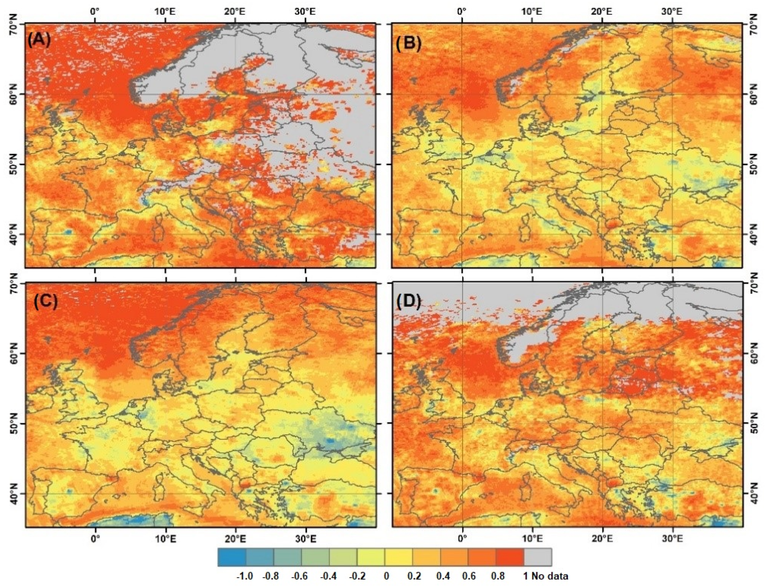
Figure 4 presents the spatial distribution of the emission correction factor for selected months in individual seasons. It was not possible to calculate the indicator, over the entire domain, for the winter months because of high cloud coverage. Negative values of the ratio indicate that the baseline emission should be increased, and the positive values of the calculated ratio indicate that the baseline emissions should be reduced. It should be noted that the negative values of the tropospheric NO2 columns that are caused by using the DOMINO method [35] were not used in the calculations.
The correction factor calculated based on the NO2 tropospheric column was applied to NO
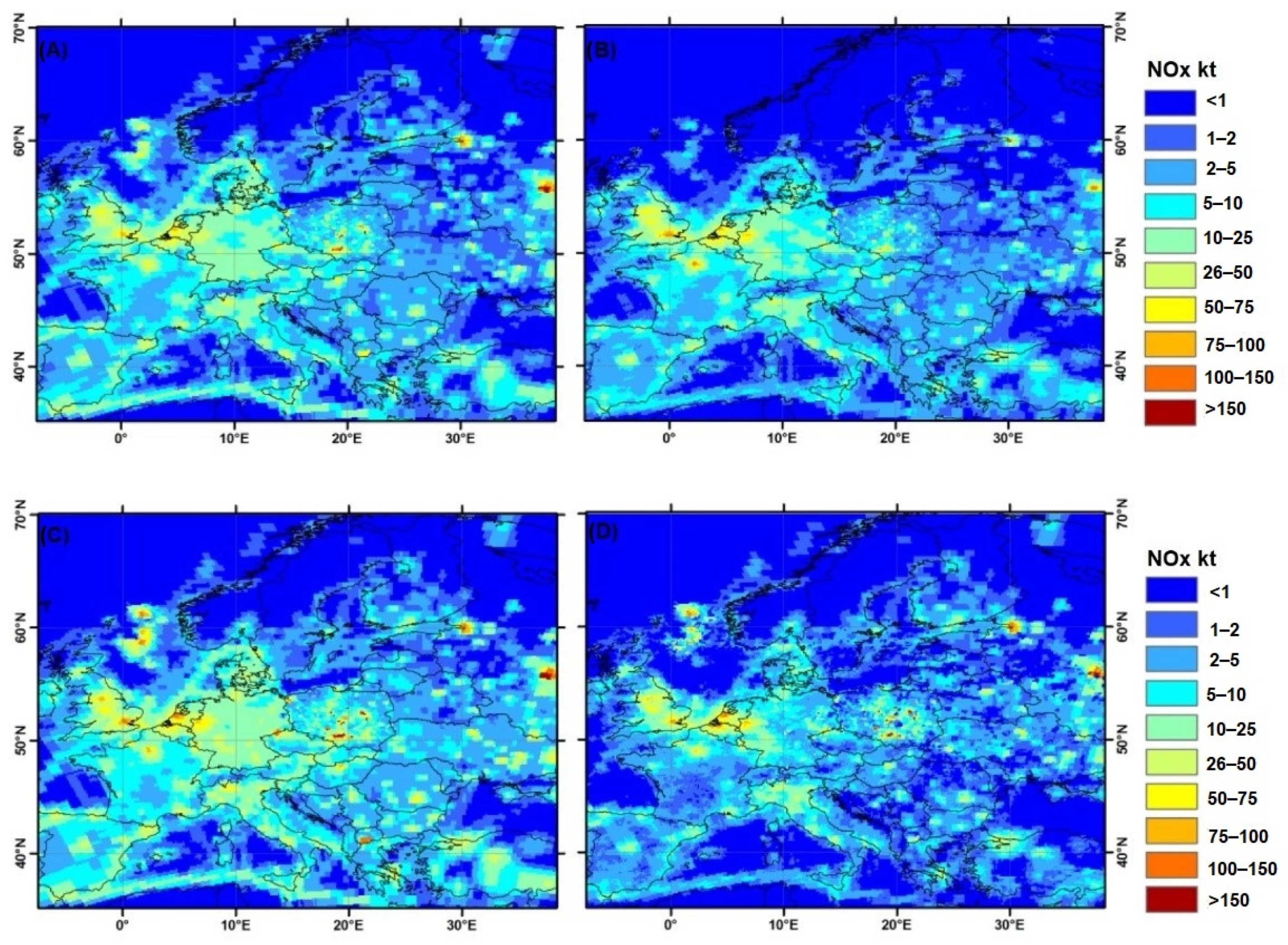
2 and NO emission fluxes. To process monthly emission fields, the annual emission budget from EMEP was monthly-distributed based on the temporal profile. Furthermore, the values of emission fluxes were modified by the correction factor, taking into account the magnitude of fluxes in each of the SNAP categories in a given grid square. Emission fluxes before and after modifications for July and December are shown in Figure 5.
After modification, more concentrated and higher fluxes of NOx emission were observed around agglomerations (average difference from 20 to 50 kt). Over the rural areas and the Mediterranean Sea, emissions were significantly lower. For the Mediterranean basin, the total emissions are reduced by almost half (from 51 to 28 Mt). In addition, some high values over inactive power plants have high decrees. For example, the region closest to the power plant in Bitola (Macedonia) registered a six-fold reduction (from 1000 to 150 kt) of the total emissions.

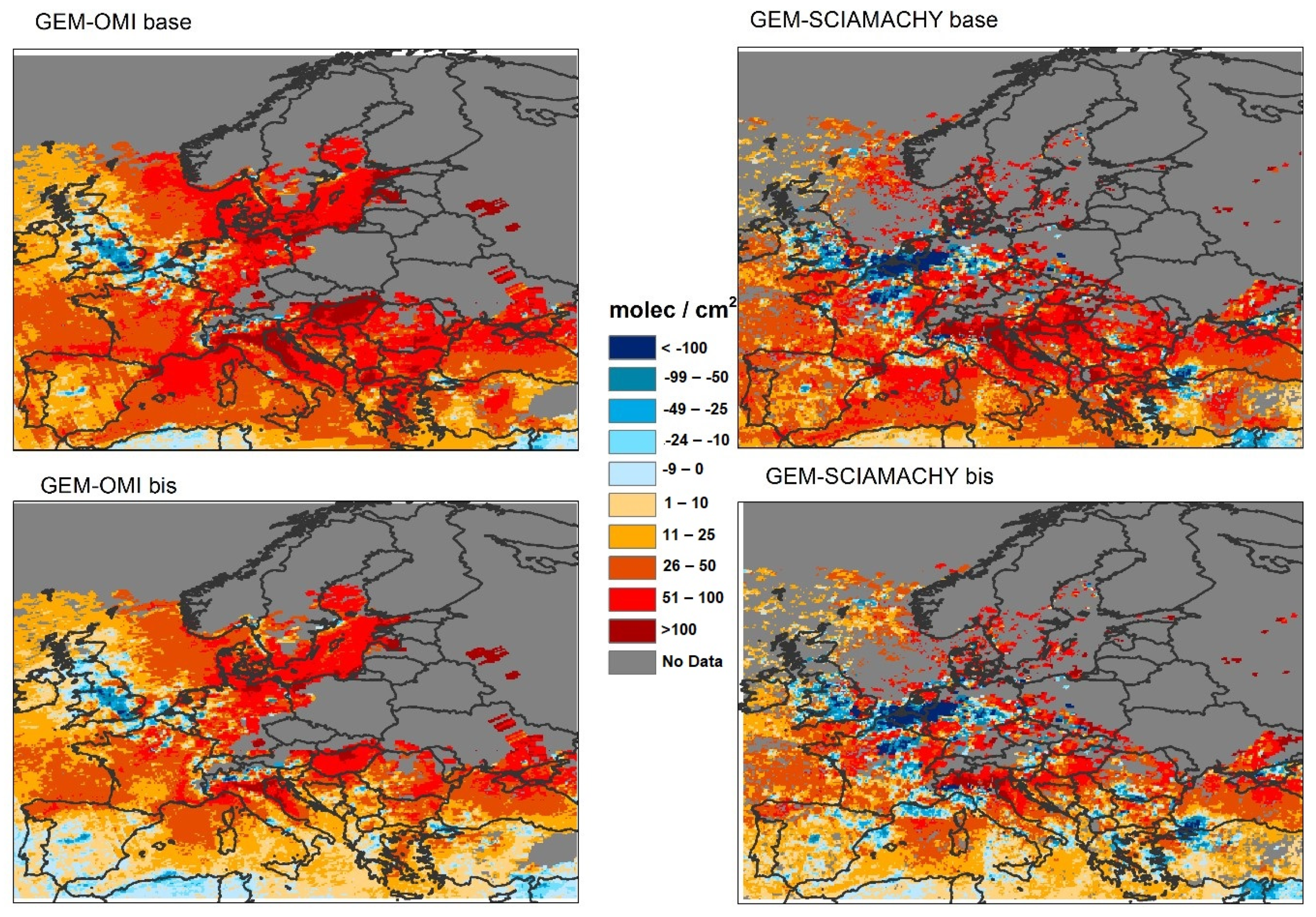
3.2. Modelled vs. Observed NO2 Column

Figure 6, Figure 7 and Figure 8 show a comparison between tropospheric columns observed by SCIAMACHY and OMI instruments for two simulations—with and without modification of NOx emissions for January, June, and August 2011, respectively.
In January, the spatial pattern is incomplete due to the cloud coverage, especially in northern and eastern Europe (Figure 8). Over the rest, a slight reduction of the positive bias can be found over the south of Europe: Spain, southern France, north Italy, and the Mediterranean Sea (from 10 to 25 × 1015 molec/cm2). In the case of negative bias, no significant improvement was found.
For June, the improvement is significant, especially in northern and central Europe. The overestimation over the North Sea, Poland, and the several agglomerations were reduced (from over 100 to 10–20 × 1015 molec/cm2), sometimes resulting in a slight underestimation (about 10–20 × 1015 molec/cm2). Similar to January, no significant changes in bias were detected for regions in western Europe characterised with underestimation.
For August, the general pattern of the differences between model and satellite observation was similar to those obtained for June.
Although in areas with significant underestimations, i.e., in the Benelux countries, an improvement of modelling results was not achieved. However, the underestimation was reduced from about 100 × 1015 molec/cm2 to approximately 40 × 1015 molec/cm2.

3.3. Chemical Regime

The insufficient increase of the modelled NO2 column value despite the significant increment of the emission flux may be related to the non-linearity between the concentration of NO2 and other photochemical species in the atmosphere and the ozone concentrations. An analysis of photochemical regimes was carried out to verify this hypothesis. In the scientific literature, the concept of chemical regimes refers mainly to near-surface ozone concentrations [36,37,38]. However, since NOx is a major ozone precursor, and the highest NOx concentrations are detected in the lowest 2 km (e.g., [8,39]), a regime-based concept was developed to analyse differences in chemical regimes in terms of the spatial pattern over Europe.
An indicator based on the ratio of O3 and NO2 was proposed. The partial columns of ozone (O3) and nitrogen dioxide (NO2) were calculated for the seven lowest model layers, i.e., up to about 1.400 m, representing the average height of the atmospheric boundary layer. The partial column ratio O3/NO2 was calculated for each month.
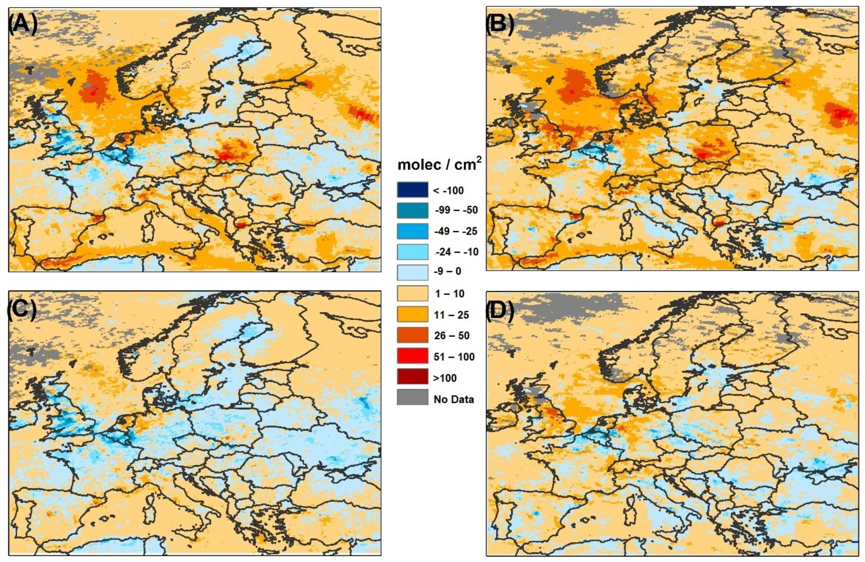
Figure 9 shows the average differences between the modelled tropospheric NO2 and the satellite observations averaged for two instruments for both simulations, as well as the O3/NO2 partial column ratio for the boundary layer for June 2011.
The photochemical regime index was the lowest over the region, with the strongest NO2 column underestimation for all months. This may indicate that in NOx-saturated regions, the differences between models and observations are not sensitive to the relatively small emissions perturbations and should be further analysed in the contacts of the photochemical cycle formulation.

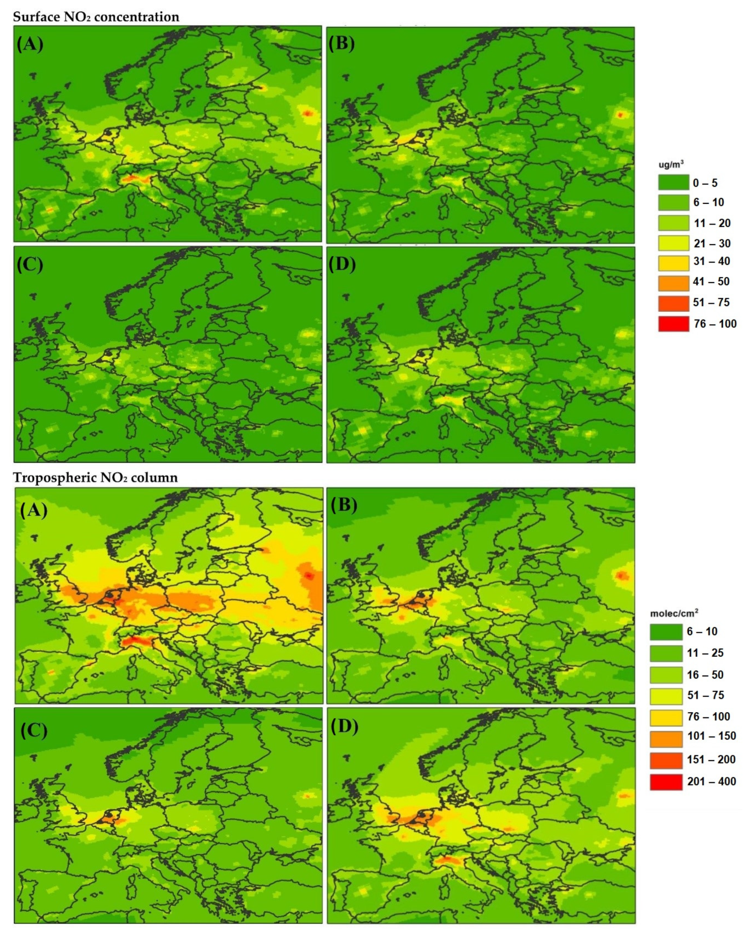
3.4. Modelled NO2—Tropospheric Column and Surface Concentrations

Although the tropospheric NO2 column does not fully reflect the near-surface emission sources, the regions for which the highest surface concentrations of NO2 were observed (over 40 µg/m3) coincide with the areas characterised by the highest values (over 100 × 1015 molec/cm2) of the tropospheric NO2 column calculated from model results. This relationship is particularly evident in the winter months. Surface NO2 concentration and NO2 column calculated from model results are high mostly, over large European agglomerations (e.g., Moscow, Paris, Madrid) and the Benelux countries (Figure 10).
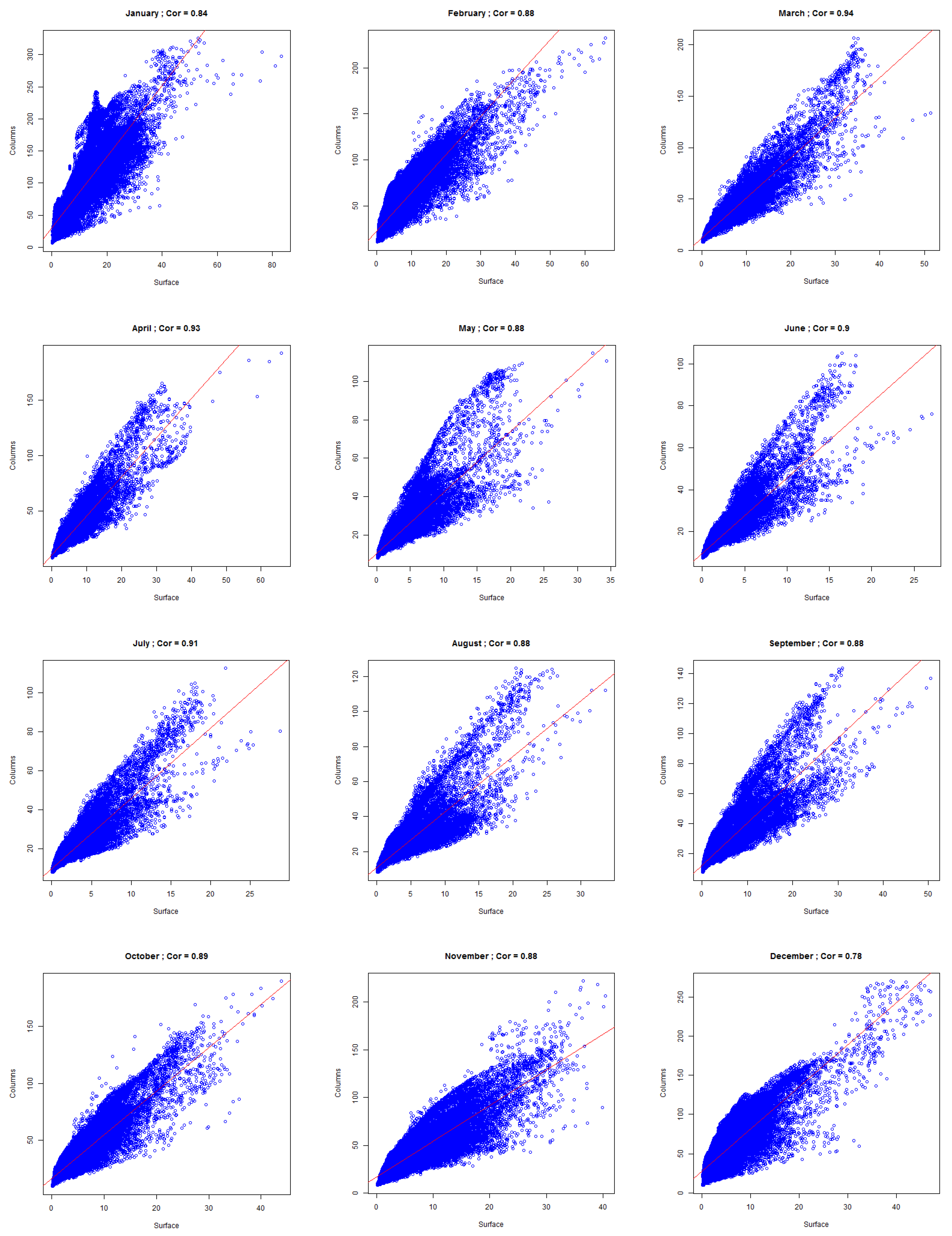
The relationship between the modelled surface NO2 concentrations and the value of the modelled tropospheric NO2 column is shown in Figure 11. A similar high correlation (>0.5) between OMI observations and ground-based in situ measurements was also recorded in important European Cities during 2005–2014 [40].
The observed dependency correlation coefficients between tropospheric NO2 columns and surface NO2 concentrations were calculated for all months in 2011 (Table 3). A high correlation in the range of 0.74 to 0.94 was calculated.

4. Discussion

High values of anthropogenic NOx emissions (over 40 µg/m3) are mainly recorded in urbanised and highly industrialised areas. In Europe, the highest NOx emissions occur primarily in large cities, such as London, Paris, Moscow, St. Petersburg, Istanbul, and Madrid and high maritime traffic in the Mediterranean. Higher NOx emission flux values were observed on the border of three countries: Germany, the Netherlands, and Belgium. In Poland, the highest values occur in the Silesia, Łódź, and Warsaw agglomerations.
Applied correction factors lead to an overall reduction of the emission budget over Europe. Table 4 summarises the monthly total emission fluxes calculated for the whole domain. Table 5 presents the total emission fluxes in selected countries as an annual total calculated from monthly values. Generally, modified emission fluxes are lower than the base case (Table 4). Reduction varies from 18% to 41%. The smallest reduction was calculated for April (1.06 × 10³ kt) and the highest was calculated for December (2.74 × 10³ kt). However, based on the comparison for individual countries, for Belgium, the emission flux of NOx increased after correction (0.01 × 10³ kt), and for the Netherlands, changes are relatively small (Table 5). A significant reduction of NOx emission budget followed by the improvement of the results indicates that there might be a systemic problem with the reporting of NOx emissions as the equivalent of NO2.
The correlation coefficients between NO2 columns derived from satellite observations (OMI and SCIAMACHY) and modelled by GEM-AQ for the base and modified emission scenarios were calculated to check if adjusted emissions improved the model performance. The correlation coefficient for columns from both spectrometers was enhanced by more than 0.1, and the extreme values were significantly reduced for the modified emission scenario.
The calculated correlations coefficients between the GEM-AQ base scenario and OMI-derived NO2 tropospheric columns were higher than for SCIAMACHY for all months except for July and August 2011. The lower correlation may be because there were more data from OMI than SCIAMACHY for the algorithm training period 2008–2010. The correlation coefficient for SCIAMACHY was higher for the months when cloud cover over Europe was relatively low.
It can be seen that with the modified emissions, the average monthly NO2 tropospheric column is better correlated with satellite data from SCIAMACHY and OMI (Table 6) for all months. For the summer months (June, July, August, and October), when a much larger number of observations were available to calculate the emission correction factors, the improvement of the correlation coefficient was ≈0.1. Significant improvement of the correlation coefficient was obtained for June and July (from 0.71 to 0.85) for SCIAMACHY.
The spatial distribution of the NO2 tropospheric column calculated by the GEM-AQ model for the modified emission scenario shows a significant improvement compared to the observed patterns. The improvement of correlation over the entire area is approximately >0.1 for the summer months (Table 6). In addition, for Benelux and Silesia practically for all months, an improvement of correlation (from 0.01 to 1.14) for 2011 was achieved (Table 7 and Table 8). A definite improvement of model results for the scenario with modified emissions was achieved over regions where emission fluxes were significantly reduced (North Sea, Mediterranean Sea, Silesia, Moscow, St. Petersburg). Systematic overestimations were reduced from 50–100·1015 to 10·1015 molec/cm2.
Although for Benelux, the correlation coefficient was generally higher than for Silesia (appropriately 0.42–0.93 and −0.5–0.83), and in most cases, correlation improved in the scenario with modified emissions, the negative bias change was relatively small. Qualitative analysis of the proposed indicator showed that the areas with a low O3/NO2 column ratio (below 10) coincide with regions characterised with the highest underestimation of the modelled NO2 column compared to satellite observations.
The high spatial agreement of NO2 tropospheric columns and surface concentrations suggests that modification of the anthropogenic emission fluxes may improve the distribution of NO2 columns and surface concentrations as calculated by the GEM-AQ model.
For 2011, we compare concentrations of NO2 with the model results for two scenarios (Base—with base emissions) and Bis (with modified emissions, using correction factors based on satellite data) for 14 stations (11 background rural, 2 background suburban, and 1 city station) in Poland. Statistical measures are given in Table 9. The analysis of the mean error shows that at most stations, on a yearly basis, there is a slight overestimation of the modelled NO2 concentrations. The mean square error for all stations is approximately ≈10 μg/m3.
For most stations, a relatively high correlation coefficient was obtained in the range of 0.60–0.75, which shows that the long- and short-term variability for the modelled concentrations is correctly reproduced. The station with a weak correlation in relation to the daily average values is Wrocław Bartnicza, where the variability of NO2 concentrations is controlled by the emission cycle, the phase of which was not correctly provided in the emissions inventory. Simulations with modified emissions gave slightly higher mean concentrations for all stations (change from 77.2 to 82.9 µg/m3). The mean RMSE for all stations was almost three times lower for the Bis scenario (change from 2.8 to 1.0 µg/m3).

5. Conclusions

A method for correcting nitrogen oxides anthropogenic emission fluxes was presented. The proposed emission correction method was developed using NO2 column observations from two spectrometers: OMI (on board the AURA satellite) and SCIAMACHY (on board the ENVISAT satellite) and results from a chemical weather model GEM-AQ.
The presented study verified whether using emissions correction factors calculated based on systematic differences between model results and satellite observations for the reference period would improve the distribution of the modelled NO2 columns and surface NO2 concentrations in the independent simulation. Emission correction factors were developed from model results and satellite observations over the period 2008–2010. Verification of the prosed emission corrections factors was carried out using an independent set of NO2 column observation and model simulations for 2011.
It was found that the modelled NO2 tropospheric column is strongly correlated with surface NO2 concentrations over the urban and polluted areas. The regions with the highest NO2 column and the highest surface concentration coincide. It confirms the hypothesis that both fields are mostly dependent on anthropogenic emissions, and the developed correction factors may improve the distribution of NO2 columns and surface concentrations. The developed method allows for modification of the emissions fluxes in areas where there were systematic differences between satellite observations and modelling results.
Application of the developed method could significantly improve model results in areas where the NO2 column was overestimated, e.g., inactive power plants, the Mediterranean Sea, and the North Sea.
There is a need to develop emission correction factors for parts of the modelling domain where the NO2 column was underestimated, e.g., Ukraine, Northern France, and England. Significant improvement after modification on NO2 emissions fluxes was not achieved. The expanded factors might take into account NOx-O3-VOC loss and production regimes.
Further development of emission correction factors and inverse modelling using satellite observations remains a very important area of research to refine estimates of anthropogenic emission fluxes. It is anticipated that future space observations and missions such as Sentinel 5p, 5, and 4 will provide additional information to support national policies in areas of air quality management and control.

Author Contributions

Conceptualization: K.S. and J.S.; methodology: J.W.K.; formal analysis: K.S., J.S. and J.W.K.; investigation: K.S.; writing—original draft preparation: K.S.; writing—review and editing: J.S. and J.W.K. All authors have read and agreed to the published version of the manuscript.

Funding

This research was funded by the National Science Centre granted number 2011/01/N/ST10/04725.

Institutional Review Board Statement

Not applicable.

Informed Consent Statement

Not applicable.

Data Availability Statement

Not applicable.

Conflicts of Interest

The authors declare no conflict of interest.

References

  1. Latza, U.; Gerdes, S.; Baur, X. Effects of nitrogen dioxide on human health: Systematic review of experimental and epidemiological studies conducted between 2002 and 2006. Int. J. Hyg. Environ. Health 2009, 212, 271–287. [Google Scholar] [CrossRef]
  2. Boningari, T.; Smirniotis, P.G. Impact of nitrogen oxides on the environment and human health: Mn-based materials for the NOx abatement. Curr. Opin. Chem. Eng. 2016, 13, 133–141. [Google Scholar]
  3. WHO. Health Aspects of Air Pollution with Particulate Matter, Ozone and Nitrogen Dioxide: Report on a WHO Working Group, Bonn, Germany, 13–15 January 2003; WHO Regional Office for Europe: Copenhagen, Denmark, 2003; p. 98. [Google Scholar]
  4. Lodgejr, J. Air quality guidelines. Global update 2005. Particulate matter, ozone, nitrogen dioxide and sulfur dioxide. Environ. Sci. Pollut. Res. 1996, 3, 23. [Google Scholar]
  5. EMEP/EAA. EMEP/EEA Air Pollutant Emission Inventory Guidebook 2016; Chapter 3. B Manure Management; The European Environment Agency: Copenhagen, Denmark, 2016; p. 62. [Google Scholar]
  6. Henriksen, J.F.; Bartonova, A.; Arnesen, K.; Rode, A. Convention on Long-Range Transboundary Air Pollution; Norsk Inst. for Luftforskning: Stockhol, Sweden, 1992. [Google Scholar]
  7. Tørseth, K.; Aas, W.; Breivik, K.; Fjæraa, A.M.; Fiebig, M.; Hjellbrekke, A.G.; Myhre, C.L.; Solberg, S.; Yttri, K.E. Introduction to the European Monitoring and Evaluation Programme (EMEP) and observed atmospheric composition change during 1972–2009. Atmos. Chem. Phys. Discuss. 2012, 12, 5447–5481. [Google Scholar] [CrossRef] [Green Version]
  8. Liang, J.; Horowitz, L.W.; Jacob, D.J.; Wang, Y.; Fiore, A.M.; Logan, J.A.; Gardner, G.M.; Munger, J.W. Seasonal budgets of reactive nitrogen species and ozone over the United States, and export fluxes to the global atmosphere. J. Geophys. Res. Atmos. 1998, 103, 13435–13450. [Google Scholar] [CrossRef]
  9. Martin, R.; Parrish, D.D.; Ryerson, T.B.; Nicks, D.K.; Chance, K.; Kurosu, T.P.; Jacob, D.J.; Sturges, E.D.; Fried, A.; Wert, B.P. Evaluation of GOME satellite measurements of tropospheric NO2 and HCHO using regional data from aircraft campaigns in the southeastern United States. J. Geophys. Res. Space Phys. 2004, 109, 1–11. [Google Scholar] [CrossRef]
  10. Ludwig, C.B.; Griggs, M.; Malkmus, W.; Bartle, E.J.R. Air Pollution Measurements from Satellites. 1973. Available online: https://www.osapublishing.org/ao/abstract.cfm?uri=ao-13-6-1494 (accessed on 3 November 2021).
  11. Zyrichidou, I.; Koukouli, M.E.; Balis, D.S.; Katragkou, E.; Melas, D.; Poupkou, A.; Kioutsioukis, I.; Van Der A, R.; Boersma, K.; Van Roozendael, M.; et al. Satellite observations and model simulations of tropospheric NO2 columns over south-eastern Europe. Atmos. Chem. Phys. Discuss. 2009, 9, 6119–6134. [Google Scholar] [CrossRef] [Green Version]
  12. Pay, M.T.; Jiménez-Guerrero, P.; Baldasano, J.M. Assessing sensitivity regimes of secondary inorganic aerosol formation in Europe with the CALIOPE-EU modeling system. Atmos. Environ. 2012, 51, 146–164. [Google Scholar] [CrossRef] [Green Version]
  13. Huijnen, V.; Eskes, H.J.; Poupkou, A.; Elbern, H.; Boersma, K.F.; Foret, G.; Sofiev, M.; Valdebenito, A.; Flemming, J.; Stein, O.; et al. Comparison of OMI NO2 tropospheric columns with an ensemble of global and European regional air quality models. Atmos. Chem. Phys. Discuss. 2010, 10, 3273–3296. [Google Scholar] [CrossRef] [Green Version]
  14. Kim, S.W.; Heckel, A.; Frost, G.J.; Richter, A.; Gleason, J.; Burrows, J.P.; McKeen, S.; Hsie, E.Y.; Granier, C.; Trainer, M. NO2 columns in the western United States observed from space and simulated by a regional chemistry model and their implications for NOx emissions. J. Geophys. Res. Atmos. 2009, 114, 1–29. [Google Scholar] [CrossRef] [Green Version]
  15. Constantin, D.-E.; Voiculescu, M.; Georgescu, L. Satellite Observations of NO2Trend over Romania. Sci. World J. 2013, 2013, 1–10. [Google Scholar] [CrossRef]
  16. Konovalov, I.B.; Beekmann, M.; Richter, A.; Burrows, J.P. Inverse modelling of the spatial distribution of NOx emissions on a continental scale using satellite data. Atmos. Chem. Phys. Discuss. 2006, 6, 1747–1770. [Google Scholar] [CrossRef] [Green Version]
  17. Burrows, J.P.; Weber, M.; Buchwitz, M.; Rozanov, V.; Ladstätter-Weißenmayer, A.; Richter, A.; DeBeek, R.; Hoogen, R.; Bramstedt, K.; Eichmann, K.-U.; et al. The Global Ozone Monitoring Experiment (GOME): Mission Concept and First Scientific Results. J. Atmos. Sci. 1999, 56, 151–175. [Google Scholar] [CrossRef]
  18. Bovensmann, H.; Burrows, J.P.; Buchwitz, M.; Frerick, J.; Noël, S.; Rozanov, V.V.; Chance, K.; Goede, A.P.H. SCIAMACHY: Mission Objectives and Measurement Modes. J. Atmos. Sci. 1999, 56, 127–150. [Google Scholar] [CrossRef] [Green Version]
  19. Blond, N.; Boersma, K.F.; Eskes, H.J.; van der A, R.J.; Van Roozendael, M.; De Smedt, I.; Bergametti, G.; Vautard, R. Intercomparison of SCIAMACHY nitrogen dioxide observations, in situ measurements and air quality modeling results over Western Europe. J. Geophys. Res. 2007, 112, D10311. [Google Scholar]
  20. Miyazaki, K.; Eskes, H.J.; Sudo, K. Global NOx emission estimates derived from an assimilation of OMI tropospheric NO2 columns. Atmos. Chem. Phys. 2012, 12, 2263–2288. [Google Scholar] [CrossRef] [Green Version]
  21. Vinken, G.C.M.; Boersma, K.F.; Van Donkelaar, A.; Zhang, L. Constraints on ship NOx emissions in Europe using GEOS-Chem and OMI satellite NO2 observations. Atmos. Chem. Phys. 2014, 14, 1353–1369. [Google Scholar]
  22. Levelt, P.F.; Van den Oord, G.H.J.; Dobber, M.R.; Malkki, A.; Visser, H.; de Vries, J.; Stammes, P.; Lundell, J.O.V.; Saari, H. The Ozone Monitoring Instrument. IEEE Trans. Geosci. Remote Sens. 2006, 44, 1093–1101. [Google Scholar] [CrossRef]
  23. Kawka, M.; Struzewska, J.; Kaminski, J. Spatial and Temporal Variation of NO2 Vertical Column Densities (VCDs) over Poland: Comparison of the Sentinel-5P TROPOMI Observations and the GEM-AQ Model Simulations. Atmosphere 2021, 12, 896. [Google Scholar] [CrossRef]
  24. Tong, D.Q.; Lamsal, L.; Pan, L.; Ding, C.; Kim, H.; Lee, P.; Chai, T.; Pickering, K.E.; Stajner, I. Long-term NOx trends over large cities in the United States during the great recession: Comparison of satellite retrievals, ground observations, and emission inventories. Atmos. Environ. 2015, 107, 70–84. [Google Scholar] [CrossRef]
  25. Szymankiewicz, K.; Kaminski, J.W.; Struzewska, J. Interannual variability of tropospheric NO2 column over central Europe—Observations from SCIAMACHY and GEM-AQ model simulations. Acta Geophys. 2014, 62, 915–929. [Google Scholar] [CrossRef]
  26. Kaminski, J.W.; Neary, L.; Struzewska, J.; McConnell, J.C.; Lupu, A.; Jarosz, J.; Toyota, K.; Gong, S.L.; Côté, J.; Liu, X.; et al. GEM-AQ, an on-line global multiscale chemical weather modelling system: Model description and evaluation of gas phase chemistry processes. Atmos. Chem. Phys. Discuss. 2008, 8, 3255–3281. [Google Scholar] [CrossRef] [Green Version]
  27. Informative Inventory Report. 2021. Submission under the UNECE CLRTAP and NEC Directive. Available online: https://www.ceip.at/status-of-reporting-and-review-results/2021-submission/#E (accessed on 3 November 2021).
  28. Cuvelier, C.; Thunis, P.; Vautard, R.; Amann, M.; Bessagnet, B.; Bedogni, M.; Berkowicz, R.; Brandt, J.; Brocheton, F.; Builtjes, P.; et al. CityDelta: A model intercomparison study to explore the impact of emission reductions in European cities in 2010. Atmos. Environ. 2007, 41, 189–207. [Google Scholar] [CrossRef]
  29. Colette, A.; Andersson, C.; Manders, A.; Mar, K.; Mircea, M.; Pay, M.-T.; Raffort, V.; Tsyro, S.; Cuvelier, C.; Adani, M.; et al. EURODELTA-Trends, a multi-model experiment of air quality hindcast in Europe over 1990–2010. Geosci. Model Dev. 2017, 10, 3255–3276. [Google Scholar] [CrossRef] [Green Version]
  30. Rao, S.T.; Galmarini, S.; Puckett, K. Air Quality Model Evaluation International Initiative (AQMEII): Advancing the State of the Science in Regional Photochemical Modeling and Its Applications. Bull. Am. Meteorol. Soc. 2011, 92, 23–30. [Google Scholar] [CrossRef] [Green Version]
  31. Simpson, D.; Benedictow, A.; Berge, H.; Bergström, R.; Emberson, L.D.; Fagerli, H.; Flechard, C.R.; Hayman, G.D.; Gauss, M.; Jonson, J.E.; et al. The EMEP MSC-W chemical transport model—Technical description. Atmos. Chem. Phys. 2012, 12, 7825–7865. [Google Scholar] [CrossRef] [Green Version]
  32. Bieser, J.; Aulinger, A.; Matthias, V.; Quante, M.; van der Gon, H.D. Vertical emission profiles for Europe based on plume rise calculations. Environ. Pollut. 2011, 159, 2935–2946. [Google Scholar] [CrossRef] [Green Version]
  33. Struzewska, J.; Kaminski, J.W.; Durka, P.; Szymankiewicz, K. Operational Forecasting of Tropospheric Ozone Concentrations Using Modeling in 2015; Główny Inspektorat Ochrony Środowiska: Warsaw, Poland, 2015. [Google Scholar]
  34. Vidic, S. Frequency distributions of effective plume height. In Proceedings of the Frequency Distributions of Effective Plume Height, Zagreb, Croatia, 10 September 2002. [Google Scholar]
  35. Boersma, K.F.; Eskes, H.J.; Dirksen, R.J.; Van Der A, R.J.; Veefkind, J.P.; Stammes, P.; Huijnen, V.; Kleipool, Q.L.; Sneep, M.; Claas, J.; et al. An improved tropospheric NO2 column retrieval algorithm for the Ozone Monitoring Instrument. Atmos. Meas. Tech. 2011, 4, 1905–1928. [Google Scholar] [CrossRef] [Green Version]
  36. Beekmann, M.; Vautard, R. A modelling study of photochemical regimes over Europe: Robustness and variability. Atmos. Chem. Phys. Discuss. 2010, 10, 10067–10084. [Google Scholar] [CrossRef] [Green Version]
  37. Jiménez, P.; Baldasano, J.M. Ozone response to precursor controls in very complex terrains: Use of photochemical indicators to assess O3-NOx-VOC sensitivity in the northeastern Iberian Peninsula. J. Geophys. Res. D Atmos. 2004, 109, 1–20. [Google Scholar]
  38. Millard, F.; Toupance, G. Indicators Concept Applied to a European City: The Ile de France Area during ESQUIF Campaign. In Air Pollution Modelling and Simulation; Springer: Berlin/Heidelberg, Germany, 2002; pp. 54–58. [Google Scholar]
  39. Schaub, D.; Boersma, K.F.; Kaiser, J.W.; Weiss, A.K.; Folini, D.; Eskes, H.J.; Buchmann, B. Comparison of GOME tropospheric NO2 columns with NO2 profiles deduced from ground-based in situ measurements. Atmos. Chem. Phys. Discuss. 2006, 6, 3211–3229. [Google Scholar] [CrossRef] [Green Version]
  40. Paraschiv, S.; Constantin, D.E.; Paraschiv, S.L.; Voiculescu, M. OMI and ground-based in-situ tropospheric nitrogen dioxide observations over several important European cities during 2005–2014. Int. J. Environ. Res. Public Health 2017, 14, 1415. [Google Scholar] [CrossRef] [PubMed] [Green Version]
Figure 1. Emissions of nitrogen oxides NOx as NO2 for EU28 from EMEP. Yellow colours of bars represent the years of analysis in the presented work, and blue bars represent other years.
Atmosphere 12 01465 g001
Figure 2. Emissions of nitrogen oxides NOx as NO2 for EU28 (A) and Poland (B) divided into different SNAP97 sectors, based on the EMEP database for the period 2008–2010.
Atmosphere 12 01465 g002
Figure 3. Core grid with a uniform resolution of 0.125 deg (red line—numerical equator).
Atmosphere 12 01465 g003
Figure 4. Correction ratio values (F) for NOx emission based on satellite data and GEM–AQ model results. (A) February, (B) May, (C) August, and (D) November.
Atmosphere 12 01465 g004
Figure 5. Comparison of NOx emission fluxes in 2010 for July (upper panels) and December (lower panels) before (left panels) and after (right panels) modifications.
Atmosphere 12 01465 g005
Figure 6. Differences (1015 molec/cm2) in the tropospheric NO2 columns derived from GEM-AQ for the baseline emissions (upper row) and the modified emissions (bottom row) and satellite observations (OMI left, right SCIAMACHY) for January 2011.
Atmosphere 12 01465 g006
Figure 7. Differences (1015 molec/cm2) in the tropospheric NO2 columns derived from GEM-AQ for the baseline emissions (upper row) and the modified emissions (bottom row) and satellite observations (OMI left, right SCIAMACHY) for June 2011.
Atmosphere 12 01465 g007
Figure 8. Differences (1015 molec/cm2) in the tropospheric NO2 columns derived from GEM-AQ for the baseline emissions (upper row) and the modified emissions (bottom row) and satellite observations (OMI left, right SCIAMACHY) for August 2011.
Atmosphere 12 01465 g008
Figure 9. The difference between NO2 tropospheric columns derived from the model results and observations from satellite (OMI + SCIAMACHY) for the Base and Bis scenarios and ratio O3/NO2 column for June 2011.
Atmosphere 12 01465 g009
Figure 10. Surface NO2 concentration fields (top panel) and tropospheric NO2 column (bottom panel) for 2010 were calculated for a selected month by the GEM-AQ. (A) February, (B) April, (C) August, (D) October.
Atmosphere 12 01465 g010
Figure 11. Relation between NO2 tropospheric columns (Y axis) and surface concentrations NO2 (X axis) from the GEM-AQ model (single point represent one grid point).
Atmosphere 12 01465 g011
Table 1. Contribution of NOx emissions by individual SNAP category (Selected Nomenclature for sources of Air Pollution).
NoSNAP CategorySNAP DescriptionEU27PolandDenmarkNetherland
101Energy exploration and production18%33%19%13%
202Commercial, intuitional and households5%10%6%12%
303Energy in use8%9%4%11%
404 & 05Industrial processes3%2%0%0%
506Solvent and product use0%0%0%0%
607Road transport32%33%37%38%
708Non-road transport33%12%34%23%
809Waste0%0%0%0%
910Agriculture1%1%0%3%
Table 2. Surface air quality stations used in the analysis.
NoStation NameStation TypeLatitudeLongitude
1CzerniawaBackground rural16°56.52′ E50°17.82′ N
2Bory TucholskieBackground rural17°55.98′ E53°39.00′ N
3WiduchowaBackground rural14°23.82′ E53°10.32′ N
4KrzyżówkaBackground rural22° 04.14′ E54°09.00′ N
5Granica KPNBackground rural21°07.32′ E49°38.64′ N
6SzymbarkBackground rural15°16.02′ E52°13.32′ N
7Smolary BytnickieBackground rural19°33.84′ E51°20.82′ N
8ParzniewiceBackground rural16°25.32′ E51°59.64′ N
9GajewBackground rural19°13.98′ E52°13.98′ N
10Biały SłupBackground rural22°59.76′ E50°35.46′ N
11Belsk Background rural20°52.02′ E51°52.02′ N
12Wrocław BartniczaBackground suburban17°08.46′ E51°06.90′ N
13LegionowoBackground suburban 20°30.84′ E52°18.66′ N
14BiałystokUrban 23°20.82′ E53°13.32′ N
Table 3. Pearson correlation coefficients between tropospheric NO2 column and surface concentrations for 2011.
JanFebMarAprMayJunJulAugSeptOctNovDec
0.840.880.940.930.880.900.910.880.880.890.880.78
Table 4. Emission of NOx (103 kt) for Europe before and after modification.
JanFebMarAprMayJunJulAugSeptOctNovDec
Base6.736.546.305.865.445.235.235.235.375.846.336.70
Mod.4.673.944.404.803.963.723.903.964.093.903.793.96
Table 5. The monthly mean value of emission NOx (103 kt) before and after modification.
PolandFranceNetherlandBelgiumGermany
Base0.350.370.110.070.50
Mod.0.220.310.100.080.40
Table 6. Correlation coefficients between NO2 tropospheric column from satellite data and GEM-AQ base emission (BE) and modified emission (ME) scenarios for 2011 over the entire modelled domain.
All AreaMonth
JanFebMarAprMayJunJulAugSeptOctNovDec
OMI-GEM (BE)0.640.680.860.830.800.740.690.730.770.780.780.60
OMI-GEM (ME)0.680.740.920.890.880.850.780.820.880.870.830.65
SCIAMACHY-GEM (BE) 0.540.580.660.720.780.710.710.750.700.600.600.54
SCIAMACHY-GEM (ME) 0.610.580.690.820.850.850.850.850.830.700.660.53
Table 7. Correlation coefficients between NO2 tropospheric column from satellite data and GEM-AQ base emission (BE) and modified emission (ME) scenarios for 2011 for the Benelux part of the modelling domain.
All AreaMonth
JanFebMarAprMayJunJulAugSeptOctNovDec
OMI-GEM (BE)0.550.750.830.790.920.450.660.670.880.870.830.71
OMI-GEM (ME)0.580.730.930.870.890.650.700.710.890.890.860.74
SCIAMACHY-GEM (BE) 0.650.680.600.630.890.690.770.830.710.660.760.42
SCIAMACHY-GEM (ME) 0.690.680.760.750.870.820.770.860.740.730.700.47
Table 8. Correlation coefficients between NO2 tropospheric column from satellite data and GEM-AQ base emission (BE) and modified emission (ME) for 2011 for the Silesia part of the modelling domain.
All AreaMonth
JanFebMarAprMayJunJulAugSeptOctNovDec
OMI-GEM (BE)−0.50−0.10.710.580.730.160.530.510.820.610.570.00
OMI-GEM (ME)−0.50−0.10.710.610.770.240.550.600.780.540.670.20
SCIAMACHY-GEM (BE) 0.230.250.520.430.590.330.410.560.800.250.530.52
SCIAMACHY-GEM (ME) 0.220.240.580.410.620.410.430.700.830.330.620.45
Table 9. Statistical measures for two scenarios (Base—with base emissions) and Bis (with modified emissions, using correction factors based on satellite data) calculated for 2011.
StationMeanMRSECorrelation
BaseBisBaseBisBaseBis
Czerniawa75.6174.641.340.330.400.27
Bory Tucholskie176.83180.487.867.560.490.54
Widuchowa51.0952.351.09−1.090.610.53
Krzyżówka53.1445.77−1.33−1.120.620.55
Granica KPN101.28149.028.225.160.570.61
Szymbark49.1237.640.90−2.340.790.67
Smolary Bytnickie166.23204.095.634.840.700.79
Parzniewice72.5065.480.571.830.530.47
Gajew64.5352.924.773.690.770.69
Biały Słup48.6943.09−0.19−2.490.760.75
Belsk58.0566.813.200.910.600.56
Wrocław Bartnicza61.0374.314.721.490.130.22
Legionowo48.3264.322.33−2.570.530.64
Białystok54.3350.470.13−1.610.590.53
Publisher’s Note: MDPI stays neutral with regard to jurisdictional claims in published maps and institutional affiliations.

