
High-Resolution Modelling of Thermal Exposure during a Hot Spell: A Case Study Using PALM-4U in Prague, Czech Republic

 , , and
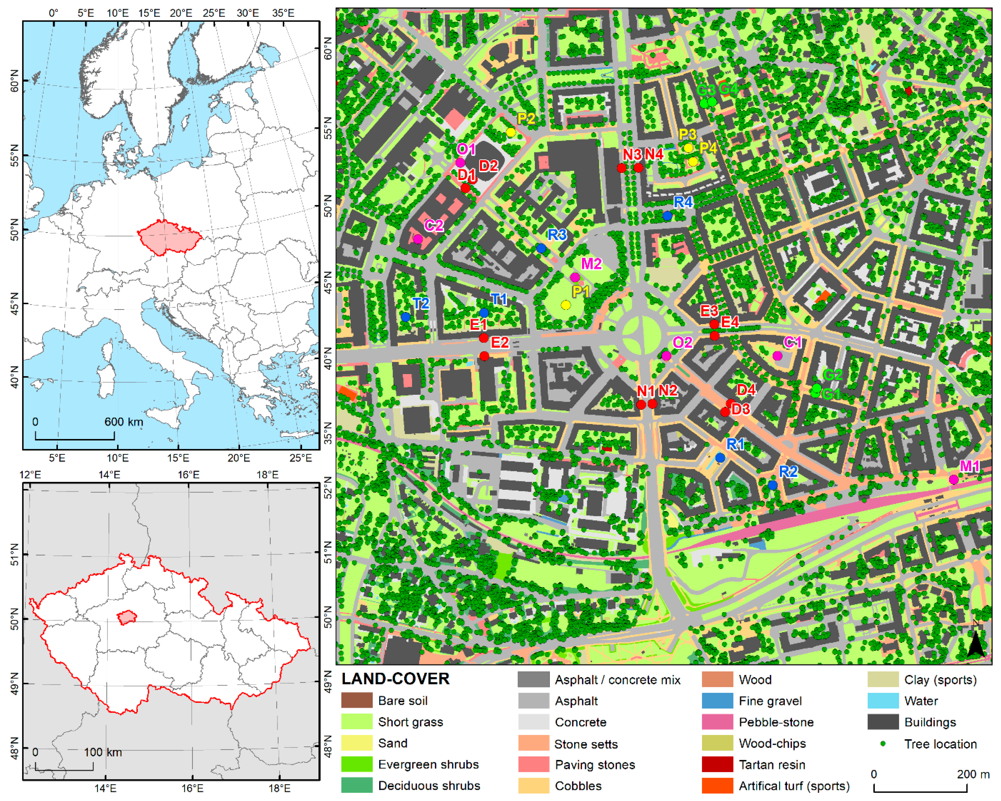
Abstract
:1. Introduction
2. Theoretical Background
2.1. Thermal Exposure in Urban Areas
2.2. Modelling Thermal Exposure in the Urban Environment
3. Study Area and Meteorological Conditions
3.1. Domain Description
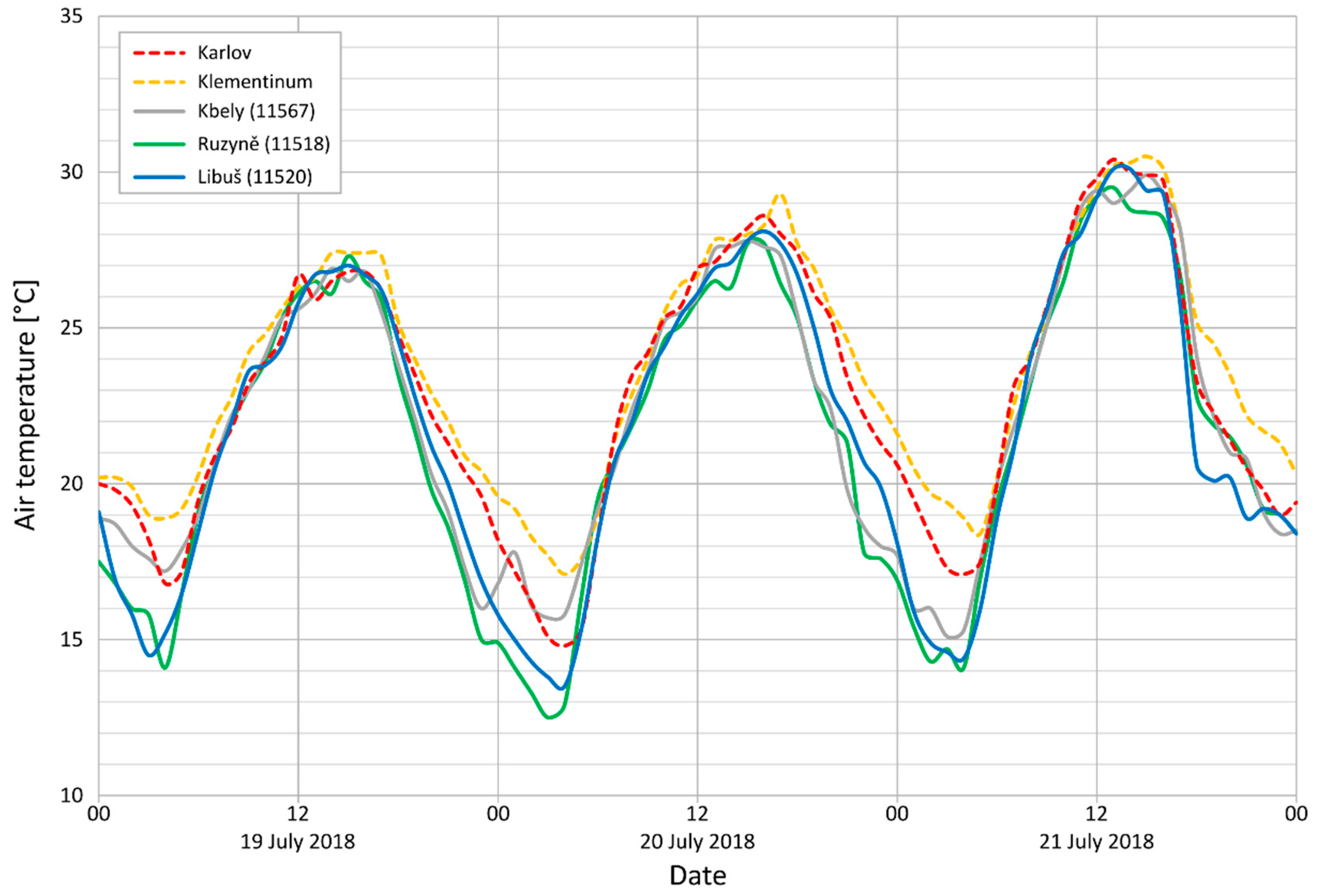
3.2. Meteorological Conditions
4. Data and Methods
4.1. GIS Data
4.2. PALM-4U Model Setup
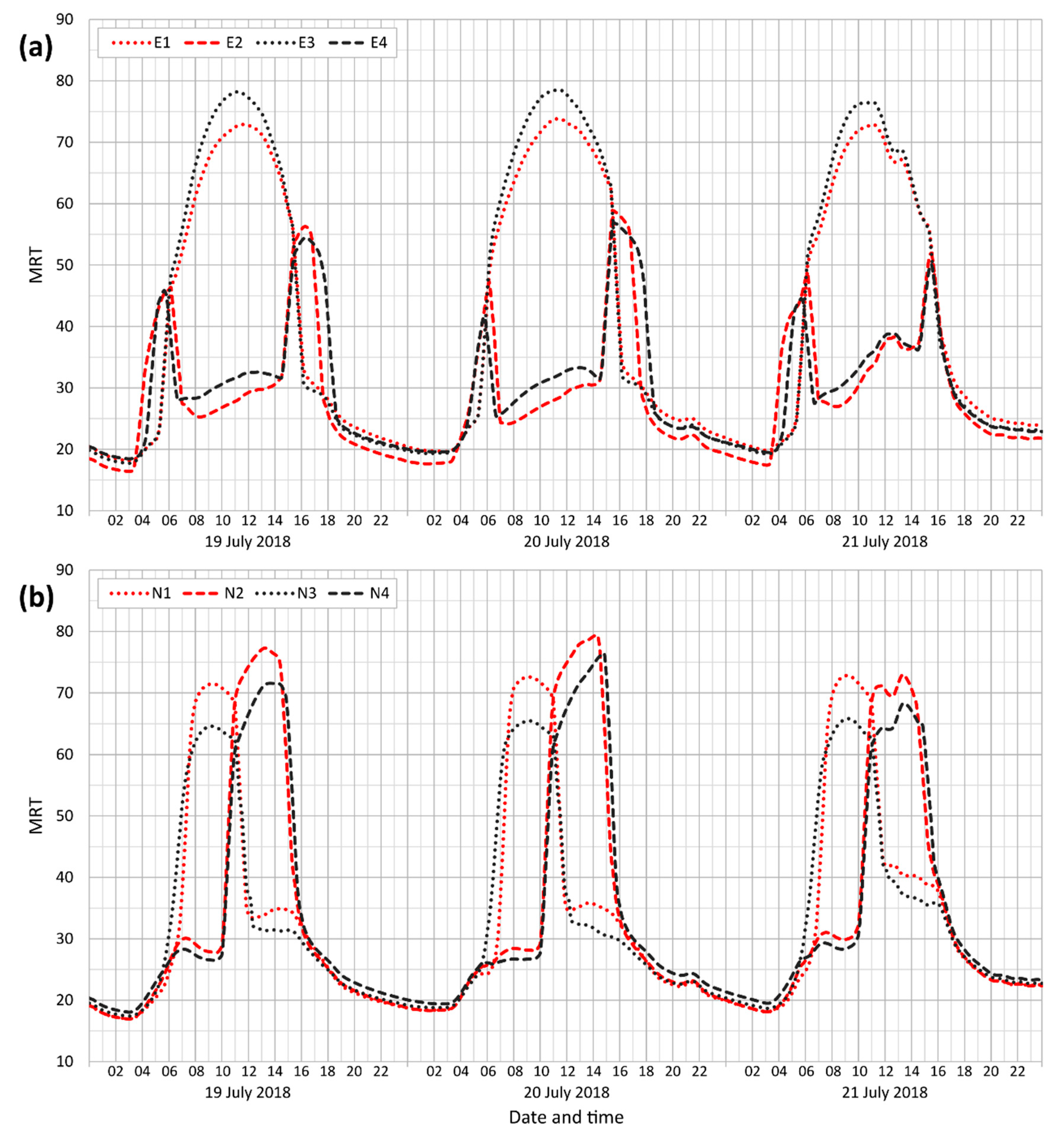
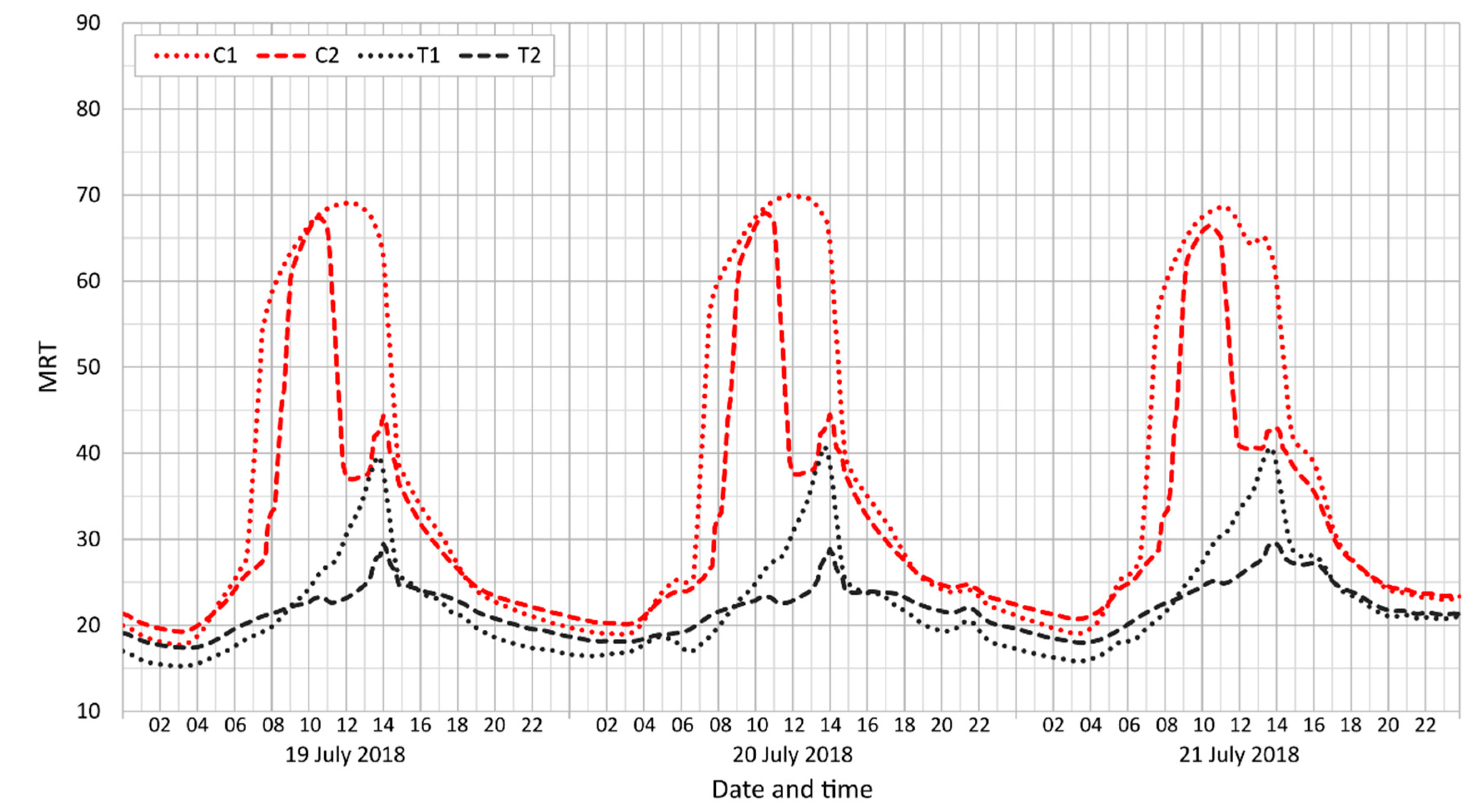
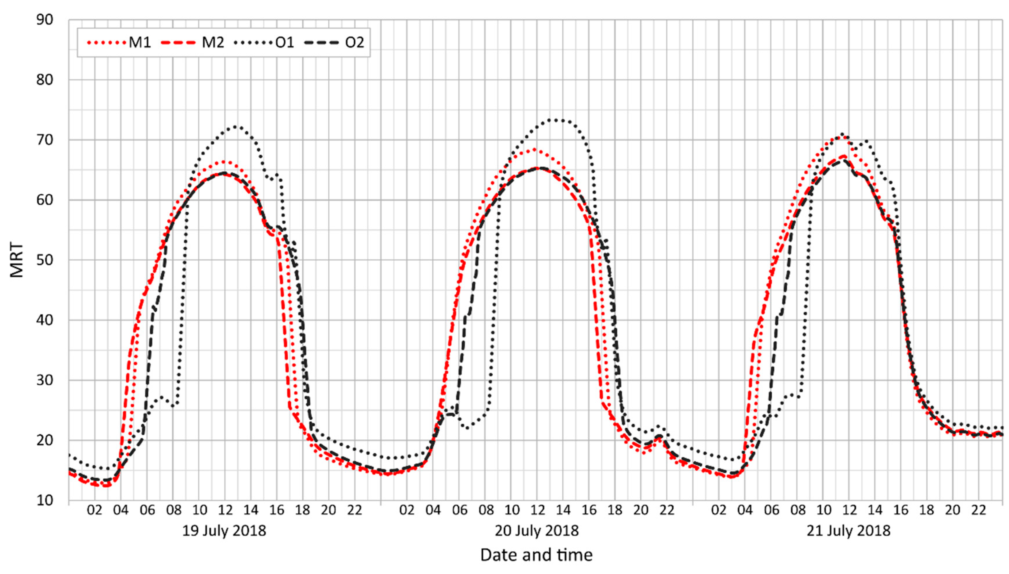
4.2.1. Mean Radiant Temperature Calculation
4.2.2. Universal Thermal Climate Index calculation
4.3. Model Validation
5. Results
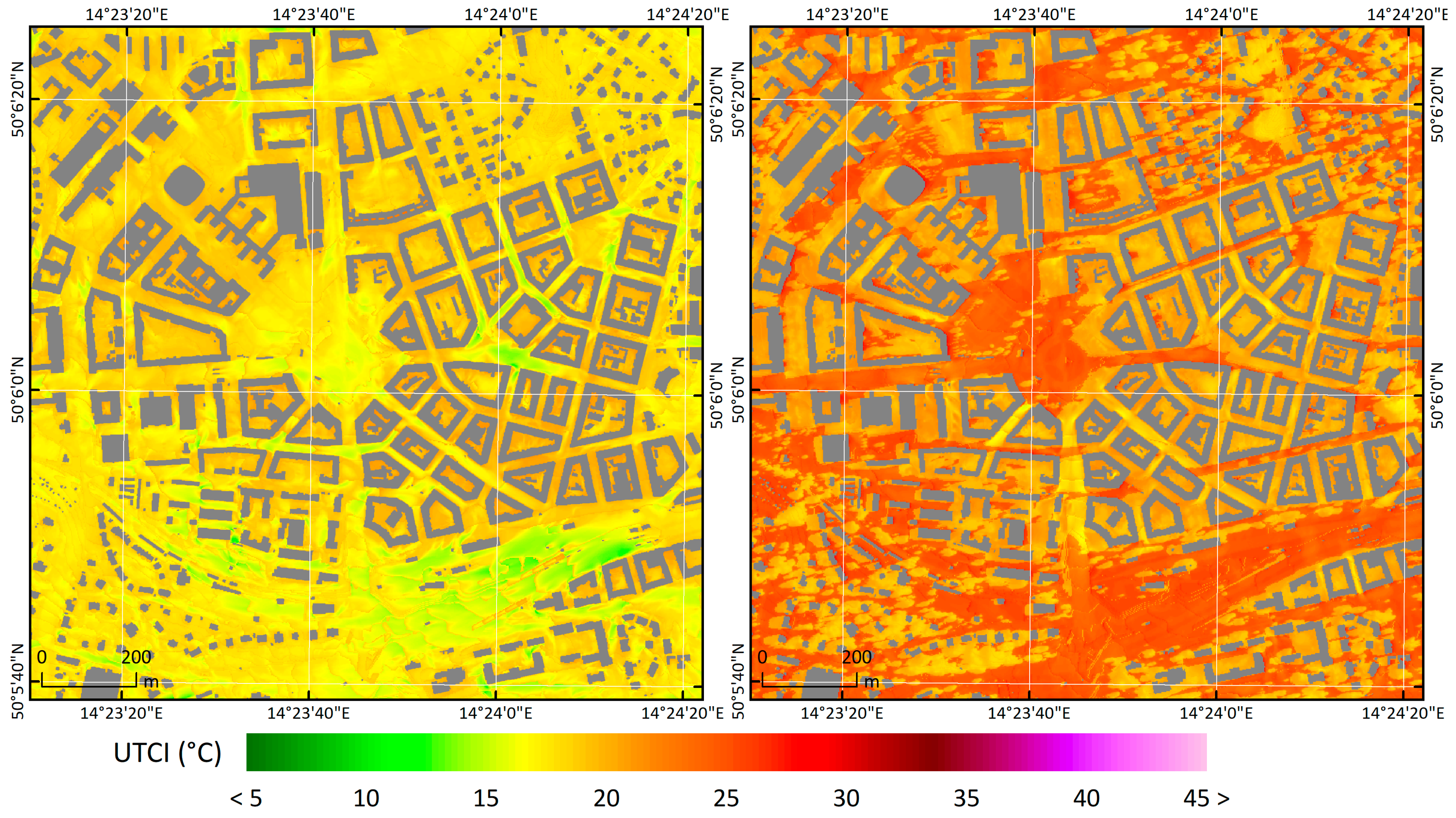
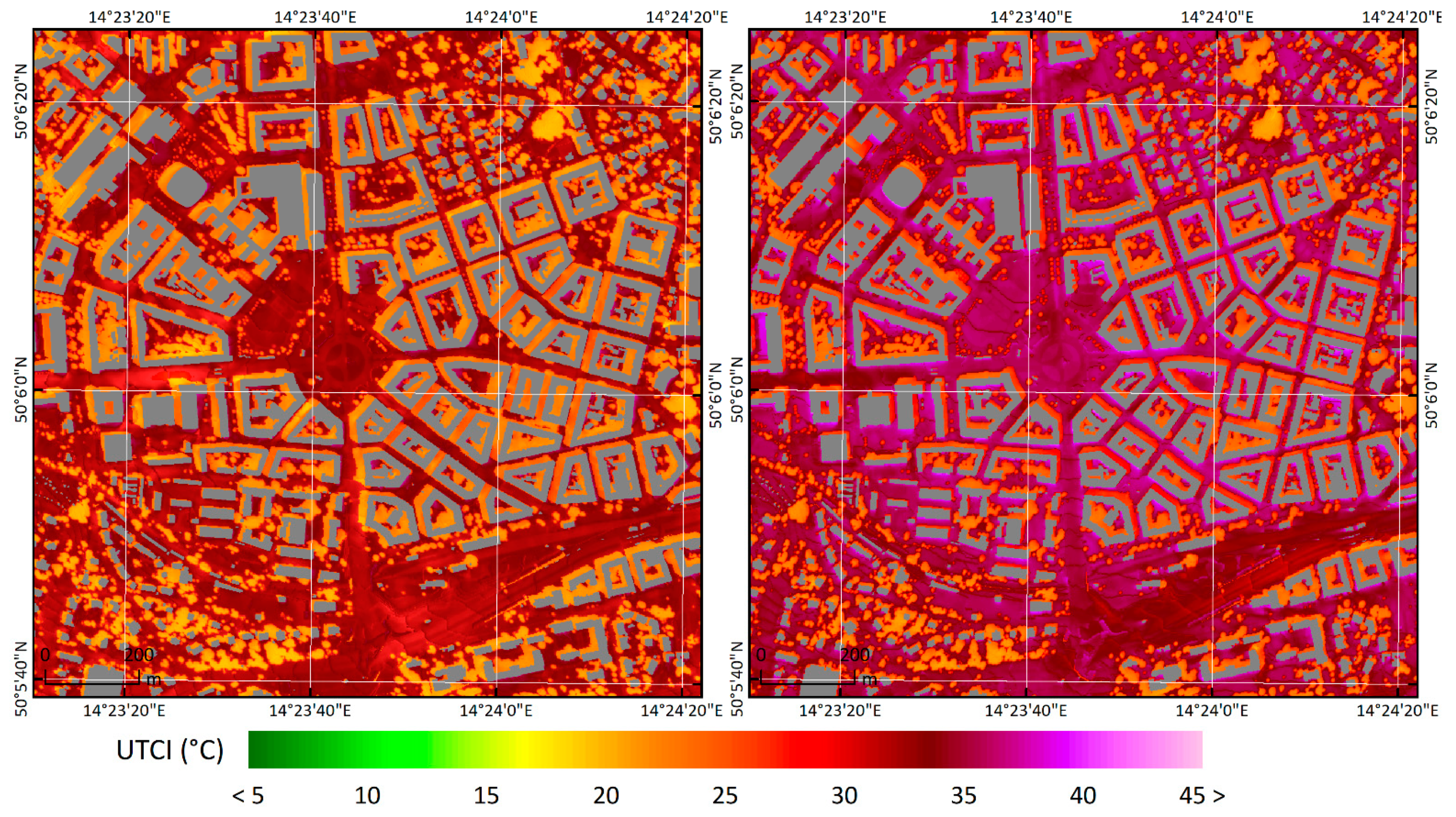
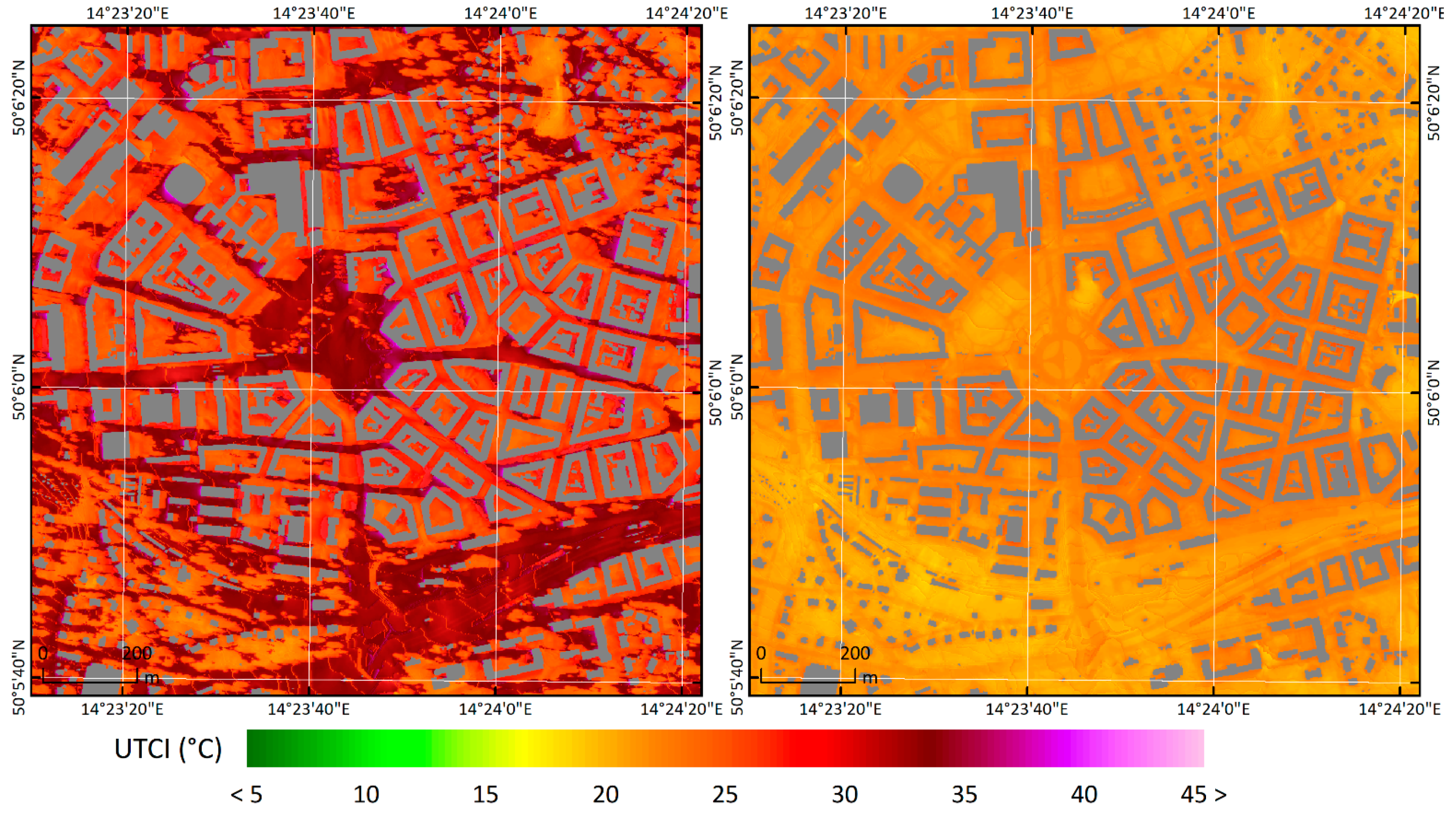
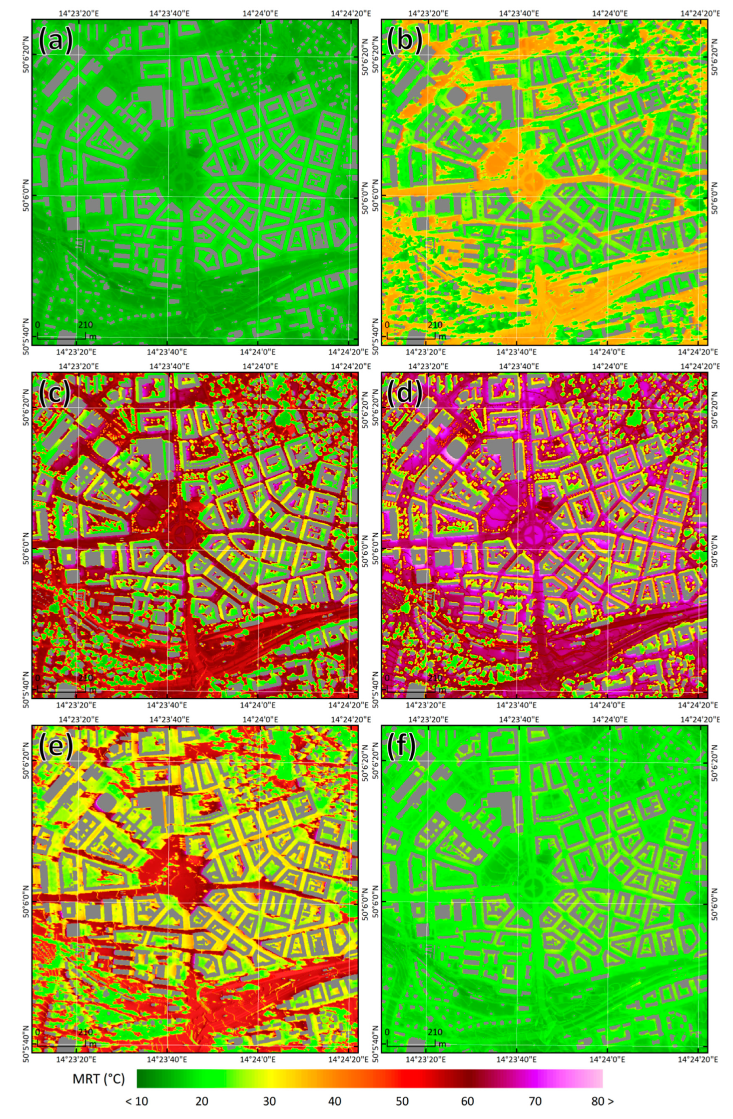
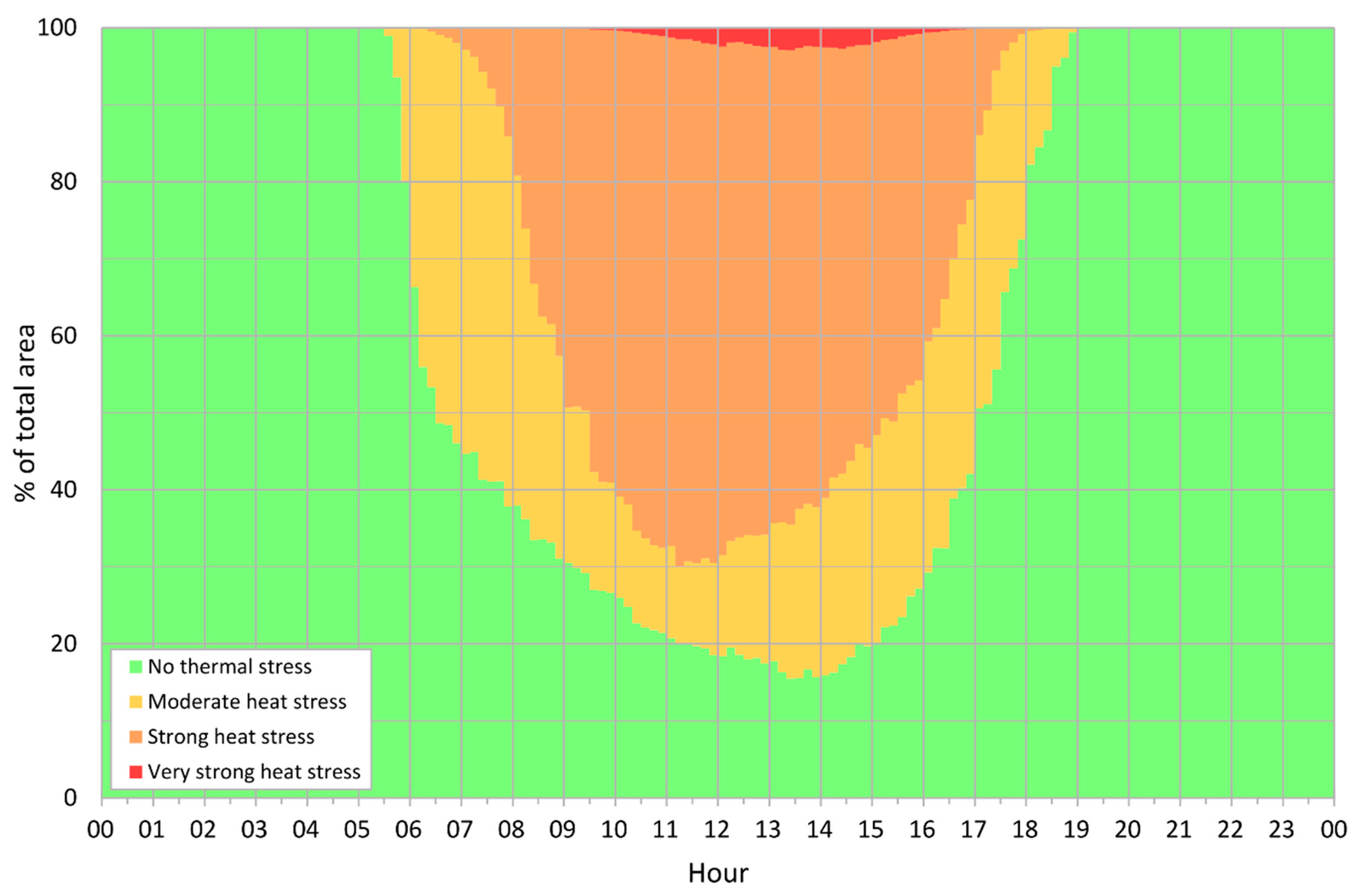
5.1. Spatiotemporal Pattern of Thermal Exposure in Urban Area
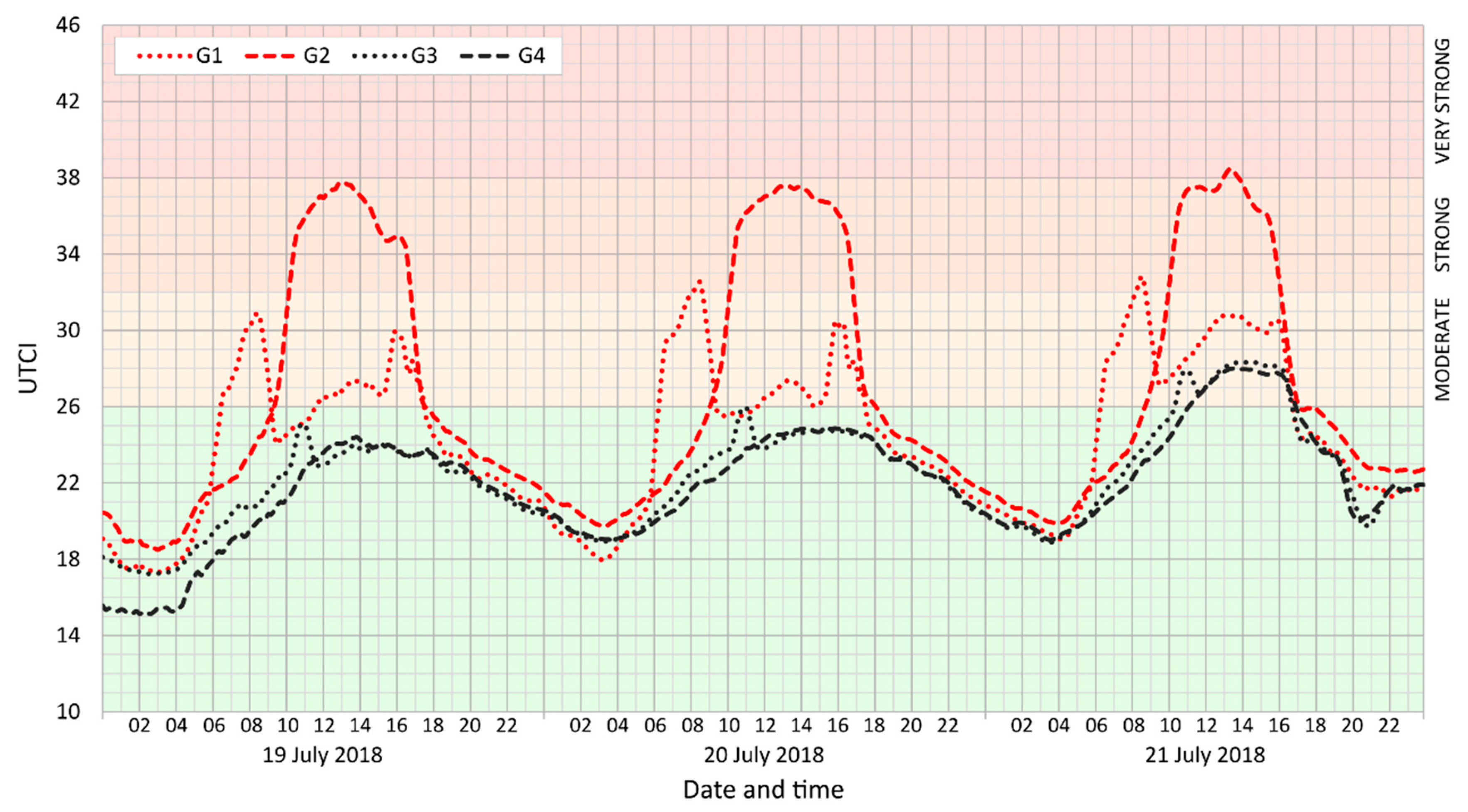
5.2. Daily Course of UTCI in an Urban Area
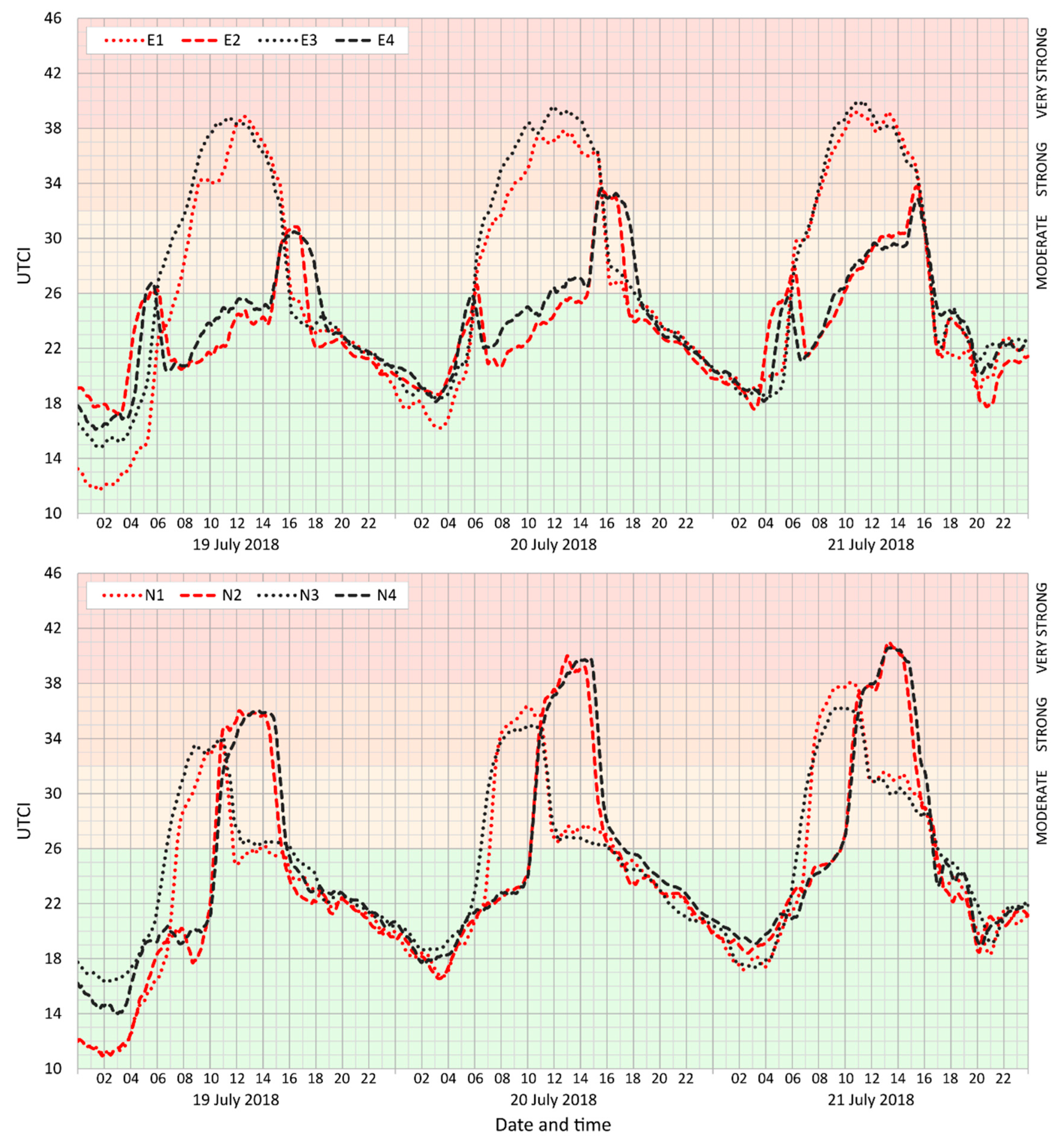
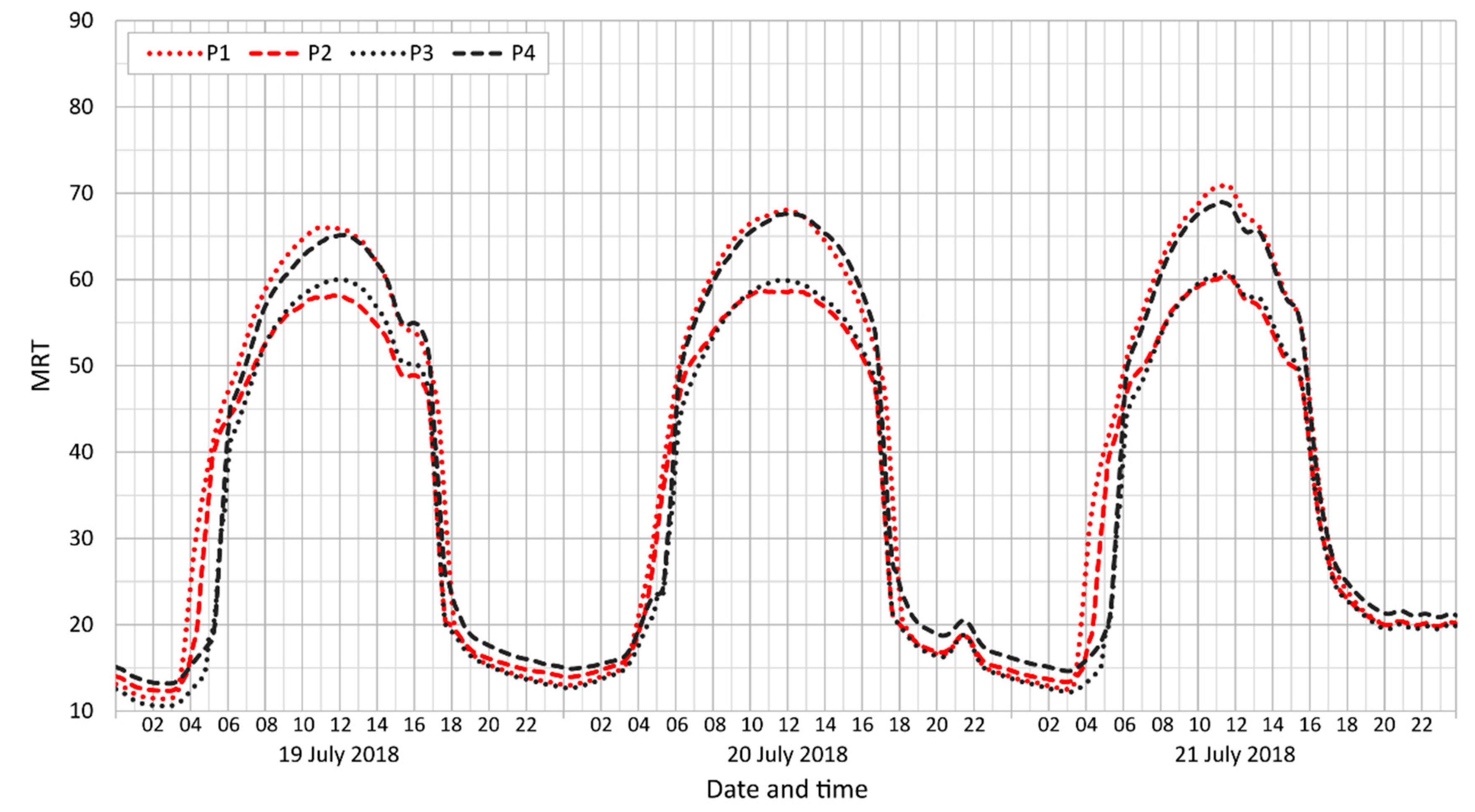
5.2.1. Streets (Canyons)
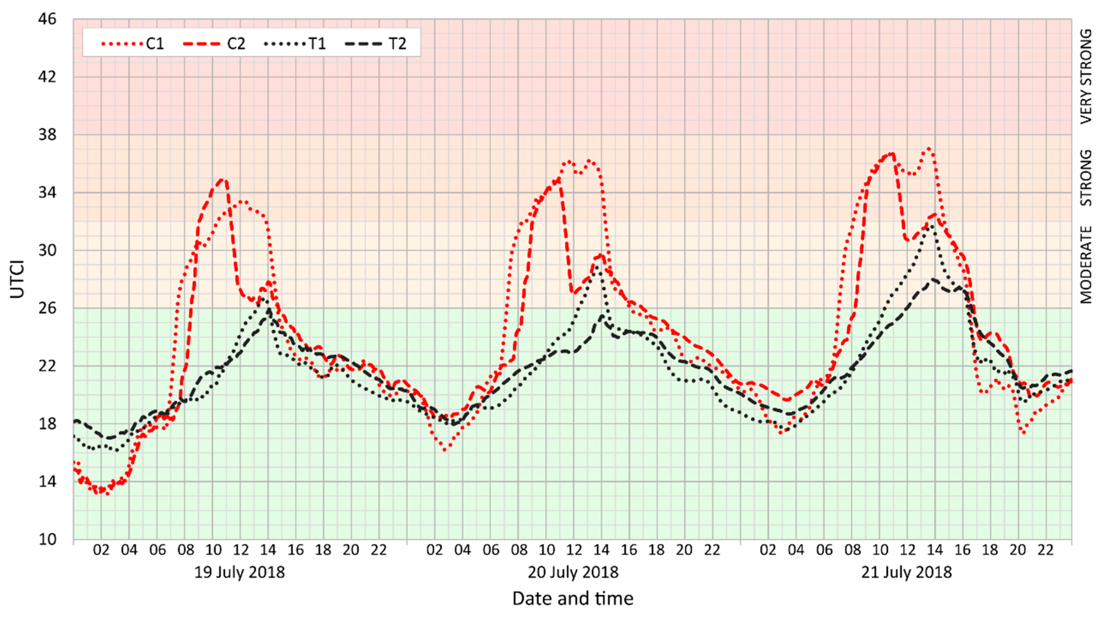
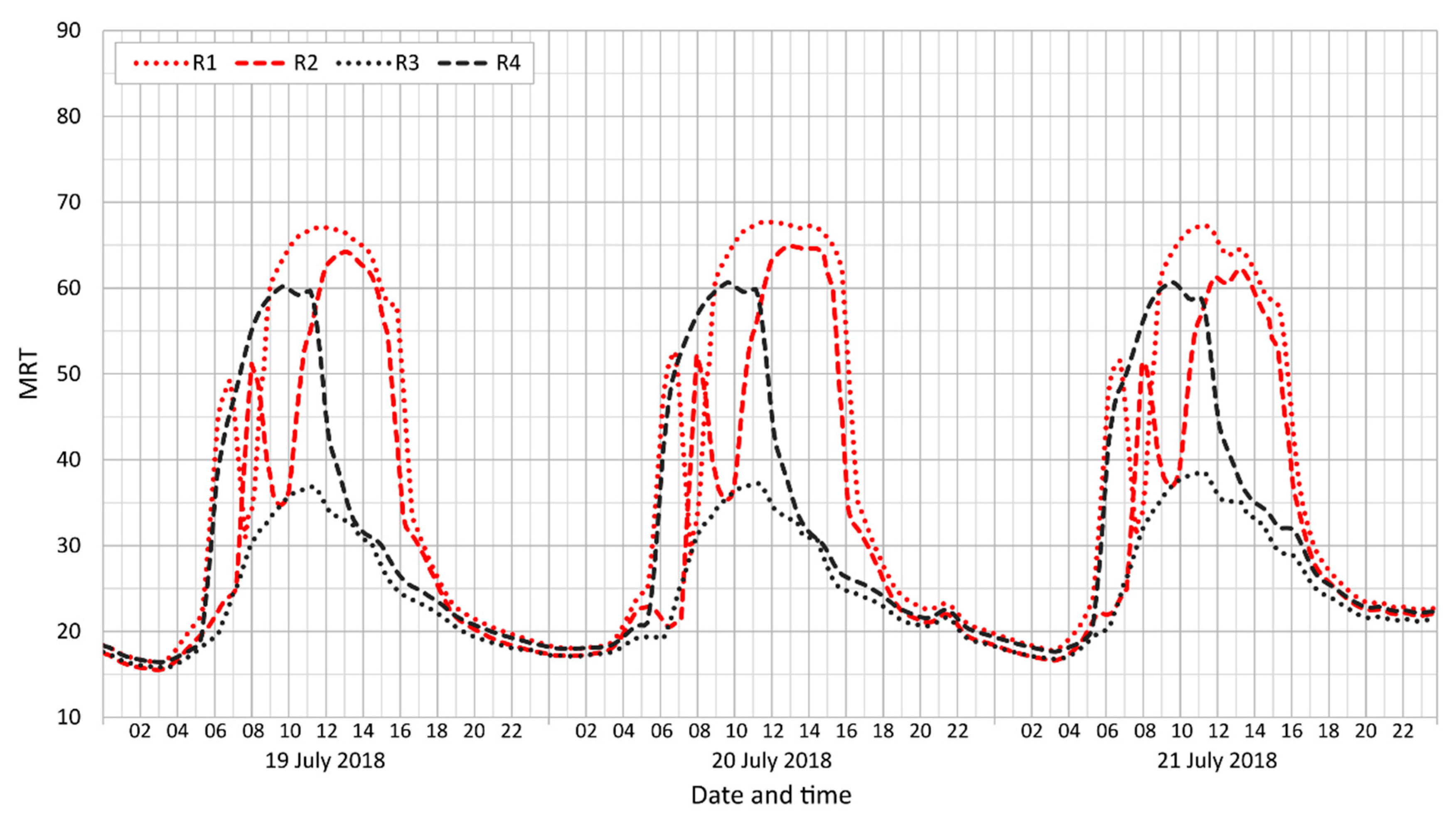
5.2.2. Courtyards
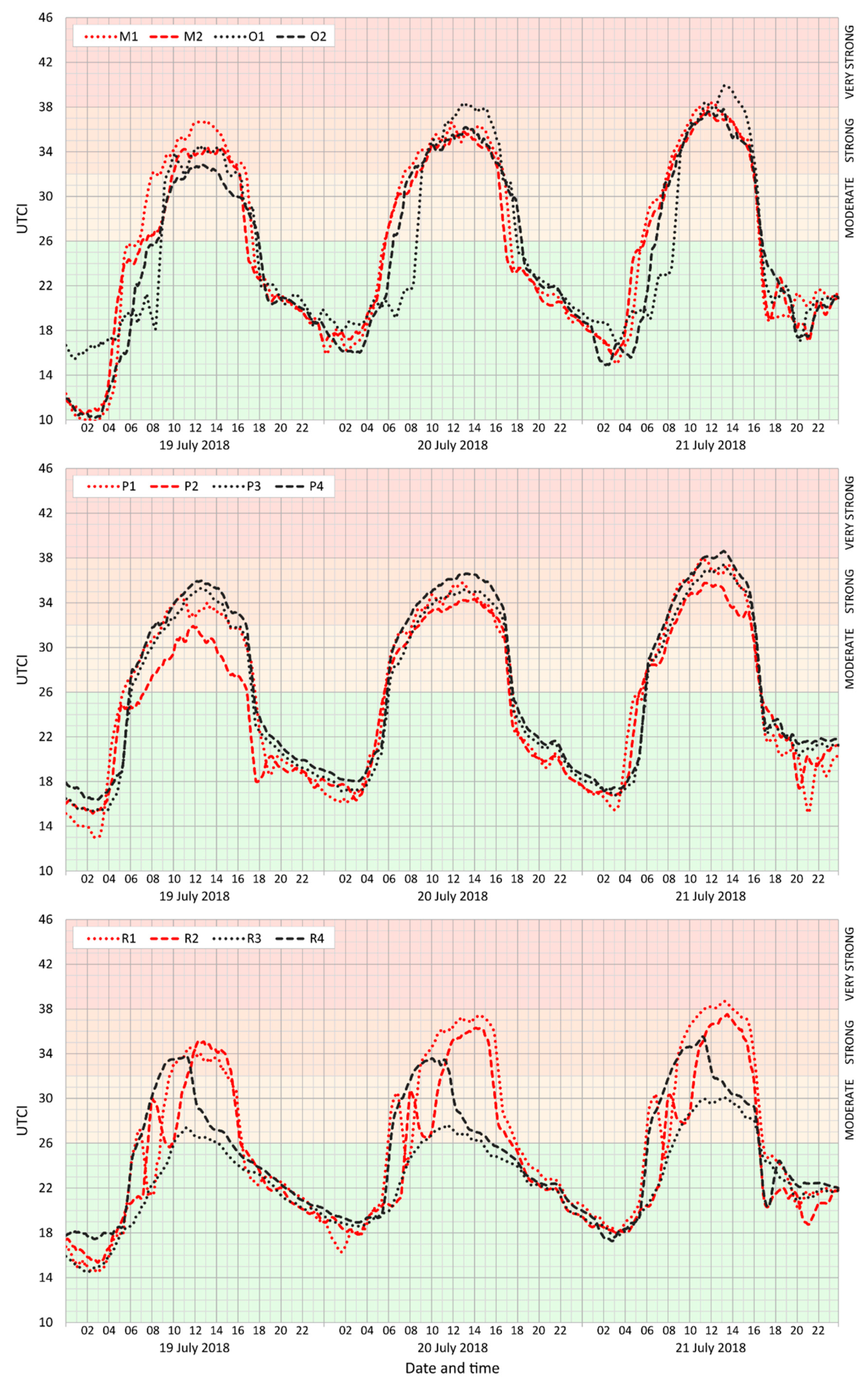
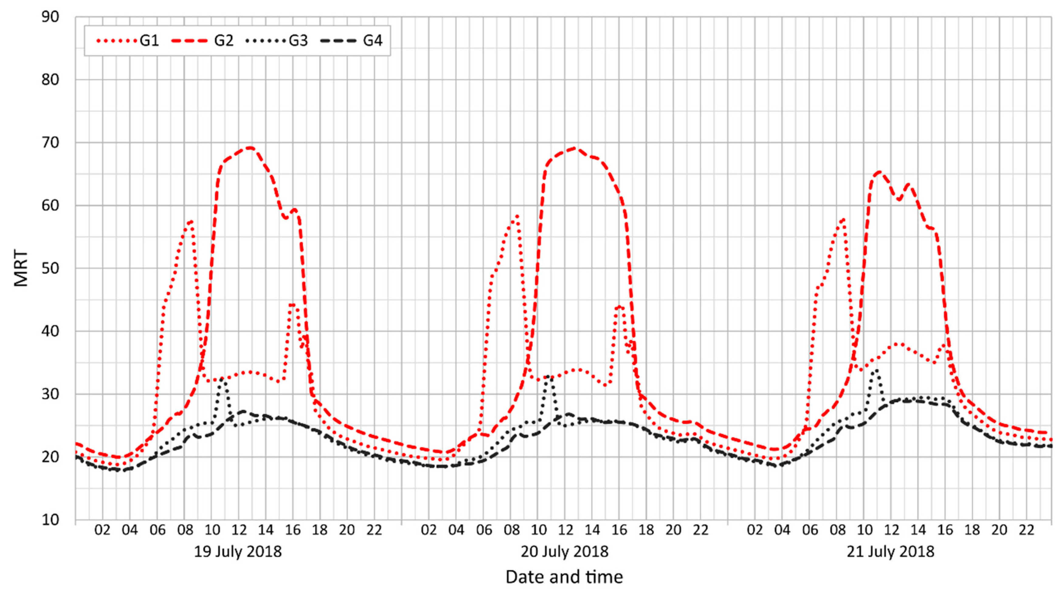
5.2.3. Public Places
6. Discussion and Conclusions
6.1. Thermal Exposure in a Moderate-Climate Urban Environment
6.2. Model and Simulation Limits, Validation, and Further Development
Author Contributions
Funding
Informed Consent Statement
Data Availability Statement
Acknowledgments
Conflicts of Interest
Abbreviations
| BIO | biometeorology module in PALM |
| BEM | building energy model |
| H | relative humidity (%) |
| LAD | leaf area density |
| LES | large-eddy simulation |
| LSM | land surface module |
| LW | long-wave (e.g., radiation) |
| MRT | mean radiant temperature |
| PALM | parallelized large-eddy simulation model |
| PET | physiologically equivalent temperature |
| RTM | radiative transfer model |
| SW | short-wave (e.g., radiation) |
| T | air temperature (2 m; °C) |
| UTCI | Universal Thermal Climate Index |
| v | wind speed (m·s−1) |
| WRF | Weather Research and Forecasting model |
Appendix A

Appendix B


Appendix C

Appendix D


References
- Parsons, K. Human Thermal Environments: The Effects of Hot, Moderate, and Cold Environments on Human Health, Comfort, and Performance, 3rd ed.; CRC Press: Boca Raton, FL, USA, 2014; 635p. [Google Scholar] [CrossRef]
- Potchter, O.; Cohen, P.; Lin, T.P.; Matzarakis, A. Outdoor human thermal perception in various climates: A comprehensive review of approaches, methods and quantification. Sci. Total Environ. 2018, 631, 390–406. [Google Scholar] [CrossRef] [PubMed]
- Revi, A.; Satterthwaite, D.E.; Aragón-Durand, F.; Corfee-Morlot, J.; Kiunsi, R.B.R.; Pelling, M.; Roberts, D.C.; Solecki, W. Urban areas. In Climate Change 2014: Impacts, Adaptation, and Vulnerability. Part A: Global and Sectoral Aspects; Contribution of Working Group II to the Fifth Assessment Report of the Intergovernmental Panel on Climate Change; Field, C.B., Barros, V.R., Dokken, D.J., Mach, K.J., Mastrandrea, M.D., Bilir, T.E., Chatterjee, M., Ebi, K.L., Estrada, Y.O., Genova, R.C., et al., Eds.; Cambridge University Press: Cambridge, UK; New York, NY, USA, 2014; pp. 535–612. [Google Scholar] [CrossRef] [Green Version]
- Hondula, D.M.; Balling, R.C., Jr.; Andrade, R.; Krayenhoff, S.; Middel, A.; Urban, A.; Georgescu, M.; Sailor, D.J. Biometeorology for cities. Int. J. Biometeorol. 2017, 61, 59–69. [Google Scholar] [CrossRef] [PubMed]
- Chen, L.; Ng, E. Outdoor thermal comfort and outdoor activities: A review of research in the past decade. Cities 2012, 29, 118–125. [Google Scholar] [CrossRef]
- Urban, A.; Kyselý, J. Comparison of UTCI with other thermal indices in the assessment of heat and cold effects on cardiovascular mortality in the Czech Republic. Int. J. Environ. Res. Public Health 2014, 11, 952–967. [Google Scholar] [CrossRef] [PubMed] [Green Version]
- Vanos, J.K.; Baldwin, J.W.; Jay, O.; Ebi, K.L. Simplicity lacks robustness when projecting heat-health outcomes in a changing climate. Nat. Commun. 2020, 11, 1–5. [Google Scholar] [CrossRef]
- Vanos, J.K.; Warland, J.S.; Gillespie, T.J.; Kenny, N.A. Review of the physiology of human thermal comfort while exercising in urban landscapes and implications for bioclimatic design. Int. J. Biometeorol. 2010, 54, 319–334. [Google Scholar] [CrossRef]
- Demuzere, M.; Orru, K.; Heidrich, O.; Olazabal, E.; Geneletti, D.; Orru, H.; Bhave, A.G.; Mittal, N.; Feliu, E.; Faehnle, M. Mitigating and adapting to climate change: Multi-functional and multi-scale assessment of green urban infrastructure. J. Environ. Manag. 2014, 146, 107–115. [Google Scholar] [CrossRef]
- Geletič, J.; Lehnert, M.; Savić, S.; Milošević, D. Modelled spatiotemporal variability of outdoor thermal comfort in local climate zones of the city of Brno, Czech Republic. Sci. Total Environ. 2018, 624, 385–395. [Google Scholar] [CrossRef]
- Stewart, I.D. Why should urban heat island researchers study history? Urban Clim. 2019, 30, 100484. [Google Scholar] [CrossRef]
- Maronga, B.; Banzhaf, S.; Burmeister, C.; Esch, T.; Forkel, R.; Fröhlich, D.; Fuka, V.; Gehrke, K.F.; Geletič, J.; Giersch, S.; et al. Overview of the PALM model system 6.0. Geosci. Model Dev. 2020, 13, 1335–1372. [Google Scholar] [CrossRef]
- Jendritzky, G.; Havenith, G.; Weihs, P.; Batchvarova, E. Towards a Universal Thermal Climate Index UTCI for Assessing the Thermal Environment of the Human Being; Final Report COST Action; COST (European Cooperation in Science and Technology): Brussels, Belgium, 2009; pp. 1–26. [Google Scholar]
- Jendritzky, G.; de Dear, R.; Havenith, G. UTCI—Why another thermal index? Int. J. Biometeorol. 2012, 56, 421–428. [Google Scholar] [CrossRef] [Green Version]
- Resler, J.; Eben, K.; Geletič, J.; Krč, P.; Rosecký, M.; Sühring, M.; Belda, M.; Fuka, V.; Halenka, T.; Huszár, P.; et al. Validation of the PALM model system 6.0 in real urban environment; case study of Prague-Dejvice, Czech Republic. Geosci. Model Dev. Discuss. 2020. [Google Scholar] [CrossRef]
- Fischereit, J.; Schlünzen, K.H. Evaluation of thermal indices for their applicability in obstacle-resolving meteorology models. Int. J. Biometeorol. 2018, 62, 1887–1900. [Google Scholar] [CrossRef] [PubMed] [Green Version]
- Fanger, P.O. Thermal Comfort; McGraw-Hill Book Company: New York, NY, USA, 1970. [Google Scholar] [CrossRef]
- Höppe, P. The physiological equivalent temperature—A universal index for the biometeorological assessment of the thermal environment. Int. J. Biometeorol. 1999, 43, 71–75. [Google Scholar] [CrossRef] [PubMed]
- Stewart, I.D. A systematic review and scientific critique of methodology in modern urban heat island literature. Int. J Climatol. 2011, 31, 200–217. [Google Scholar] [CrossRef]
- Voogt, J.A.; Oke, T.R. Thermal remote sensing of urban climates. Remote Sens. Environ. 2003, 86, 370–384. [Google Scholar] [CrossRef]
- Chandler, T.J. Selected Bibliography on Urban Climate; WMO Technical Note No. 276; WMO: Geneva, Switzerland, 1970; p. 392. [Google Scholar]
- Oke, T.R. Review of Urban Climatology, 1968–1973; WMO Technical Note No. 134; WMO: Geneva, Switzerland, 1974; p. 152. [Google Scholar]
- Oke, T.R. Review of Urban Climatology, 1973–1976; WMO Technical Note No. 169; WMO: Geneva, Switzerland, 1979; p. 539. [Google Scholar]
- Yoshino, M. Development of urban climatology and problems today. Energy Build. 1990, 15, 1–10. [Google Scholar] [CrossRef]
- Arnfield, A.J. Two decades of urban climate research: A review of turbulence, exchanges of energy and water, and the urban heat island. Int. J. Climatol. 2003, 23, 1–26. [Google Scholar] [CrossRef]
- Mills, G. Urban climatology: History, status and prospects. Urban Clim. 2014, 10, 479–489. [Google Scholar] [CrossRef]
- Oke, T.R.; Mills, G.; Christen, A.; Voogt, J.A. Urban Climates; Cambridge University Press: Cambridge, UK, 2017. [Google Scholar] [CrossRef] [Green Version]
- Kántor, N.; Kovács, A.; Lin, T.P. Looking for simple correction functions between the mean radiant temperature from the “standard black globe” and the “six-directional” techniques in Taiwan. Theor. Appl. Climatol. 2015, 121, 99–111. [Google Scholar] [CrossRef]
- Schnell, I.; Potchter, O.; Yaakova, Y.; Epstein, Y. Human exposure to environmental health concern by types of urban environment: The case of Tel Aviv. Environ. Pollut. 2016, 208, 58–65. [Google Scholar] [CrossRef] [PubMed]
- Schlünzen, K.H.; Hinneburg, D.; Knoth, O.; Lambrecht, M.; Leitl, B.; López, S.; Lüpkes, C.; Panskus, H.; Renner, E.; Schatzmann, M.; et al. Flow and transport in the obstacle layer: First results of the micro-scale model MITRAS. J. Atmos. Chem. 2003, 44, 113–130. [Google Scholar] [CrossRef]
- Bruse, M. Envi-Met 3.0: Updated Model Overview; University of Bochum: Bochum, Germany, 2004; Available online: http://www.envi-met.net/documents/papers/overview30.pdf (accessed on 20 November 2020).
- Sievers, U. Das Kleinskalige Strömungsmodell MUKLIMO_3 Teil 1: Theoretische Grundlagen, PC-Basisversion und Validierung; Berichte des Deutschen Wetterdienstes, Band 240; Deutschen Wetterdienstes: Offenbach, Germany, 2008. [Google Scholar]
- Sievers, U. Das Kleinskalige Strömungsmodell MUKLIMO_3 Teil 2: Thermodynamische Erweiterungen; Berichte des Deutschen Wetterdienstes, Band 248; Deutschen Wetterdienstes: Offenbach, Germany, 2016. [Google Scholar]
- De Ridder, K.; Lauwaet, D.; Maiheu, B. UrbClim—A fast urban boundary layer climate model. Urban Clim. 2015, 12, 21–48. [Google Scholar] [CrossRef] [Green Version]
- Resler, J.; Krč, P.; Belda, M.; Juruš, P.; Benešová, N.; Lopata, J.; Vlček, O.; Damašková, D.; Eben, K.; Derbek, P.; et al. PALM-USM v1.0: A new urban surface model integrated into the PALM large-eddy simulation model. Geosci. Model Dev. 2017, 10, 3635–3659. [Google Scholar] [CrossRef] [Green Version]
- Krč, P.; Resler, J.; Fuka, V.; Sühring, M.; Salim, M. Radiative Transfer Model 3.0 integrated into the PALM model system 6.0. Geosci. Model Dev. Discuss. 2020. [Google Scholar] [CrossRef]
- Fröhlich, J.; von Terzi, D. Hybrid LES/RANS methods for the simulation of turbulent flows. Prog. Aerosp. Sci. 2008, 44, 349–377. [Google Scholar] [CrossRef]
- Fröhlich, D.; Matzarakis, A. Calculating human thermal comfort and thermal stress in the PALM model system 6.0. Geosci. Model Dev. 2020, 13, 3055–3065. [Google Scholar] [CrossRef]
- Geletič, J.; Lehnert, M.; Jurek, M. Spatiotemporal variability of air temperature during a heat wave in real and modified landcover conditions: Prague and Brno (Czech Republic). Urban Clim. 2020, 31, 100588. [Google Scholar] [CrossRef]
- Wicker, L.J.; Skamarock, W.C. Time-Splitting Methods for Elastic Models Using Forward Time Schemes. Mon. Weather Rev. 2002, 130, 2088–2097. [Google Scholar] [CrossRef]
- Hackbusch, W. Introductory Model Problem. In Multigrid Method and Application; Graham, R.L., Jolla, L., Eds.; Springer: Berlin/Heidelberg, Germany, 1985; pp. 17–39. [Google Scholar] [CrossRef]
- Maronga, B.; Gryschka, M.; Heinze, R.; Hoffmann, F.; Kanani-Sühring, F.; Keck, M.; Ketelsen, K.; Letzel, M.O.; Sühring, M.; Raasch, S. The Parallelized Large-Eddy Simulation Model (PALM) version 4.0 for atmospheric and oceanic flows: Model formulation, recent developments, and future perspectives. Geosci. Model Dev. 2015, 8, 2515–2551. [Google Scholar] [CrossRef] [Green Version]
- Fiala, D.; Havenith, G.; Bröde, P.; Kampmann, B.; Jendritzky, G. UTCI-Fiala multi-node model of human heat transfer and temperature regulation. Int. J. Biometeorol. 2012, 56, 429–441. [Google Scholar] [CrossRef] [PubMed] [Green Version]
- Havenith, G.; Fiala, D.; Błazejczyk, K.; Richards, M.; Bröde, P.; Holmér, I.; Rintamaki, H.; Benshabat, Y.; Jendritzky, G. The UTCI-clothing model. Int. J. Biometeorol. 2012, 56, 461–470. [Google Scholar] [CrossRef] [PubMed] [Green Version]
- Novák, M. Use of the UTCI in the Czech Republic. Geogr. Pol. 2013, 86, 21–28. [Google Scholar] [CrossRef]
- Mayer, H.; Holst, J.; Dostal, P.; Imbery, F.; Schindler, D. Human thermal comfort in summer within an urban street canyon in Central Europe. Meteorol. Z. 2008, 17, 241–250. [Google Scholar] [CrossRef]
- Kántor, N.; Unger, J. The most problematic variable in the course of human-biometeorological comfort assessment—The mean radiant temperature. Open Geosci. 2011, 3, 90–100. [Google Scholar] [CrossRef] [Green Version]
- Eliasson, I.; Knez, I.; Westerberg, U.; Thorsson, S.; Lindberg, F. Climate and behaviour in a Nordic city. Landsc. Urban Plan. 2007, 82, 72–84. [Google Scholar] [CrossRef]
- Lehnert, M.; Tokar, V.; Jurek, M.; Geletič, J. Summer thermal comfort in Czech cities: Measured effects of blue and green features in city centres. Int. J. Biometeorol. 2020. [Google Scholar] [CrossRef]
- Eliasson, I.; Offerle, B.; Grimmond, C.S.B.; Lindqvist, S. Wind fields and turbulence statistics in an urban street canyon. Atmos. Environ. 2006, 40, 1–16. [Google Scholar] [CrossRef]
- Tominaga, Y.; Mochida, A.; Yoshie, R.; Kataoka, H.; Nozu, T.; Yoshikawa, M.; Shirasawa, T. AIJ guidelines for practical applications of CFD to pedestrian wind environment around buildings. J. Wind Eng. Ind. Aerod. 2008, 96, 1749–1761. [Google Scholar] [CrossRef]
- Arinami, Y.; Akabayashi, S.; Tominaga, Y.; Sakaguchi, J. Performance evaluation of single-sided natural ventilation for generic building using large-eddy simulations: Effect of guide vanes and adjacent obstacles. Build. Environ. 2019, 164, 68–80. [Google Scholar] [CrossRef]
- Shirzadi, M.; Tominaga, Y.; Mirzaei, P.A. Experimental and Steady-RANS CFD Modelling of Cross-ventilation in Moderately-dense Urban Areas. Sustain. Cities Soc. 2020, 52, 101849. [Google Scholar] [CrossRef]
- Oke, T.R. Street design and urban canopy layer climate. Energy Build. 1988, 11, 103–113. [Google Scholar] [CrossRef]
- Kántor, N.; Égerházi, L.; Unger, J. Subjective estimation of thermal environment in recreational urban spaces—Part 1: Investigations in Szeged, Hungary. Int. J. Biometeorol. 2012, 56, 1075–1088. [Google Scholar] [CrossRef] [PubMed]
- Richards, K. Urban and rural dewfall, surface moisture, and associated canopy-level air temperature and humidity measurements for Vancouver, Canada. Bound. Layer Meteorol. 2005, 114, 143–163. [Google Scholar] [CrossRef]
- Fortuniak, K.; Kłysik, K.; Wibig, J. Urban–rural contrasts of meteorological parameters in Łódź. Theor. Appl. Climatol. 2006, 84, 91–101. [Google Scholar] [CrossRef]
- Lehnert, M.; Geletič, J.; Dobrovolný, P.; Jurek, M. Temperature differences among local climate zones established by mobile measurements: Two central European cities. Clim. Res. 2018, 75, 53–64. [Google Scholar] [CrossRef]
- Bokwa, A.; Geletič, J.; Lehnert, M.; Žuvela-Aloise, M.; Hollósi, B.; Gál, T.; Skarbit, N.; Dobrovolný, P.; Hajto, M.J.; Kielar, R.; et al. Heat load assessment in Central European cities using an urban climate model and observational monitoring data. Energy Build. 2019, 201, 53–69. [Google Scholar] [CrossRef]
- Dian, C.; Pongrácz, R.; Dezső, Z.; Bartholy, J. Annual and monthly analysis of surface urban heat island intensity with respect to the local climate zones in Budapest. Urban Clim. 2020, 31, 100573. [Google Scholar] [CrossRef]
- Mayer, H.; Höppe, P. Thermal comfort of man in different urban environments. Theor. Appl. Climatol. 1987, 38, 43–49. [Google Scholar] [CrossRef]
- Mayer, H.; Kuppe, S.; Holst, J.; Imbery, F.; Matzarakis, A. Human Thermal Comfort below the Canopy of Street Trees on a Typical Central European Summer Day; Berichte des Meteorologischen Instituts der Albert-Ludwigs-Universität Freiburg; University of Freiburg: Breisgau, Germany, 2009; pp. 211–219. [Google Scholar]
- Belda, M.; Eben, K.; Fuka, V.; Geletič, J.; Kanani-Sühring, F.; Krč, P.; Maronga, B.; Resler, J.; Benešová, N.; Sühring, M.; et al. Sensitivity analysis of the PALM model system 6.0 in the urban environment. Geosci. Model Dev. Discuss. 2020. [Google Scholar] [CrossRef]
- Oke, T.R. Initial Guidance to Obtain Representative Meteorological Observations at Urban Sites; World Meteorological Organization: Geneva, Switzerland, 2006; p. 47. [Google Scholar]
- Kántor, N.; Kovács, A.; Takács, Á. Small-scale human-biometeorological impacts of shading by a large tree. Open Geosci. 2016, 8, 231–245. [Google Scholar] [CrossRef] [Green Version]
- Coutts, A.M.; White, E.C.; Tapper, N.J.; Beringer, J.; Livesley, S.J. Temperature and human thermal comfort effects of street trees across three contrasting street canyon environments. Theor. Appl. Climatol. 2016, 124, 55–68. [Google Scholar] [CrossRef]
- Middel, A.; Krayenhoff, E.S. Micrometeorological determinants of pedestrian thermal exposure during record-breaking heat in Tempe, Arizona: Introducing the MaRTy observational platform. Sci. Total Environ. 2019, 687, 137–151. [Google Scholar] [CrossRef] [PubMed]
- Gulyás, Á.; Unger, J.; Matzarakis, A. Assessment of the microclimatic and human comfort conditions in a complex urban environment: Modelling and measurements. Build. Environ. 2006, 41, 1713–1722. [Google Scholar] [CrossRef]
- Lindberg, F.; Grimmond, C.S.B. The influence of vegetation and building morphology on shadow patterns and mean radiant temperatures in urban areas: Model development and evaluation. Theor. Appl. Climatol. 2011, 105, 311–323. [Google Scholar] [CrossRef]
- Takács, Á.; Kiss, M.; Hof, A.; Tanács, E.; Gulyás, Á.; Kántor, N. Microclimate modification by urban shade trees–an integrated approach to aid ecosystem service based decision-making. Procedia Environ. Sci. 2016, 32, 97–109. [Google Scholar] [CrossRef] [Green Version]
- Morakinyo, T.E.; Kong, L.; Lau, K.K.L.; Yuan, C.; Ng, E. A study on the impact of shadow-cast and tree species on in-canyon and neighborhood’s thermal comfort. Build. Environ. 2017, 115, 1–17. [Google Scholar] [CrossRef]
- Lee, H.; Mayer, H.; Kuttler, W. Impact of the spacing between tree crowns on the mitigation of daytime heat stress for pedestrians inside E-W urban street canyons under Central European conditions. Urban For. Urban Green. 2020, 48, 126558. [Google Scholar] [CrossRef]
- Bongardt, B. Stadtklimatologische Bedeutung kleiner Parkanlagen: Dargestellt am Beispiel des Dortmunder Westparks (Essener Ökologische Schriften); Westarp Wissenschaften: Hohenwarsleben, Germany, 2006; Volume 24, 268p, ISBN 978-3894321109. [Google Scholar]
- Müller, N.; Kuttler, W.; Barlag, A.B. Counteracting urban climate change: Adaptation measures and their effect on thermal comfort. Theor. Appl. Climatol. 2014, 115, 243–257. [Google Scholar] [CrossRef] [Green Version]
- Lehnert, M. The soil temperature regime in the urban and suburban landscapes of Olomouc, Czech Republic. Morav. Geogr. Rep. 2013, 21, 27–36. [Google Scholar] [CrossRef] [Green Version]
- Resler, J.; Eben, K.; Geletič, J.; Krč, P.; Rosecký, M.; Sühring, M.; Belda, M.; Fuka, V.; Halenka, T.; Huszár, P.; et al. PALM 6.0 revision 4508; Leibniz University: Hannover, Germany, 2020. [Google Scholar] [CrossRef]
- Kántor, N.; Chen, L.; Gál, C.V. Human-biometeorological significance of shading in urban public spaces—Summertime measurements in Pécs, Hungary. Landsc. Urban Plan. 2018, 170, 241–255. [Google Scholar] [CrossRef]


Publisher’s Note: MDPI stays neutral with regard to jurisdictional claims in published maps and institutional affiliations. |
© 2021 by the authors. Licensee MDPI, Basel, Switzerland. This article is an open access article distributed under the terms and conditions of the Creative Commons Attribution (CC BY) license (http://creativecommons.org/licenses/by/4.0/).
Share and Cite
Geletič, J.; Lehnert, M.; Krč, P.; Resler, J.; Krayenhoff, E.S. High-Resolution Modelling of Thermal Exposure during a Hot Spell: A Case Study Using PALM-4U in Prague, Czech Republic. Atmosphere 2021, 12, 175. https://0-doi-org.brum.beds.ac.uk/10.3390/atmos12020175
Geletič J, Lehnert M, Krč P, Resler J, Krayenhoff ES. High-Resolution Modelling of Thermal Exposure during a Hot Spell: A Case Study Using PALM-4U in Prague, Czech Republic. Atmosphere. 2021; 12(2):175. https://0-doi-org.brum.beds.ac.uk/10.3390/atmos12020175
Chicago/Turabian StyleGeletič, Jan, Michal Lehnert, Pavel Krč, Jaroslav Resler, and Eric Scott Krayenhoff. 2021. "High-Resolution Modelling of Thermal Exposure during a Hot Spell: A Case Study Using PALM-4U in Prague, Czech Republic" Atmosphere 12, no. 2: 175. https://0-doi-org.brum.beds.ac.uk/10.3390/atmos12020175