Road Emissions in London: Insights from Geographically Detailed Classification and Regression Modelling

Abstract

Greenhouse gases and air pollutant emissions originating from road transport continues to rise in the UK, indicating a significant contribution to climate change and negative impacts on human health and ecosystems. However, emissions are usually estimated at aggregated levels, and on many occasions roads of minor importance are not taken into account, normally due to lack of traffic counts. This paper presents a methodology enabling estimation of air pollutants and CO₂ for each street segment in the Greater London area. This is achieved by applying a hybrid probabilistic classification–regression approach on a set of variables believed to affect traffic volumes and utilizing emission factors. The output reveals pollution hot spots and the effects of open spaces in a spatially rich dataset. Considering the disaggregated approach, the methodology can be used to facilitate policy making for both local and national aggregated levels.

1. Introduction

Recent data show that despite a decrease in the UK’s total greenhouse gas (GHG) emissions by 32% since the 1990s, emissions from road transport have increased by 6% during the same period [1]. In fact, road transport alone makes up approximately 20% of the UK’s total GHG emissions [1] with 92% of emissions originating from transport—and in particular CO₂ [2]—having global impacts and contributing to climate change [3]. In addition, road transport is a significant source of air pollutants—such as nitrogen oxides (NO_x), particulate matter (PM) and carbon monoxide (CO)—contributing up to 80% of total transport pollutant emissions [4]. These pollutants are responsible for negative impacts on human health and ecosystems [5] and even though there has been a significant reduction in emissions, damage to human health can occur even at low levels [6,7].

To date, a number of studies have focused on the estimation of GHG and air pollutant emissions from the road transport sector to further understand environmental and health implications and facilitate policy making. However, numerous limitations and diverse results are observed, usually depending on the selected model and data availability, subject to area/country of application. For example, emissions are usually estimated at an aggregated level such as national, regional or city-wide e.g., [8,9,10]. Therefore, conclusions about local impacts cannot be drawn. In addition, some countries—such as the UK—estimate emissions on roads of minor importance based on average regional flows [11,12], due to lack of traffic measurements on these roads. Considering that minor roads are less crowded, but make up 87% of total road length in the UK [13], the aforementioned methodological approach implies incomplete and unreliable emission estimation across the full extent of the road network.

Consequently, traffic flow estimation for roads where data is not available has been investigated in numerous studies, where several influencing factors have been incorporated. In particular, estimation of annual average daily traffic (AADT)—a measure of traffic flow defined as the average traffic volume of a street segment on an average day in the year [14]—has been investigated in studies on motorised, e.g., [15] and non-motorised transport e.g., [16,17]. However, estimation is mainly conducted on total AADT while the volumes of specific vehicle types—and the associated emissions—in the road network is still to a great extent unexplored. Furthermore, research is mainly focused on AADT estimation on major roads e.g., [18] with only a few studies incorporating minor roads e.g., [19,20]. The latter is considered fundamental to estimate traffic flows and related emissions for various vehicle types, and facilitate policy making and urban and environmental planning.

The aim of this paper is to estimate specific air pollutants and GHGs (PM_2.5, NO_x, CO and CO₂) at a detailed level of analysis (i.e., link/street segment) for all roads—major and minor—in the Greater London area, while addressing and potentially overcoming the identified limitations of the modelling implemented so far. To achieve this, we present a two-fold methodological approach based on classification and regression models, where emissions are estimated for all available vehicle types. The method incorporates data from different sources partially manipulated within a geographic information system (GIS). Considering the outputs are at detailed local levels, we envisage it can be used to identify both hot spots of air pollution exposure and GHG emissions, as well as to estimate total (i.e., aggregated) emissions.

The paper is presented in 7 sections. Section 2 introduces road transport emission modelling approaches and respective applications. Section 3 presents the datasets used and Section 4 describes the methodological steps followed to estimate emissions. Section 5 presents the outcomes from the modelling process, while in Section 6 we discuss these results. Finally, Section 7 concludes on the outcomes and investigates potential future studies to improve our work.

2. Literature Review

Estimation of GHG and air pollutant emissions from road transport can be conducted with the use of various emission models classified depending on geographic scale of application, methodological approach and generic model type [21]. In particular, road transport emission models can be classified into static and dynamic, with each type exhibiting advantages and disadvantages, mainly related to data availability, and required computer processing as well as the scale of application. Static and dynamic models are further classified into (1) traffic situation, (2) instantaneous, (3) average speed and (4) aggregate emission factor models [22]. The first three classes are also introduced in [23] and are generally accepted and widely used in the literature, although some studies use different classifications. For example, [21] introduce variations of average speed and instantaneous models, [24] classify the models based on the type of emissions, while [25] do so based on input data, study scale and type of pollutants being modelled. The major requirement for all emissions models is activity (i.e., traffic) data, extracted from transport models.

Traffic situation models estimate emissions related to particular traffic patterns, using emission factors for each situation, with situations defined in terms of road type, area type, speed limit and congestion level where a specific traffic patterns occurs [26]. These models require information on vehicle kilometres travelled (VKT) and on the traffic situation applied to each road link [27]. Incorporation of traffic situation models can be found in a number of cases, such as the Handbook of Emission Factors for Road Transport (HBEFA) database which provides emission factors based on defined traffic situations [28]. HBEFA has been used by [8] to estimate nitrogen oxides (NO_x) in Madrid and [29] to estimate carbon monoxide (CO), carbon dioxide (CO₂) and NO_x emissions with both studies concluding that the model overestimates emissions. By contrast, [30] testing HBEFA on CO concludes that the model underestimates emissions. The Assessment and Reliability of Transport Emissions Models and Inventory Systems (ARTEMIS) is another traffic situation model [31,32] consisting of a collection of sub-models [33]. The model has been used by [34] to measure compound emissions for diesel and petrol vehicles and by [35] for CO, HC and NO_x for two wheeled vehicles. ARTEMIS emission factors were also used by [36] to estimate CO₂ in Sweden.

Instantaneous emission models relate emission rates to vehicle operational modes [27] so that a traffic simulation module provides vehicle operation data and the emission module assigns an emission factor to each combination of instantaneous speed and acceleration rates [22]. The Passenger car and Heavy duty vehicle Emission Model (PHEM) is the most significant example of an instantaneous model [25] based on parameters from real driving conditions considering factors such as road gradients and vehicle loading [37]. PHEM is incorporated in the HBEFA model, providing evaporation emission factors for air pollutants and CO₂ emissions [28].

Average speed models use average rather than instantaneous emission factors varying according to the average speed of a vehicle [21] and applying to a street segment or an entire journey [26]. The Computer Program to calculate Emissions from Road Transport (COPERT) is the most widely used average speed tool for air pollutants and GHGs, where emission factors are expressed as function of the average speed over a complete driving cycle [38] and can also be used to provide distance-based emission factors. COPERT has been used and integrated in numerous studies and models, such as the National Atmospheric Emissions Inventory (NAEI) in the UK, providing emission maps based on spatial datasets and traffic count data [11]. In other studies COPERT has been used by [39] to estimate CO₂, NO_x and PM_2.5 on major roads in Belgium and [9] to assess the impact of a shift from private cars and motorcycles to public transport, and a shift from conventional fuel use to natural gas on GHG and air pollutant emissions in Malaysia. In China, [40] used the model to estimate emissions from passenger cars, for three future scenarios, while in the UK [41] used COPERT to predict impacts of CO₂, NO_x and black carbon based on different traffic management measures in Glasgow.

Other less common models for estimating emissions from road transport in the UK include: (1) the UK Transport Carbon Model (UKTCM) developed to provide annual projections for all passenger and freight transport supply and demand as well as estimate CO₂, CO, NO_x, SO₂, total hydrocarbons (THC) and PM emissions [42]. (2) The Background, Road and Urban Transport modelling of Air quality Limit values (BRUTAL) model [43], which is based on the previous Abatement Strategies Assessment Model (ASAM) [44] and the UK Integrated Assessment Model (UKIAM) [45] using GIS and incorporating datasets extracted from NAEI and COPERT. A different approach based on dispersion kernels is incorporated in the SHERPA-city application developed by [46] and applied in Madrid to estimate NO_x and NO₂ concentrations. As an alternative and sometimes combined with the set models discussed, a different methodological approach has been applied. In particular, GHG and air pollutant emissions can be estimated by multiplying emission factors with activity data (e.g., annual vehicle kilometres travelled), similar to the methodology used in NAEI to estimate hot exhaust emissions [47]. In fact, VKT is also an essential input for the COPERT model [48] and can be calculated by multiplying AADT by the length of each link [49], an essential indicator for accurate VKT calculation [50]. This approach has been used in [10] to estimate GHG, NO_x, CO and SO₂ in Mauritius where traffic counts (i.e., AADT) for all road classes are split by fuel type and fuel consumption is calculated by vehicle type and road class. Similarly, [51] estimate NO, CO₂, SO, PM and CO for a particular road in Indonesia and [52] calculated VKT from traffic counts to estimate CO, NO_x, PM_2.5 and volatile organic compounds (VOC) emitted from trucks on major roads in a Korean metropolitan area. [53] also utilised traffic counts to calculate VKT and emissions factors for each fuel and vehicle type to estimate CO₂ in Dhaka, Bangladesh and [54] estimated road transport emissions from VKT based on AADT, to distribute emissions along the road network in Salt Lake City, Utah. Finally, [55] used AADT values to calculate VKT and estimate PM_2.5, NO_x and HC emissions for each road link in the Republic of Ireland.

3. Data

To estimate emissions, we utilize datasets from different sources. For activity data, we use the dataset presented in [56]. This spatial dataset contains traffic count points across England and Wales for four road classes—‘A’, ‘B’, ‘C’ and ‘U’. For each count point, AADT values for five different vehicle types (cars and taxis, buses, light goods vehicles (LGVs), heavy goods vehicles (HGVs) and two-wheeled vehicles) are provided, coupled with a number of land use, socioeconomic, roadway and public transport characteristics in the vicinity (The vicinity around each point is defined by service areas—i.e., buffers around each point taking into account the road network—thus considering the actual distance driven by each vehicle.) of each point considered as factors affecting AADT. The attributes are shown in

Table A1. Attributes for each count point.

Variable	Description
1. Urban/Rural	Whether a count point is located at urban or rural environment
2. Distance to Urban Area	Distance of count point to the edge of the nearest edge of spatial polygon indicating urban area
3. Distance to Major Urban Area 1	Distance of count point to the edge of the nearest edge of spatial polygon indicating Major urban area 1
4. Distance to Urban Area Centroid	Distance of count point to the geometrical centroid of the nearest spatial polygon indicating urban area—indicating urban (city/town/village) centre
5. Distance to Major Urban Area 1 Centroid	Distance of count point to the geometrical centroid of the nearest spatial polygon indicating major urban area 1—indicating major urban (city) centre
6. Toll Road	Whether a count point is located on a road with tolls
7. Ring Road	Whether the count point is located on a ring road
8. Road Nature	Whether the count point is located on a single or dual carriageway, slip road or roundabout
9. Road Category	Whether the point is located on a primary or trunk road (mainly for higher class roads) in an urban or rural area
10. Junction Accessibility	Whether the point is located on a road with access to motorway within the specified service area
11. Bus Stops	Number of bus stops within the specified service area
12. Bus Stations	Number of bus stations within the specified service area
13. Train Accessibility	Indicating train station accessibility within the LSOA 2 where the count point is located.
14. Population	Total population of a count point’s adjacent LSOAs 2
15. Population Density	Average population density of a count point’s adjacent LSOAs 2
16. Workplace Population	Total number of registered employed people of a count point’s adjacent LSOAs 2
17. Workplace Population Density	Average of registered employers’ density around a count points’ adjacent LSOAs 2
18. Workplace plus Population Density	Average workplace plus population density of a count point’s adjacent LSOAs 2
19. Income	Average median income of a count point’s adjacent LSOAs 2
20. Households	Total number of households of a count point’s adjacent LSOAs 2
21. Registered Vehicles	Total number of registered cars and vans of a count point’s adjacent LSOAs 2
22. Charging Points	Number of charging points within each service area
23. Ports	Whether there is a port within the specified service area around the count point
24. Airports	Whether there is an airport within the specified service area around the count point
25. Research, Education and Training	Total number of Schools, Colleges, Libraries, Universities, Language and Music Schools, etc. within the specified service area
26. Factories, Workshops and Industrial Activity	Total number of Energy Production Facilities, Factories, Workshops, Mines, Oil Fields, Recycling Plants, Shipyards, Scrap Yards within the specified service area
27. Healthcare	Number of Hospitals, GPs, Surgeries, Clinics within the specified service area
28. Leisure	Number of Public Houses, Bars, Nightclubs, Restaurants, Art Galleries, Cinemas and Theatres, Coffee shops within the specified service area
29. Office and Business Space	Number of Offices, Banks, Business Units within the specified service area
30. Public Services, Infrastructure and Buildings	Number of Post Offices, Community Centres, Police and Fire Stations, Prisons, Courts within the specified service area
31. Shops, Stalls, Kiosks and Markets	Number of Shops, Kiosks, Showrooms, Stores within the specified service area
32. Super/Hyper Stores	Number of Superstores, Malls within the specified service area
33. Sport	Number of Stadia, Sport Centres, Golf Courses, Tennis Centres, Football Grounds within the specified service area
34. Vacation Sites, Accommodation and Facilities	Number of Campsites, Caravan Sites, Hotels, Guest Houses, Holiday Units, Hostels, Motels, Beach Houses within the specified service area
35. Petrol Stations	Number of Petrol Stations within the specified service area
36. Vehicle Infrastructure	Number of Vehicle Repair Workshop, Garages, Car Wash within the specified service area
37. Warehouse and Storage	Number of Warehouses, Depots, Storage Depots, Land Used for Storage within the specified service area
38. Parking Space	Number of Car/Vehicle Park Sites and Park Spaces, Motorcycle Bays within the specified service area
39. Animal Husbandry, Farming and Agriculture	Number of Aviaries, Farms, Animal Shelters, Stud Farms within the specified service area
40. Marine Infrastructure	Number of Mooring Sites, Quays, Wharfs, Lifeboat Stations, Marine Control Centres within the specified service area
41. Under (re)construction	Number of Properties and Premises Undergoing (re)Construction within the specified service area

¹ The six largest urban agglomerations in England and Wales (i.e., Greater London, West Midlands (Birmingham, Wolverhampton, Coventry), Greater Manchester, West Yorkshire (Leeds and Bradford), Tyneside (Newcastle and Sunderland) and Liverpool Urban Areas) as defined by [74]. ² Lower super output areas (LSOAs) indicate approximately 35,000 areas in England and Wales with a minimum of 1000 population.

in the Appendix A.

For each road class, meter count points are categorised in five subgroups generated by clustering. For each subgroup, six service areas are computed, containing information on attributes in the vicinity of the meter points. For each subgroup, the service area providing the best AADT estimation is selected in the final model. For more information on the process followed to build the dataset, the reader can refer to [56]. Sizes of service areas for each road class and Subgroup are shown in

Table 1. Service area by subgroup for each road class.

	Class	1	2	3	4	5
Subgroup
		Service Area Size (m)
A		800	1600	500	500	500
B		800	1000	800	800	2000
C		500	800	1000	800	2000
U		3200	800	1000	1000	2000

.

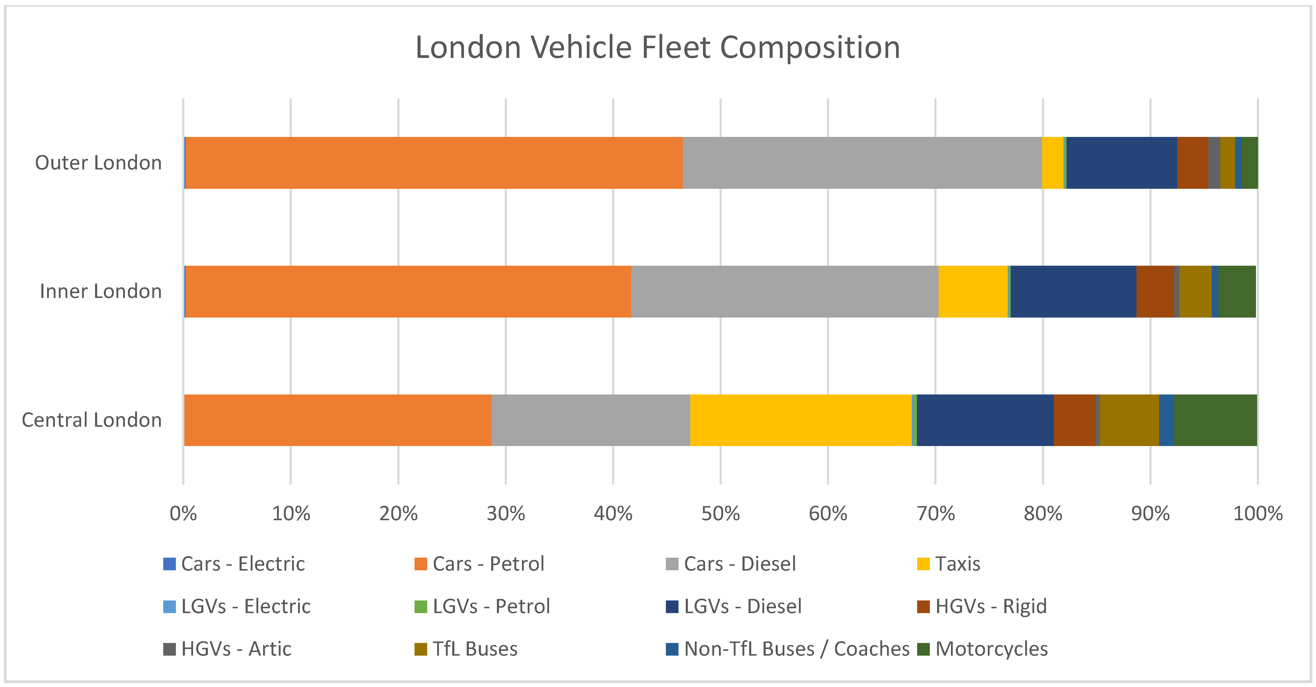
To account for all roads within the study area we also extract traffic count points for motorways from the Department for Transport, where again AADT for the same five vehicle categories are provided. In addition, we extract the London vehicle fleet composition (Figure 1) and air pollutant emission factors from the NAEI providing details for vehicle types and related fuels. CO₂ emission factors are extracted from The Department for Business, Energy and Industrial Strategy (BEIS).

4. Methodology

To estimate GHG and air pollutant emissions, one of the identified approaches has to be applied. However, from Section 2 it can be concluded that traffic situation and instantaneous emissions models cannot be utilised. Traffic situation models require detailed statistics for speed and a determination of each traffic situation for each road link [27] making these models unsuitable for extended application [22]. Also, instantaneous models are very rare [21] due to precision issues identified when measuring emissions, subject to vehicle operating conditions [57], as well as the need to include traffic simulation models, requiring a wide range of data which are difficult to obtain, calibrate and process [58]. By contrast, data required as inputs for average speed models are usually available and the models are comprehensive in terms of number of pollutants that can be modelled, vehicle types as well as influencing factors [26]. However, they do not take into account different driving behaviours and operational modes [59] usually resulting in different emissions and fuel consumption factors for the same speed [22]. Consequently, considering data availability we are estimating emissions in three major steps. First, we estimate traffic volumes—i.e., AADT—at locations where counts have not been measured. Second, we calculate VKT and finally, we use emission factors to estimate emissions following the methodologies presented in [10] and [55] among others.

4.1. Annual Average Daily Traffic (AADT) Estimation

To estimate traffic counts at unmeasured locations, we create “artificial” traffic counters at unmeasured street segments, by placing a point in the middle of each unmeasured segment using a GIS. For each new point, we create service areas of different sizes to take into account the land use, socioeconomic, roadway and public transport characteristics, based on service areas selected for each road class. For example, for count points on ‘A’ roads only service areas of 500, 800 and 1600 metres are considered as shown in Table 1. The process results in traffic counters with the same ID occurring multiple times in the dataset, with variable values different for each service area.

Then, each new point is allocated to the subgroup with most similar characteristics and the most suitable service area for each point based on the classification problems discussed below is identified. Moreover, the dataset provided already incorporates values for AADT—i.e., the value we aim to estimate—which has influenced the formation of subgroups [56].

To tackle these issues, we firstly select the points falling within the Greater London area, and we randomly split these—80% for training and 20% for testing—and exclude the dependent variable (i.e., AADT). We then use the training set to train three different classification algorithms (random forest (RF), gradient boosting machine (GBM), and K-nearest neighbour) and test the accuracy with the testing set using a confusion matrix. Among the three algorithms, GBM provided the highest classification accuracy (

Table A2. Classification accuracy.

Algorithm	A	B	C	U
RF	92.05%	50.00%	60.00%	67.57%
GBM	93.18%	50.00%	66.67%	70.27%
KNN	89.77%	37.50%	33.33%	64.86%

in the Appendix A) and it is, therefore, selected to classify the new points.

Finally, to account for points with repeated IDs we apply a GBM probabilistic classification [60] for all new points and service areas, so as to identify the probability of each point—and respective service area—belonging to each of the subgroups. For example, for ‘A’ roads if a service area of 800 metres is selected for a point, then it should be assigned to subgroup 1, but if a service area of 500 metres is selected, the point can belong to any of subgroups 3, 4 or 5 as shown in Table 1.

GBM is essentially an ensemble of “weak” prediction models—usually decision trees—aimed to improve accuracy by minimising the average value of the loss function $L\left(y_i,F\left(x\right)\right)$ on the training set [61], for a number of $M$ iterations [62], where $y_i$ is the observed value and $F\left(x\right)$ is the corresponding function The probability of a point belonging to a class is given by:

$$\mathbb{P}\left(y|x\right)=\frac{e^{\log \left(odds\right)}}{1+e^{\log \left(odds\right)}}$$

(1)

where $\log \left(odds\right)$ represents the odds of a point belonging to a class.

The algorithm, starts with a constant function:

$$F_0\left(x\right)=argmin{\displaystyle \sum }_{i=1}^{n}L\left(y_i,\gamma \right)$$

(2)

where $\gamma$ is the value for log(odds).

For each iteration (i.e., $m=1toM$), pseudo-residuals (i.e., the difference between the observed and predicted values) are computed:

$$r_i^m=-{\left[\frac{\partial L\left(y_i,F\left(x_i\right)\right)}{\partial F\left(x_i\right)}\right]}_{F\left(x\right)=F\left(m-1\right)\left(x\right)},{\forall }_i=1,2,\dots ,n$$

(3)

and a weak learner $h_m\left(x\right)$ is fitted to the residual values. Moreover, the parameter ${\gamma }_m$ is calculated as follows:

$${\gamma }_m=argmin{\displaystyle \sum }_{i=1}^{n}L\left(y_i,F_{\left(m-1\right)}\left(x_i\right)+\gamma h_m\left(x\right)\right)$$

(4)

and the model is updated as $F_m\left(x\right)=F_{\left(m-1\right)}\left(x\right)+{\gamma }_m{h}_m\left(x\right)$ where $h_m$ is the weak learner for iteration m and ${\gamma }_m$ the corresponding value extracted from Equation (4). Finally, the algorithm concludes in the final $F_M\left(x\right)$ output after M iterations.

After the new points are classified, to estimate AADT for each vehicle type, we apply RF regression within each subgroup using the existing points to train the algorithm and all the available independent variables. RF is applied for regression as the algorithm with the highest estimation accuracy for this model and dataset [56] based on mean absolute percentage error (MAPE) and root mean square error (RMSE). RF is a collection of decision trees based on bootstrapping and bootstrap aggregation [63,64] and the regression is performed as:

$$\widehat{f_{rf}^B}=\frac{1}{B}{\displaystyle \sum }_{b=1}^B{T}_b\left(x\right)$$

(5)

where: $B$ is the number of trees and $T_b\left(x\right)$ is the $b^{th}$ tree grown from $b$ bootstrapped data.

4.2. Vehicle Kilometres Travelled (VKT) and Emission Calculation

To calculate VKT we multiply the AADT values with the length of each street segment for all vehicle types.

$$VK{T}_{ij}=AAD{T}_{ij}\times lengt{h}_j$$

(6)

where $i$ and $j$ represent vehicle type and traffic counter location respectively. For the new points, the length of each link is extracted from GIS.

To estimate GHG and air pollutant emissions, we first merge the observed and the estimated points and distinguish between points lying in Central, Inner and Outer London due to different vehicle composition in these zones (Section 3). Then, we utilised the fleet composition data extracted from NAEI and calculated the number and proportion of vehicle types in each of the zones. Emissions are estimated as follows:

$$E_{ij}=A_{ij}{F}_{ij}$$

(7)

where: $E$ is the emissions expressed, $A$ is the activity (i.e., VKT), $F$ is the pollutant emission factor (in grams per km travelled), $i$ indicates vehicle type and $j$ indicates fuel type.

5. Results

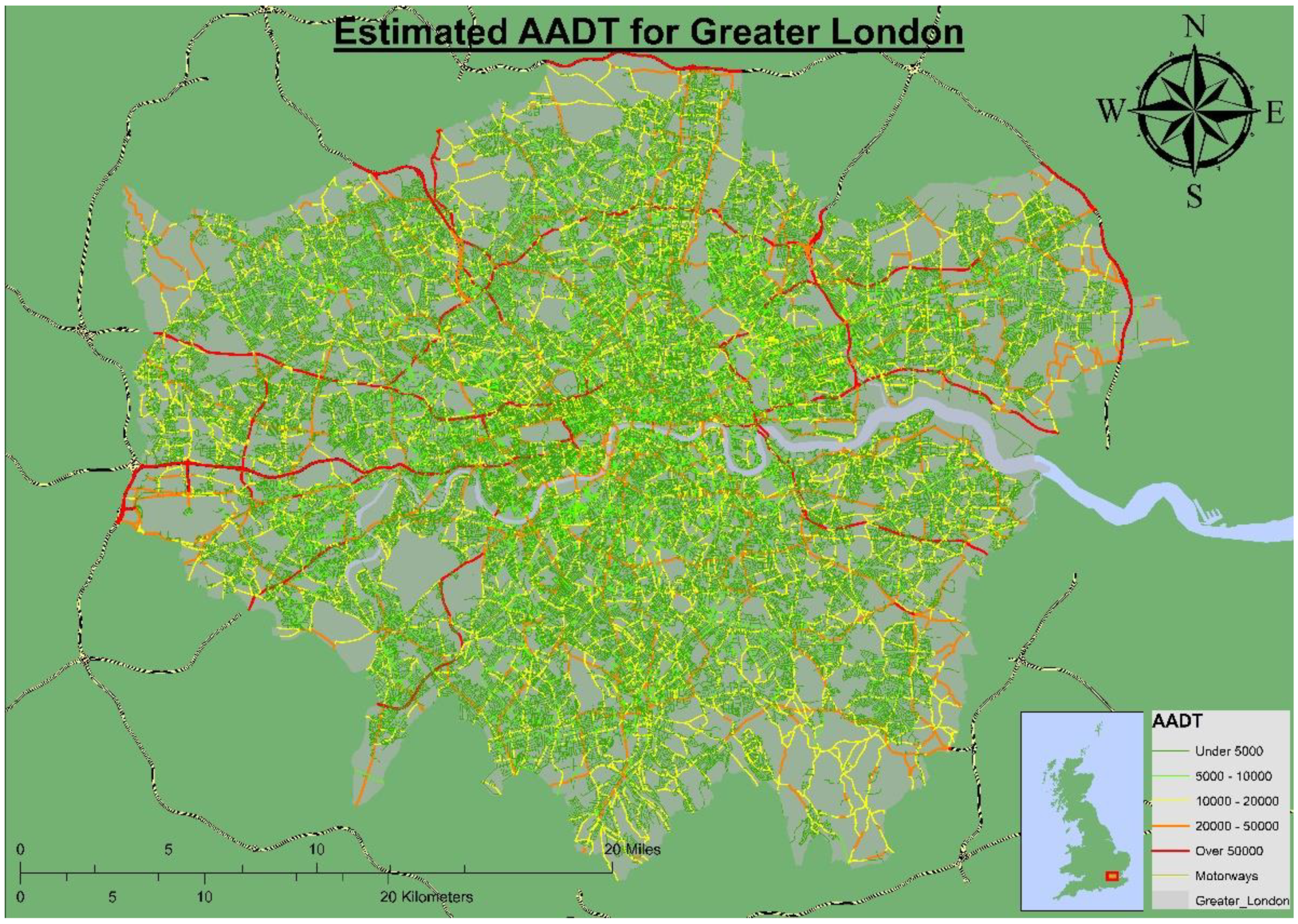
In Figure 2 the estimated AADT for all street segments in the Greater London area are presented, where roads with significantly higher traffic volumes can be distinguished. These are usually ‘A’ roads and parts of motorways. Roads around Heathrow airport, river crossings and major arteries also appear to carry heavy traffic loads, while secondary roads and streets in residential areas have lower AADT values.

The aggregated VKT estimations for all vehicle types and road classes are presented in

Table 2. Aggregate vehicle kilometres travelled (VKT) proportions by vehicle type and road class.

Vehicle Type	Road Class
	Motorways	A	B	C	U	All Roads
Cars	72.79%	77.37%	76.46%	81.65%	80.60%	78.62%
Buses 1	0.43%	2.46%	5.06%	2.19%	1.63%	2.28%
LGVs	15.91%	13.70%	13.11%	12.07%	12.98%	13.29%
HGVs	10.18%	3.78%	2.10%	2.84%	2.29%	3.61%
Two-wheeled	0.69%	2.69%	3.26%	1.26%	2.49%	2.21%
Total	6.76%	44.60%	6.4%	24.32%	17.91%	100%

¹ This vehicle type includes buses and coaches [65].

. One can observe that streets are mainly dominated by cars. Interesting also appears to be the high volume of HGVs on motorways as opposed to other road classes. By contrast, estimated bus traffic volumes are lowest on motorways.

Total average and annual estimated emissions for each vehicle type are presented in

Table 3. Daily average and total annual emissions by vehicle type (tonnes).

Vehicle Type	NOx	PM2.5	CO	CO2
Cars	23.93	0.38	24.62	14,810
Buses	9.50	0.10	2.70	0,181
LGVs	13.77	0.18	1.88	3,446
HGVs	7.66	0.09	2.35	3,038
Two-wheeled	0.28	0.02	8.74	0,250
Total—Average Daily	55.14	0.77	40.30	21,725
Total—Annual	20,126.10	281.05	14,709.50	7,929,625

. Annual emissions are estimated by multiplying average daily emissions by 365. Again, it is observed that highest emissions levels are originating from cars. Moreover, CO₂ emissions are similar for LGVs and HGVs although the number of HGVs and associated VKT are much lower compared to LGVs.

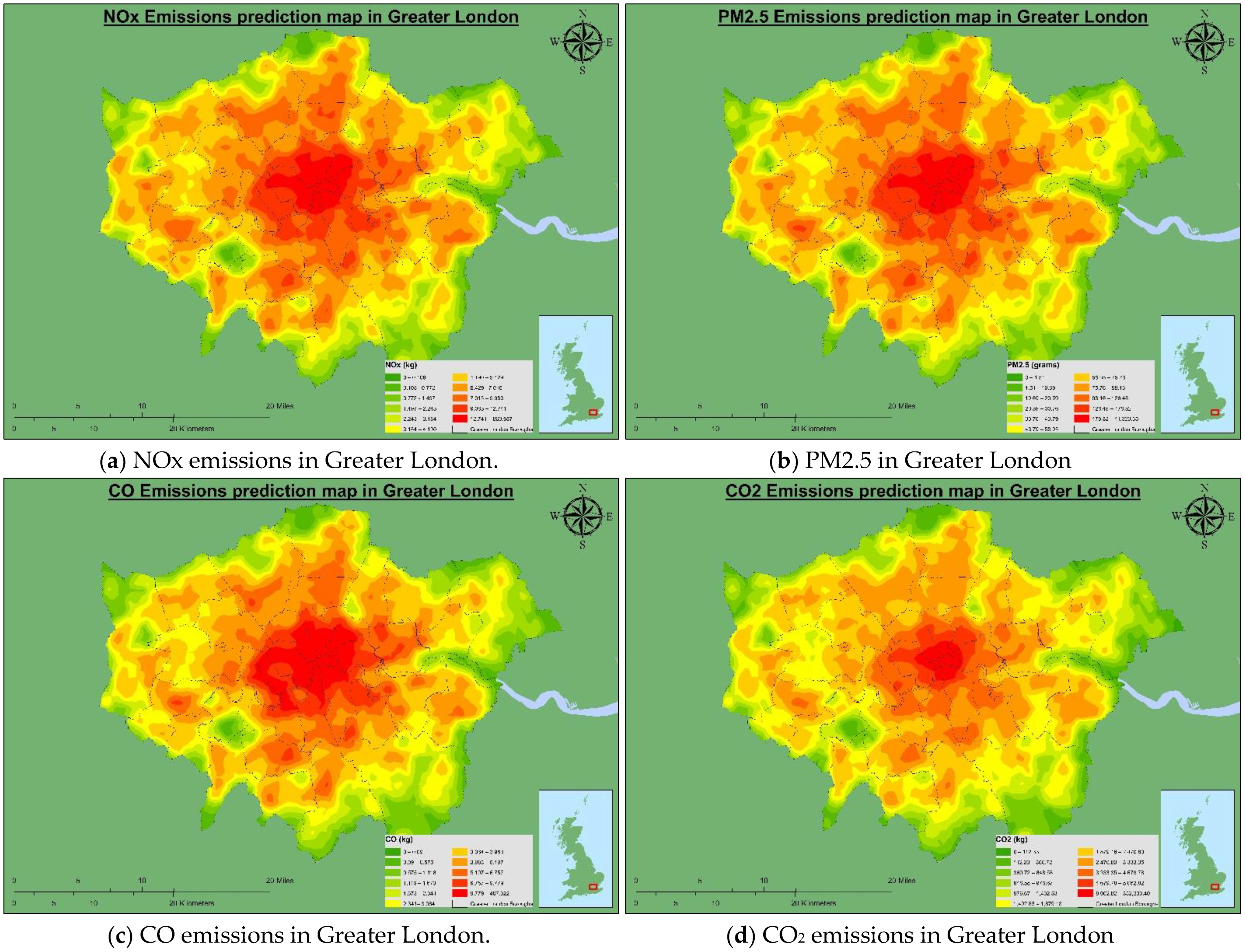
In Figure 3 emissions for the estimated pollutants and CO₂ are shown with London boroughs overlaid with heat maps for each pollutant and CO₂. Higher pollution can be observed in central and inner London as opposed to boroughs located far from the city centre. South London boroughs have lower level emissions compared to the north part of the city, reflecting the lower levels of traffic shown in Figure 2.

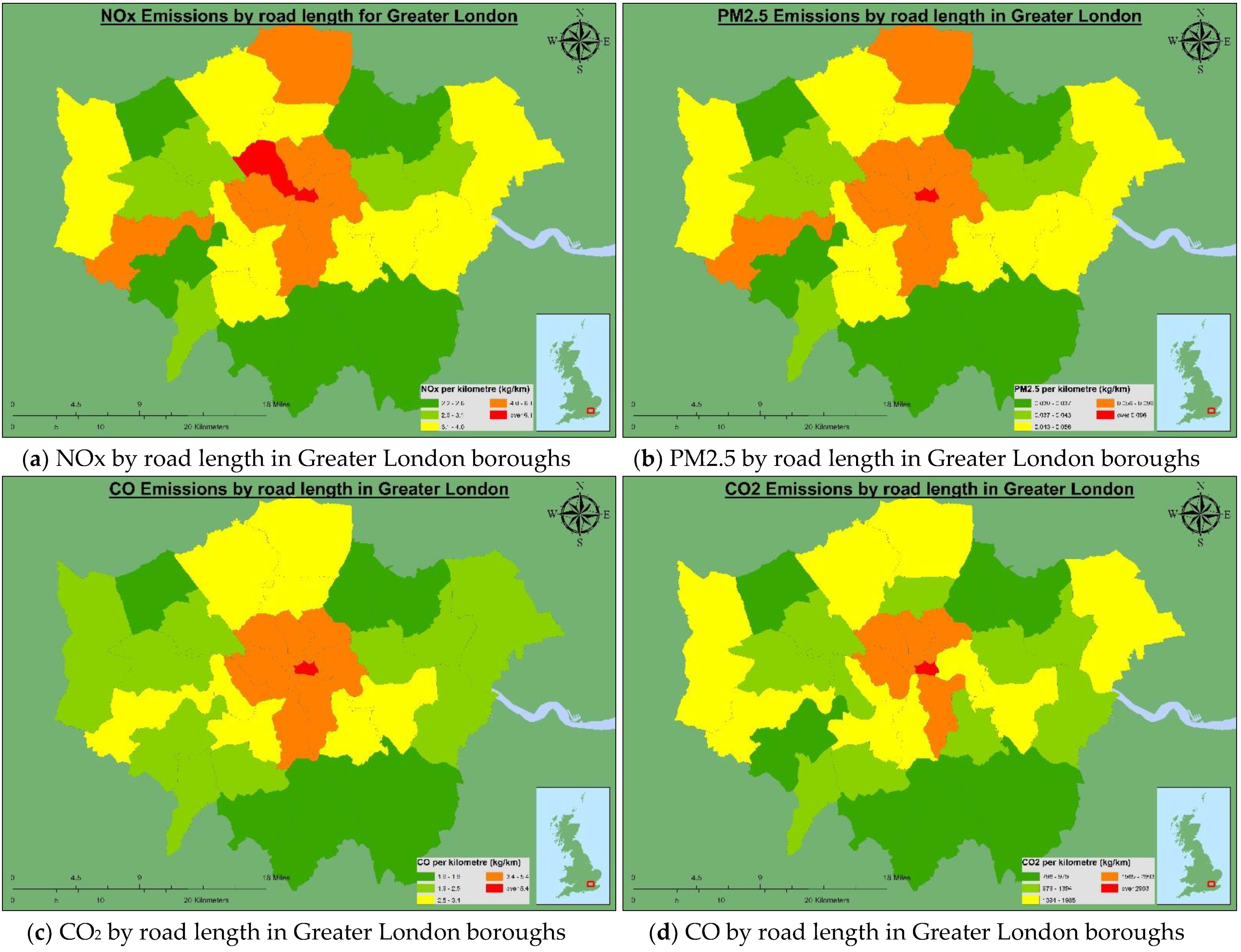
Similar patterns are observed in Figure 4 where emissions for each borough are mapped by the length of streets within the borough—kilograms of pollutant per kilometre of street length (kg/km). One can observe that some boroughs in the northern part of the city have higher values of emissions, particularly in the case of NO_x and PM_2.5.

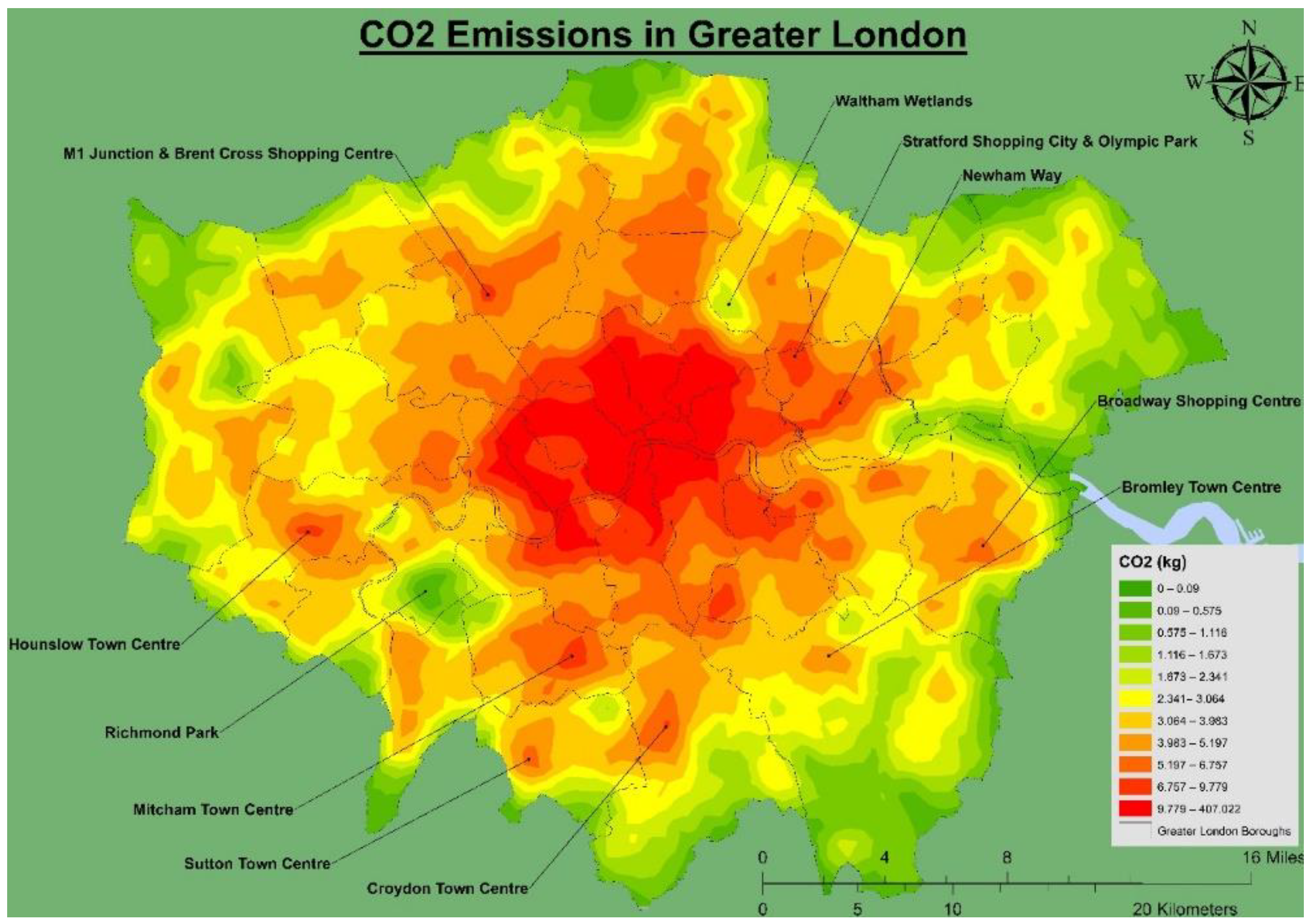
Interestingly, one can identify the impacts of large open spaces such as Richmond park indicated by green patches on the maps as well as the—negative—impacts of town centres and busy streets, indicated by smaller red patches around the city centre (Figure 5).

6. Discussion

The study focused on the emission estimation of NO_x PM_2.5, CO and CO₂ originating from road transport in the Greater London area. Estimation has been conducted for five road classes and five different vehicle types used by the Department for Transport (DfT) in the UK, by combining data from numerous sources and applying classification and regression modelling.

The results show higher levels of pollution in the city centre as expected, as can also be confirmed by similar studies in other urban areas [55,66]. For London in particular, our results can also be validated with those presented in [67] where PM_2.5 distribution is studied and higher levels of pollution are concentrated in central and inner London, as well as major road arteries. Estimated emissions from the method presented in this paper, are also comparable in most cases—with the exception of PM_2.5—with estimations from the London Atmospheric Emissions Inventory (LAEI) forming fraction of the NAEI for London [68]. The aggregated emissions are provided in

Table 4. Estimation comparison—tonnes/year.

	NOx	PM2.5	CO	CO2
LAEI	23,852.5	1,253.4	N/A	6,651,511
Authors’ Method	20,126.10	281.05	14,709.50	7,929,625

. The large deviation in estimations observed for PM_2.5 in Table 4 can be attributed to the methodology and factors taken into consideration when estimating emissions by NAEI. In the case of PM_2.5 emissions from breaks and tyres are also considered on top of the exhaust emissions.

Deviations in estimations from statistical approaches compared to standard emissions models are subject to various factors also reported in similar studies in Greater London and the UK as well as other countries, while significant deviations in estimations can be observed even among different emission models. For example, [29] compared COPERT and HBEFA to identify deviations in the estimations and concluded that both over-predicted PM emissions, with HBEFA results deviating more from actual measurements. In the case of NAEI, which is widely used in the UK, estimations have been usually found to deviate from other modelling approaches. For example, [69] indicate that NAEI tends to overestimate NO_x emissions, although it seems to underestimate volatile organic compounds [70]—not examined in our study. By contrast, [71] compare NO_x, PM₁₀ and CO₂ estimation with NAEI to find strong correlations, although in this study annual distance travelled is used and there is no differentiation between vehicle types.

However, over- and underestimations cannot be solely attributed to each modelling approach per se, but can be related to limitations in methodology and available data [8]. In our approach, one has also to consider modelling limitations, such as the classification and regression outcomes, the length of roads within the study area and the study area per se. First, from Table A2 one can observe that classification accuracy is significantly higher for ‘A’ roads, as opposed to other road classes, although accuracy for ‘U’ roads is relatively high as well (70%). Thus, an uncertainty in the classification of points and consequently in the estimation of AADT and VKT can result in biased emission estimations. However, from Table 2 one can see that VKT on ‘A’ roads and Motorways account for over 50% of total VKT. Including ‘U’ roads, the percentage is 68% indicating that for most modelled street segments, emissions are correctly estimated. Moreover, taking into account classification accuracy for ‘A’ roads as well as the fact that there is a large sample to train the algorithm for this road class and that AADT on motorways is directly counted—and not estimated with a model—we can also conclude that results for these two road types are more reliable as opposed to other road classes. Second, roads have been spatially clipped so as not to extend further than the Greater London boroughs and associated boundaries. That is, initial street segment lengths could be longer affecting estimation of VKT and related emissions. This can significantly affect estimations for motorways and attached outer London boroughs, where one can observe that even though these road types usually carry heavy traffic, VKT accounts for a smaller fraction of the total, due to the short length within the study area. Finally, the occurrence of satellite cities (i.e., smaller settlements around larger cities, separated from the metropolitan core by belts of rural territories [72,73]) attached to but outside Greater London can significantly affect emissions on the edges of the study area, an effect that cannot be captured in our study.

7. Conclusions and Future Work

Spatial distribution of AADT, VKT and associated emissions is of high importance for research in urban, transport as well as health and environmental planning. The methodology presented can provide a significant improvement in estimating emissions since all street segments of the study area are modelled, therefore delivering a better understanding of the spatial distribution of pollution levels in the area. Our approach can be used for both micro (e.g., street level) and macro (e.g., countries or states) analysis and consequently can be useful for both policy makers and planners. However, it is important to highlight that our method estimates and presents the spatial distribution of average daily emissions and not concentration of pollutants.

Based on the results presented here, additional research can follow. Firstly, the analysis can be extended to the Home Counties so as more accurate emissions in outer London can be estimated. Secondly, although we have tested three classification algorithms, other probabilistic classification models can be trialled to achieve higher classification accuracy and emission estimation if possible. Moreover, further subdivision of vehicle types based on the Euro standards (e.g., Pre-Euro, Euro 1, Euro 2, etc.) and related emission factors will allow to more detailed estimations. Finally, estimating pollutant concentrations associated with the estimated emissions, would allow further comparison of modelled and measured concentrations.

References

- Office for National Statistics. Road Transport and Air Emissions: Contribution of Road Transport to Greenhouse Gas and Air Pollutant Emissions; Office for National Statistics: Newport, UK, 2019.
- Latake, P.T.; Pawar, P. The Greenhouse Effect and Its Impacts on Environment. Int. J. Innov. Res. Creat. Technol. 2015, 1, 333–337. [Google Scholar]
- IPCC. Climate Change 2014 Synthesis Report; IPCC: Geneva, Switzerland, 2014. [Google Scholar]
- Department for Transport. Transport Energy and Environment Statistics 2011; Department for Transport: London, UK, 2018.
- DEFRA. Emissions of Air Pollutants in the UK, 1970 to 2016; DEFRA: London, UK, 2018.
- Ricardo Energy & Environment. Air Quality Damage Cost Update 2019; ED 59323; Ricardo Energy & Environment: Guildford, UK, 2019. [Google Scholar]
- European Environmental Agency. Costs of Air Pollution from European Industrial Facilities 2008–2012—An Updated Assessment; European Environmental Agency: Copenhagen, Denmark, 2014.
- Borge, R.; de Miguel, I.; de la Paz, D.; Lumbreras, J.; Pérez, J.; Rodríguez, E. Comparison of road traffic emission models in Madrid (Spain). Atmos. Environ. 2012, 62, 461–471. [Google Scholar] [CrossRef] [Green Version]
- Ong, H.C.; Mahlia, T.M.I.; Masjuki, H.H. A review on emissions and mitigation strategies for road transport in Malaysia. Renew. Sustain. Energy Rev. 2011, 15, 3516–3522. [Google Scholar] [CrossRef]
- Sookun, A.; Boojhawon, R.; Rughooputh, S.D.D.V. Assessing greenhouse gas and related air pollutant emissions from road traffic counts: A case study for Mauritius. Transp. Res. Part D Transp. Environ. 2014, 32, 35–47. [Google Scholar] [CrossRef]
- Tsagatakis, I.; Brace, S.; Passant, N.; Pearson, B.; Kiff, B.; Richardson, J.; Ruddy, M. UK Emission Mapping Methodology 2007; AEA Technology: Didcot, UK, 2017. [Google Scholar]
- Pang, Y.; Tsagatakis, I.; Murrells, T.; Brace, S. Methodology and Changes made in the 2014 NAEI Road Transport Inventory: A Briefing Note Produced for DECC on Changes in Fuel Consumption; Department for Business, Energy & Industrial Strategy: London, UK, 2016.
- Department for Transport. Road Lengths in Great Britain 2016. In 2016 the Total Road Length in Great Britain Was Estimated to Be 246,500 Miles, an Increase of 600 Miles (0.3 per cent) Compared to the Previous Year; Department for Transport: London, UK, 2019. [Google Scholar]
- McCord, M.R.; Yang, Y.; Jiang, Z.; Coifman, B.; Goel, P.K. Estimating Annual Average Daily Traffic from Satellite Imagery and Air Photos: Empirical Results. Transp. Res. Rec. 2003, 1855, 136–142. [Google Scholar] [CrossRef]
- Lowry, M. Spatial interpolation of traffic counts based on origin-destination centrality. J. Transp. Geogr. 2014, 36, 98–105. [Google Scholar] [CrossRef]
- Hankey, S.; Lu, T.; Mondschein, A.; Buehler, R. Spatial models of active travel in small communities: Merging the goals of traffic monitoring and direct-demand modeling. J. Transp. Health 2017, 7, 149–159. [Google Scholar] [CrossRef]
- Lu, T.; Buehler, R.; Mondschein, A.; Hankey, S. Designing a bicycle and pedestrian traffic monitoring program to estimate annual average daily traffic in a small rural college town. Transp. Res. Part D Transp. Environ. 2017, 53, 193–204. [Google Scholar] [CrossRef]
- Puliafito, S.E.; Allende, D.; Pinto, S.; Castesana, P. High resolution inventory of GHG emissions of the road transport sector in Argentina. Atmos. Environ. 2015, 101, 303–311. [Google Scholar] [CrossRef]
- Apronti, D.; Ksaibati, K.; Gerow, K.; Hepner, J.J. Estimating traffic volume on Wyoming low volume roads using linear and logistic regression methods. J. Traffic Transp. Eng. 2016, 3, 493–506. [Google Scholar] [CrossRef] [Green Version]
- Wang, T.; Gan, A.; Alluri, P. Estimating annual average daily traffic for local roads for highway safety analysis. Transp. Res. Rec. 2013, 5, 60–66. [Google Scholar] [CrossRef] [Green Version]
- Boulter, P.; McCrae, I.; Barlow, T. A Review of Instantaneous Emission Models for Road Vehicles; Transport Research Laboratory: Crowthorne, UK, 2007. [Google Scholar]
- Elkafoury, A.; Bady, M.; Aly, M.H.F.; Negm, A.M. Emissions Modeling for Road Transportation in Urban Areas: State-of-Art Review. In Proceedings of the 23rd International Conference on “Environmental Protection is a Must”, Alexandria, Egypt, 11–13 May 2013; pp. 1–16. [Google Scholar]
- De Blasiis, M.R.; Di Prete, M.; Guattari, C.; Veraldi, V.; Chiatti, G.; Palmieri, F. Investigating the influence of highway traffic flow condition on pollutant emissions using driving simulators. WIT Trans. Ecol. Environ. 2013, 174, 171–181. [Google Scholar] [CrossRef] [Green Version]
- Esteves-Booth, A.; Muneer, T.; Kubie, J.; Kirby, H. A review of vehicular emission models and driving cycles. Proc. Inst. Mech. Eng. Part C J. Mech. Eng. Sci. 2002, 216, 777–797. [Google Scholar] [CrossRef]
- Fallahshorshani, M.; André, M.; Bonhomme, C.; Seigneur, C. Coupling Traffic, Pollutant Emission, Air and Water Quality Models: Technical Review and Perspectives. Procedia Soc. Behav. Sci. 2012, 48, 1794–1804. [Google Scholar] [CrossRef]
- Smit, R.; Dia, H.; Morawska, L. Road Traffic Emission and Fuel Consumption Modelling: Trends, New Developments and Future Challenges; Nova Publishers: Hauppauge, NY, USA, 2009. [Google Scholar]
- Baškovic, K.; Knez, M. A Review of Vehicular Emission Models. Science 2013, 216, 3000. [Google Scholar]
- Wyatt, D.W. Assessing Micro Scale Carbon Dioxide (CO2) Emission on UK Road Networks using a Coupled Traffic Simulation and Vehicle Emission Model. Ph.D. Thesis, University of Leeds, Leeds, UK, 2017. [Google Scholar]
- Fontaras, G.; Franco, V.; Dilara, P.; Martini, G.; Manfredi, U. Development and review of Euro 5 passenger car emission factors based on experimental results over various driving cycles. Sci. Total Environ. 2014, 468–469, 1034–1042. [Google Scholar] [CrossRef]
- Elkafoury, A.; Negm, A.; Aly, M.; Bady, M.; Ichimura, T. Develop dynamic model for predicting traffic CO emissions in urban areas. Environ. Sci. Pollut. Res. 2016, 23, 15899–15910. [Google Scholar] [CrossRef]
- Boulter, P.G.; McCrae, I.S. ARTEMIS: Assessment and Reliability of Transport Emission Models and Inventory Systems—Final Report; TRL: Crowthorne, UK, 2007; 350p. [Google Scholar]
- Wang, H.; McGlinchy, I. Review of vehicle emission modelling and the issues for New Zealand. In Proceedings of the 32nd Australasian Transport Research Forum (ATRF), Auckland, New Zealand, 29 September–1 October 2009; pp. 1–13. [Google Scholar]
- Joumard, R.; André, J.-M.; Rapone, M.; Zallinger, M.; Kljun, N.; André, M.; Samaras, Z.; Roujol, S.; Laurikko, J.; Weilenmann, M.; et al. Emission Factor Modelling for Light Vehicles within the European Artemis Model. In Proceedings of the 16th International Symposium Transport and Air Pollution, Graz, Austria, 16–17 June 2008; pp. 1–10. [Google Scholar]
- Martinet, S.; Liu, Y.; Louis, C.; Tassel, P.; Perret, P.; Chaumond, A.; Andre, M. Euro 6 Unregulated Pollutant Characterization and Statistical Analysis of After-Treatment Device and Driving-Condition Impact on Recent Passenger-Car Emissions. Environ. Sci. Technol. 2017, 51, 5847–5855. [Google Scholar] [CrossRef] [Green Version]
- Iodice, P.; Senatore, A. Analytical-experimental analysis of last generation medium-size motorcycles emission behaviour under real urban conditions. Int. J. Automot. Mech. Eng. 2015, 12, 3018–3032. [Google Scholar] [CrossRef]
- Liu, C.; Susilo, Y.O.; Karlström, A. Estimating changes in transport CO2 emissions due to changes in weather and climate in Sweden. Transp. Res. Part D Transp. Environ. 2016, 49, 172–187. [Google Scholar] [CrossRef]
- Hausberger, S.; Rexeis, M.; Zallinger, M.; Luz, R. Emission Factors from the Model PHEM for the HBEFA Version 3; Report Nr. I-20/2009 Haus-Em 33/08/679 from 07.12.2009; Graz University of Technology: Graz, Austria, 2009. [Google Scholar]
- Ntziachristos, L.; Gkatzoflias, D.; Kouridis, C. Information Technologies in Environmental Engineering; Springer: Berlin/Heidelberg, Germany, 2009. [Google Scholar] [CrossRef]
- Vanhulsel, M.; Degraeuwe, B.; Beckx, C.; Vankerkom, J.; De Vlieger, I. Road transportation emission inventories and projections—Case study of Belgium: Methodology and pitfalls. Transp. Res. Part D Transp. Environ. 2014, 27, 41–45. [Google Scholar] [CrossRef]
- Wang, H.; Fu, L.; Bi, J. CO2 and pollutant emissions from passenger cars in China. Energy Policy 2011, 39, 3005–3011. [Google Scholar] [CrossRef]
- Mascia, M.; Hu, S.; Han, K.; North, R.; Van Poppel, M.; Theunis, J.; Beckx, C.; Litzenberger, M. Impact of Traffic Management on Black Carbon Emissions: A Microsimulation Study. Netw. Spat. Econ. 2017, 17, 269–291. [Google Scholar] [CrossRef] [Green Version]
- Brand, C. Transport Carbon Model Reference Guide 2010; UK Energy Research Centre: London, UK, 2010. [Google Scholar]
- Oxley, T.; Valiantis, M.; Elshkaki, A.; ApSimon, H.M. Background, Road and Urban Transport modelling of Air quality Limit values (The BRUTAL model). Environ. Model. Softw. 2009, 24, 1036–1050. [Google Scholar] [CrossRef]
- ApSimon, H.M.; Warren, R.F.; Wilson, J.J.N. The abatement strategies assessment model-ASAM: Applications to reductions of sulphur dioxide emissions across Europe. Atmos. Environ. 1994, 28, 649–663. [Google Scholar] [CrossRef]
- Oxley, T.; ApSimon, H.; Dore, A.; Sutton, M.; Hall, J.; Heywood, E.; Gonzales del Campo, T.; Warren, R. The UK Integrated Assessment Model, UKIAM: A National Scale Approach to the Analysis of Strategies for Abatement of Atmospheric Pollutants under the Convention on Long-Range Transboundary Air Pollution. Integr. Assess. 2003, 4, 236–249. [Google Scholar] [CrossRef]
- Degraeuwe, B.; Pisoni, E.; Christidis, P.; Christodoulou, A.; Thunis, P. SHERPA-city: A web application to assess the impact of traffic measures on NO2 pollution in cities. Environ. Model. Softw. 2021, 135, 104904. [Google Scholar] [CrossRef]
- Brown, P.; Wakeling, D.; Pang, Y.; Murrells, T. Methodology for the UK’s Road Transport Emissions Inventory: Version for the 2016 National Atmospheric Emissions Inventory; Department for Business, Energy & Industrial Strategy: London, UK, 2018.
- Ren, W.; Xue, B.; Geng, Y.; Lu, C.; Zhang, Y.; Zhang, L.; Fujita, T.; Hao, H. Inter-city passenger transport in larger urban agglomeration area: Emissions and health impacts. J. Clean. Prod. 2016, 114, 412–419. [Google Scholar] [CrossRef]
- Zheng, Y.; Weng, Q. Evaluation of the correlation between remotely sensing-based and GIS-based anthropogenic heat discharge in Los Angeles County, USA. In Proceedings of the 4th International Workshop on Earth Observation and Remote Sensing Applications (EORSA), Guangzhou, China, 4–6 July 2016; pp. 324–328. [Google Scholar] [CrossRef]
- Leduc, G. Road Traffic Data: Collection Methods and Applications; EUR Number Tech Note JRC 47967; European Commission: Brussels, Belgium, 2008; 55p. [Google Scholar]
- Setyawan, A.; Kusdiantoro, I. The effect of pavement condition on vehicle speeds and motor vehicles emissions. Procedia Eng. 2015, 125, 424–430. [Google Scholar] [CrossRef] [Green Version]
- Jung, S.; Kim, J.; Kim, J.; Hong, D.; Park, D. An estimation of vehicle kilometer traveled and on-road emissions using the traffic volume and travel speed on road links in Incheon City. J. Environ. Sci. 2017, 54, 90–100. [Google Scholar] [CrossRef]
- Labib, S.M.; Neema, M.N.; Rahaman, Z.; Patwary, S.H.; Shakil, S.H. Carbon dioxide emission and bio-capacity indexing for transportation activities: A methodological development in determining the sustainability of vehicular transportation systems. J. Environ. Manag. 2018, 223, 57–73. [Google Scholar] [CrossRef] [PubMed] [Green Version]
- Patarasuk, R.; Gurney, K.R.; O’Keeffe, D.; Song, Y.; Huang, J.; Rao, P.; Buchert, M.; Lin, J.C.; Mendoza, D.; Ehleringer, J.R. Urban high-resolution fossil fuel CO2 emissions quantification and exploration of emission drivers for potential policy applications. Urban Ecosyst. 2016, 19, 1013–1039. [Google Scholar] [CrossRef]
- Fu, M.; Kelly, J.A.; Clinch, J.P. Estimating annual average daily traffic and transport emissions for a national road network: A bottom-up methodology for both nationally-aggregated and spatially-disaggregated results. J. Transp. Geogr. 2017, 58, 186–195. [Google Scholar] [CrossRef]
- Sfyridis, A.; Agnolucci, P. Annual average daily traffic estimation in England and Wales: An application of clustering and regression modelling. J. Transp. Geogr. 2020, 83, 102658. [Google Scholar] [CrossRef]
- Ajtay, D.; Weilenmann, M. Compensation of the exhaust gas transport dynamics for accurate instantaneous emission measurements. Environ. Sci. Technol. 2004, 38, 5141–5148. [Google Scholar] [CrossRef]
- Zhou, X.; Tanvir, S.; Lei, H.; Taylor, J.; Liu, B.; Rouphail, N.M.; Frey, H.C. Integrating a simplified emission estimation model and mesoscopic dynamic traffic simulator to efficiently evaluate emission impacts of traffic management strategies. Transp. Res. Part D Transp. Environ. 2015, 37, 123–136. [Google Scholar] [CrossRef]
- Sturm, P.J.; Kirchweger, G.; Hausberger, S.; Almbauer, R.A. Instantaneous emission data and their use in estimating road traffic emissions. Int. J. Veh. Des. 1998, 20, 181–191. [Google Scholar] [CrossRef]
- Friedman, J.H. Greefy Function Approximation: A Gradient Boosting Machine. Ann. Stat. 2001, 29, 1189–1232. [Google Scholar] [CrossRef]
- Brown, I.; Mues, C. An experimental comparison of classification algorithms for imbalanced credit scoring data sets. Expert Syst. Appl. 2012, 39, 3446–3453. [Google Scholar] [CrossRef] [Green Version]
- Rawi, R.; Mall, R.; Kunji, K.; Shen, C.H.; Kwong, P.D.; Chuang, G.Y. PaRSnIP: Sequence-based protein solubility prediction using gradient boosting machine. Bioinformatics 2017, 34, 1092–1098. [Google Scholar] [CrossRef] [Green Version]
- Breiman, L. Bagging predictors. Mach. Learn. 1996, 24, 123–140. [Google Scholar] [CrossRef] [Green Version]
- Breiman, L. Random Forests. Mach. Learn. 2001, 45, 5–32. [Google Scholar] [CrossRef] [Green Version]
- Department for Transport. Road Traffic Estimates; Department for Transport: London, UK, 2014.
- Munir, S.; Mayfield, M.; Coca, D.; Mihaylova, L.S. A nonlinear land use regression approach for modelling NO2 concentrations in urban areas—Using data from low-cost sensors and diffusion tubes. Atmosphere 2020, 11, 736. [Google Scholar] [CrossRef]
- Fecht, D.; Hansell, A.L.; Morley, D.; Dajnak, D.; Vienneau, D.; Beevers, S.; Toledano, M.B.; Kelly, F.J.; Anderson, H.R.; Gulliver, J. Spatial and temporal associations of road traffic noise and air pollution in London: Implications for epidemiological studies. Environ. Int. 2016, 88, 235–242. [Google Scholar] [CrossRef] [PubMed] [Green Version]
- LAEI. London Atmospheric Emissions Inventory (LAEI) 2013 Methodology; London Atmospheric Emissions Inventory (LAEI): London, UK, 2013.
- Vaughan, A.R.; Lee, J.D.; Misztal, P.K.; Metzger, S.; Shaw, M.D.; Lewis, A.C.; Purvis, R.M.; Carslaw, D.C.; Goldstein, A.H.; Hewitt, C.N.; et al. Spatially resolved flux measurements of NOX from London suggest significantly higher emissions than predicted by inventories. Faraday Discuss. 2016, 189, 455–472. [Google Scholar] [CrossRef] [PubMed] [Green Version]
- Valach, A.C.; Langford, B.; Nemitz, E.; Mackenzie, A.R.; Hewitt, C.N. Seasonal and diurnal trends in concentrations and fluxes of volatile organic compounds in central London. Atmos. Chem. Phys. 2015, 15, 7777–7796. [Google Scholar] [CrossRef] [Green Version]
- Chatterton, T.; Barnes, J.; Wilson, R.E.; Anable, J.; Cairns, S. Use of a novel dataset to explore spatial and social variations in car type, size, usage and emissions. Transp. Res. Part D Transp. Environ. 2015, 39, 151–164. [Google Scholar] [CrossRef] [Green Version]
- Sorensen, A. Subcentres and satellite cities: Tokyo’s 20th century experience of planned polycentrism. Int. Plan. Stud. 2001, 6, 9–32. [Google Scholar] [CrossRef] [Green Version]
- Bontje, M. Shenzhen: Satellite city or city of satellites? Int. Plan. Stud. 2019, 24, 255–271. [Google Scholar] [CrossRef] [Green Version]
- Pointer, G. The UK’s major urban areas. In Focus on People and Migration; Chappell, R., Ed.; Palgrave Macmillan: London, UK, 2005; pp. 45–60. [Google Scholar]
Figure 1.
London vehicle fleet composition (LGV—Light Goods Vehicle, HGV—Heavy Goods Vehicle, Artic—Articulated Vehicle, TfL—Transport for London).
Figure 2.
Annual average daily traffic (AADT) by street segment in Greater London.
Figure 3.
Air pollutants and CO2 estimation heat maps.
Figure 4.
Air Pollutants and CO2 emissions in kilograms per street kilometre (kg/km) for London boroughs.
Figure 5.
Open spaces and town centre’s impact on CO2 emissions.