Article

The ESTE Decision Support System for Nuclear and Radiological Emergencies: Atmospheric Dispersion Models

ABmerit, s.r.o., Hornopotočná 1, P.O. Box 200, 917 01 Trnava, Slovakia
*
Author to whom correspondence should be addressed.
Submission received: 17 December 2020 / Revised: 25 January 2021 / Accepted: 26 January 2021 / Published: 3 February 2021

Abstract

:
The ESTE system is running in nuclear crisis centers at various levels of emergency preparedness and response in Slovakia, the Czech Republic, Austria, Bulgaria, and Iran (at the Bushehr Nuclear Power Plant, monitored by the International Atomic Energy Agency (IAEA)). ESTE is a decision-support system that runs 24/7 and serves the crisis staff to propose actions to protect inhabitants against radiation in case of a nuclear accident. ESTE is also applicable as a decision-support system in case of a malicious act with a radioactive dispersal device in an urban or industrial environment. The dispersion models implemented in ESTE are the Lagrangian particle model (LPM) and the Puff trajectory model (PTM). We describe model approaches as implemented in ESTE. The PTM is applied in ESTE for the dispersion calculation near the point of release, up to 100 km from the point of a nuclear accident. The LPM for general atmospheric transport is applied for short-range, meso-scale and large-scale dispersion, up to dispersion on the global scale. Additionally, a specific micro-scale implementation of the LPM is applied for urban scale dispersion modeling. The dispersion models of ESTE are joined with radiological-consequences models to calculate a complete spectrum of radiological parameters—effective doses, committed doses, and dose rates by various irradiation pathways and by various radionuclides. Finally, radiation protective measures, like sheltering, iodine prophylaxis, or evacuation, evaluated on the base of predicted radiological impacts, are proposed. The dispersion and radiological models of the state-of-the-art ESTE systems are described. The results of specific analyses, like the number of particles applied, the initial spatial distribution of the source, and the height of the bottom reference layer, are presented and discussed.

Graphical Abstract

1. Introduction

The key elements of decision-support systems (DSSs) for emergency preparedness and response in case of nuclear and radiological emergencies are assessment of the level of threat to the population due to the predicted or already released radioactivity to the environment, and recommendations of actions to secure the health of the inhabitants in the first place. Toward these aims, a DSS performs a radiological impact calculation, consisting of a calculation of atmospheric transport and dispersion of the radioactive material, and consequently of dose-prognosis evaluation. The dose calculation results in the recommended actions, which primarily are sheltering, iodine prophylaxis, and evacuation, and secondarily, actions in agriculture.
These are the basic features of the ESTE nuclear decision-support system, the approaches and solutions of which to atmospheric dispersion and radiological dose evaluation, are described and compared. Besides these features, the ESTE system is a complex decision-support system for nuclear emergencies.
First of all, the ESTE system is capable of performing an assessment of an accidental source term based on characteristics and conditions of the nuclear power plant in an emergency situation [1]. The basic assessment process in determination of the predicted accidental source term follows the approach of [2,3,4,5]. The assessment includes an evaluation of the state of the reactor core or the state of the fuel in the spent fuel pool, and identification of potential pathways to the atmosphere in the environment, with an evaluation of the state of the barriers (like containment tightness). In implementations specific to one particular nuclear power plant, all these analyses could be provided even in automatic mode by connection to and subsequent evaluation of online technological and radiation measurements of the nuclear power plant. To that purpose, in such implementations, plant-specific algorithms are implemented in the evaluation modules. Alternatively, the evaluated states of the nuclear power plant systems can be inserted by the operator of the system as well. The accidental source term assessment capabilities of ESTE were benchmarked in [6], in a comparison with other nuclear emergency source term evaluation tools and methods.
In all cases, a precalculated database of core inventories and inventories of spent fuel pools is integral element of the system. The inventories are calculated by the software SCALE [7], based on direct plant-specific data or data of [8].
The most important feature and unique approach of the nuclear DSS ESTE is in connection with modules for assessment of accidental release of harmful radionuclides, with the state-of-the-art dispersion models and radiological-impact models.
The calculated ensemble of radiological parameters considered in ESTE are dose rates, doses by external irradiation from radionuclides in atmosphere, doses by external irradiation from radionuclides deposited on terrain, doses by inhalation of airborne radionuclides, and doses by ingestion of contaminated foodstuffs.
The evaluation of impacts on population and recommendation of protective measures is supported by an implemented geographical information system and a database of population. Thus, the proposed measures are improved by the number of affected inhabitants with their age structures, for example.
The ESTE system is used for real-time response to accidents at nuclear installations, and that fact determines the features of the implemented transport and dispersion models. The system is running in the nuclear crisis centers of Slovakia, the Czech Republic, Austria, Bulgaria, and Iran, either directly on the national level or on the level of the nuclear facility, but still with a close connection to the national level (in Iran, it is the crisis center of the nuclear power plant Bushehr, a facility monitored and inspected by the IAEA).
The models implemented in the ESTE system—application of the Puff trajectory model (PTM) and Lagrangian particle models (LPM) are demonstrated and discussed here. The Lagrangian particle model is introduced in two alternative ways—one implementation covers the dispersion calculation on meso- and long-scales, while the other covers the micro-scale on the level of dispersion in urban environment. The LPM for real-time long-range calculation is based on the methods of parallel computing and utilization of a graphical card (CUDA technology). Emphasis is given to the description and comparison of the applied atmospheric dispersion models. Results of case studies and of the dispersion calculation after the Fukushima accident are demonstrated.
The urban-oriented LPM is applicable either: (i) in case of a malicious act, with application of a radiological dispersion device (RDD) or dirty bomb in an urban environment, or (ii) in industrial accidents. In both, the system performs an evaluation of the situation in close vicinity to the event.

2. Atmospheric Dispersion Models in ESTE

2.1. Lagrangian Particle Model: Specific Set-Up Assumptions in ESTE

The LPM uses a large number of independent particles to describe the diffusion of radionuclides in the atmosphere, and it performs a simulation of the movement and dispersion of particles inside the wind field. Each particle carries a specific amount of radionuclides from the radioactive cloud. In general, the wind field consists of a mean wind field and a turbulent field. The basic equations for the particle positions are:
xi (t + ∆t) = xi(t) + Ui.∆t + ui.∆t
where xi as the i-th component of (x1,x2,x3) specifies the position of the particle (at the times t and t + Δt), ∆t is the time step, Ui as the i-th component of (U1,U2,U3) is the velocity vector of the mean wind field at the given position (x,y,z), and (u1,u2,u3) is the turbulent component of velocity vector. The mean wind field is included in the provided numerical weather-prediction data (NWP data) directly. The LPM model of the ESTE system requires NWP data for its run. The model is able to apply various sources of NWP data; for example, data from the European Centre for Medium-Range Weather Forecasts (ECMWF), or data from the National Weather Service of the National Oceanic and Atmospheric Administration, USA (NWS/NOAA). The turbulent component of velocity vector is expressed using Langevin equation [9].
dui = ai(x,u,t) dt + bij(x,u,t)dWj
where a is the drift term and b is the diffusion term. Both of them are a function of particle position and turbulent velocity. dWj is incremental components of a Wiener process, here a Gaussian random variable. The LPM implemented in ESTE is based on a theoretical description of the FLEXPART model [10], and therefore both drift and diffusion terms obtain the form as in the FLEXPART model [10].
The implementation in ESTE was validated successfully several times in various projects, e.g., a comparison in [11] was performed directly with the FLEXPART model implemented in TAMOS (the Austrian emergency response modeling system).
Moreover, the implemented LPM model in the ESTE system enabled the simulation of impacts of the Fukushima accident, even at transcontinental distances. Here, we focus only on the simple comparison of the transport time (a further comparison was not performed due to its complexity). In the Supplementary Materials, in which a visualization in the form of video of the performed simulation is included (video S3), the impacts on Europe, especially on central Europe, were the center of interest. The simulation shows modeled atmospheric dispersion in the northern hemisphere of the released I-131 (equal to 1.5 × 10¹⁷ Bq as estimated by ESTE, based on a reverse estimation from the dose rate measured in the area of the nuclear power plant (NPP), and on assumption of partial core damage or partial melting in SFP [12]). The release was modeled from March 12 to 14, 2011. The results of dispersion and radiological impacts are visualized in subsequent days, from March 15 to March 30, 2011. The control forecast of the operational archive of the ECMFW data was applied. A basic estimate resulting from the simulation is that the airborne contamination would reach the central Europe approximately on March 24, 2011. For a comparison, the first reported measurement of I-131 in the Czech Republic was on March 23 [13], which represents an acceptable result.
Specific aspects of the LPM of ESTE that have influence on dispersion and radiation impacts calculation are:
Dry deposition—characterized by deposition velocity νd (in m.s−1), which is specified for various types of airborne material (e.g., gases, aerosols, iodine forms) and ground features (e.g., urban, forest, water). Deposited material in time step Δt is then calculated as:
Δm = m (1 − exp(−νd Δt/h))
where m is the amount of activity born by particles in the lowest reference layer with the height h.
Wet deposition—following the model in [14], this is governed in the LPM of ESTE (and in the implemented PTM as well) by the washout coefficient Λ, which depends on the precipitation rate I (in mm/h):
Λ = cwo I.
cwo is the coefficient of wet deposition, and is set to cwo = 1.3 × 10⁻⁴ s−1 for elemental iodine, cwo = 1.3 ×10⁻⁶ s−1 for organic iodine, and cwo = 2.6 × 10⁻⁵ s−1 for all radionuclides in aerosol form. The deposited material in time step Δt is assumed to follow the formula:
Δm = m (1 − exp(−Λ Δt))
where the approach applied in ESTE assumes the washout along the whole height of the atmospheric boundary layer (ABL), and the height of the clouds is not taken into account.
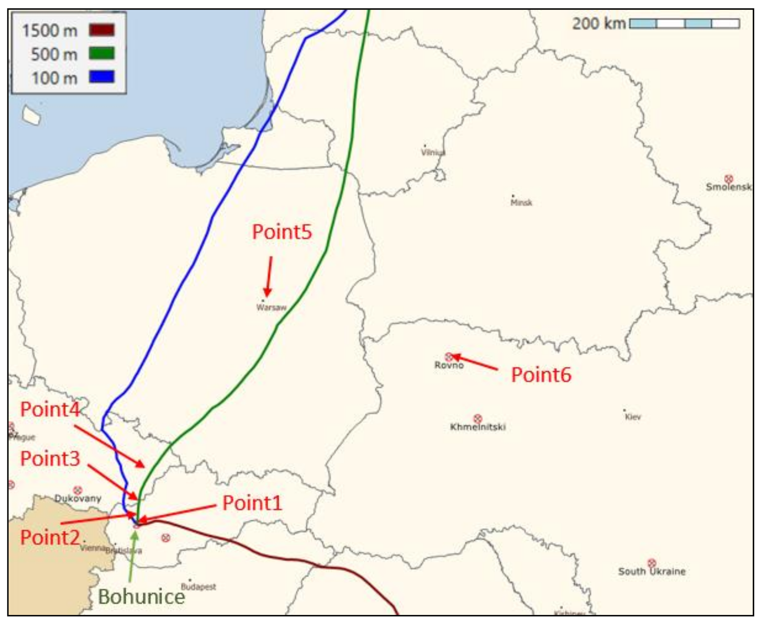
Release points—the position of the leakage point affects the impacts in the vicinity of nuclear facility in which the accident took place, but the leakage point in a real nuclear disaster can be uncertain and unknown. Generally, the leakage of harmful radionuclides can occur in any part of the containment structure in case of containment leakage, in the outlet of the plant ventilation stack, or in the outlet of the containment ventilation system. Moreover, the inner conditions inside the nuclear facility, like overpressure, fire, and explosions, can considerably affect the leakage conditions. The initial spatial distribution of the release points in the LPM of the ESTE system can be set up as a point source at a given height, a line-shape source, a source in the shape of a cylinder, or a hemisphere. In ESTE systems running in nuclear crisis centers, an assumption of a vertical-line-shaped source is applied, with the line center at the height of the realized release pathways. The center might be located at the height of the containment building, or at the height of the roof of the machinery room, at the height of the outlet of the reactor building ventilation stack, or at the outlet of the containment annulus ventilation. The performed study of the influence of initial spatial distribution of the release points at the beginning of the dispersion calculation is presented and discussed in Section 3.2.
Height of the bottom reference layer of air—this is the air layer that is used to evaluate the air concentration over the ground surface, applied in dry-deposition calculations, as well as in impact calculations (especially for effective dose by inhalation). As the previous aspect of the simulation setup, the modeled bottom-air-layer height above ground also affects the calculated impacts in the vicinity of the nuclear facility in which the accident took place. In the LPM of the ESTE system, the height of the bottom layer of air is set to 100 m. The results of our study of the influence of the height of the bottom reference layer of air are presented and discussed in Section 3.3.
Total number of modeled particles—the accuracy of dispersion calculation and radiological impacts calculation is determined by the total number of modeled particles. A relatively high number of particles is expected for the calculation in order to achieve an acceptable level of accuracy. The higher the number of particles, the longer the time to carry out the calculations. The time is strictly controlled in decision-support systems like ESTE that are in real operation in nuclear crisis centers. An acceptable time to carry out the calculations in local scale and mesoscale is about 15 min. In the case of ESTE, the parameters affecting the duration of impact calculation, to which the number of particles belongs, are set to fulfill this time limit. Naturally, if the calculations are performed at a large or global scale where the modeled phenomenon is on the level of several days or weeks (for example, modeling of the atmospheric transport and impacts of the Fukushima accident to central Europe), then the time limit for duration of the calculation is less strict, allowing a longer calculation and a higher number of modeled particles. Our study of the influence of the total number of modeled particles is presented and discussed in Section 3.1.
Number of radionuclides in the source term—the nuclear reactor core inventory consists of more than 1000 various isotopes created as a result of nuclear fission. At the same time, many of them are short-lived isotopes or isotopes with a negligible radiological impact. In case of a nuclear disaster, about 50 isotopes have the potential to be released into the environment in a significant amount, and also to cause a significant threat to humans and the environment. This group is covered by the set of radionuclides (Table 1) assumed at the input, in all modeled processes of the LPM in ESTE, as well as in radiological models of ESTE.
calculation of radiological parameters includes evaluation of the following quantities:
Committed effective dose by inhalation: the instant dose rate DRinhal and the integral dose Dinhal are calculated as:
DRinhal (n) = C0 (n) CFinhal (age,n) BR(age)
Dinhal (n) = Cint (n) CFinhal (age,n) BR(age)
where C0 is the actual air concentration, Cint is the time-integrated concentration in the bottom reference layer for radionuclide n, BR is the breathing rate, depending on the age category, and CFinhal is the conversion factor for the committed effective dose for inhalation, depending on the age and nuclide.
External dose by deposition: the instant dose rate is calculated as:
DRdepo (n) = D0 (n) CFdepo (n)
where D0 (n) is the deposition of radionuclide n on the terrain, CFdepo is the conversion factor for the external dose via deposition, as a function of radionuclide.
External dose by cloudshine: the instant dose rate is calculated as:
DRcloud (n) = C0 (n) CFcloud (n)
where C0(n) is the air concentration in the bottom reference layer, and CFcloud is the conversion factor for cloudshine, and dependent on the radionuclide. The factors represent an approach of semi-infinite cloud of constant concentration, i.e., the point of interest, either a radiation monitor or a human, is immersed in the activity of the air hemisphere with constant concentration.

2.2. Puff Trajectory Model

The Puff trajectory model (PTM) implemented in ESTE is a puff transport model combined with a Gaussian dispersion model in the horizontal direction and with a model based on a diffusion equation in the vertical direction. The release consists of puffs, and each puff carries a particular amount of the released radionuclides, which is the released activity per a specific time period, e.g., in units [Bq/1 h] or [Bq/10 min].
Basic model components and assumptions of the implemented PTM are:
Advection: The trajectories of the puffs are obtained as integrated paths for the wind field of numerical weather prediction data:
x(t + ∆t) = x(t) + U.∆t, y(t + ∆t) = y(t) + V.∆t
where U, V represent horizontal components of the wind field, and x and y are the characterized position of the puff in the given times t and t + ∆t. Both components U and V are dependent on height, and the height is taken as the height of center of mass of the puff.
Vertical dispersion: The puffs are distributed in many vertical layers, and the carried activity is mixing among these layers. In the ESTE system, the model works with the assumption of a division of the atmosphere into 10 equally thick layers. Diffusion coefficients are characterized using formulas [14]. In that applied approach, they are functions of the Pasquill category of stability and functions of the height above the terrain. The assumed height of the atmosphere, here meaning air between the ground and the atmospheric boundary layer (ABL), is related to the Pasquill category of stability (see [14]). In cases of very unstable conditions (i.e., category A) and very stable conditions (i.e., category F), which represent two extreme situations, the height of ABL is 1600 m and 200 m above the ground, respectively.
Horizontal dispersion: This is represented by a Gaussian model, where the puff sigma functions depend on wind speed, category stability, and travel distance. The included sigma functions [15] are dealing with rural and urban environments, as well as calm conditions (applying Briggs and Gifford formulas). The applied Briggs formulas are listed in Table 2.
Further assumptions and details of the implemented PTM are described in [1].
The assumed layer approach for vertical diffusion defines only mean, evenly distributed concentrations within the given layer. The bottom air layer is the reference layer for the calculation of air concentration, applied in the calculation of deposition and radiological parameters.
The height of the release, together with timing and nuclide composition of the release, are the attributes of the source term. The release height specifies one of the calculation layers in which the release point is situated and in which we assume an even distribution of released radioactive material. Releases as a function of time are realized as series of puffs, where each puff carries the specific amount of the leaked activity corresponding to a specific time interval of the release. Time intervals that express the course of the leak in time are 15 min to 1 h. Any number of puffs can be modeled simultaneously from different locations at the same or different heights, or from the same location but at different heights.
The calculated radiological parameters are defined in a similar manner as for LPM, with a few exceptions. The committed effective dose by inhalation and external dose by deposition were evaluated using the same approach as described above.
External dose by cloudshine in large distance from the release point is evaluated using the approach of a semi-infinite cloud of constant concentration. However, for distances up to 2–5 km from the release point, the presumption about immersion into the hemisphere with air volume activity is not valid. Therefore, for these distances, a specific model approach that enables it to account for the contribution of airborne activity of nuclides in the puff dispersed in various heights to gamma dose rate at a point 1 m above the ground was created and applied in ESTE.

2.3. Dispersion in Urban or Industrial Area

For the calculation of the dispersion of radionuclides and radiological impacts in urban or industrial area, specifically in areas with a size of 1–4 km2 and a non-flat surface, a specific implementation of the Lagrangian Particle Model was applied in ESTE. The procedure is analogous to mesoscale calculations (see Section 2.1). Two potential examples of situations and events considered as cases for application of radiological impacts calculation in an urban area are: accidental releases within the area of a nuclear power plant, or application of a radiological dispersal device (dirty bomb) in an inhabited urban area (e.g., city centers).
A specific feature of the impact calculation for an urban area is the inclusion of the effect of present buildings. Particularly in the case of a detailed and more-accurate calculation, the applied meteorological data have to reflect the position, shape, and size of buildings in the impacted area. The applied wind field follows the distribution of streets and buildings, as well as the dispersion coefficient as a field parameter, which reflects the distribution of turbulence in the given urban area. Since each urban locality is practically unique, the corresponding urban meteorological fields have to be evaluated uniquely if greater accuracy is required.
The calculation of urban meteorological fields requires calculation of a variant of Navier–Stokes equations or other effective versions in which point meteorological data from direct meteorological measurements or from predicted meteorological data represent a boundary and initial condition for solving the equations. For example, the point meteorological data could be a meteorological measurement in one point at various heights that, due to its position and quality, could be considered as representative of the boundary condition of the inlet boundaries. In practice, the urban wind-field calculation is a time-consuming process, and therefore a questionable aspect within an emergency response (as it is so for mesoscale distances, where the numerical weather-prediction data are applied as the source of wind-field data, prepared beforehand). Therefore, an application of the urban meteorological field that reflects the actual condition on the impacted site should be based on the precalculated set of urban meteorological fields. In an emergency, the applied urban meteorological field is chosen as the most adequate to the actually measured condition. Obviously, the ensemble of the precalculated fields determines the accuracy of such an approach: the larger the ensemble used, the more accurate the obtained result is. A guide for preparation of such a precalculated ensemble might be the probabilistic distribution of meteorological situations for the given site.
In the model of ESTE [16], the urban meteorological field was calculated as a solution to the Reynolds-averaged Navier–Stokes equations for buoyant, incompressible fluid with the Boussinesq approximation and omitting the time-derivative term (thus resulting in steady-state flow solution):
u j x j u i = x j ν u i x j 1 ρ   p x i + g i + x j R ij ,   u i x i = 0
where u and u’ are the mean and fluctuating parts of the velocity (resp. their ith-component), ν is the kinematic viscosity, ρ is the density, p is the pressure, gi is the acceleration due to gravity, and Rij is the Reynolds stress tensor, representing the turbulent fluctuations.
In the implemented approach, the equations are solved using the semi-implicit method for pressure-linked equations (SIMPLE) algorithm [17]. The applied computational method is completed by the definition of turbulence closure; in case of ESTE, by the application of the k–ε closure model [18]. The whole urban model represents a standard basic approach for evaluation of an urban wind field with turbulences.
Finally, the boundary conditions are required to define vertical profiles of wind and several turbulence parameters, where these profiles are expressed as functions of the friction velocity, the Obukhov length, and the mean sensible heat flux [19]. All three parameters were evaluated using observed meteorological quantities (wind speed, temperature).
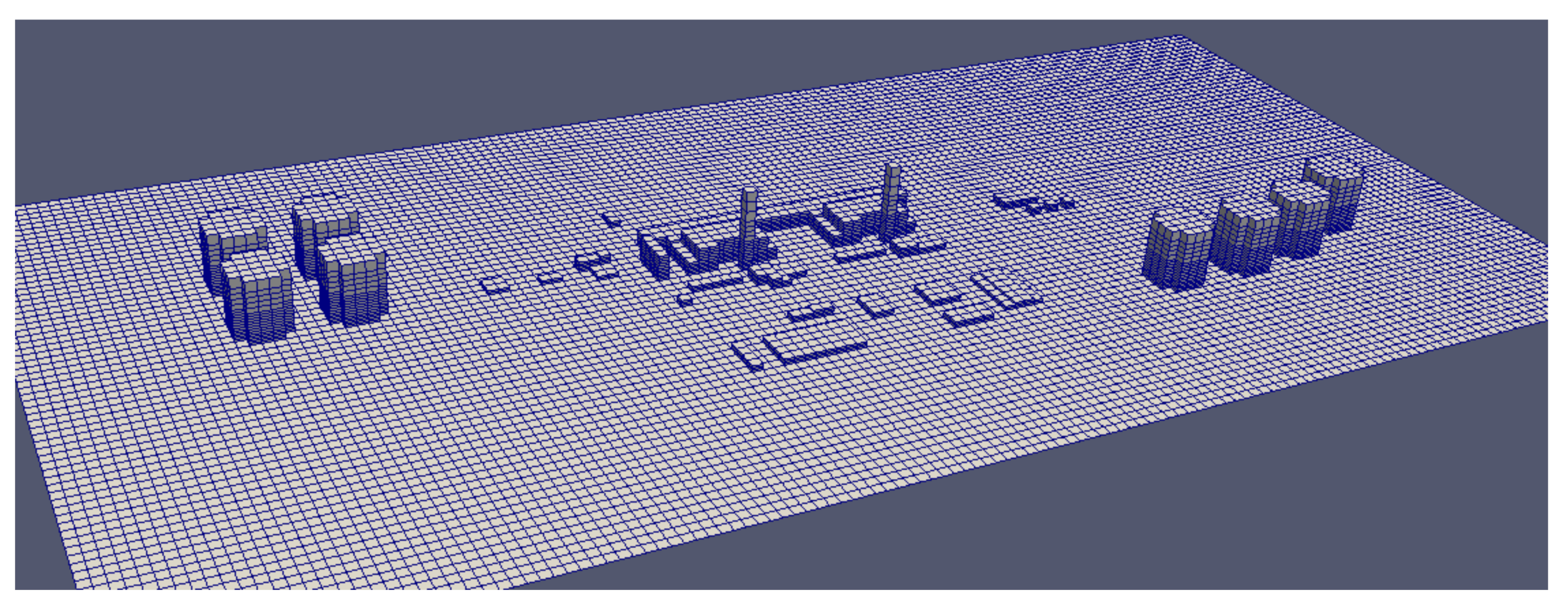
The described 3D urban approach in the area of a nuclear power plant was applied in the ESTE system implementation at the Mochovce NPP in Slovakia. The area is non-trivial from the point of view of the present build-up area: there are buildings for the four units (two in operation and two in the final phases of construction), eight cooling towers, and many auxiliary buildings.
In real application, the computational meteorological fields are precalculated in the form of a large ensemble, instead of involving the calculation of the wind field during an emergency response (or during crisis center training). Each element of the ensemble is characterized by three parameters (directly observable or derivable from observation):
  • Category stability, for which three cases are taken into account: unstable weather conditions (in that case, the vertical profiles on the boundaries for the calculated fields were specified by Monin–Obukhov length, L = 100 m), neutral weather conditions (L = infinity) and stable weather conditions (L = −100 m).
  • Wind direction: taking into account 36 different wind directions (with a uniform step of 10°). The wind direction specifies direction of the wind entered into the meteorological field calculation as a boundary condition.
  • Wind speed: taking into account 40–50 values of wind speed (depending on the stability category), ranging from low wind speed of about 0.2 m/s to 9 m/s (stable weather), to 25 m/s (neutral and unstable weather). The wind speed means the wind rate at the height of 10 m in the specification of the boundary condition for calculation of the meteorological fields.
In the 3D model of Mochovce NPP, the computational area is discretized on cells with a size of 20 m × 20 m. The whole domain has a size of 2800 m × 1400 m. A visualization of the 3D model is shown in Figure 1.
The Lagrangian dispersion model for urban environment is based on theoretical description of [9,20]. The basic transport equations of the urban LPM are again Equation (1). Here, the mean wind of Equation (1) represents the averaged wind over a specific time interval (10 min) in the computational domain, and the mean wind is calculated as a solution of the Navier–Stokes equations.
The vector ui in (1) represents the random walk term of the wind. The diffusion term in Equation (2) obtains a simple form:
bij = (C ε dt)1/2 δij
where C is a universal constant, ε is the mean turbulent kinetic energy dissipation rate and is one outcome of Equation (11), dt is the time step, and δij is Kroneker delta. The drift term from Equation (2) is calculated as the Thompson’s simplest solution for diffusion in three dimensions. It is a function of the Reynolds stress tensor τ, another outcome of Equation (11), but it is more technical, therefore for more details we refer to [9,20]. This approach is implemented in several other urban dispersion models as well, e.g., the QUICPLUME model [21].
The outcome of the dispersion simulation was a concentration of airborne radionuclides and deposited material. Dry deposition Add on a surface is calculated using a similar approach as described above in (2), except for the inclusion of the surface orientation parameter cso:
Add = C0 νd cso.
For example, cso for aerosols is equal to 1 if the surface normal is vertical, and it is equal to 0.1 if the surface normal is oriented horizontally [22,23]. C0 is the air concentration in the particular cell whose surfaces are considered as they undergo contamination by deposition. The evaluation of wet deposition takes into account all cells above the particular horizontal surface, but the vertical surfaces are assigned as zero wet deposition.
The radiological parameters are calculated for ground cells, i.e., cells having at least one ground or building surface. Such cells are potential locations for being occupied by persons. In the case of committed effective dose by inhalation, the instant dose rate DRinhal and the integral dose Dinhal for a particular cell are calculated using Equations (5) and (6), but with C0 as the actual air concentration in the given cell and Cint as the time-integrated concentration in that cell.
The dose rate in the case of an external dose by cloudshine is calculated as a sum of the contribution of all cells j to the dose for the particular cell i as follows:
DRcloud (i) = ∑_j C0 (j) CFcloud (i,j) SF(i,j)
where C0(j) is the air concentration in the contributing cell, SF is shielding factor (equal to 1 if there is no building along a straight line between the cell centers of i and j, and equal to 0 if there is a building), CFcloud is the conversion factor for cloudshine, as a function of the nuclide and of the distance between cell centers i and j.
Similarly, the dose rate of the external dose by deposition is calculated as a sum of contribution of all ground and building surfaces j to the dose for the particular cell as follows:
DRdepo (i) = ∑_j D0 (j) CFdepo (i,j) SF(i,j)
where D0(j) is the deposit on the contributing cell. SF is shielding factor (equal to 1 if there is no building along a straight line between the cell centers of i and j, and equal to 0 if there is a building), CFdepo is the conversion factor for the external dose via deposition, as a function of the nuclide and of the distance between cell centers i and j. The factors CFcloud and CFdepo are prepared as a precalculated library (prepared by calculation using MCNP code version 5 [24]), for various distances between the cells and various cell sizes.
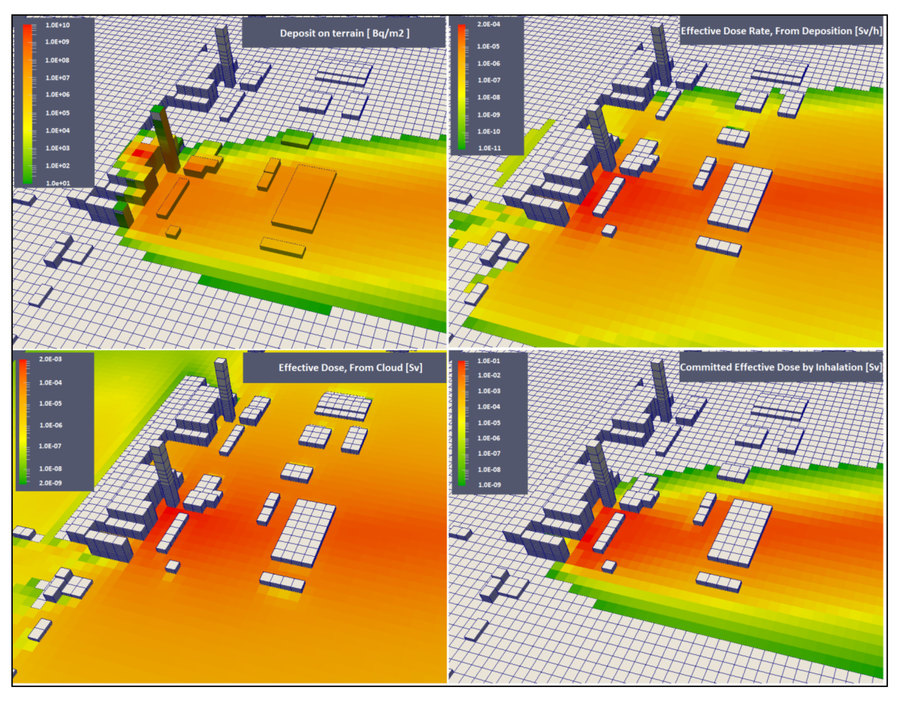
An example of results for a release in an urban environment is shown in Figure 2. The simulation was done for a release of 1.0 × 10¹⁵ Bq of Cs-137 from the roof of the reactor building. Shown is the deposit on all surfaces (buildings and ground), the effective dose rate corresponding to this deposit, the effective dose rate from the cloud during the duration of the release, and the committed effective dose by inhalation. Doses and dose rate were calculated for ground cells.

3. Analysis and Discussion of Calculation Settings for LPM in Mesoscale Impacts

A description of specific assumptions of the LPM set up in ESTE is in Section 2.1, namely: (i) the influence of the total number of modeled particles, (ii) the influence of the initial spatial distribution of the released particles, and (iii) the influence of the height of the bottom reference layer of air. These aspects could influence the results of the modeled dispersion, and especially the calculated radiological impacts. All three aspects were analyzed, and are presented consecutively in Section 3.1, Section 3.2 and Section 3.3.
All the analyses performed in this section shared the same basic inputs. The release event was situated at the Bohunice NPP in Slovakia. The site represents a general European inland nuclear site from the point of view of the analyzed aspects. Another location would be equally applicable for the analyses.
We assumed a release of 1.0 × 10¹⁵ Bq of Cs-137, beginning at 10:00 (UTC) on November 9 and lasting 1 h. The size of the release was chosen to obtain non-negligible radiological impacts, but the choice of the size itself had no qualitative impact on the studied aspects. The southern wind was predominant during the hypothetical release, and there were slightly rainy conditions during the atmospheric transport phase, so dry and wet deposits were present in the modeled calculations. The height of the release point was set to 80 m above ground. The applied meteorological data were the numerical weather-prediction data as predicted by ECMWF for 9–16 November 2020. The dispersion in the atmosphere and the radiological impacts up to seven days from the release time were modeled.
The analyzed properties were studied in a set of locations, which were chosen to lie approximately along the transport of the main activity. The analyses were performed for these six locations:
  • Point1—the village of Nižná, Slovakia, located about 4 km from the release location.
  • Point2—the village of Prašník, Slovakia, located about 17 km from the release location.
  • Point3—the village of Strání, Czech Republic, located about 45 km from the release location.
  • Point4—the town of Valašské Meziříčí, Czech Republic, located about 110 km from the release location.
  • Point5—Warsaw, Poland, located about 480 km from the release location.
  • Point6—Rovno, Ukraine, located about 665 km from the release location.
In the case of analyzing integrated paths, or trajectories, starting from the defined release point and time in the given field of NWP data and leading in specific heights, the first five points were chosen to lie near the trajectory related to the assumed release height (Figure 3). The appropriateness of the choice of these five points was also approved by studying the impacts of dispersion calculation. The choice of Point6 was justified according to the impact calculation—one of the most impacted regions at larger distances (see map of impacts in the following section). Point5 and Point6 are at a similar direct distance from the release point (about 500–600 km), but the trajectories of radionuclides dispersed to Point6 were longer than 1000 km.

3.1. Total Number of Modeled Particles

In the case of ESTE designed for nuclear crisis centers, the time limit for availability of calculated radiological impacts of a predicted release was 15 min. The number of particles was set to 250,000 in the ESTE system to meet the time limit. The results of the analysis of the influence of particle number on the ground deposit for Cs-137 are presented in Table 3. The map of the resulting total ground deposit of Cs-137 is displayed in Figure 4, and the map of the resulting wet deposit of Cs-137 in Figure 5. Supplementary to Figure 4 and Figure 5, an evolution of total and wet deposit of Cs-137 over time on the map of Europe is presented in video S1 and video S2.
The number of particles applied in the study was set to 25,000, 100,000, 250,000, and 1,000,000. All calculations were performed using the parallel computing platform CUDA, exploiting a graphics purpose unit (GPGPU). The respective times of calculations were 8 min, 9 min, 11 min, and 22 min. The LPM dispersion mesh had the resolution of 0.025° × 0.025°, i.e., a resolution with a size of about 2–3 km. The presented results are at points 2, 3, 4, 5, and 6. From the results in Table 3a,b, it is evident that when distances up to hundreds of km are taken into account, the results of a release simulated by 100,000 particles or higher are well converged and lead to little fluctuating results of ground deposit in the test. Large and random fluctuations of ground deposit, and, implicitly, of any other radiological parameter, are evident in case of larger distances.
The conclusion for the number of particles applied in the LPM of the ESTE system is that 250,000 particles for distances at the level of hundreds of kilometers is an appropriate and adequate number. At the same time, if dispersion along trajectories at the level of 1000 kilometers or more is modeled, then a much higher number of particles than 250,000 should be applied.

3.2. LPM: Initial Spatial Distribution of Released Particles

The decision-support systems running in nuclear crisis centers, like the ESTE system, are tasked with predicting and assessing the radiation situation in close vicinity to the release. It is a task of higher importance than the mesoscale dispersion, since the population in close vicinity is the most exposed to the release. Close vicinity means the area of the nuclear facility and the emergency planning zone, which usually has a radius of about 15 to 30 km. For calculation of impacts at distances at the level of the emergency planning zone, an assumption about the initial spatial distribution of the source plays a non-negligible role. The influence of the initial spatial distribution of the source was analyzed, and the results are reported in Table 4.
In the analysis, we assumed the following types of source: (a) a point source at 80 m, meaning that the starting height of all particles was set to the height of 80 m above ground; (b) a line source at 80 ± 20 m, meaning that the starting height of particles was uniformly generated between 60 m and 100 m; (c) a line source with 125 ± 20 m means a uniform generation of particles between the heights 105 m and 145 m; and (d) a line source with 35 ± 10 m means a uniform generation of particles between the heights 25 m and 45 m above the ground. All defined sources reflected specific uncertainties in the release height occurring in the dispersion simulations: (a) limited knowledge about the right release point—the release could happen through various building structures, walls or roofs; and (b) limited knowledge about the release conditions—the volume of air from containment undergoes thermal and pressure changes when released to the atmosphere and leading, e.g., plume rising.
Since we focused on the closest points in this analysis, the presented results are at the points 1, 2, 3, 4, and 5. The conclusion from the results (Table 4) was that the influence of the initial spatial distribution of the source of particles on the impacts calculated is significant at distances close to the source of release (e.g., for point 1, lying 4 km from the release point). At distances above 20 km from the source, the initial spatial distribution and height of the source above the ground had a small or negligible influence on the results.
Naturally, we are dealing with a different situation when the released radionuclides are lifted to a great height; for example, due to an explosion. In such a case, due to the potentially different wind directions at higher heights of the atmosphere, the trajectories of particles lifted to higher heights from the terrain can be completely different from a leak at ground level. A demonstration of this phenomenon is shown in Figure 3. In the ESTE decision-support system, the initial spatial distribution of particles is one attribute of the source term. The source term is assessed either by the ESTE system itself, or is a part of the information from the damaged nuclear facility.

3.3. LPM: Height of the Bottom Reference Layer of Air

The height of the bottom reference layer of air above ground could affect calculated impacts near a nuclear facility in which a release took place. In the LPM of the ESTE system, the height of the bottom layer of air was set to 100 m. The influence of the assumed height of the bottom layer of air was studied, and the results are reported in Table 5.
The presented results are at points 1, 2, 3, 4, and 5. The conclusion from the results in Table 5 is that the influence of the model-applied height of the bottom layer of air above the ground was not significant. The effect of the modeled bottom-layer height could be significant if the number of particles is low. Such a situation could occur if the total number of applied particles in the calculation is low. In our analysis, we applied 250,000 particles, so we did not expect to see an influence on the results, at least in the vicinity of about 100 km from the source. But if we analyze points or regions further from the source where the concentration of particles is low, a non-negligible influence could be observed on the calculated parameters, e.g., Point5.

4. Conclusions

The ESTE system is a decision-support system for nuclear crisis centers that estimates the source term based on the known or evaluated state of the facility’s systems, and models atmospheric transport of radioactive material leaked to the atmosphere as a result of an accident at a nuclear facility. The dispersion models of ESTE, which cover modeling of dispersion in mesoscale up to a global range, as well as dispersion in microscale, meaning transport in urban and industrial environments, have been described. Modeling transport and dispersion on mesoscale were performed by implementing the Lagrangian particle model and the Puff trajectory model. Both models were adequate for radiological-impact assessment in the vicinity of a nuclear facility and for recommending measures for protecting the population. The Lagrangian particle model, being more detailed in modeling the dispersion phenomena, allowed a more reliable simulation, even on a global scale, as it was shown on the basic estimation of transport time for central Europe sourced from the Fukushima disaster. The impact calculation must be based on numerical weather-prediction data.
In the case of dispersion and radiological impact-modeling in an urban environment, the calculation was based on the Lagrangian particle model analogously. Additionally, the calculation required the capability to compute the urban wind fields in that case, due to very specific meteorological conditions in each urban area. In both the urban environment and at the atmospheric mesoscale scale, the ESTE system performed assessments of the impacts on the population and suggested countermeasures.
The parameters of the models were set so that the calculations for emergency situations could be performed with high accuracy in a relatively short time, within about 15 min. Several parameters were presented and discussed to be set in the ESTE system acceptably and adequately in the mesoscale case: (i) the number of applied particles in the calculation allowed for accurate results in some minutes for distances up to about 1000 km, (ii) detailed knowledge of the initial spatial distribution of the source played a more important role in close vicinity of the release, and was less influential at larger distances, and (iii) the height of the bottom reference layer showed a small influence on accuracy in the case of applying a sufficiently large number of particles.

Supplementary Materials

The following are available online at https://0-www-mdpi-com.brum.beds.ac.uk/2073-4433/12/2/204/s1. Video S1: Ground deposits of Cs-137 as a result of the release of 1 × 10¹⁵ Bq of Cs-137 from Bohunice NPP at 10:00 UTC on 9 November 2020. Evolution of total deposits over time on the map of Europe in time steps: 8 h, 16 h, 24 h, 2 days, 3 days, 4 days, 5 days, 6 days, and 7 days from the time of release; Video S2: Ground deposits of Cs-137 as a result of the release of 1 × 10¹⁵ Bq of Cs-137 from Bohunice NPP at 10:00 UTC on 9 November 2020. Evolution of wet deposits over time on the map of Europe in time steps: 8 h, 16 h, 24 h, 2 days, 3 days, 4 days, 5 days, 6 days, and 7 days from the time of release; Video S3: The Fukushima Dai-ichi catastrophe, radiological impacts to Central Europe modeled by the LPM of ESTE. Time integral of air concentration (TIC) of I-131 in the bottom layer of the atmosphere up to the 16 days from the beginning of release. The blue color represents particles dispersed from Fukushima in all levels of the atmosphere—from the terrain up to >5 km above the terrain.

Author Contributions

Conceptualization, Ľ.L., P.Č., E.F. and M.K.; methodology, Ľ.L. and P.Č.; software, Ľ.L., P.Č. and E.F.; validation, P.Č. and Ľ.L.; investigation, Ľ.L., P.Č., E.F. and M.K.; data curation, V.F. and Ľ.L.; writing—original draft preparation, M.K., Ľ.L. and P.Č.; visualization, V.F. and Ľ.L.; supervision, P.Č., Ľ.L. and M.K. All authors have read and agreed to the published version of the manuscript.

Funding

This research received no external funding and was fully funded from internal resources of the company ABmerit, Ltd., where the authors are employed.

Acknowledgments

The authors would like to thank the Austrian Crisis Center at the Division 8—Radiation Protection of the Austrian Federal Ministry for Climate Action, Environment, Energy, Mobility, Innovation and Technology (BMK) for kindly allowing the partial calculations and analyses presented in this article to be performed on ESTE computers at the Center and with data available from the ESTE system of the Center.

Conflicts of Interest

The authors declare no conflict of interest.

References

  1. Fojcíková, E.; Lipták, Ľ.; Krpelanová, M.; Chylý, M.; Čarný, P. ESTE—Decision Support System for Nuclear and Radiological Accidents. Radiat. Prot. Dosim. 2019, 186, 321–325. [Google Scholar] [CrossRef] [PubMed]
  2. McKenna, T.J.; Glitter, J.G. Source Term Estimation During Incident Response to Severe Nuclear Accidents; NUREG-1228; Nuclear Regulatory Commission: Washington, DC, USA, 1988.
  3. Generic Assessment Procedures for Determining Protective Actions during a Reactor Accident; IAEA-TECDOC-955; IAEA: Vienna, Austria, 1997.
  4. Response Technical Manual; NUREG/BR-0150; U.S. Nuclear Regulatory Commission: Rockville, MD, USA, 1995.
  5. RASCAL 4.0: Description of Models and Methods; NUREG-1940; U.S. Nuclear Regulatory Commission: Washington, DC, USA, 2012.
  6. OECD/NEA; Committee on the Safety of Nuclear Installations. Benchmarking of Fast-Running Software Tools Used to Model Releases During Nuclear Accidents; NEA/CSNI/R(2015)19; OECD/NEA: Paris, France, 2016. [Google Scholar]
  7. Oak Ridge National Laboratory. SCALE—Comprehensive Modeling and Simulation Suite for Nuclear Safety Analysis and Design. Available online: www.ornl.gov/scale (accessed on 2 February 2021).
  8. IAEA. PRIS: Power Reactor Information System (Database of the IAEA). Available online: http://prisweb.iaea.org (accessed on 2 February 2021, for registered user).
  9. Thomson, D.J. Criteria for the Selection of Stochastic Models of Particle Trajectories in Turbulent Flows. J. Fluid Mech. 1987, 180, 529–556. [Google Scholar] [CrossRef]
  10. Stohl, A.; Forster, C.; Frank, A.; Seibert, P.; Wotawa, G. Technical Note: The Lagrangian Particle Dispersion Model FLEXPART Version 6.2. Atmos. Chem. Phys. 2005, 5, 2461–2474. [Google Scholar] [CrossRef] [Green Version]
  11. Baumann Stanzer, K.; Skomorowski, P.; Polreich, E. Comparison of TAMOS/ESTE/RODOS Results; Technical Report; ZAMG, Zentralanstalt für Meteorologie und Geodynamik: Vienna, Austria, 2014. [Google Scholar]
  12. IAEA-Document: The Fukushima Daiichi Accident; Volume 4/5: Radiological Consequences; International Atomic Energy Agency: Vienna, Austria, 2015.
  13. Rulík, P.; Hýža, M.; Bečková, V.; Borecký, Z.; Havránek, J.; Hölgye, Z.; Lušňák, J.; Malá, H.; Matzner, J.; Pilátová, H.; et al. Monitoring Radionuclides in the Atmosphere over the Czech Republic after the Fukushima Nuclear Power Plant Accident. Radiat. Prot. Dosim. 2015, 163, 226–232. [Google Scholar] [CrossRef] [PubMed]
  14. Skulec, Š.; Ďúran, J.; Slaby, J.; Janiskova, M. Influence of Complex Terrain on Mathematical Modeling of Emissions Dispersion from Industrial Plants in Slovakia and Czechoslovakia; Slovak Hydrometeorological Institute and Slovak Academy of Sciences: Bratislava, Slovakia, 1988; (In Slovak Language). [Google Scholar]
  15. Zannetti, P. Air Pollution Modeling: Theories, Computational Methods, and Available Software; Van Nostrand: New York, NY, USA, 1990. [Google Scholar]
  16. Lipták, Ľ.; Fojcíková, E.; Čarný, P. Comparison of the ESTE CBRN Model with the Joint Urban 2003 Experiment. Bound. Layer Meteorol. 2019, 171, 439–464. [Google Scholar] [CrossRef]
  17. Patankar, S.V.; Spalding, D.B. A Calculation Procedure for Heat, Mass and Momentum Transfer in Three-Dimensional Parabolic Flows. Int. J. Heat Mass Transf. 1972, 15, 1787–1806. [Google Scholar] [CrossRef]
  18. Launder, B.E.; Spalding, D.B. The Numerical Computation of Turbulent Flows. Comput. Methods Appl. Mech. Eng. 1974, 3, 269–275. [Google Scholar] [CrossRef]
  19. Hanna, S.R.; Briggs, G.A.; Hosker, R.P. Handbook on Atmospheric Diffusion; Technical Report DOE-TIC-11223; Office of Energy Research, U.S. Department of Energy: Washington, DC, USA, 1982.
  20. Rodean, H.C. Stochastic Lagrangian Models of Turbulent Diffusion; The American Meteorological Society: Boston, MA, USA, 1996; 82p. [Google Scholar]
  21. Pardyjak, E.R.; Brown, M. QUIC-URB v. 1.1: Theory and User’s Guide; Los Alamos National Laboratory: Los Alamos, NM, USA, 2003.
  22. Byrne, M.A.; Goddard, A.J.H.; Lange, C.; Roed, J. Stable Tracer Aerosol Deposition Measurements in a Test Chamber. J. Aerosol Sci. 1995, 26, 645–653. [Google Scholar] [CrossRef]
  23. Roed, J. Deposition and Removal of Radioactive Substances in an Urban Area; Final Report of the NKA Project AKTU-245; Risoe National Laboratory: Roskilde, Denmark, 1990; p. 91. [Google Scholar]
  24. Los Alamos National Laboratory. MCNP—A General Monte Carlo N-Particle Transport Code, Version 5, Software Product Produced by Los Alamos National Laboratory. Available online: https://mcnp.lanl.gov/ (accessed on 2 February 2021).
Figure 1. 3D model of the area of the Mochovce nuclear power plant, Slovakia.
Atmosphere 12 00204 g001
Figure 2. Example of an impact calculation for an urban environment—a release from the reactor building of the Mochovce NPP is simulated). Deposit on surfaces (top left), and effective dose rate from deposition (top right), from cloud (bottom left), and by inhalation (bottom right) are shown.
Atmosphere 12 00204 g002
Figure 3. Trajectories, i.e., integrated paths, of the wind field for the initial point of the Bohunice NPP, at 10:00 UTC, 9 November 2020, for three various heights—100 m (blue line), 500 m (green line), and 1500 m (red line) above terrain. The locations of the six studied points are also shown.
Atmosphere 12 00204 g003
Figure 4. Total ground deposit of Cs-137 in +7 days from the time of release. The deposit is a result of the release of 1 × 10¹⁵ Bq of Cs-137 from Bohunice NPP, at 10:00 UTC on 9 November 2020.
Atmosphere 12 00204 g004
Figure 5. Wet deposit of Cs-137 in +7 days from the time of release. The deposit is a result of the release of 1 × 10¹⁵ Bq of Cs-137 from Bohunice NPP, at 10:00 UTC on 9 November 2020.
Atmosphere 12 00204 g005
Table 1. List of isotopes significant in radiological-impact calculations in case of events in a nuclear facility and applied in ESTE models.
Kr85mSr89Zr95Ru105Te127I132Xe133Cs137Ce143Pu241
Kr85Sr90Zr97Ru106Te129mI133Xe135Cs138Ce144
Kr87Sr91Nb95Rh103mTe129I134Xe135mBa140Np239
Kr88Y90Mo99Rh105Te131mI135Xe138La140Pu238
Rb86Y91mTc99mSb127Te132Xe131mCs134Pr143Pu239
Rb88Y91Ru103Sb129I131Xe133mCs136Ce141Pu240
Table 2. The applied Briggs sigma function σ (L) for the horizontal Gaussian model, where L is the travel length.
Stability CategorySigma Function for Urban ConditionSigma Function for Rural Condition
Aσ (L) = 0.32 × L × (1 + 0.0004 × L)−1/2σ (L) = 0.22 × L × (1 + 0.0001 × L)−1/2
Bσ (L) = 0.22 × L × (1 + 0.0004 × L)−1/2σ (L) = 0.16 × L × (1 + 0.0001 × L)−1/2
Cσ (L) = 0.22 × L × (1 + 0.0004 × L)−1/2σ (L) = 0.11 × L × (1 + 0.0001 × L)−1/2
Dσ (L) = 0.16 × L × (1 + 0.0004 × L)−1/2σ (L) = 0.08 × L × (1 + 0.0001 × L)−1/2
Eσ (L) = 0.11 × L × (1 + 0.0004 × L)−1/2σ (L) = 0.06 × L × (1 + 0.0001 × L)−1/2
Fσ (L) = 0.11 × L × (1 + 0.0004 × L)−1/2σ (L) = 0.04 × L × (1 + 0.0001 × L)−1/2
Table 3. Deposit of Cs-137, seven days from the beginning of the release of 1 × 10¹⁵ Bq, in various points as a function of the number of particles modeled. (a) Dry deposit, [Bq/m2], and ratio to dry deposit in the case of 1,000,000 particles; (b) Wet deposit, [Bq/m2], and ratio to wet deposit in the case of 1,000,000 particles.
Number of ParticlesPoint2Point3Point4Point5Point6
(a)
25,0004.3 × 104/0.935.7 × 104/0.987.8 × 103/0.951.2 × 103/1.231.6 × 100/0.23
100,0004.8 × 104/1.035.8 × 104/1.008.1 × 103/0.991.0 × 103/1.067.8 × 100/1.15
250,0004.7 × 104/1.015.9 × 104/1.028.1 × 103/0.999.7 × 102/1.023.5 × 100/0.51
1,000,0004.6 × 104/1.005.8 × 104/1.008.2 × 103/1.009.5 × 102/1.006.8 × 100/1.00
(b)
25,0008.8 × 103/1.031.6 × 105/1.003.2 × 104/0.966.8 × 101/1.081.3 × 100/0.08
100,0008.5 × 103/0.991.5 × 105/0.993.3 × 104/0.996.8 × 101/1.077.7 × 100/0.49
250,0008.6 × 103/1.001.6 × 105/1.003.3 × 104/0.996.4 × 101/1.011.5 × 101/0.94
1,000,0008.6 × 103/1.001.6 × 105/1.003.4 × 104/1.006.3 × 101/1.001.6 × 101/1.00
Table 4. Deposit of Cs-137, seven days from the beginning of the release of 1 × 10¹⁵ Bq, in various points, as a function of initial spatial distribution of the source. Dry deposit, [Bq/m2], and ratio to dry deposit in case of point source at 80 m.
Spatial Distribution of the SourcePoint1Point2Point3Point4Point5
point at 80 m4.4 × 105/1.001.0 × 105/1.005.9 × 104/1.008.1 × 103/1.009.7 × 102/1.00
line with 80 ± 20 m3.9 × 105/0.881.0 × 105/1.015.8 × 104/0.988.1 × 103/1.009.6 × 102/0.99
line with 125 ± 20 m3.2 × 105/0.731.0 × 105/1.046.1 × 104/1.038.5 × 103/1.051.0 × 103/1.08
line with 35 ± 10 m4.3 × 105/0.971.0 × 105/1.005.7 × 104/0.978.1 × 103/1.009.4 × 102/0.97
Table 5. Deposit of Cs-137, seven days from the beginning of the release of 1 × 10¹⁵ Bq, in various points, as a function of the height of the bottom layer of air. Dry deposit, [Bq/m2], and ratio to dry deposit in the case of a 100 m layer.
Bottom Layer of AirPoint1Point2Point3Point4Point5
100 m layer4.4 × 105/1.004.7 × 104/1.005.9 × 104/1.008.1 × 103/1.009.7 × 102/1.00
50 m layer4.1 × 105/0.944.5 × 104/0.975.7 × 104/0.978.1 × 103/1.008.8 × 102/0.91
25 m layer4.2 × 105/0.954.6 × 104/0.985.6 × 104/0.958.2 × 103/1.018.5 × 102/0.88
Publisher’s Note: MDPI stays neutral with regard to jurisdictional claims in published maps and institutional affiliations.

