
Model Uncertainty in the Projected Indian Summer Monsoon Precipitation Change under Low-Emission Scenarios


1
Key Laboratory of Marine Hazards Forecasting, Ministry of Natural Resources/Key Laboratory of Ministry of Education for Coastal Disaster and Protection, College of Oceanography, Hohai University, Nanjing 210098, China
2
Southern Marine Science and Engineering Laboratory (Zhuhai), Zhuhai 519082, China
*
Author to whom correspondence should be addressed.
Atmosphere 2021, 12(2), 248; https://0-doi-org.brum.beds.ac.uk/10.3390/atmos12020248
Submission received: 30 December 2020
/
Revised: 4 February 2021
/
Accepted: 6 February 2021
/
Published: 12 February 2021
(This article belongs to the Special Issue Asian Summer Monsoon Variability, Teleconnections and Projections)
Abstract
:The projected ISM precipitation changes under low-emission scenarios, Representative Concentration Pathway 2.6 (RCP2.6) and Shared Socioeconomic Pathway 1-2.6 (SSP1-2.6), are investigated by outputs from models participating in phases 5 and 6 of the Coupled Model Intercomparison Project (CMIP5 and CMIP6). Based on the high-emission scenarios like RCP8.5, the Intergovernmental Panel on Climate Change Fifth Assessment Report suggests a wetter Indian summer monsoon (ISM) by the end of 21st century. Although the multi-model ensemble mean (MME) ISM precipitation under RCP2.6 and SSP1-2.6 is still projected to increase over 2050–2099 referenced to 1900–1949, the intermodel spread of the ISM precipitation change is tremendous in both CMIPs. Indeed, the signal-to-noise ratio (SNR) of ISM precipitation change, defined as the MME divided by its intermodel standard deviation, is even below 1 under the low-emission scenarios. This casts doubts on a future wetter ISM in a warmer climate. Moisture budget analyses further show that most of the model uncertainty in ISM precipitation change is caused by its dynamical component from the atmospheric circulation change. As expected, the interhemispheric surface warming contrast is essential in causing the intermodel differences in ISM circulation and precipitation changes under low-emission scenarios. In addition, the projected wetter ISM is prominently enhanced from CMIP5 to CMIP6, along with reduced model uncertainty. However, the resultant increased SNR in CMIP6 is still low in most ISM regions. The results imply that ISM precipitation change is highly uncertain under low-emission scenarios, which greatly challenges the decisions-making in adaptation policies for the densely populated South Asian countries.
1. Introduction
The Indian summer monsoon (ISM), or south Asian summer monsoon, is one of the most striking monsoon systems on earth, which typically lasts from June to September and brings a large amount of moisture to the Indian subcontinent and its surrounding regions. Therefore, its variability or change can substantially affect the wet and drought events, food security and human health over densely populated South Asian countries. Future changes of ISM precipitation under global warming can exert pronounced impacts for regions being vulnerable for water supplies. However, large uncertainty lies in the projected precipitation change [1,2,3,4,5,6,7,8], lowering the reliability of models’ future projections [9] and causing a great challenge for adaptation planning.
Model uncertainty, measured by the spread of multiple models’ projections, is deemed the major source of uncertainty in long-term precipitation response to global warming at both global mean and regional spatial scales [10,11,12,13]. This is because climate models display striking differences in projecting both the sign and magnitude of precipitation change [5,6,14]. These differences originating from the reality that models differ in, for example, physical and numerical formulations, parameterization schemes, horizontal and vertical resolutions and tunning method [15,16,17]. Model uncertainty in the projected ISM precipitation change may arise from model biases in simulating the Indian Ocean (IO) climatology [9,16,18,19,20,21,22,23], climate variability [1,24,25], sea surface temperature warming pattern [4,6,7] and associated water vapor and atmospheric circulation changes [7,26].
Under global warming, the increased atmospheric water vapor due to enhanced surface evaporation is supposed to increase precipitation everywhere [27]. However, the advection of moisture by atmospheric circulation complicates the precipitation responses at different regions. The climatological circulation and circulation change both strongly shape the spatial structure of future precipitation change [7,26,28,29]. For example, despite the fact that the increased moisture would promote ISM precipitation [30,31,32], a possibly weakened ISM due to a reduced upper tropospheric temperature gradient can largely suppress the precipitation increase [2,33]. The inconsistency in projected moisture increase and atmospheric circulation changes is termed a paradox of ISM response to global warming [31,33,34], which is an important source of the model-to-model differences in ISM precipitation change.
To understand the underlying mechanisms controlling the precipitation response and its model uncertainty, precipitation change is usually diagnostically decomposed into the sum of evaporation change, a thermodynamical component due to moisture change and a dynamical component due to atmospheric circulation change [7,26,29,32]. Under high-emission scenarios, like Representative Concentration Pathway 8.5 (RCP8.5) where radiative forcing (RF) increases monotonically, the ISM precipitation is projected to increase in nearly all models [3,35]. The thermodynamical component consistently leads to precipitation increase over ISM regions among models, while the dynamical component may dampen or promote the precipitation increase due to monsoon circulation slowdown and displays large intermodel spread and regional variations [4,32]. As a result, intermodel differences in the atmospheric circulation change and thus dynamical component dominates the intermodel spared in precipitation change under high-emission scenarios [6,7,32].
Most previous studies on ISM precipitation projections and model uncertainty are based on middle- and high-emission scenarios, which design no decrease in RF and lead to a high rate of global warming through 2100 in phases 5 and 6 of the Coupled Model Intercomparison Project (CMIP5 and CMIP6). In comparison, RF is designed to decrease in the near future under low-emission scenarios and leads to a weak global warming by 2100. Recently, concerns on the climate responses under the low-emission or low-warming scenarios motivate studies on global and regional climate changes [36,37,38,39,40,41], especially after the 2015 Paris Agreement. These studies imply that the spatial patterns and underlying mechanisms of regional climate responses are substantial different between low- and high-emission scenarios [3,36,41,42,43,44]. However, the ISM precipitation response and associated model uncertainty under low-emission scenarios have not been systematically studied.
Therefore, the present study investigates the model uncertainty in ISM precipitation change by outputs from 25 models under RCP2.6 in CMIP5 and 30 models under Shared Socioeconomic Pathway 1-2.6 (SSP1-2.6) in CMIP6 [45,46]. The ISM precipitation change over 2050–2099 referenced to 1900–1949 is investigated, with a focus on its model uncertainty as the intermodel spread in ISM change is supposed to be significant under weak RF. This may lead to distinct decisions in adaptation policies compared to those under high-emission scenarios for South Asian countries. The comparison between results from CMIP5 and CMIP6 are further explored as the two CMIPs displaying large differences in cloud simulation, parameterization, resolution, etc.
The rest of this paper is organized as follows. Section 2 describes the CMIP model outputs used in the present study. Section 3 compares the MME ISM precipitation response in CMIP5 and CMIP6. Section 4 investigates the origins of the model uncertainty in ISM precipitation change and the underlying mechanisms. Section 5 is a summary with discussions.
2. Datasets and Models
2.1. Model Simulations and Outputs
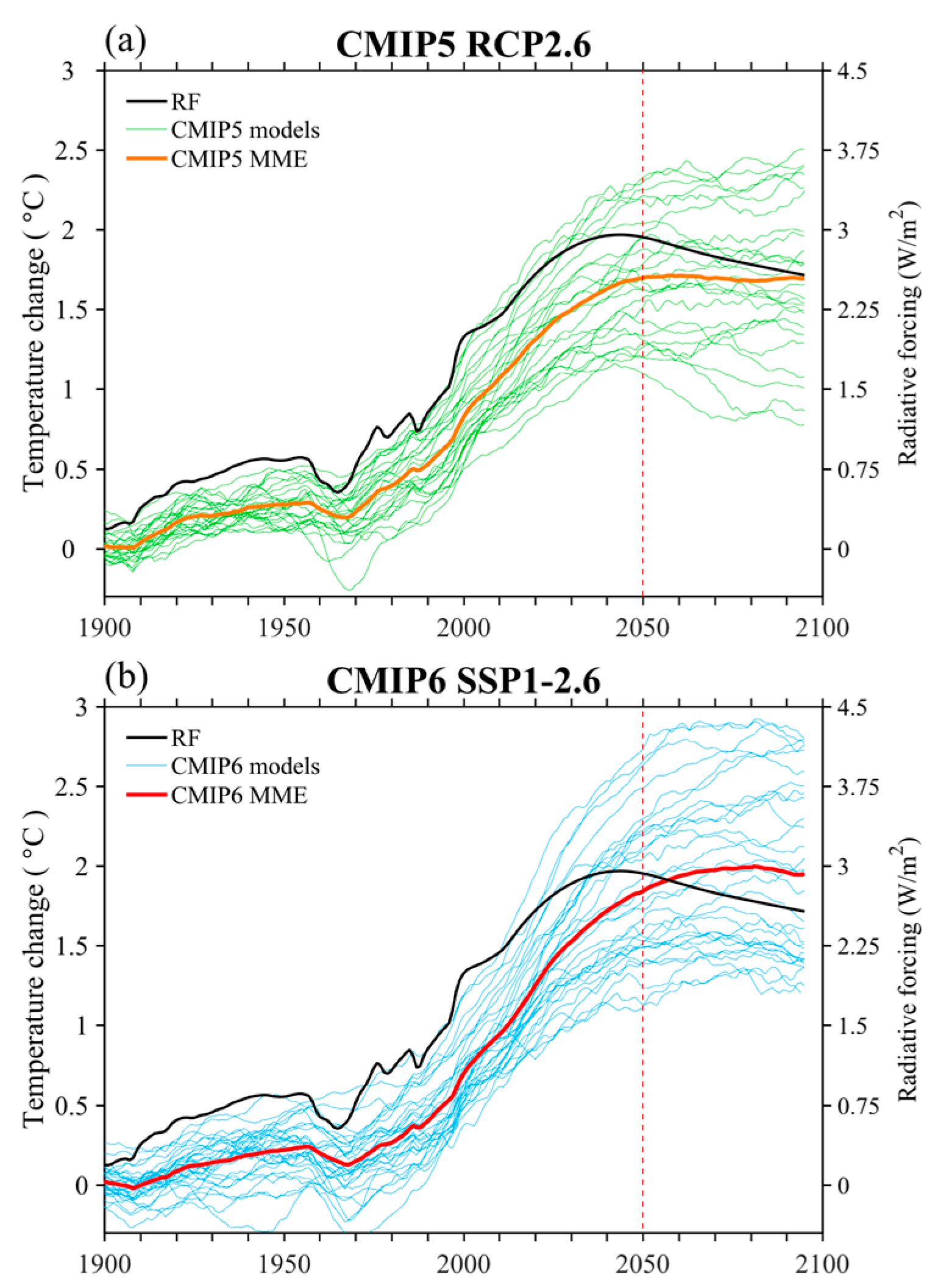
The model outputs from simulations of historical period and future low-emission scenarios, RCP2.6 and SSP1-2.6 [45,46], are analyzed in the present study. The model outputs analyzed in the present study are all based on global earth system models or climate models. In both RCP2.6 and SSP1-2.6, RF is prescribed to first increase to a peak around 2045 and then decrease (Figure 1, black lines). During 2050–2100, the multi-model ensemble mean (MME) global mean surface temperature (GMST) change is weak, the GMST trajectory holds nearly flat in CMIP5 and slightly increases in CMIP6 [41]. Note that there is pronounced differences in the GMST responses between CMIP5 and CMIP6, possibly due to differences in models’ climate sensitivity to external forcing like greenhouse gases and aerosols and cloud simulations [47].
Monthly mean outputs of 25 models from CMIP5 and 30 models from CMIP6 (Table 1), including surface temperature, precipitation, evaporation, vertical velocity and winds are used. Some models conduct several members of the historical and scenario experiments, to ensure equal weight, only one member of each CMIP model is analyzed to ensure equal weight. All model outputs are interpolated onto a common 2° longitude × 2° latitude grid by linear method for easy comparison, the analyses based on the interpolated grids cause only slight differences from those based on model’s original grids over ISM regions (not shown).
2.2. Method
In the present study, the changes in ISM precipitation and associated variables are calculated by subtracting the June–July–August–September (JJAS) mean in 1900–1949 (historical period) from that in 2050–2099 (future period). It is clear that the magnitude of GMST increase after 2050 significantly differs between models and shows larger magnitude in CMIP6 than CMIP5 (colored thin lines in Figure 1a, b). To eliminate the effect of the differences in GMST on the model uncertainty, the GMST increase during 2050–2099 under RCP2.6 or SSP1-2.6 referenced to 1900–1949 is first calculated. For each model, all future changes are then normalized by its GMST increase. Thus, the normalized changes indicate the responses per 1K of global mean surface warming, which mainly focus on the uncertainty in the spatial variation of ISM precipitation change [7,35].
The magnitude of model uncertainty is estimated by the intermodel standard deviation (STD) of MME. To trace the source of the uncertainty in ISM precipitation change, the moisture budget analysis is applied in the present study to diagnostically decompose precipitation change into the sum of different components [7,26]:
The denote the future change, , , , , and are precipitation, evaporation, the thermodynamical component due to moisture change, the dynamical component due to atmospheric circulation change and the residual term, respectively. In the tropics, the thermodynamical and dynamical components can be well approximated as [7,26,29,35]:
where , , and are water density, pressure velocity at 500 hPa and surface specific humidity, respectively. The 500 hPa pressure surface may not be available over part of high mountain regions such as the Tibet plateau, but this issue causes negligible influences on the analyses over the ISM domain analyzed in the present study (65–90° E and 10–30° N, black box in Figure 2).
As surface specific humidity is not available in some models, the vertically integrated water vapor through the atmospheric column () can be used to replace based on the approximation below:
Therefore, Equations (4) and (5) can be estimated by the product of and :
Therefore, uncertainty in the precipitation can be traced into uncertainty from different sources.
3. ISM Precipitation Change
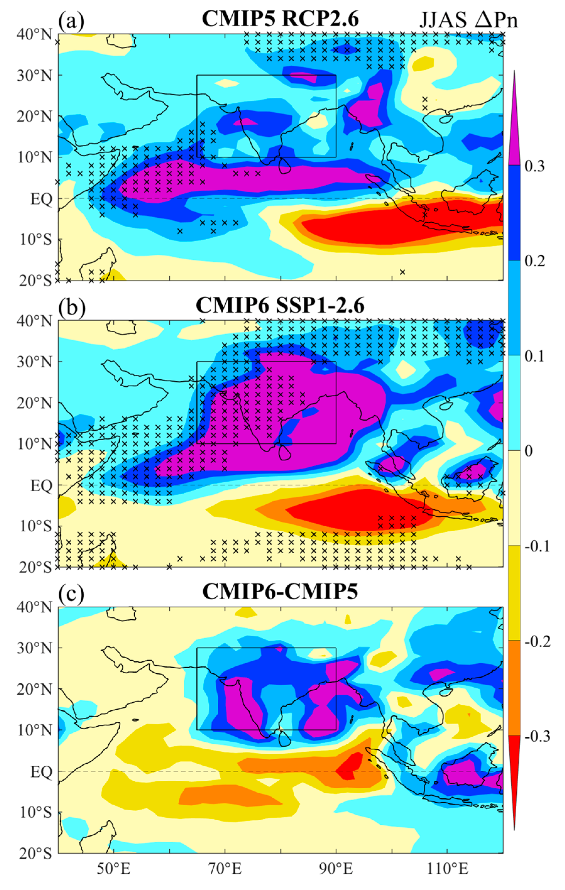
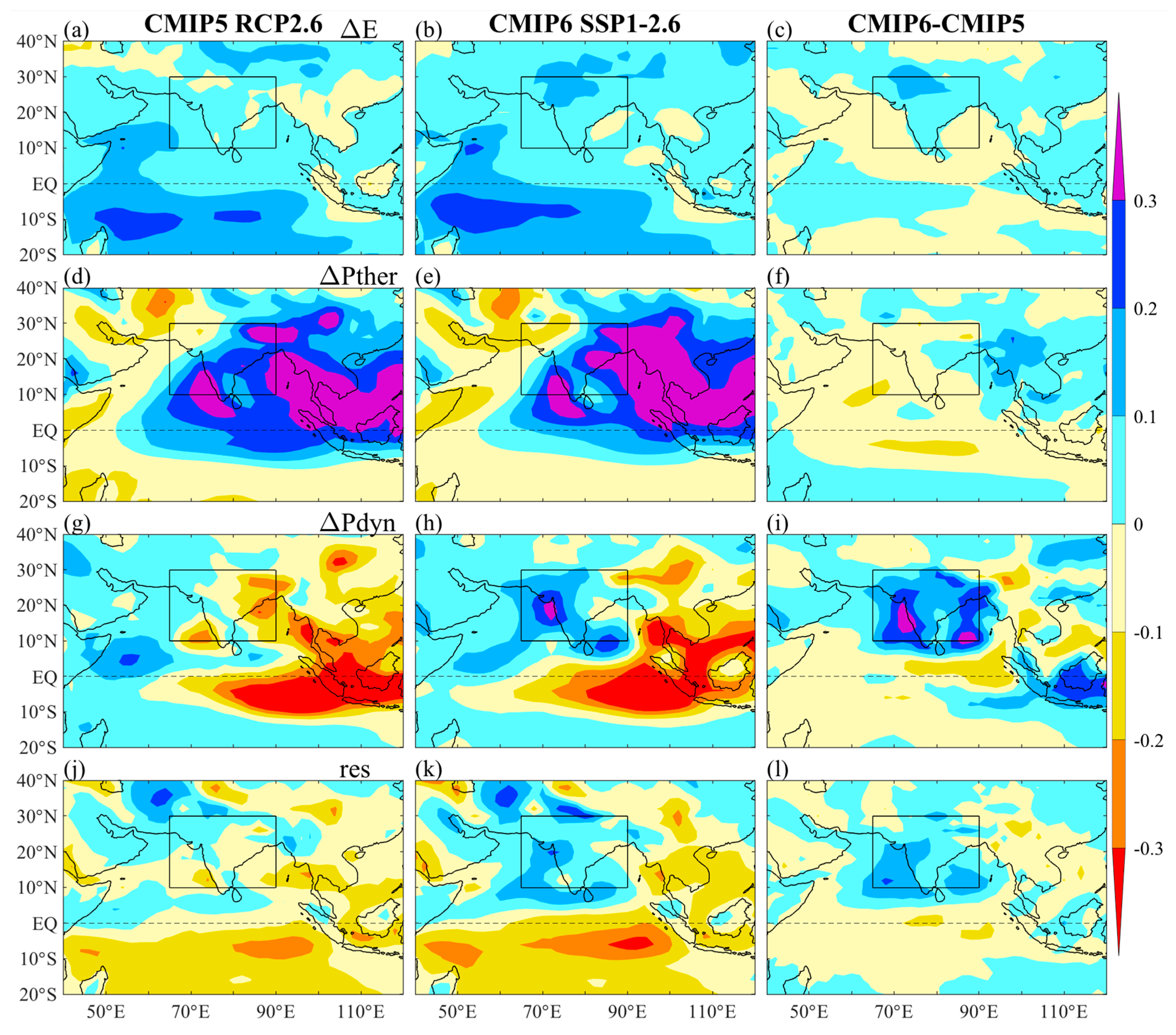
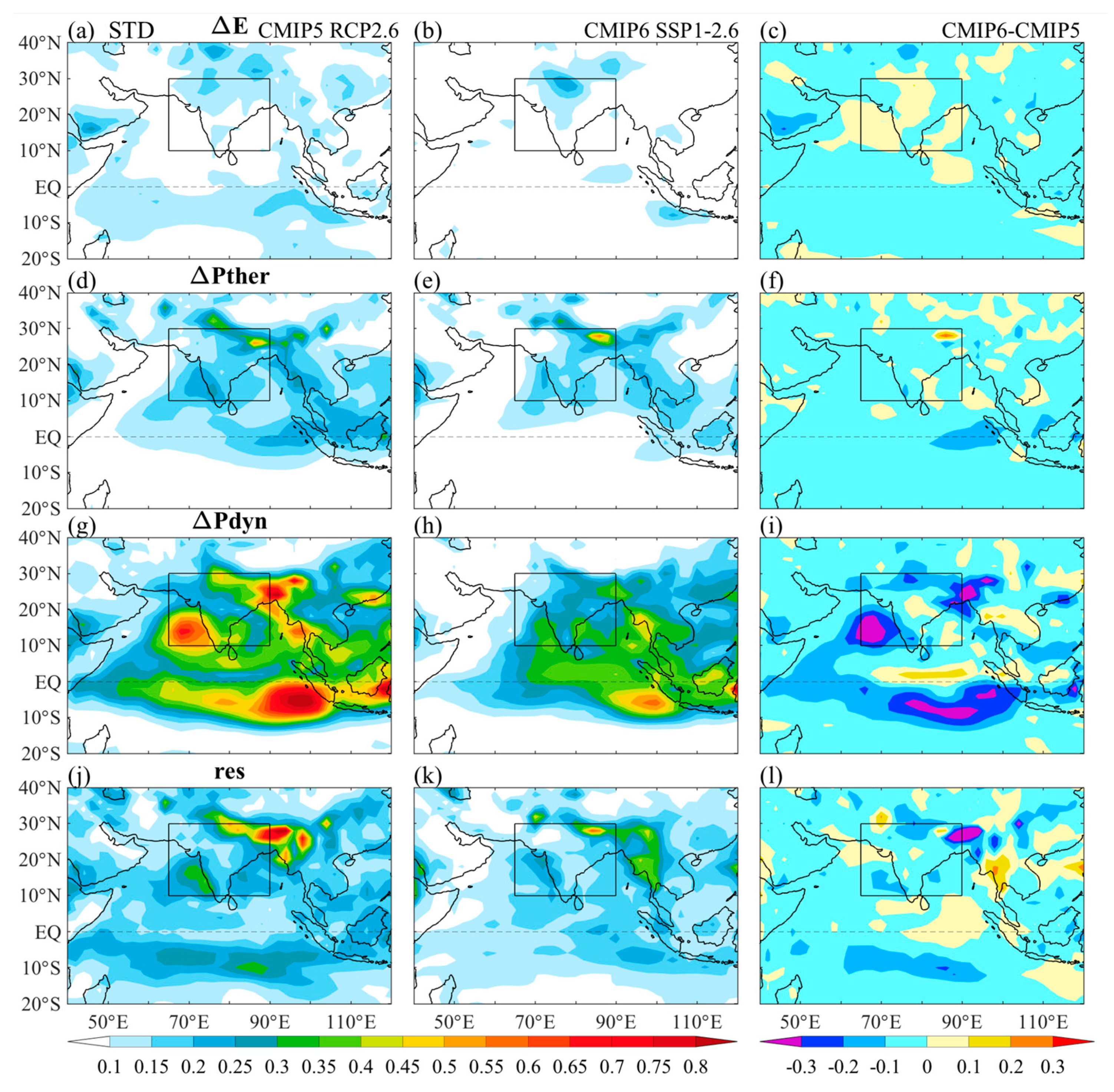
Figure 2 shows the normalized MME JJAS precipitation change under RCP2.6 in CMIP5 and SSP1-2.6 in CMIP6. Consistent with previous results under high-emission scenarios [3,35], a wetter ISM is projected in both RCP2.6 and SSP1-2.6 scenarios (Figure 2a,b). Precipitation generally increases north of the equator and decreases in the eastern Indian Ocean south of the equator. Moisture budget analyses reveal that the wetter ISM is primarily contributed by the thermodynamical component (Figure 3d,e), with a minor contribution from the enhanced local evaporation (Figure 3a,b). In contrast, the dynamical component suppresses the increase in ISM precipitation over most regions in RCP2.6 (Figure 3g), especially over the warm pool. The dominance of the thermodynamical component mainly results from the significantly increased atmospheric moisture in a warmer climate (Figure 4d,e), while the negative contribution from the dynamical component may indicate the slowdown of Walker circulation [7,48] and monsoon circulation under low-emission scenarios (Figure 4g,h).
However, the magnitude and spatial pattern of the ISM precipitation change differ between CMIP5 and CMIP6 models as well as the model consistency in the sign of precipitation change. For MME, the CMIP6 models display much larger precipitation increase and higher model consistency in the sign of change than CMIP5 models over ISM region (black box in Figure 2c). This striking difference is mainly caused by the distinct dynamical components (Figure 3g–i) but not thermodynamical components (Figure 3d–f). Specifically, the dynamical drying effect in CMIP5 turns into wetting effect in CMIP6 over the west India and is largely reduced in the east India. As the difference in the climatological water vapor is negligible (Figure 4j–l), the distinct dynamical components between two CMIPs can be further explained by the enhanced circulation or reduced circulation slowdown from CMIP5 models to CMIP6 models (Figure 4i).
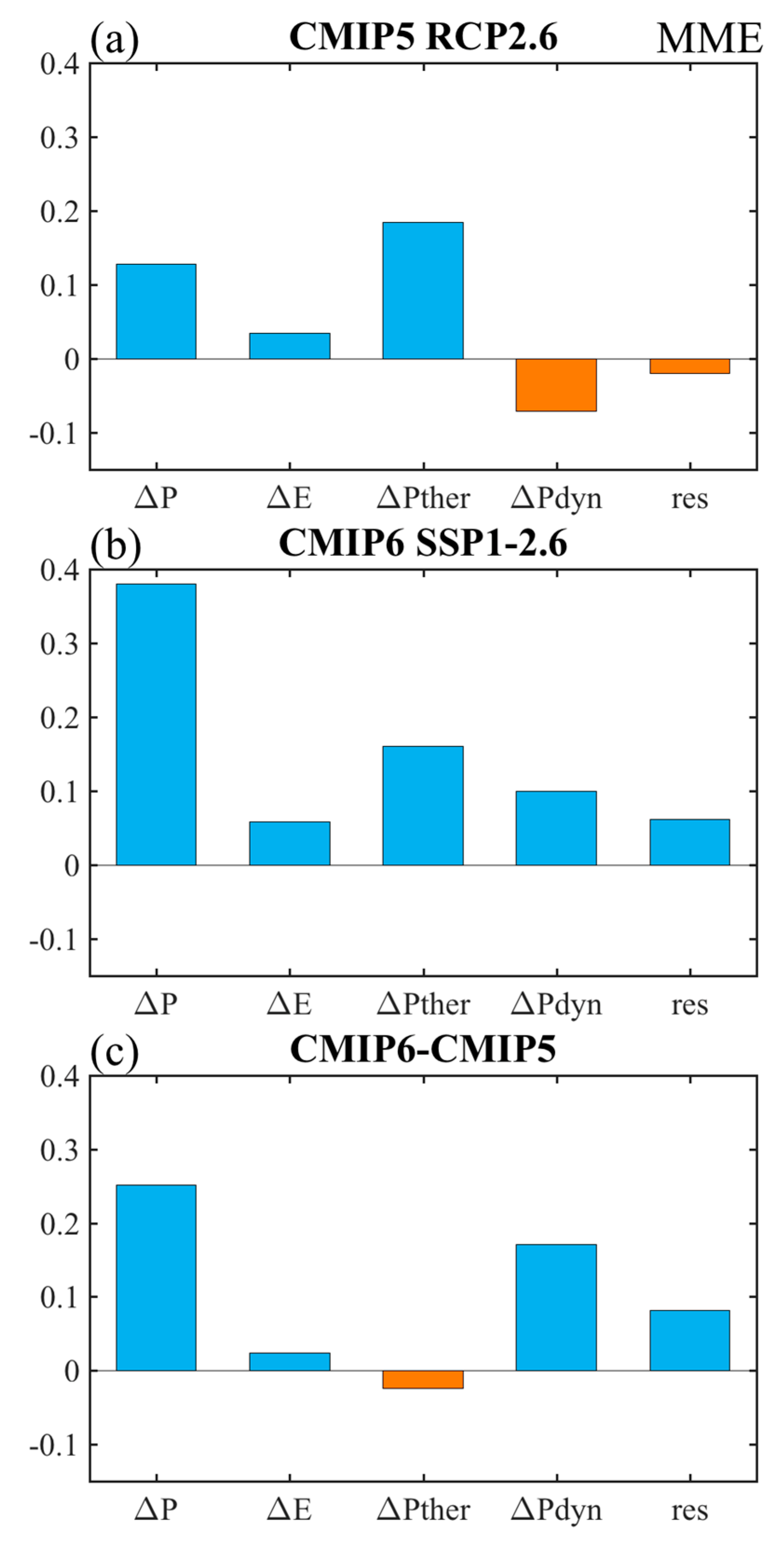
To quantify the relative role of each component on the ISM precipitation change, area-averaged precipitation change and its components over ISM region are further calculated (Figure 5). The area-weighted-mean results show that in both CMIP5 and CMIP6, the MME ISM precipitation increase is clearly dominated by the thermodynamical component (Figure 5a,b), with minor positive contribution from the enhanced local evaporation. However, the dynamical component dampens the ISM precipitation in CMIP5 but enhances it in CMIP6 (Figure 5c), which largely explains why the wetter ISM is much more pronounced in CMIP6 than CMIP5.
The ISM precipitation generally increases under both RCP2.6 and SSP1-2.6 but displays distinct spatial pattern and magnitude between CMIP5 and CMIP6 models. The similarity in the ISM precipitation change is mainly due to the high consistence in projecting the thermodynamical component in both CMIPs, while the differences in their magnitudes are primarily explained by the differences in the MME monsoon circulation change between CMIP5 and CMIP6. This calls for further in-depth investigation on what causes such distinct monsoon circulation change between two CMIPs but is not the focus of the present study.
4. Model Uncertainty in ISM Precipitation Change
In both CMIP5 and CMIP6, despite the fact that a wetter ISM is projected to occur (Figure 2), large spread in the sign and magnitude of ISM precipitation change may challenge the reliability of such projections, especially under low-emission scenarios where RF is much weaker than high-emission scenarios. It is of great importance to evaluate the uncertainty caused by the intermodel spread and trace its sources.
4.1. Sources of the Model Uncertainty
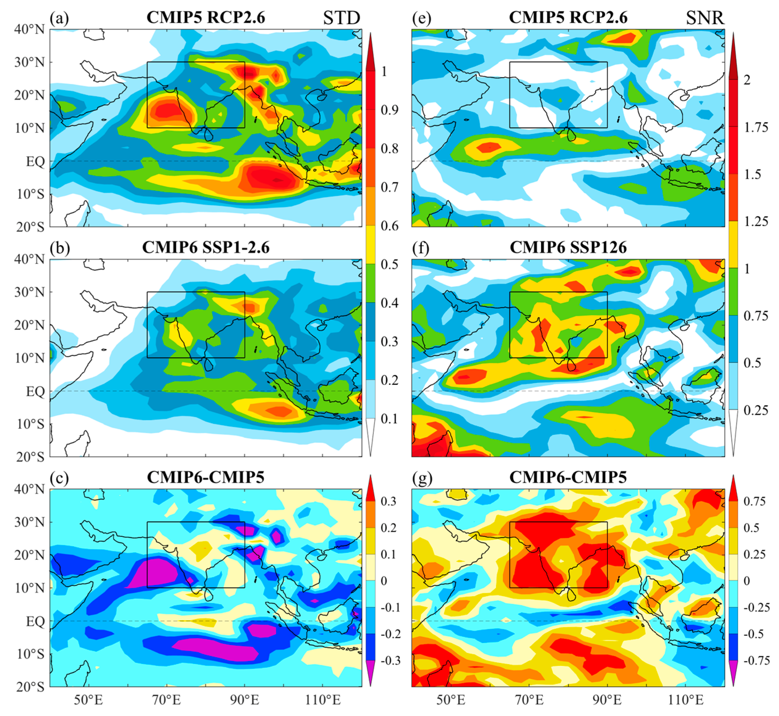
Figure 6 displays the magnitude of model uncertainty (i.e., intermodel standard deviation) and the SNR of ISM precipitation change under low-emission scenarios in CMIP5 and CMIP6. In both scenarios, precipitation uncertainty is large over the warm pool and South and East Asia (Figure 6a,b). In addition, the magnitude of the model uncertainty is prominently larger than the MME results in Figure 2, leaving the SNR to be well below 1 over most regions (Figure 6e,f). Low SNR suggests large inconsistency among models and hence low reliability in the climate models’ projections, casting doubt on the results that precipitation would increase in all ISM regions. This is distinct from the results under high-emission scenarios that the increase in ISM precipitation is relatively robust [3,35].
The magnitude of the model uncertainty in precipitation is clearly reduced over most IO and its surrounding regions and slightly enhanced over land regions and central equatorial IO in CMIP6 compared to CMIP5 (Figure 6c). As the MME precipitation change is much more enhanced in CMIP6 than CMIP5, the SNR significantly increases over most regions (Figure 6g), suggesting an increase in the model consistency of the precipitation projections. However, the enhanced SNR in CMIP6 stays at around 1 over most ISM region, indicating the MME results still remains highly uncertain. Figure 7 shows the intermodel STD of the components of precipitation change. The dynamical components stand out as the dominant source of uncertainty in ISM precipitation change under both RCP2.6 and SSP1-2.6 (Figure 7g,h), with relatively small contribution from other components. Besides, the overall reduced model uncertainty in ISM precipitation change is also mostly contributed by the dynamical component (Figure 7i), which is further related to the suppressed intermodel spread in ISM circulation change.
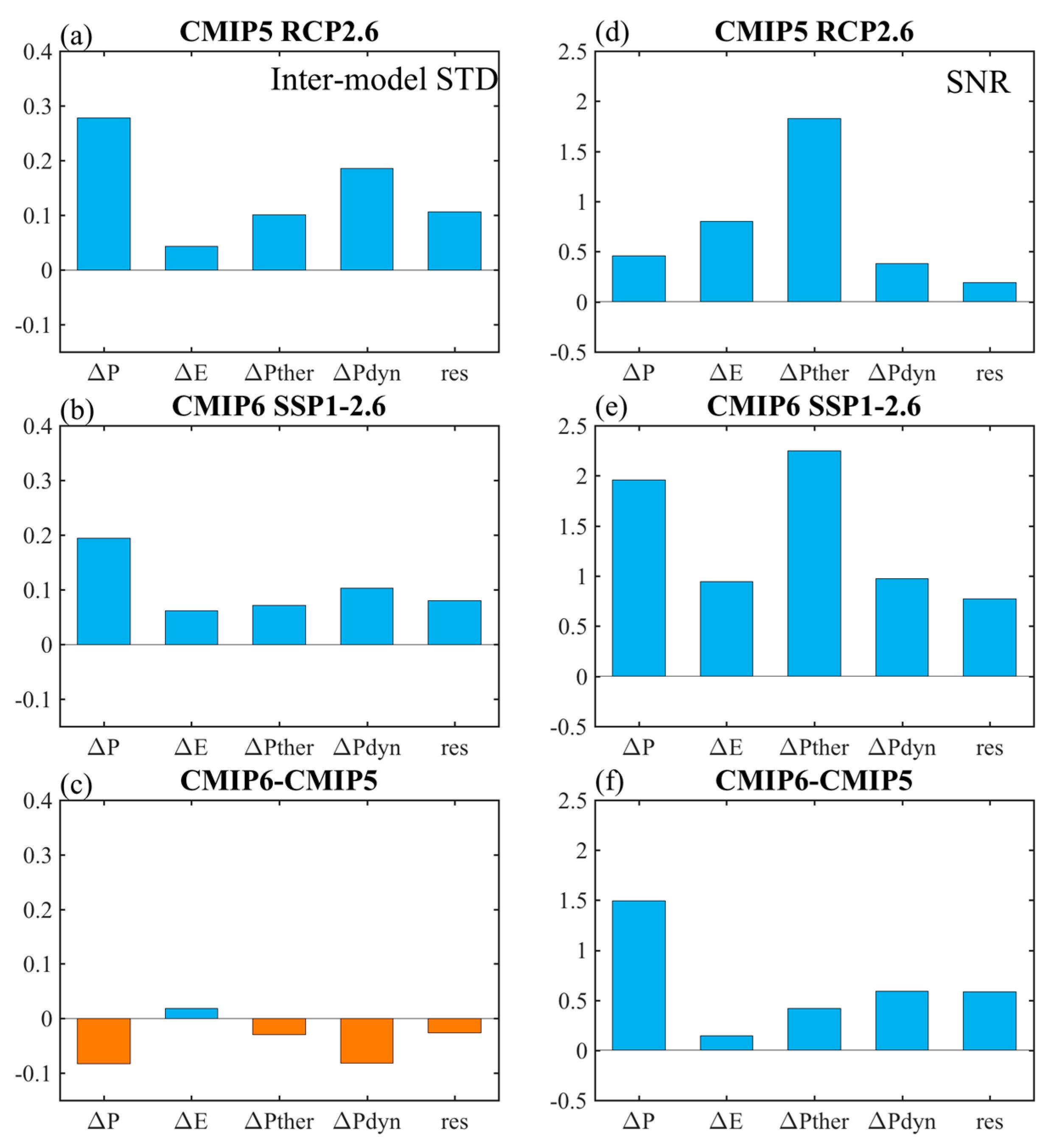
The above results are also confirmed by the uncertainty analyses for area-weighted-mean ISM precipitation change (Figure 8a,b). Under both RCP2.6 and SSP1-2.6, the intermodel STD of the dynamical component is around two times of that of the thermodynamical component. In addition, the uncertainty caused by the evaporation change is relatively small. From CMIP5 to CMIP6, the magnitude of intermodel STD reduces in ISM precipitation and all of its components except evaporation change (Figure 7c).
For SNR, the thermodynamical component displays the largest ratio, above 1.5 in RCP2.6 and 2 in SSP1-2.6 (Figure 8), suggesting relatively high model consistency in projecting the thermodynamical conditions for ISM precipitation increase. The SNR of other components is well below 1, even for evaporation change which displays the smallest magnitude of intermodel STD. It is worth noting that the SNR of ISM precipitation change significantly increases from 0.3 to 1.6 (Figure 8d,e), which is jointly contributed by the significantly enhanced precipitation increase (Figure 5) and reduced model uncertainty (Figure 8a,b) in CMIP6 than CMIP5. The MME thermodynamical component remains nearly the same but its model uncertainty is reduced from CMIP5 to CMIP6, causing increased SNR in thermodynamical component in CMIP6. The SNR of evaporation change is also slightly increased mainly due to enhanced evaporation from CMIP5 to CMIP6. For the dynamical component, its SNR slightly reduces from CMIP5 to CMIP6, mainly due to dynamical wetting in CMIP6 is smaller in magnitude than the dynamical drying effect in CMIP5.
4.2. Physical Processes for the Model Uncertainty
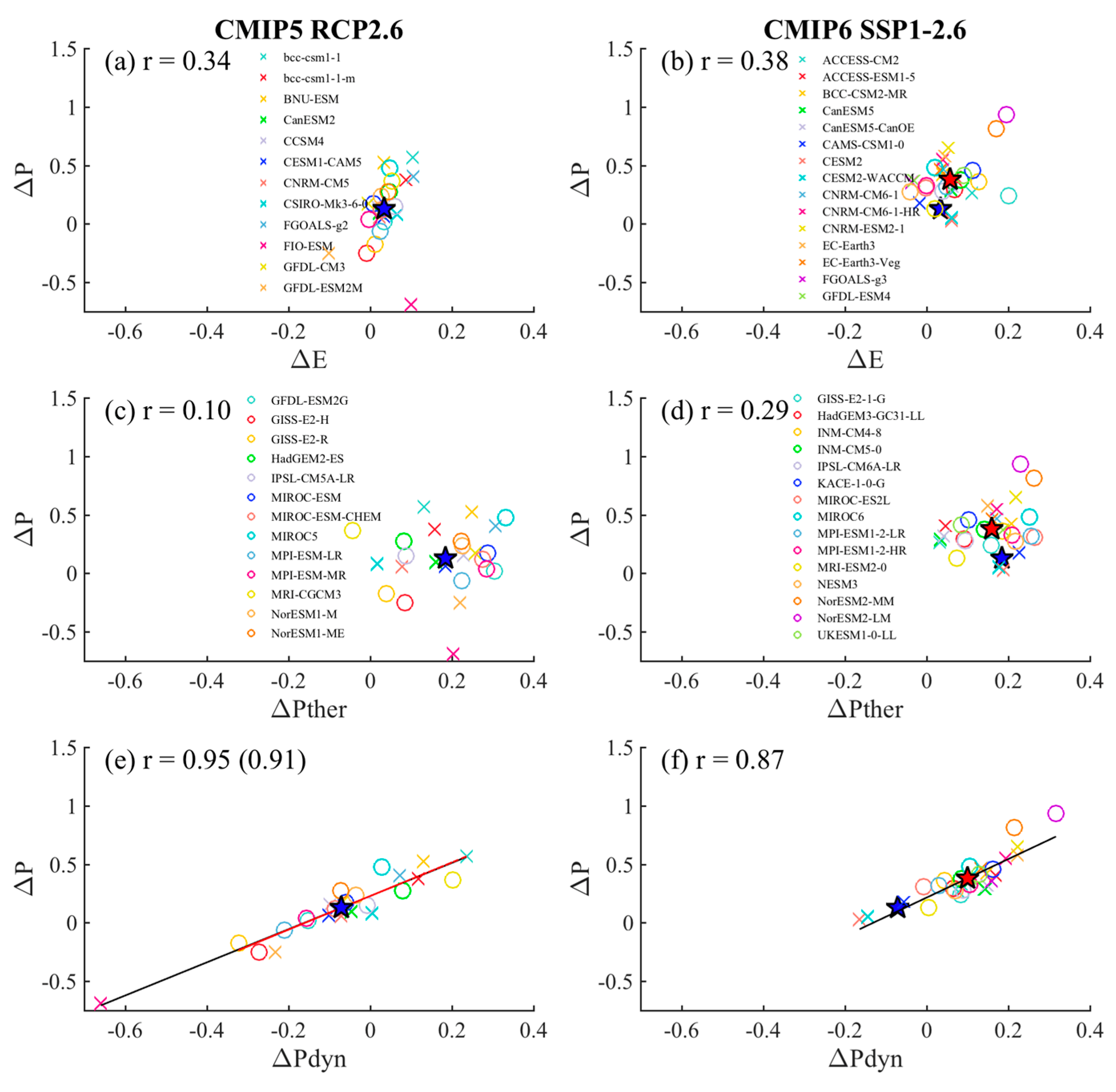
High model uncertainty indicates large intermodel spread but cannot explain what causes the spread across models. The intermodel correlation analyses can throw light on the relationship of relevant processes that may produce the model-to-model differences. Figure 9 shows the intermodel relationship between ISM precipitation change and its components in RCP2.6 and SSP1-2.6. The correlation coefficient is relatively low between precipitation change and evaporation change and thermodynamical component (Figure 9a–d), suggesting that them explain a small portion of the intermodel variance in ISM precipitation change. In contrast, the dynamical component displays a high correlation coefficient (above 0.85) with ISM precipitation change in both RCP2.6 and SSP1-2.6. Therefore, the intermodel differences in the dynamical component dominates the intermodel variance in ISM precipitation change. Moreover, the thermodynamical component (evaporation change) promotes ISM precipitation increase in all (most) models (Figure 9a–d), while the dynamical component strikingly differing in its sign across models (Figure 9e,f). In CMIP5, more than two thirds of models (19 out of 25) project that the dynamical component dampens the ISM precipitation. In contrast, the dynamical component promotes ISM precipitation in nearly two thirds of models (22 out of 30) in CMIP6. This leads to a reversion of the MME dynamical component from drying effect in CMIP5 to wetting effect in CMIP6 on MME ISM precipitation. Moreover, the intermodel spread in the dynamical component mainly follows that of the ISM circulation change, with intermodel correlations coefficients up to nearly 1 in both RCP2.6 and SSP1-2.6.
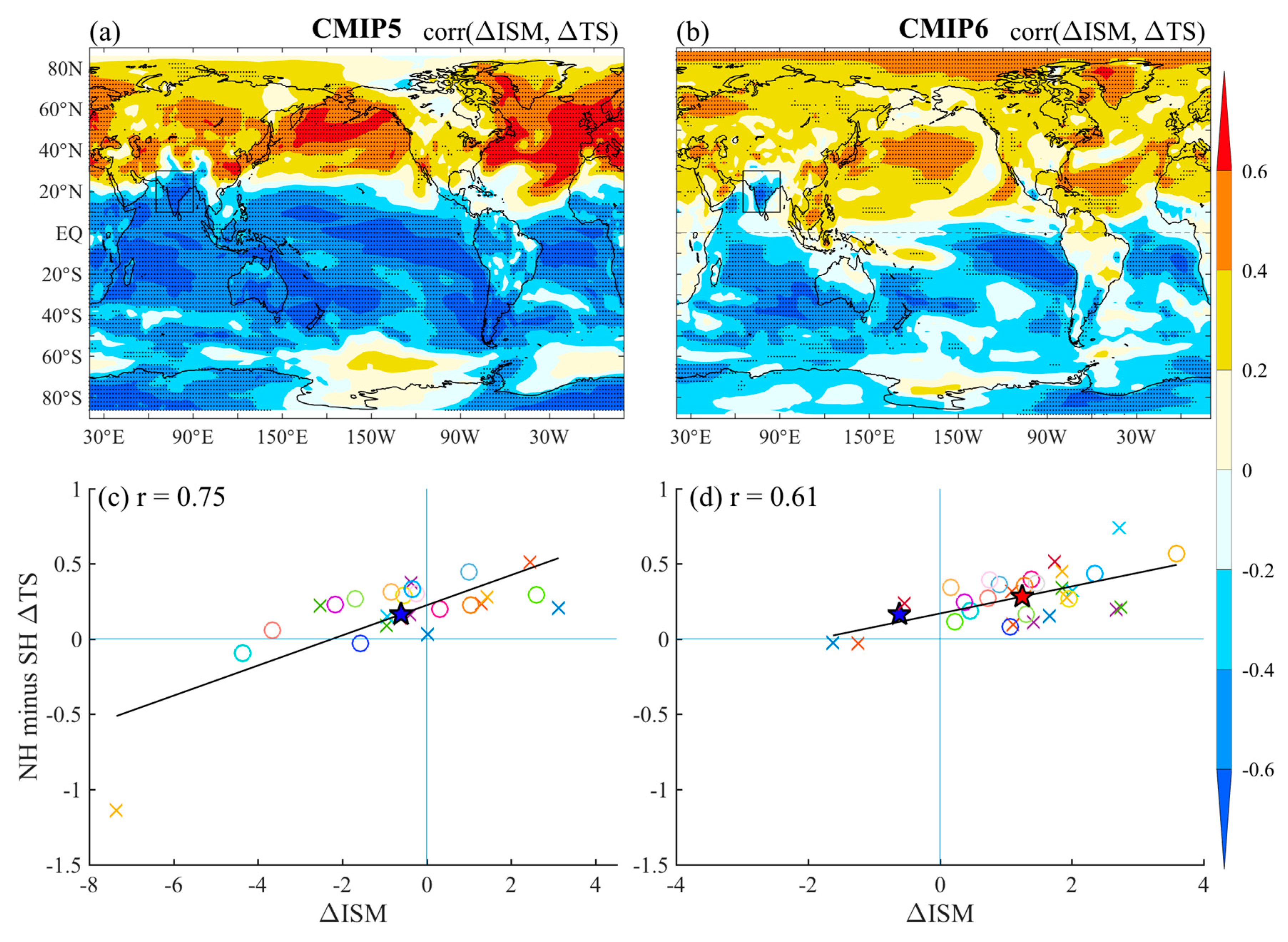
Furthermore, it is natural to ask what leads to the model-to-model differences in ISM response and why CMIP5 and CMIP6 models display distinct MME ISM circulation changes. Given that surface warming pattern is tightly coupled with atmospheric circulation change [7,28,29,48,49]. The ISM circulation change index, defined as area-weighted-mean over ISM regions, is thus correlated with surface temperature change among models at each grid (Figure 10a,b). The ISM circulation change generally positively correlates with surface temperature change in the Northern Hemisphere (NH) while negatively correlates with surface temperature change in the Southern Hemisphere (SH). Specifically, the positive (negative) intermodel correlation is prominent north (south) of 20° N in CMIP5 models at nearly all longitudes (Figure 10a). In CMIP6, this interhemispheric contrast in the correlation coefficient is much weaker than that in CMIP5 and the dividing line centers around 10° N (Figure 10b). Significant positive (negative) correlation appears over the North Pacific and Atlantic Oceans (SH subtropics) in CMIP6. Indeed, the interhemispheric surface warming contrast, defined as the differences in surface temperature change between 40° S–10° N and 10–60° N, is significantly correlated with the ISM circulation change among models (Figure 10c,d). The intermodel correlation coefficient between them is 0.75 in CMIP5 and 0.61 in CMIP6, suggesting that the interhemispheric surface warming contrast is important in explaining the intermodel variance in ISM circulation change.
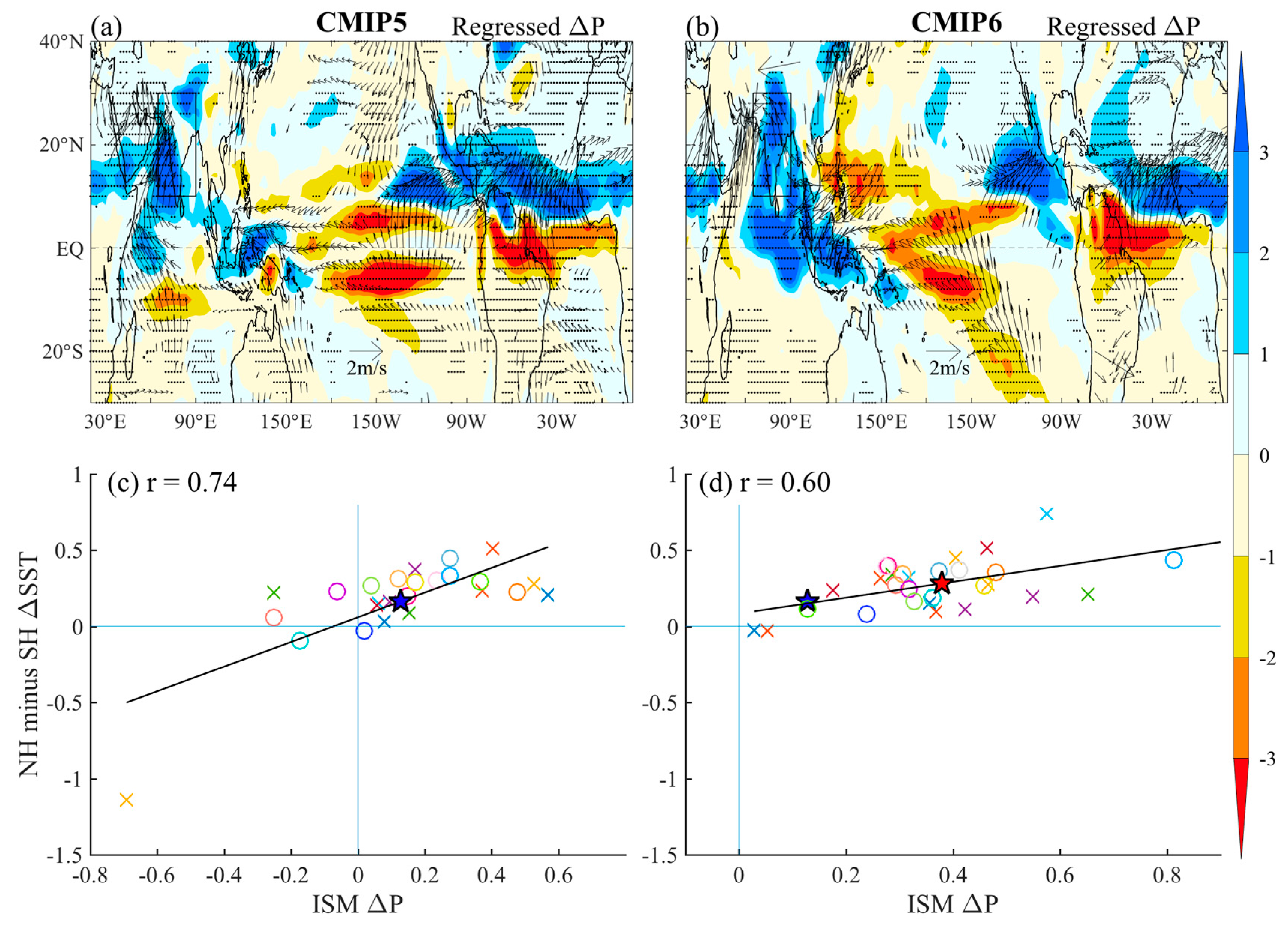
To further explore the underlying processes, the changes in precipitation and 925 hPa wind are regressed onto the interhemispheric surface warming index among models at each grid, all based on variables normalized by GMST rise at 2050–2099 referenced to 1900–1949 (Figure 11). In response to the interhemispheric warming contrast, there is strong cross-equatorial southerly wind in all three basins. As a result, the precipitation generally increases in the NH and decreases in the SH, especially between 20° S–30° N. In the IO, the cross-equatorial southerly wind increases the ISM circulation and hence ISM precipitation in both CMIPs. Therefore, models displaying a large NH minus SH warming contrast tend to project a wetter ISM and vice versa.
In particular, the regressed ISM precipitation increase over the Bay of Bengal and eastern IO is not presented in CMIP5 models. Indeed, the interhemispheric surface warming contrast is overall larger in CMIP6 than CMIP5 (Figure 11c,d). Besides, the anticyclonic wind response over the Northwestern Pacific also largely promotes the ISM circulation and hence precipitation in CMIP6 models. These two factors may jointly contribute to explain why the ISM circulation and precipitation are largely enhanced from CMIP5 to CMIP6 models. Following an increased NH-SH warming gradient in CMIP6 compared to CMIP5 (blue and red stars in Figure 11d), the ISM precipitation also increases significantly. This suggests that the distinct ISM circulation and precipitation change between CMIP5 and CMIP6 can be largely explained by the differences in interhemispheric warming contrast, which may be further related to the enhanced Arctic warming (Figure 10b), substantially different cloud simulation, deep convective schemes in CMIP6 compared to CMIP5 [46,47,50]. Indeed, the CMIP6 models is revealed to be more capable than CMIP5 models in reproducing the spatial and temporal pattern of ISM [16], this may also contribute to some extent.
5. Summary and Discussion
The ISM precipitation is vital for densely populated South Asian countries due to its enormous impacts on agriculture, freshwater availability, ecosystems and human health. Reliable future projections of ISM precipitation under global warming are of great importance for decision-making of adaptation policies to climate change for South Asian countries. Under high-emission scenarios, previous studies suggest that models consistently project a wetter ISM due to favorable conditions of increased moisture from enhanced surface warming [3,19]. However, large intermodel spread or model uncertainty lies in the climate models’ projections of precipitation change. Therefore, the model uncertainty in ISM precipitation change under low-emission scenarios in CMIP5 and CMIP6 is analyzed and its underlying mechanisms are investigated in the present study.
The results show that the MME ISM precipitation is still projected to increase under low-emission scenarios in both CMIP5 and CMIP6, similar to the results under high-emission scenarios. Moisture budget analyses show that the thermodynamical component due to moisture increases dominate the increase in ISM precipitation. However, the intermodel spread of the projected ISM precipitation change is tremendous. The SNR of precipitation change is still around 1 in most ISM regions. This casts doubts on a wetter ISM in a warmer climate under low-emission scenarios. Moreover, most of the model uncertainty in ISM precipitation change can be traced back to the intermodel differences in the dynamical component due to the atmospheric circulation change but not the thermodynamical component, different from the MME case. The present study further shows that the interhemispheric surface warming contrast is important in causing the intermodel differences in ISM circulation change and hence precipitation change. This is because models displaying large NH minus SH warming contrast tend to produce strong cross-equatorial southerly wind change that would intensify the meridional wind and, thus, promote ISM precipitation and vice versa. The importance of the interhemispheric temperature gradient change in regulating the spread in ISM circulation change across models is consistent with previous studies [51,52,53,54,55,56].
An important result is that the wetter ISM is clearly enhanced in CMIP6 compared to CMIP5, mainly due to the transition of the dynamical component from drying effect in CMIP5 to wetting effect in CMIP6. In addition, model uncertainty is significantly reduced from CMIP5 to CMIP6. As a result, the SNR of ISM precipitation strikingly increases in CMIP6. However, the SNR of precipitation change is still low over most ISM regions, suggesting highly uncertain ISM change under low-emission scenarios. This may due to the fact that natural variability would large disturb the climate change signal under weak anthropogenic RF. Therefore, despite that the model consistency is increased in CMIP6 compared to CMIP5, it is still unclear how the ISM will change when RF is relatively weak, such as under low warming scenarios or 1.5 °C and 2 °C low warming target. For decision makers, a highly uncertain ISM change implies that a drier ISM is also possible in the future, which would make it hard to make decisions in adaptation policies for South Asian countries. It also requires inspection and investment in infrastructures, water supplies, agriculture and human health to prepare for both a wetter and drier ISM conditions.
The present study also highlights that ISM precipitation change displays large differences between CMIP5 and CMIP6 models, which is also confirmed by results under high-emission scenarios [50]. The reasons causing the distinct ISM response between CMIP5 and CMIP6 models, especially the interhemispheric warming contrast, is worthy of further in-depth study. Indeed, the increased complexity model physics in CMIP6 compared to CMIP5 may not directly lead to increased model consistency and hence reduced uncertainty, because the improvement in one aspect of model may be incompatible with existing model physics and hence new errors in other aspects and hence increased uncertainty. Moreover, as the ISM circulation change involves complicated processes or factors, like the monsoon physics, cloud feedback, convection schemes and topography, the ISM circulation change may also display substantial spread across models even under the same surface warming pattern. This calls for systematical and in-depth investigations the underlying reasons of the distinct ISM response between two CMIPs in the future.
Author Contributions
Data curation, S.-M.L.; investigation, S.-M.L. and G.L.; methodology, S.-M.L. and G.L.; supervision, G. L.; writing – original draft, S.-M.L. and G.L.; Writing–review and editing, G.L. All authors have read and agreed to the published version of the manuscript.
Funding
This work is supported by the Natural Science Foundation of China (42076208, 41706026, 41831175), National Key Research and Development Program of China (2017YFA0604600), and the Fundamental Research Funds for the Central Universities (B210202135, B210201015).
Institutional Review Board Statement
Not applicable.
Informed Consent Statement
Not applicable.
Data Availability Statement
The dataset analyzed in this study are publicly available on http://pcmdi9.llnl.gov/.
Acknowledgments
The authors acknowledge the WCRP Working Group on Coupled Modeling, which is responsible for CMIP, and the climate modeling groups for producing and making available their model outputs. The authors also thank the anonymous reviewers for their constructive comments that lead to improvements in the manuscript.
Conflicts of Interest
The authors declare no conflict of interest.
References
- Turner, A.G.; Slingo, J.M. Uncertainties in future projections of extreme precipitation. Atmos. Sci. Lett. 2009, 10, 152–158. [Google Scholar] [CrossRef]
- Turner, A.G.; Annamalai, H. Climate change and the South Asian summer monsoon. Nat. Clim. Chang. 2012, 2, 587–595. [Google Scholar] [CrossRef]
- IPCC. Climate Change 2013: The Physical Science Basis; UK Cambridge Univ. Press: Cambridge, UK, 2013. [Google Scholar] [CrossRef]
- Chen, X.; Zhou, T. Distinct effects of global mean warming and regional sea surface warming pattern on projected uncertainty in the South Asian summer monsoon. Geophys. Res. Lett. 2015, 42, 9433–9439. [Google Scholar] [CrossRef]
- Long, S.-M.; Xie, S.-P. Intermodel variations in projected precipitation change over the North Atlantic: Sea surface temperature effect. Geophys. Res. Lett. 2015, 42, 4158–4165. [Google Scholar] [CrossRef] [Green Version]
- Xie, S.-P.; Deser, C.; Vecchi, G.A.; Collins, M.; Delworth, T.L.; Hall, A.; Hawkins, E.; Johnson, N.C.; Cassou, C.; Giannini, A.; et al. Towards predictive understanding of regional climate change. Nat. Clim. Chang. 2015, 5, 921–930. [Google Scholar] [CrossRef]
- Long, S.-M.; Xie, S.-P.; Liu, W. Uncertainty in tropical rainfall projections: Atmospheric circulation effect and the Ocean Coupling. J. Clim. 2016, 29, 2671–2687. [Google Scholar] [CrossRef]
- Zhou, S.; Huang, G.; Huang, P. Changes in the East Asian summer monsoon rainfall under global warming: Moisture budget decompositions and the sources of uncertainty. Clim. Dyn. 2018, 51, 1363–1373. [Google Scholar] [CrossRef]
- Sabeerali, C.T.; Rao, S.A.; Dhakate, A.R.; Salunke, K.; Goswami, B.N. Why ensemble mean projection of south Asian monsoon rainfall by CMIP5 models is not reliable? Clim. Dyn. 2015, 45, 161–174. [Google Scholar] [CrossRef]
- Giorgi, F.; Francisco, R. Evaluating uncertainties in the prediction of regional climate change. Geophys. Res. Lett. 2000, 27, 1295–1298. [Google Scholar] [CrossRef]
- Hawkins, E.; Sutton, R. The potential to narrow uncertainty in regional climate predictions. Bull. Am. Meteorol. Soc. 2009, 90, 1095–1107. [Google Scholar] [CrossRef] [Green Version]
- Hawkins, E.; Sutton, R. The potential to narrow uncertainty in projections of regional precipitation change. Clim. Dyn. 2011, 37, 407–418. [Google Scholar] [CrossRef]
- Rowell, D.P. Sources of uncertainty in future changes in local precipitation. Clim. Dyn. 2012, 39, 1929–1950. [Google Scholar] [CrossRef]
- Zhou, S.; Huang, G.; Huang, P. A bias-corrected projection for the changes in East Asian summer monsoon rainfall under global warming. Clim. Dyn. 2020, 54. [Google Scholar] [CrossRef]
- Deser, C.; Phillips, A.; Bourdette, V.; Teng, H. Uncertainty in climate change projections: The role of internal variability. Clim. Dyn. 2012, 38, 527–546. [Google Scholar] [CrossRef] [Green Version]
- Gusain, A.; Ghosh, S.; Karmakar, S. Added value of CMIP6 over CMIP5 models in simulating Indian summer monsoon rainfall. Atmos. Res. 2020, 232, 104680. [Google Scholar] [CrossRef]
- Long, S.-M.; Li, G.; Hu, K.; Ying, J. Origins of the IOD-like Biases in CMIP Multimodel Ensembles: The Atmospheric Component and Ocean–Atmosphere Coupling. J. Clim. 2020, 33, 10437–10453. [Google Scholar] [CrossRef]
- Kripalani, R.H.; Oh, J.H.; Kulkarni, A.; Sabade, S.S.; Chaudhari, H.S. South Asian summer monsoon precipitation variability: Coupled climate model simulations and projections under IPCC AR4. Theor. Appl. Climatol. 2007. [Google Scholar] [CrossRef]
- Li, G.; Xie, S.-P.; Du, Y. Monsoon-induced biases of climate models over the tropical Indian Ocean. J. Clim. 2015, 28, 3058–3072. [Google Scholar] [CrossRef] [Green Version]
- Li, G.; Xie, S.-P.; Du, Y. Climate model errors over the South Indian Ocean thermocline dome and their effect on the basin mode of interannual variability. J. Clim. 2015, 28, 3093–3098. [Google Scholar] [CrossRef] [Green Version]
- Li, G.; Xie, S.-P.; Du, Y. A robust but spurious pattern of climate change in model projections over the tropical Indian Ocean. J. Clim. 2016, 29, 5589–5608. [Google Scholar] [CrossRef] [Green Version]
- Wang, Z.; Li, G.; Yang, S. Origin of Indian summer monsoon rainfall biases in CMIP5 multimodel ensemble. Clim. Dyn. 2018, 51, 755–768. [Google Scholar] [CrossRef]
- Yang, B.; Zhang, Y.; Qian, Y.; Song, F.; Leung, L.R.; Wu, P.; Guo, Z.; Lu, Y.; Huang, A. Better monsoon precipitation in coupled climate models due to bias compensation. NPJ Clim. Atmos. Sci. 2019, 2, 1–8. [Google Scholar] [CrossRef]
- Annamalai, H.; Hamilton, K.; Sperber, K.R. The South Asian summer monsoon and its relationship with ENSO in the IPCC AR4 simulations. J. Clim. 2007, 20, 1071–1092. [Google Scholar] [CrossRef]
- Yang, B.; Zhang, Y.; Qian, Y.; Wu, T.; Huang, A.; Fang, Y. Parametric sensitivity analysis for the Asian summer monsoon precipitation simulation in the Beijing Climate Center AGCM, version 2.1. J. Clim. 2015, 28, 5622–5644. [Google Scholar] [CrossRef]
- Seager, R.; Naik, N.; Vecchi, G.A. Thermodynamic and dynamic mechanisms for large-scale changes in the hydrological cycle in response to global warming. J. Clim. 2010, 23, 4651–4668. [Google Scholar] [CrossRef] [Green Version]
- Held, I.M.; Soden, B.J. Robust responses of the hydrological cycle to global warming. J. Clim. 2006, 19, 5686–5699. [Google Scholar] [CrossRef]
- Chadwick, R.; Boutle, I.; Martin, G. Spatial patterns of precipitation change in CMIP5: Why the rich do not get richer in the tropics. J. Clim. 2013, 26, 3803–3822. [Google Scholar] [CrossRef]
- Huang, P.; Xie, S.-P.; Hu, K.; Huang, G.; Huang, R. Patterns of the seasonal response of tropical rainfall to global warming. Nat. Geosci. 2013, 6, 357–361. [Google Scholar] [CrossRef]
- May, W. Simulated changes of the Indian summer monsoon under enhanced greenhouse gas conditions in a global time-slice experiment. Geophys. Res. Lett. 2002, 29, 1118. [Google Scholar] [CrossRef] [Green Version]
- Cherchi, A.; Alessandri, A.; Masina, S.; Navarra, A. Effects of increased CO2 levels on monsoons. Clim. Dyn. 2011, 37, 83–101. [Google Scholar] [CrossRef] [Green Version]
- Endo, H.; Kitoh, A. Thermodynamic and dynamic effects on regional monsoon rainfall changes in a warmer climate. Geophys. Res. Lett. 2014, 41, 1704–1710. [Google Scholar] [CrossRef]
- Ueda, H.; Iwai, A.; Kuwako, K.; Hori, M.E. Impact of anthropogenic forcing on the Asian summer monsoon as simulated by eight GCMs. Geophys. Res. Lett. 2006, 33, L06703. [Google Scholar] [CrossRef]
- May, W. The sensitivity of the Indian summer monsoon to a global warming of 2°C with respect to pre-industrial times. Clim. Dyn. 2011, 37, 1843–1868. [Google Scholar] [CrossRef]
- Li, G.; Xie, S.-P.; He, C.; Chen, Z. Western Pacific emergent constraint lowers projected increase in Indian summer monsoon rainfall. Nat. Clim. Chang. 2017, 7, 708–712. [Google Scholar] [CrossRef]
- IPCC. Special Report on Global Warming of 1.5°C; UK Cambridge Univ. Press: Cambridge, UK, 2018. [Google Scholar] [CrossRef] [Green Version]
- Palter, J.B.; Frölicher, T.L.; Paynter, D.; John, J.G. Climate, ocean circulation, and sea level changes under stabilization and overshoot pathways to 1.5K warming. Earth Syst. Dyn. 2018, 9, 817–828. [Google Scholar] [CrossRef] [Green Version]
- Qu, X.; Huang, G. Different multi-year mean temperature in mid-summer of South China under different 1.5 °C warming scenarios. Sci. Rep. 2018, 8, 2–8. [Google Scholar] [CrossRef] [PubMed]
- Zhang, W.; Zhou, T.; Zou, L.; Zhang, L.; Chen, X. Reduced exposure to extreme precipitation from 0.5 °C less warming in global land monsoon regions. Nat. Commun. 2018, 9, 3153. [Google Scholar] [CrossRef] [Green Version]
- Chen, L.; Qu, X.; Huang, G.; Gong, Y. Projections of East Asian summer monsoon under 1.5 °C and 2 °C warming goals. Theor. Appl. Climatol. 2019, 137, 2187–2201. [Google Scholar] [CrossRef]
- Long, S.-M.; Xie, S.-P.; Du, Y.; Liu, Q.; Zheng, X.-T.; Huang, G.; Hu, K.M.; Ying, J. Effects of Ocean Slow Response under Low Warming Targets. J. Clim. 2020, 33, 477–496. [Google Scholar] [CrossRef]
- van Vuuren, D.P.; Edmonds, J.; Kainuma, M.; Riahi, K.; Thomson, A.; Hibbard, K.; Hurtt, G.C.; Kram, T.; Krey, V.; Jean-Francois Lamarque, J.-F.; et al. The representative concentration pathways: An overview. Clim. Chang. 2011, 109, 5–31. [Google Scholar] [CrossRef]
- Sanderson, B.M.; O’Neill, B.C.; Tebaldi, C. What would it take to achieve the Paris temperature targets? Geophys. Res. Lett. 2016, 43, 7133–7142. [Google Scholar] [CrossRef]
- Xu, Y.; Ramanathan, V. Well below 2 °C: Mitigation strategies for avoiding dangerous to catastrophic climate changes. Proc. Natl. Acad. Sci. USA 2017, 114, 10315–10323. [Google Scholar] [CrossRef] [PubMed] [Green Version]
- Taylor, K.E.; Stouffer, R.J.; Meehl, G.A. An overview of CMIP5 and the experiment design. Bull. Am. Meteorol. Soc. 2012, 35, 485–498. [Google Scholar] [CrossRef] [Green Version]
- Eyring, V.; Bony, S.; Meehl, G.A.; Senior, C.A.; Stevens, B.; Stouffer, R.J.; Taylor, K.E. Overview of the Coupled Model Intercomparison Project Phase 6 (CMIP6) experimental design and organization. Geosci. Model Dev. 2016, 9, 1937–1958. [Google Scholar] [CrossRef] [Green Version]
- Zelinka, M.D.; Myers, T.A.; McCoy, D.T.; Po-Chedley, S.; Caldwell, P.M.; Ceppi, P.; Stephen, A.K.; Karl, E.T. Causes of higher climate sensitivity in CMIP6 models. Geophys. Res. Lett. 2020, 47, e2019GL085782. [Google Scholar] [CrossRef] [Green Version]
- Ma, J.; Xie, S.-P.; Kosaka, Y. Mechanisms for tropical tropospheric circulation change in response to global warming. J. Clim. 2012, 25, 2979–2994. [Google Scholar] [CrossRef]
- Xie, S.-P.; Deser, C.; Vecchi, G.A.; Ma, J.; Teng, H.; Wittenberg, A.T. Global warming pattern formation: Sea surface temperature and rainfall. J. Clim. 2010, 23, 966–986. [Google Scholar] [CrossRef]
- Katzenberger, A.; Schewe, J.; Pongratz, J.; Levermann, A. Robust increase of Indian monsoon rainfall and its variability under future warming in CMIP-6 models. Earth Syst. Dyn. 2020. [Google Scholar] [CrossRef]
- Ramanathan, V.; Chung, C.; Kim, D.; Bettge, T.; Buja, L.; Kiehl, J.T.; Washington, W.M.; Fu, Q.; Sikka, D.R.; Wild, M. Atmospheric brown clouds: Impacts on South Asian climate and hydrologic cycle. Proc. Natl Acad. Sci. USA 2005, 102, 5326–5333. [Google Scholar] [CrossRef] [Green Version]
- Lau, K.-M.; Kim, K.-M. Observational relationships between aerosol and Asian monsoon rainfall, and circulation. Geophys. Res. Lett. 2006, 33, L21810. [Google Scholar] [CrossRef]
- Chung, C.; Ramanathan, V. Relationship between trends in land precipitation and tropical SST gradient. Geophys. Res. Lett. 2007, 34. [Google Scholar] [CrossRef]
- Roxy, M.K.; Ritika, K.; Terray, P.; Murtugudde, R.; Ashok, K.; Goswami, B.N. Drying of Indian subcontinent by rapid Indian Ocean warming and a weakening land-sea thermal gradient. Nat. Commun. 2015, 6, 7423. [Google Scholar] [CrossRef] [PubMed] [Green Version]
- Wu, G.; He, B.; Bao, Q.; Duan, A.; Jin, F.F. Thermal controls on the Asian summer monsoon. Sci. Rep. 2012, 2, 404. [Google Scholar] [CrossRef] [PubMed] [Green Version]
- Lau, K.-M.; Kim, K.-M.; Leuna, R. Changing circulation structure and precipitation characteristics in Asian monsoon regions: Greenhouse warming vs. aerosol effects. Geosci. Lett. 2017, 4, 28. [Google Scholar] [CrossRef] [PubMed]
Figure 1.
Global-mean annual-mean surface temperature change (°C) relative to preindustrial level (1850–1899 mean) in each model (colored thin lines) and its multi-model ensemble mean (MME) results (colored thick lines) in (a) CMIP5 and (b) CMIP6. The black thick lines indicate the radiative forcing (RF, W m−2) pathway, and the red dotted lines indicate the time of year 2050.

Figure 2.
Normalized multi-model ensemble mean (MME) ISM precipitation change (JJAS ∆Pn, mm day-1) (a) under RCP2.6 in CMIP5, (b) under SSP1-2.6 in CMIP6 and (c) their difference. The black cross indicates at least 2/3 models show the same sign with MME results. The domain for calculating area-mean ISM precipitation is 65–90° E and 10–30° N, indicating by the black box.

Figure 3.
Subcomponents of MME ISM precipitation change (mm day−1): (a–c) evaporation change (, mm day−1), (d–f) thermodynamical component (, mm day−1), (g–i) dynamical component (, mm day−1) and (j–l) residual term (, mm day−1) under RCP2.6 in CMIP5 and SSP1-2.6 in CMIP6 and their differences.
Figure 3.
Subcomponents of MME ISM precipitation change (mm day−1): (a–c) evaporation change (, mm day−1), (d–f) thermodynamical component (, mm day−1), (g–i) dynamical component (, mm day−1) and (j–l) residual term (, mm day−1) under RCP2.6 in CMIP5 and SSP1-2.6 in CMIP6 and their differences.

Figure 4.
June–July–August–September (JJAS) mean (a–c) climatological vertical velocity at 500 hPa (clim , positively upward, hPa day−1), (d–f) water vapor change (, g kg−1), (g–i) vertical velocity change at 500 hPa (, hPa day−1) and (j–l) climatological water vapor (, g kg−1) under RCP2.6 in CMIP5 and SSP1-2.6 in CMIP6 and their differences.

Figure 5.
Histograms for area-weighted-mean (65–90° E and 10–30° N, regions indicated by the black boxes in Figure 2, Figure 3 and Figure 4) MME ISM precipitation (mm day−1) and its subcomponents under (a) RCP2.6 and (b) SSP1-2.6 and (c) their differences.

Figure 6.
Intermodel standard deviation (STD, mm day−1) of precipitation change under (a) RCP2.6 and (b) SSP1-2.6 and (c) their differences. Signal-to-Noise ratio (SNR) of the MME precipitation change under (e) RCP2.6 and (f) SSP1-2.6 and (g) their differences.
Figure 6.
Intermodel standard deviation (STD, mm day−1) of precipitation change under (a) RCP2.6 and (b) SSP1-2.6 and (c) their differences. Signal-to-Noise ratio (SNR) of the MME precipitation change under (e) RCP2.6 and (f) SSP1-2.6 and (g) their differences.

Figure 7.
Intermodel standard deviation (STD, mm day−1) for the subcomponents of precipitation change under (a,d,g,j) RCP2.6 and (b,e,h,k) SSP1-2.6 and (c,f,i,l) their differences.
Figure 7.
Intermodel standard deviation (STD, mm day−1) for the subcomponents of precipitation change under (a,d,g,j) RCP2.6 and (b,e,h,k) SSP1-2.6 and (c,f,i,l) their differences.

Figure 8.
Histograms of (a–c) intermodel standard deviation (STD, mm day−1) and (d–f) Signal-to-Noise ratio (SNR) for area-weighted-mean (65–90° E and 10–30° N) MME ISM precipitation (mm day−1) and its subcomponents under RCP2.6 and SSP1-2.6 and their differences.
Figure 8.
Histograms of (a–c) intermodel standard deviation (STD, mm day−1) and (d–f) Signal-to-Noise ratio (SNR) for area-weighted-mean (65–90° E and 10–30° N) MME ISM precipitation (mm day−1) and its subcomponents under RCP2.6 and SSP1-2.6 and their differences.

Figure 9.
Scatterplot of intermodel relationship between ISM precipitation change and (a–b) evaporation change (, mm day−1), (c–d) thermodynamical component (, mm day−1) and (e–f) dynamical component (, mm day−1). The blue and red stars, respectively, indicate the CMIP5 and CMIP6 MME results. The least squares fitting lines are shown on panels where the intermodel correlation is significant at 95% confidence level. The red fitting line and correlation coefficient in the bracket in Figure 9e are based on the analyses excluding the outlier at the bottom-left corner.

Figure 10.
Spatial pattern of intermodel correlation coefficients between area-weighted-mean ISM circulation change () and surface temperature change () in (a) CMIP5 and (b) CMIP6. (c) and (d) are the scatterplots of and Northern Hemisphere (NH) minus Southern Hemisphere (SH) surface warming contrast among models. The black dots indicate the correlation coefficients significate at 95% confidence level. The blue and red stars, respectively, indicate the CMIP5 and CMIP6 MME results.

Figure 11.
Spatial pattern of regressed precipitation change (, shading, hPa/day) and 925 hPa winds (vectors, m s−1) onto the NH minus SH surface warming contrast indices among models in (a) CMIP5 and (b) CMIP6. Note that only zonal or meridional winds significate at 90% confidence level are plotted. (c) and (d) are the scatterplots between ISM and NH minus SH surface warming contrast among models. The blue and red stars, respectively, indicate the CMIP5 and CMIP6 MME results.


Table 1.
A list of the models used in the present study.
| CMIP5 (25) | CMIP6 (30) | ||||||
|---|---|---|---|---|---|---|---|
| 1 | bcc-csm1-1-m | 16 | HadGEM2-ES | 1 | ACCESS-CM2 | 16 | GISS-E2-1-G |
| 2 | bcc-csm1-1 | 17 | IPSL-CM5A-LR | 2 | ACCESS-ESM1-5 | 17 | HadGEM3-GC31-LL |
| 3 | BNU-ESM | 18 | MIROC-ESM | 3 | BCC-CSM2-MR | 18 | INM-CM4-8 |
| 4 | CanESM2 | 19 | MIROC-ESM-CHEM | 4 | CanESM5 | 19 | INM-CM5-0 |
| 5 | CCSM4 | 20 | MIROC5 | 5 | CanESM5-CanOE | 20 | IPSL-CM6A-LR |
| 6 | CESM1-CAM5 | 21 | MPI-ESM-LR | 6 | CAMS-CSM1-0 | 21 | KACE-1-0-G |
| 7 | CNRM-CM5 | 22 | MPI-ESM-MR | 7 | CESM2 | 22 | MIROC-ES2L |
| 8 | CSIRO-Mk3-6-0 | 23 | MRI-CGCM3 | 8 | CESM2-WACCM | 23 | MIROC6 |
| 9 | FGOALS-g2 | 24 | NorESM1-M | 9 | CNRM-CM6-1 | 24 | MPI-ESM1-2-LR |
| 10 | FIO-ESM | 25 | NorESM1-ME | 10 | CNRM-CM6-1-HR | 25 | MPI-ESM1-2-HR |
| 11 | GFDL-CM3 | 11 | CNRM-ESM2-1 | 26 | MRI-ESM2-0 | ||
| 12 | GFDL-ESM2M | 12 | EC-Earth3 | 27 | NESM3 | ||
| 13 | GFDL-ESM2G | 13 | EC-Earth3-Veg | 28 | NorESM2-MM | ||
| 14 | GISS-E2-H | 14 | FGOALS-g3 | 29 | NorESM2-LM | ||
| 15 | GISS-E2-R | 15 | GFDL-ESM4 | 30 | UKESM1-0-LL | ||
Publisher’s Note: MDPI stays neutral with regard to jurisdictional claims in published maps and institutional affiliations. |
© 2021 by the authors. Licensee MDPI, Basel, Switzerland. This article is an open access article distributed under the terms and conditions of the Creative Commons Attribution (CC BY) license (http://creativecommons.org/licenses/by/4.0/).
Share and Cite
MDPI and ACS Style
Long, S.-M.; Li, G. Model Uncertainty in the Projected Indian Summer Monsoon Precipitation Change under Low-Emission Scenarios. Atmosphere 2021, 12, 248. https://0-doi-org.brum.beds.ac.uk/10.3390/atmos12020248
AMA Style
Long S-M, Li G. Model Uncertainty in the Projected Indian Summer Monsoon Precipitation Change under Low-Emission Scenarios. Atmosphere. 2021; 12(2):248. https://0-doi-org.brum.beds.ac.uk/10.3390/atmos12020248
Chicago/Turabian StyleLong, Shang-Min, and Gen Li. 2021. "Model Uncertainty in the Projected Indian Summer Monsoon Precipitation Change under Low-Emission Scenarios" Atmosphere 12, no. 2: 248. https://0-doi-org.brum.beds.ac.uk/10.3390/atmos12020248
Note that from the first issue of 2016, this journal uses article numbers instead of page numbers. See further details here.