
Measuring Hydrogen in Indoor Air with a Selective Metal Oxide Semiconductor Sensor


Lab for Measurement Technology, Saarland University, Campus A5 1, 66123 Saarbruecken, Germany
*
Author to whom correspondence should be addressed.
Atmosphere 2021, 12(3), 366; https://0-doi-org.brum.beds.ac.uk/10.3390/atmos12030366
Submission received: 6 February 2021
/
Revised: 1 March 2021
/
Accepted: 5 March 2021
/
Published: 11 March 2021
(This article belongs to the Special Issue Indoor Air Quality—What Is Known and What Needs to Be Done)
Abstract
:Hydrogen is a ubiquitous but often neglected gas. In analytical measurements hydrogen—as a harmless gas—often is not considered so no studies on hydrogen in indoor air can be found. For metal oxide semiconductor (MOS) gas sensors that are increasingly pushed into the application as TVOC (total volatile organic compounds) sensors, hydrogen is a severe disturbance. On the other hand, hydrogen can be an intentional choice as indicator for human presence similar to carbon dioxide. We present a field-study on hydrogen in indoor air using selective MOS sensors accompanied by an analytical reference device for hydrogen with an accuracy of 10 ppb. Selectivity is achieved by siloxane treatment combined with temperature cycled operation and training with a complex lab calibration using randomized gas mixtures, yielding an uncertainty of 40–60 ppb. The feasibility is demonstrated by release tests with several gases inside a room and by comparison to the reference device. The results show that selective MOS sensors can function as cheap and available hydrogen detectors. Fluctuations in hydrogen concentration without human presence are measured over several days to gain insight in this highly relevant parameter for indoor air quality. The results indicate that the topic needs further attention and that the usage of hydrogen as indicator for human presence might be precluded by other sources and fluctuations.
1. Introduction
Indoor air quality (IAQ) is a general term comprising a multitude of parameters like temperature, humidity, air flow or the concentration of many trace gases [1]. The term is known since 1970 and of increasing interest during the last decades [2]. Among these trace gases are specific harmful pollutants like nitrogen dioxide (NO2); formaldehyde or benzene [3,4]; carbon dioxide (CO2), which is often used as indicator for human presence [5,6]; many organic compounds, often simply referred to as VOCs (volatile organic compounds) [7]; and others. Despite this high complexity inexpensive sensors are wanted for the purpose of IAQ monitoring. Nondispersive infrared sensors (NDIR) for CO2 monitoring are state of the art for demand-controlled ventilation if concentrations are above 1000 ppm, although this level is not harmful: Pettenkofer, who introduced this guideline value, already stated in 1858 that CO2 is only an indicator for other harmful and smelly organic substances emitted by human beings [5] and recent results from aerospace research support this assessment [8]. In today’s world VOCs are not only emitted by humans but also from other sources like furniture, personal care products or cleaning agents, so this approach of indirect VOC measurement might be erroneous [9].
Up-and-coming for real-time and direct VOC measurements are metal oxide semiconductor (MOS) gas sensors, which can already be found in many available IAQ monitors. These sensors show high sensitivity towards a wide range of reducing gases. Their selectivity—e.g., to a group of gases like VOCs—can be optimized by cyclically changing the temperature of the sensing layer (TCO, temperature cycled operation) [10,11]. This type of operation has been known for a long time [12], but is still often only used in research. Commercially available devices are typically operated at constant temperature yielding a simple sum signal for reducing gases.
Another trace gas that is not directly linked to IAQ, because it does not have a specific health effect, is hydrogen (H2), which can be found in the atmosphere at a concentration of 500 ppb [13]. MOS sensors are very sensitive to this gas especially at higher operating temperatures, where the sensors are generally operated. Since H2 in this concentration range (500 ppb and above) is not covered by typical analytical measurement techniques in gas measurement science (gas chromatography, sorption tubes, mass spectrometry, infrared spectrometry, photoionization detectors, etc.) little is known on the presence and dynamic of this gas in indoor air. For outdoor and atmospheric concentrations some studies can be found, indicating that H2 is a product of chemical industry and emitted from cars and other traffic [14], but also from the photochemical oxidation of methane (CH4) and VOCs [15,16]. An annual cycle with an amplitude of approximately 40 ppb and a diurnal cycle with an amplitude of approximately 3 ppb can be observed [14,15]. Therefore, even in outdoor air significant variations of the H2 concentration are expected in industrial and residential areas [17] and therefore also some variations are likely in indoor air. Therefore, when using MOS sensors as VOC or TVOC (total volatile organic compounds) monitors H2 needs to be considered as interferent gas because MOS sensors are normally very sensitive to this gas.
Additionally, human beings emit significant amounts of H2 as a product of digestion via breath and flatus [18,19,20,21,22] and other sources might exist (photochemical reactions, metabolism of plants and microorganisms [23,24]). Assuming that humans are the dominant source, H2 could be used as an indicator for human presence similar to CO2, including the same drawback of other VOC sources than humans. Sensirion AG claims to measure a CO2-equivalent with their SGP30 MOS sensor by measuring H2 as a substitute [25]. A proof for this correlation is missing. Moreover, the correlation between emitted (harmful and smelly) VOCs and both H2 and CO2 excretion is of high relevance to assess the best IAQ indicator for indoor air quality. Due to the mentioned lack of reference data for H2 no such studies can be found so far.
Since MOS sensors are excellent detectors for H2 they can help closing this gap in knowledge. In 2018, we presented a first and short field test on the role of H2 in indoor air and found a concentration increase of up to 2.5 ppm H2 inside a meeting room with 13 persons over 1 h [26]. In this manuscript we present an extended field-study over two months inside an office at the university with a focus on H2 to get a better overall idea on the topic of H2 in indoor air—as interferent and as target gas. Two approaches for achieving selective H2 quantification were combined: TCO followed by pattern analysis with machine learning (ML) algorithms [10,11] and a pre-treatment of the sensitive layer with siloxane, which in other circumstances is called poisoning since it deteriorates all sensitivities except for H2 [27,28,29,30,31]. The performance of the sensor signals is validated by release tests and a GC with reducing compound photometer (RCP) detector (Peak Performer 1, Peak Laboratories Inc., Mountain View, CA, USA), which to our knowledge is the only analytical device for online measurement of hydrogen with ppb-level resolution.
2. Experiments
SGP30 multilayer MOS sensors (four sensitive layers on one hotplate, Sensirion AG, Stäfa, Switzerland) were used for this study. One sensor device was installed as delivered and another one was pre-treated with Octamethylcyclotetrasiloxane at 2 ppm over 18 h yielding a H2 selective sensor (compare [26,28]). The temperature cycle is specifically designed to achieve high sensitivity and selectivity by using the differential surface reduction (DSR) method, which is described in detail in previous publications [32,33,34]. For this purpose, the temperature cycle of the untreated sensor consists of several steps from high to low temperature, always starting for 5 s at 400 °C followed by 7 s each at 100, 125, …, 325 °C resulting in a total cycle duration of 120 s. For the pre-treated sensor, this cycle was adjusted as the sensor reaction is slower after siloxane treatment. Longer temperature plateaus and increased temperatures are required to compensate this effect: 10 s at 400 °C are here followed by 20 s each at 275, 300, 325, and 350 °C again resulting in a total duration of 120 s. Temperature control and sensor read-out are done using the SGP30′s integrated ASIC. Via a tiny 4.0 microcontroller board the temperatures from the TCO are controlled and the data is transferred to a computer. The sampling rate is 25 Hz.
The machine learning is performed with our open source toolbox DAV3E [35]. The sensor cycles are divided into 120 sections of 1 s duration and in each of these sections the linear slope of the logarithm of the sensor conductance is computed. Due to the four layers in each sensor 480 features are obtained from every individual sensor. For each sensor, feature selection is performed by recursive feature elimination and PLSR (partial least squares regression) models predicting the concentration of H2 are trained [36]. Each model is validated by 10-fold cross-validation to define an appropriate number of PLSR components yielding the root mean squared error for validation (RMSEV) [37]. During hold-out all cycles of one random gas mixture are always left out from the training to avoid vulnerability to over-fitting [37]. Moreover, 20% of the data is held out during the ML optimization process and applied as test data in the end yielding RMSET as a final step to guarantee proper model functionality [37].
In a first step, the sensors were lab-calibrated inside a gas mixing system [38,39] using randomized gas mixtures [40], which means that all gases connected to the system, in this case six, are applied at once and their concentrations are randomly chosen from defined ranges (acetone 17–1000 ppb, carbon monoxide 150–2000 ppb, ethanol 4–1000 ppb, formaldehyde 1–400 ppb, hydrogen 400–4000 ppb, and toluene 4–1000 ppb). For the generation of this randomized mixtures Latin hypercube sampling is performed to ensure proper scanning of the full measurement range and the obtained concentration values are stored for training of the sensor models [41]. This method yields perfectly suited data for the training of machine learning algorithms as described before [40]. Each gas exposure has a duration of 20 min, 400 independent mixtures were measured during the calibration.
The sensors were then brought to the field—a normal office—where they were installed for two months interrupted by an additional lab measurement after four weeks. This measurement has the identical structure as the initial calibration and is used to identify and compensate drift in the sensor signals. For this purpose, both measurements—initial and repeated lab-calibration—were used to determine the ML models and evaluate the data presented in this manuscript.
During this time in the field several release tests were conducted inside the room: acetone, ethanol, isopropanol, limonene, and toluene were released by evaporating liquid in the middle of the room (the full amount of liquid of 0.1 to 0.16 mL—depending on the substance—inside a petri dish that was placed on a desk). Carbon monoxide was released by burning a tea candle. Hydrogen was released from a pressure cylinder with a concentration of 2000 ppm in air at a rate of 500 mL/min using a mass flow controller. During several days, a gas chromatograph with a reducing compound photometer as detector (Peak Performer 1, PeakLaboratories Inc., Mountain View, California, USA, detection limit and accuracy 10 ppb H2) was installed in the room in parallel to the sensor systems as reference for the H2 concentration. The instrument was provided on free loan and in that short period of time we were not be able to perform a proper recalibration which would have been needed according to the manual.
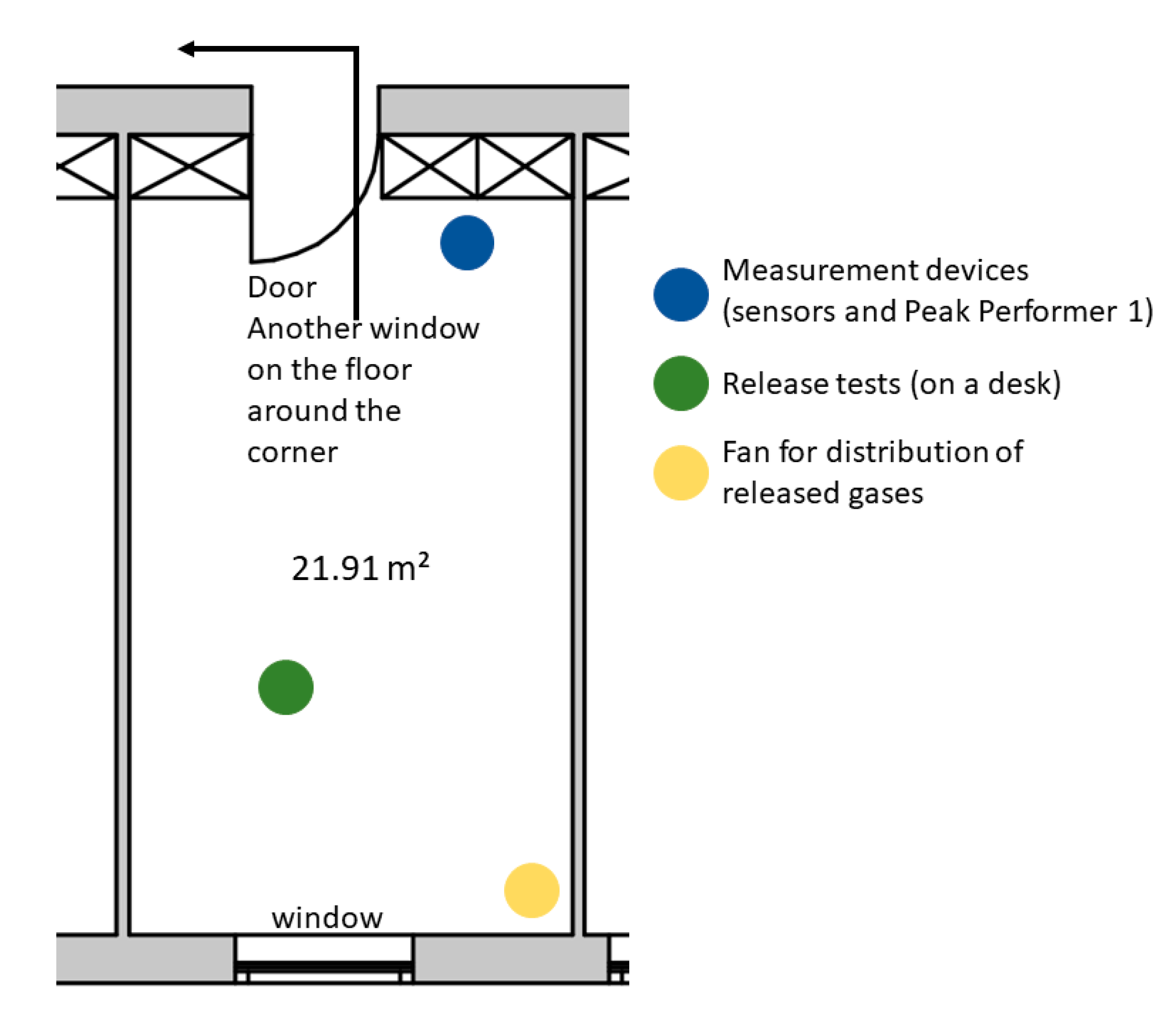
A plan of the field test room is shown in Figure 1. The area is 21.91 m2, the total volume of the room is 61.35 m3. The releases were performed close to the centre of the room and a fan from the corner was installed to produce some air flow and improve the (ideally uniform) distribution of released substances. From a CO2 release and the decay curve measured by NDIR CO2 sensors (SCD40, Sensirion AG, Stäfa, Switzerland) the air exchange rate with closed window and door is approximately 0.17 h−1.
3. Results
3.1. Lab Calibration
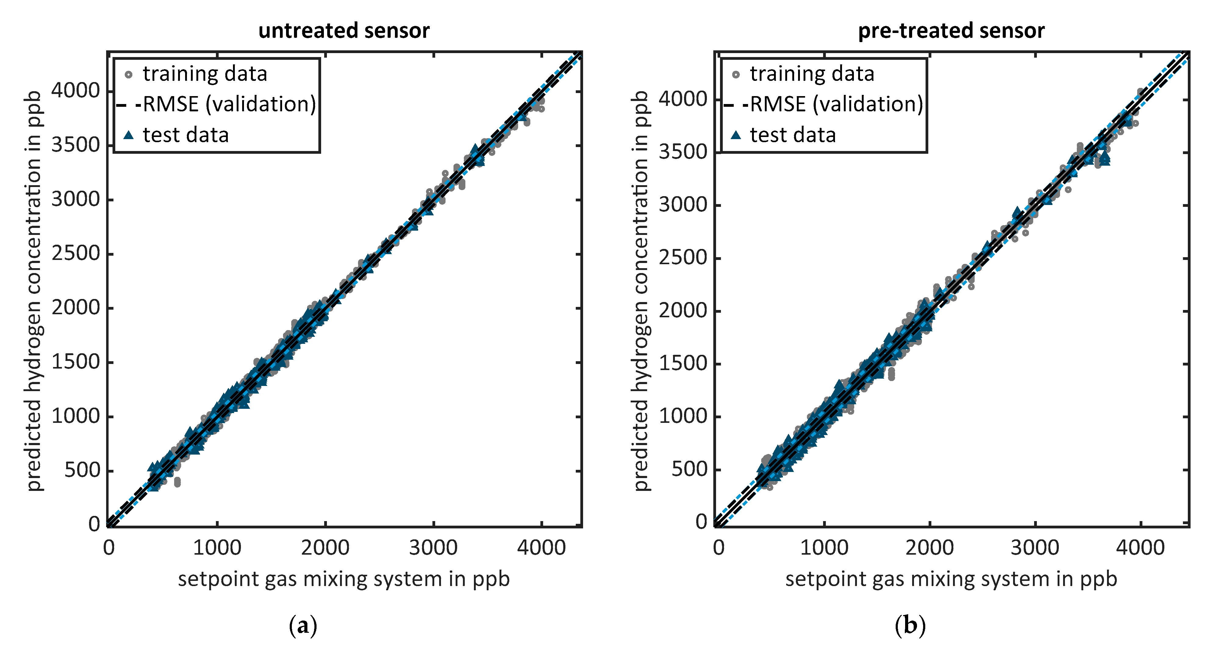
From the lab calibration the PLSR models shown in Figure 2 were obtained for both sensors. Each data point represents one cycle. The obtained values from the calibration are RMSEV = 44.8 ppb and RMSET = 40.5 ppb for the untreated sensor and RMSEV = 56.0 ppb and RMSET = 60.0 ppb for the pre-treated sensor. Since the pre-treatment enhances selectivity by reducing the sensitivity towards other gases more than towards H2, it is not surprising that quantification is somewhat worse for the pre-treated sensor. On the other hand, this sensor is chemically selective, whereas the untreated sensor might fail if gas compounds occur which were not part of the calibration dataset. Therefore, in the following we will always show both sensors, to check for synchronicity.
3.2. Validation in the Field
To check the functionality of the calibrated PLSR models directly in the field, we performed several H2 release tests. During the first two release tests no reference was available. Two consecutive releases were performed, the first one with a calculated concentration increase of 1 ppm inside the room and the second one with a calculated concentration increase of 2 ppm. These concentrations would be obtained if the gas released from the cylinder is evenly distributed inside the room and if there is no loss through ventilation, adsorption, or reaction; on average, somewhat lower values due to unavoidable losses are expected.
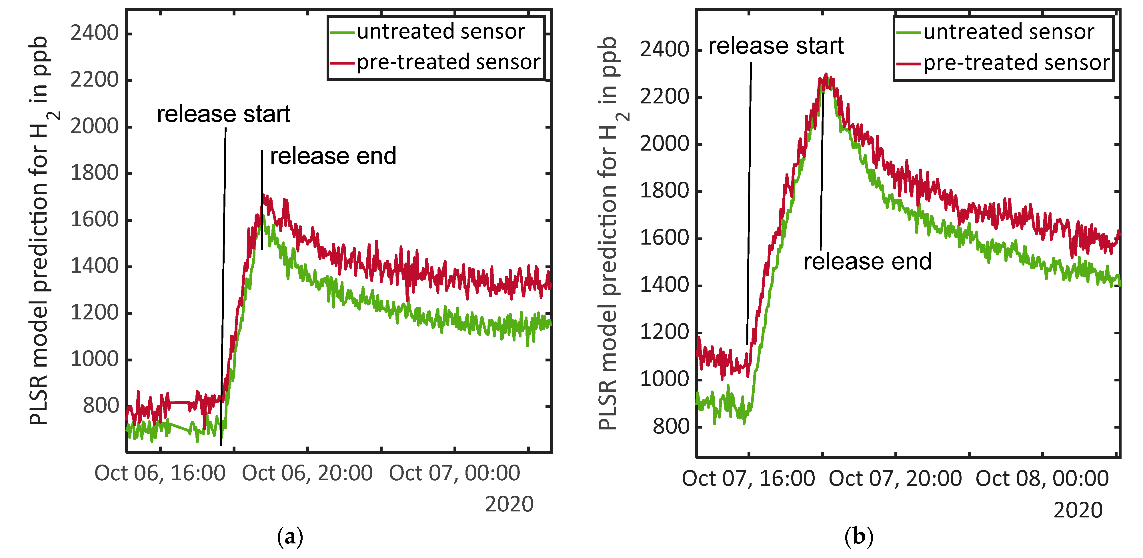
Figure 3a,b show the recorded concentration predictions based on the PLSR model during the first (1 ppm) and second release test (2 ppm), respectively; the start and end points of the releases are marked. The untreated sensor shows slightly (100–200 ppb) lower absolute values than the pre-treated sensor over the whole course. The H2 concentration increase during the first release is 900 ppb for the untreated sensor and 890 ppb for the pre-treated sensor. During the second H2 release the predicted increases are 1430 ppb and 1240 ppb for the untreated and pre-treated sensor, respectively.
During two periods a reference instrument (Peak Performer 1) was available. Figure 4a shows the first of these periods, where data from the reference instrument was recorded in parallel with both sensors over one weekend. While only minimal concentration changes were observed during that period, good correlation between all three signals is nevertheless evident. The untreated sensor shows an offset of approximately 200 ppb and only slightly higher noise than the analytical reference instrument. The pre-treated sensor shows an even higher offset of 500 ppb and, in accordance with the calibration results, a significantly higher noise level with almost double amplitude.
The second test period including the reference instrument is shown in Figure 4b. Again, we measured over one weekend, but this time some significant changes in H2 concentration were observed. Both sensor signals show a very good correlation to the reference device. On the final day a release test with a calculated concentration of 2 ppm H2 was performed. The room was thoroughly ventilated through open window and door before this release test. The reference instrument indicated a concentration increase during the release of 1465 ppb. The two sensors indicate an increase of 1650 ppb (untreated sensor) and 1365 ppb (pre-treated sensor). Despite the higher offset, the relative PLSR signal of the chemically selective MOS sensor correlates better with the analytical measurement (7% deviation vs. 13% deviation in the observed concentration increase).
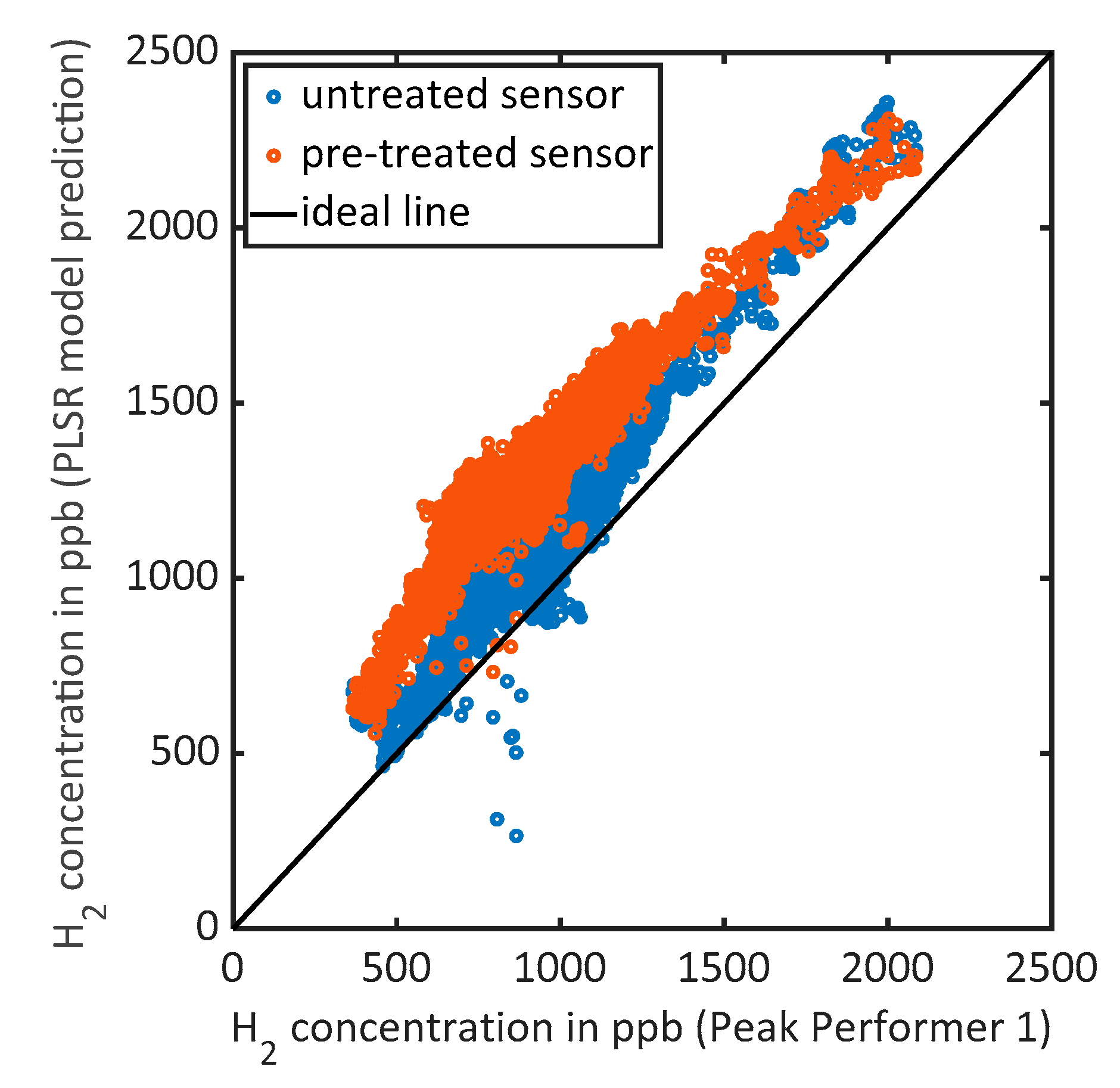
A correlation analysis over the whole period when the reference device was measuring in parallel was performed. Due to the different sampling rates (2 min for the sensors and 3.6 min for the Peak Performer 1) the data were resampled to obtain data points every minute using linear interpolation, Figure 5. From the 9560 data points per device (covering 160 h) Pearson correlation coefficients between the Peak Performer 1 and the PLSR model predictions from the untreated sensor and the pre-treated sensor were obtained of 0.97 and 0.95, respectively.
In field measurements it is impossible to gain uncertainty levels from noise calculation that are free of doubt because one cannot distinguish between changes in concentration and pure signal noise. However, we chose a 2 h window on 1 November with tolerably constant concentration level. A Lilliefors test was applied to the data points of all devices indicating they are normally distributed (5% significance level for rejection of the null hypothesis) so the assumption of constant concentration is reasonable [42]. The standard deviation of the Peak Performer 1 on that time scale is 15.9 ppb, which is close to the given accuracy of the instrument of 10 ppb. The untreated sensor shows a standard deviation of 29.8 ppb and the pre-treated sensor 36.1 ppb.
To judge the absolute accuracy of all three devices the ventilation event before the release test can be used. The atmosphere contains 500 ppb of H2 so lower levels are unrealistic—higher levels might be possible due to sources nearby (traffic or industry) [13,14]. The Peak Performer 1 shows a minimum concentration of 380 ppb during this ventilation, the untreated sensor 465 ppb and the pre-treated sensor 560 ppb. Thus, in this case the offset for the analytical reference device is at least −120 ppb and for the untreated sensor at least −35 ppb, the absolute accuracy of the pre-treated sensor cannot be determined.
3.3. Results during Field Tests
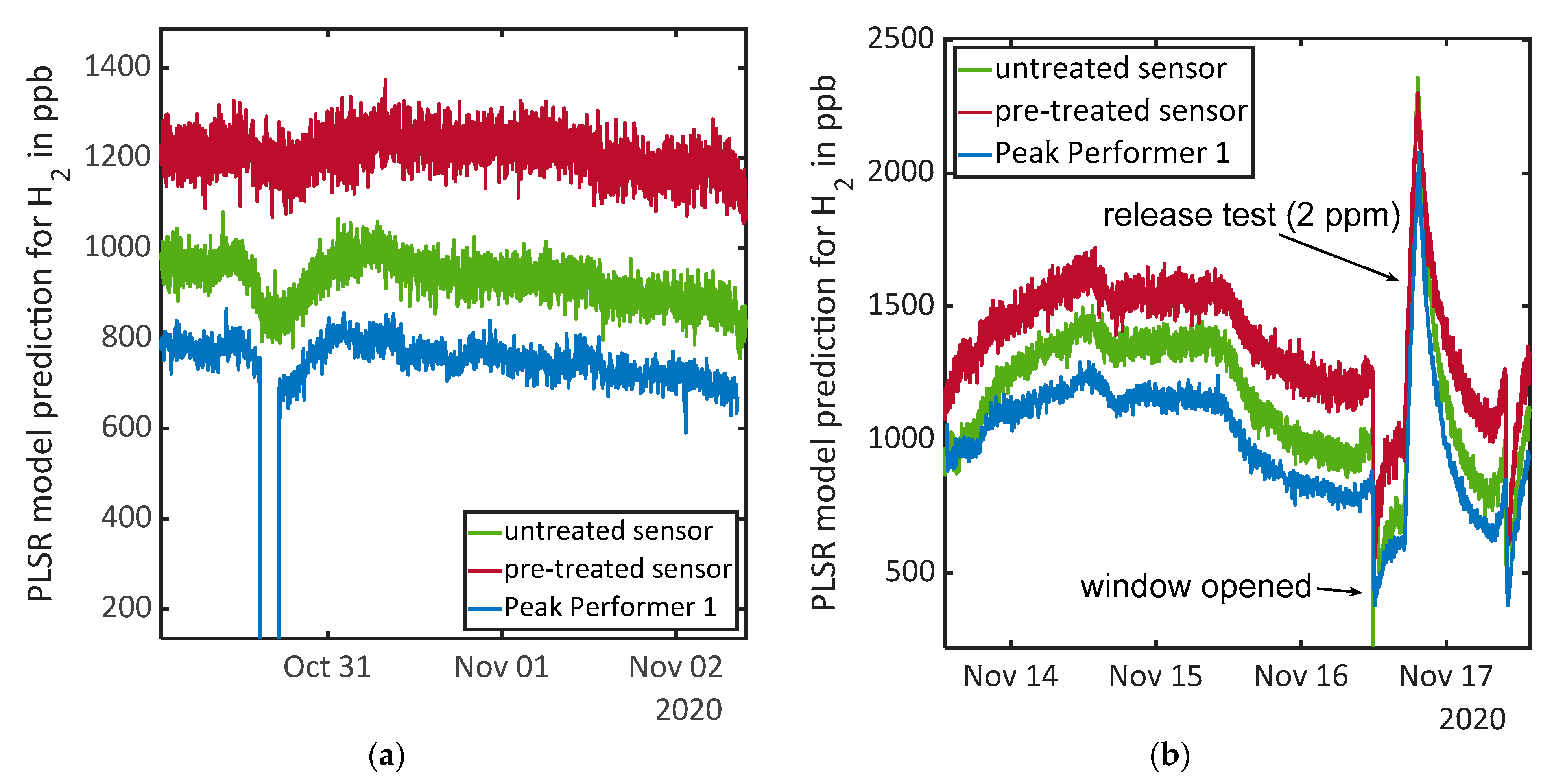
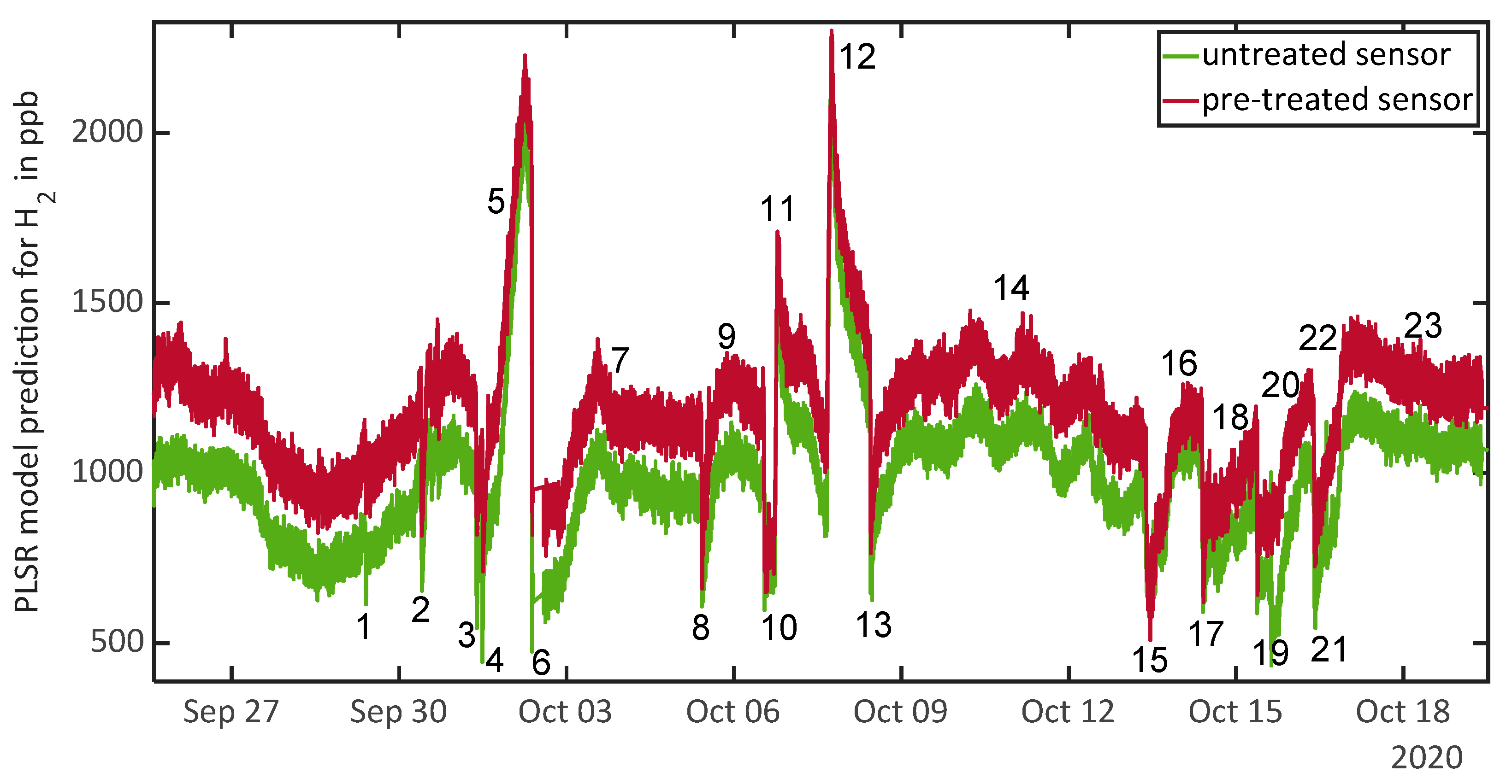
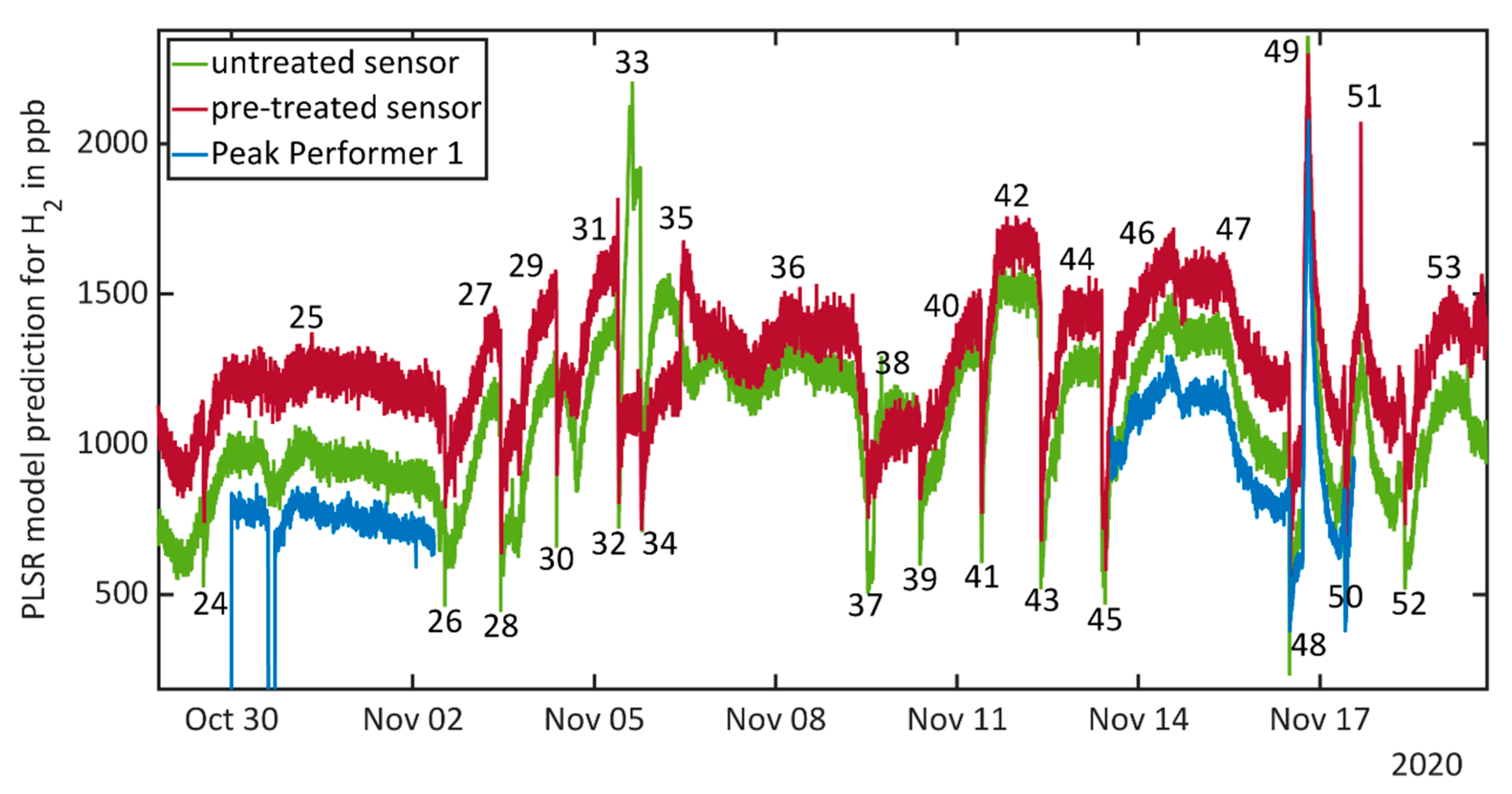
The first 25 days of the field test before the interim calibration is shown in Figure 6, the second part after that calibration spanning 22 days in Figure 7. Indicated H2 concentrations are between 450 ppb and 2300 ppb. During most of the time, the indicated concentration inside the room is around 1000 ppb, which is high compared to the atmospheric background level of 500 ppb. Numbers along the line mark events or periods, a detailed description of these in given in Appendix A, Table A1. All events labelled below the traces of the PLSR model predictions indicate ventilation events, i.e., the window and/or door of the room were opened, and the room thoroughly ventilated to achieve a clean baseline before and after the conducted release tests.
Events 11 and 12 indicate the H2 release tests shown in Figure 3a,b, #25 indicates the weekend with the data of the reference instrument recorded in parallel (cf. Figure 4a), and #47–49 the weekend and H2 release test with the second recording of the reference instrument in parallel (cf. Figure 4b).
Weekends are indicated by #7, 14, 23, 25, 36, and 47. During these days no one entered the room, and no release tests were conducted. Nevertheless, ascending as well as descending concentrations are observed, especially at #14, where oscillating values indicate a diurnal cycle. The maxima of these cycles are typically reached in the morning around 6–8 a.m., the corresponding minima in the evening around 6–8 p.m. During other weekends, this clear correlation with time is less obvious, but in general descending values are more likely in the afternoon.
During the field tests, release tests were also performed with different VOCs. The amount of evaporated liquid was always chosen to theoretically reach 600 ppb inside the room assuming ideal uniform distribution and no ventilation, corresponding to 0.1 to 0.16 mL. Here, an increase of the H2 concentration 2–6 h after the VOC release is observed. This increase often starts around 6 p.m., which is the same time at which the minimum in the diurnal cycle is observed. Looking at those days with release tests, during which a higher H2 concentration is observed than on the day before (#16, 20, 22, 27, 29, 31, 40, 42, and 46) a correlation to the substances acetone, isopropanol, toluene and xylene is found. Release of limonene (#35) results in an immediate increase of the PLSR output of the chemically selective pre-treated sensor, while the signal of the untreated sensor shows a less pronounced increase after 5–6 h.
Event 5 shows a strong increase in H2 concentration overnight after a day without any identified events or tests during that day. Event 33 shows a very strong increase of the H2 concentration prediction only from the untreated sensor while the signal obtained from the pre-treated sensor stays nearly constant. After ventilation (34) on the next day again a milder increase is observed with the same pattern. We were able to attribute these events to construction work inside the building using a binding agent, which was done on the same floor as the field test room on the first day and on the floor below on the second day.
Due to the Covid-19 pandemic no systematic investigation of the effect of human presence was possible. Only on some days (#9, 15, 29, and 45) individual persons sporadically entered the room and for every release test one person entered the room. However, in none of these cases could the human presence be observed from the H2 signal.
4. Discussion
Two questions arising from the results need to be discussed in more detail: (1) can MOS sensors function as reliable H2 detectors also in further research, and (2) what do we learn from the results concerning H2 in indoor environments?
Especially Figure 4—the PLSR predictions obtained from the MOS sensors recorded in parallel with an analytical reference instrument—strongly suggests, that the calibrated sensors can correctly measure relative fluctuations. For absolute measurements, an in-field one-point calibration might be sufficient to eliminate the observed but constant offset between the three devices. Similar to low-cost CO2 sensors, this could be realized with an automatic baseline correction, i.e., setting the lowest value over a longer period to the atmospheric background concentration. It is remarkable, that applying this approach during a ventilation event yields, that the analytical reference shows the highest offset from the baseline level of 500 ppb. Keeping in mind that the analytical device is three orders of magnitude more expensive than MOS sensors the performance of the sensors is very good with approximately doubled noise level compared to the analytical device and correlation coefficients of 0.95 and 0.97, respectively.
As the sensors are running parallel in almost all situations and given the very different methods of achieving the selective H2 signal, this also strongly implies the capability of MOS sensors to reliably measure H2 at least at ppm and sub-ppm concentrations. There are two events where significant deviations between both models occur: #33, where an emission during construction work was classified as H2 by the untreated sensor. In this situation, the chemically selective pre-treated sensor proves to be more reliable when untrained and unusual gases occur. During the release tests of limonene (#35), the opposite effect is observed: the model of the pre-treated sensor indicates an increase of H2, while the model of the untreated sensor remains at a constant value during the release and only indicates increasing values several hours after the release test. Since in contrast to all the other released gases we do not see any sensor reaction in the raw sensor data, we assume that the sealing membrane on the sensor prevents the large limonene molecules reaching the sensor surface. For the pre-treatment this membrane was removed, thus limonene can reach the hot sensor surface of the pre-treated sensor. We assume that limonene reacts on the hot surface releasing H2 (cf. [43]), resulting in a sensor response and an increase of the PLSR model prediction. Reapplying the sealing membrane would help to resolve this issue. Thus, in terms of selectivity the pre-treated sensor would be more reliable. In return a lower signal to noise ratio needs to be accepted. In contrast to a pre-treated sensor at constant temperature, which can be found in literature and suffers from low response times [30,44], the DSR mode overcomes this issue.
From the field tests we observe that releasing VOCs like toluene and acetone is followed by an increase in H2 concentration hours later. This might be due to decomposition processes such as photochemical oxidation [15]. However, this effect is also overlaid by the observed diurnal cycle with minimum H2 concentrations in the evening. This diurnal cycle is not fully correlated with the time of day, because we do not observe it every day. Probably also incident solar radiation, which is higher in the afternoon because the window is directed westwards, or temperature play a role. Therefore, high VOC levels probably also cause high H2 levels. During the field tests Tenax samples were drawn and analyzed by GC-MS, but no unusually high concentrations of any substance were found. Thus, the observed H2 base level inside the room, which was confirmed by the reference instrument to be significantly higher than atmospheric level, cannot be explained and is not fully understood. It seems that an unknown H2 source is inside the room as only lower concentrations were found in neighboring rooms and outside using the same sensors. Perhaps this high base level is caused by some unknown VOC source [16], e.g., from building materials or furniture, or by microorganisms, which can emit H2 from their metabolism (in fact, they are the cause for human H2 emissions).
Unfortunately, the observed changes of the H2 concentration overshadow all moments with human presence, which were short and only included one person. Thus, it was not possible to detect any effect of human presence against this background. In former experiments we found an increase of 2500 ppb over a span of 1 h in a room of similar size while 13 people were inside (same building, same floor). This correlates to an increase of approximately 200 ppb per person and hour. In a normal indoor air environment this can represent a valid indicator for human presence, but effects of VOC release, i.e., from cleaning agents would have to be considered. In any case, further experiments to determine H2 concentrations and fluctuations in different rooms under normal use (e.g., cooking, cleaning etc.) are required.
5. Conclusions
Two important conclusions can be drawn from the presented field test results: first, MOS sensors can reliably detect and quantify H2 in indoor environments; second, H2 is a dynamic parameter that needs more attention. More research is required on many open questions: Does H2 emitted by humans dominate in normal rooms so that it can be used as indicator for human presence? Does H2 represent a good indicator for other relevant and potentially harmful situations, e.g., high VOC values or microbial issues such as mold? Do many TVOC monitors based on MOS sensors, especially when driven at constant temperature, mainly measure H2?
Author Contributions
Conceptualization, C.S., T.B. and A.S.; methodology, C.S., T.B. and J.A.; software, T.B. and J.A.; validation, C.S., T.B. and J.A.; formal analysis, J.A.; investigation, J.A.; resources, A.S.; data curation, J.A.; writing—original draft preparation, C.S.; writing—review and editing, C.S., T.B. and A.S.; visualization, C.S. and J.A.; supervision, C.S., T.B. and A.S.; project administration, A.S. All authors have read and agreed to the published version of the manuscript.
Funding
This research received no external funding.
Institutional Review Board Statement
Not applicable.
Informed Consent Statement
Not applicable.
Data Availability Statement
The underlying data is available on Zenodo. DOI: 10.5281/zenodo.4593853. Title: Measuring Hydrogen in Indoor Air with a Selective Metal Oxide Semiconductor Sensor: Dataset. Authors: Johannes Amann, Tobias Baur, Caroline Schultealbert, https://zenodo.org/record/4593853. (accessed on 10 March 2021).
Acknowledgments
We thank Rainer Lammertz Pure Gas Products for providing the Peak Performer 1 reference instrument for this study.
Conflicts of Interest
The authors declare no conflict of interest.
Appendix A

Table A1.
List of all events (release tests, ventilation and other) during the field tests and the observed sensor behavior during that time.
Table A1.
List of all events (release tests, ventilation and other) during the field tests and the observed sensor behavior during that time.
| Number | Time | Type of event | Observation |
|---|---|---|---|
| 1 | 29 September, 09:35–09:48 | Door opened | Lower H2 concentration due to ventilation effect |
| 2 | 30 September, 09:24–09:58 | Window opened | Lower H2 concentration due to ventilation effect |
| 3 | 1 October, 09:10–09:30 | Window opened | Lower H2 concentration due to ventilation effect |
| 4 | 1 October, 11:47–12:05 | Door and window opened | Lower H2 concentration due to ventilation effect |
| 5 | 1 October, 18:30–2 October, 06:30 | No specifiable event | Strong increase of H2 concentration over night |
| 6 | 2 October, 09:00–09:30 | Door and window opened | Lower H2 concentration due to ventilation effect |
| 7 | 2 October, 14:00–5 October, 10:00 | Days without events and human presence | Maximum of H2 concentration at 3 October, 13:00 |
| 8 | 5 October, 10:10–10:30 | Door and window opened | Lower H2 concentration due to ventilation effect |
| 9 | 5 October and 6 October | Several short periods of human presence | No increasing H2 concentration for short presence of one person |
| 10 | 6 October, 13:08–16:51 | Door and window opened | Lower H2 concentration due to ventilation effect |
| 11 | 6 October, 17:42–18:44 | Release test: 1 ppm H2 | Compare Figure 3a |
| 12 | 7 October, 16:01–18:05 | Release test: 2 ppm H2 | Compare Figure 3b |
| 13 | 8 October, 10:46–11:00 | Door and window opened | Lower H2 concentration due to ventilation effect |
| 14 | 8 October to 13 October | Days without events and human presence | Oscillating H2 concentration with maximums typically around 06:00–08:00 and minimums typically around 18:00–20:00 |
| 15 | 13 October, 09:25–14:00 | Door and window opened, human presence | Lower H2 concentration due to ventilation effect |
| 16 | 13 October, 15:00 | Release test: toluene | Increase of H2 concentration 3 h after release (18:00) |
| 17 | 14 October, 09:30–10:05 | Door and window opened | Lower H2 concentration due to ventilation effect |
| 18 | 8 October to 13 October | Sporadic human presence, no specifiable events | Slow increase of H2 concentration over day and night |
| 19 | 15 October, 09:00–09:30 | Door and window opened | Lower H2 concentration due to ventilation effect |
| 20 | 15 October, 15:00 | Release test: acetone | Untreated sensor reacts to acetone release with a short peak and displays lower concentration afterwards. Three hours after release both sensors indicate increasing H2 concentration |
| 21 | 16 October, 09:40–10:10 | Door and window opened | Lower H2 concentration due to ventilation effect |
| 22 | 16 October, 14:50 and 18:00 | Release test: acetone and toluene | Untreated sensor reacts to release with a short peak and displays lower concentration afterwards. Five hours after first release both sensors indicate increasing H2 concentration |
| 23 | 17 October to 19 October | Days without events and human presence | Almost constant H2 concentration |
| 24 | 29 October, 12:55–13:10 | Door and window opened | Lower H2 concentration due to ventilation effect |
| 25 | 29 October to 2 November | Days without events and human presence | Almost constant H2 concentration |
| 26 | 2 November, 12:40–12:55 | Door and window opened | Lower H2 concentration due to ventilation effect |
| 27 | 2 November, 16:50 | Release test: toluene | Short reaction of untreated sensor upon release, constant increase of H2 concentration over day and night |
| 28 | 3 November, 10:55–11:10 | Door and window opened | Lower H2 concentration due to ventilation effect |
| 29 | 3 November, 15:30 | Release test: acetone followed by defect of the pump, human presence during fixing | Three hours after release test increase of H2 concentration (coincides with present person for pump fixing) |
| 30 | 4 November, 09:00–09:15 | Door and window opened | Lower H2 concentration due to ventilation effect |
| 31 | 4 November, 16:22 | Release test: acetone | Untreated sensor signal drops again upon release, increase of H2 concentration 2 h after release |
| 32 | 5 November, 09:26–09:41 | Door and window opened | Lower H2 concentration due to ventilation effect |
| 33 | 5 November, 15:10 | Release test: acetone and toluene. Unidentified event due to construction inside the building | Very strong increase in signal of the untreated sensor long before the release tests. Release then again causes a drop in the untreated sensor’s signal, and 2.5 h after release also the pre-treated sensor signal increases slightly. |
| 34 | 5 November, 18:30–18:50 | Door and window opened | Lower H2 concentration due to ventilation effect |
| 35 | 6 November, 10:03 | Release test: limonene | Pre-treated sensor detects limonene release immediately, untreated sensor shows increasing H2 concentration after 5–6 h, after 10 h signals go parallel again |
| 36 | 6 November to 9 November | Days without events and human presence | Almost constant H2 concentration, slight oscillation with maximum at 06:30 and minimums at 15:00 and 16:30 |
| 37 | 9 November, 12:21–13:01 | Door and window opened | Lower H2 concentration due to ventilation effect |
| 38 | 9 November, 18:00 | Release test: ethanol | One outlier towards higher concentration for untreated sensor upon release, almost constant H2 concentration |
| 39 | 10 November, 09:10–09:25 | Door and window opened | Lower H2 concentration due to ventilation effect |
| 40 | 10 November, 14:30 | Release test: isopopanol | Four hours after first release both sensors indicate increasing H2 concentration |
| 41 | 11 November, 09:28–09:48 | Door and window opened | Lower H2 concentration due to ventilation effect |
| 42 | 11 November, 15:49 | Release test: xylene | Increase of H2 concentration until release test, constant concentration afterwards |
| 43 | 12 November, 09:15–09:30 | Door and window opened | Lower H2 concentration due to ventilation effect |
| 44 | 12 November, 15:08 | Release test: toluene and xylene | Increase of the H2 concentration over the day (independent from release) and constant value after 19:00 |
| 45 | 13 November, 09:28–11:06 | Door and window opened | Lower H2 concentration due to ventilation effect |
| 46 | 13 November, 14:30 | Release test: acetone and ethanol | Small drop in sensor signal for untreated sensor, ascending H2 concentration over day and night |
| 47 | 13 November–16 November | Days without events and human presence | Decreasing H2 concentration between 13:30 and 17:00 on first day and after 11:30 over the whole night on second day |
| 48 | 16 November, 11:55–12:20 | Door and window opened | Lower H2 concentration due to ventilation effect |
| 49 | 16 November, 17:06–19:20 | Release test: 2 ppm H2 | Compare Figure 4b |
| 50 | 17 November, 09:54–10:24 | Door and window opened | Lower H2 concentration due to ventilation effect |
| 51 | 17 November, 18:24 | Release test: ethanol | Maximum in H2 concentration at 16:30, outlier in pre-treated signal due to pump switching, no signal change upon release, increasing H2 concentration after 06:30 |
| 52 | 18 November, 09:36–09:56 | Door and window opened | Lower H2 concentration due to ventilation effect |
| 53 | 19 November, 12:02–16:02 | Release test: carbon monoxide (tea candle) | Pre-treated sensor signal shows slight increase of H2 concentration during burning candle |
References
- Spaul, W.A. Building-related factors to consider in indoor air quality evaluations. J. Allergy Clin. Immunol. 1994, 94, 385–389. [Google Scholar] [CrossRef]
- Settimo, G.; Manigrasso, M.; Avino, P. Indoor Air Quality: A Focus on the European Legislation and State-of-the-Art Research in Italy. Atmosphere 2020, 11, 370. [Google Scholar] [CrossRef] [Green Version]
- World Health Organization. WHO Air Quality Guidelines for Particulate Matter, Ozone, Nitrogen Dioxide and Sulfur Dioxide: Global Update 2005: Summary of Risk Assessment; World Health Organization: Geneva, Switzerland, 2006. [Google Scholar]
- Krzyzanowski, M.; Cohen, A. Update of WHO air quality guidelines. Air Qual. Atmos. Health 2008, 1, 7–13. [Google Scholar] [CrossRef] [Green Version]
- Pettenkofer, M. Besprechung Allgemeiner auf die Ventilation bezüglicher Fragen; J.G. Cottaísche Buchhandlung: München, Germany, 1858. [Google Scholar]
- Szczurek, A.; Maciejewska, M.; Pietrucha, T. CO2 and Volatile Organic Compounds as indicators of IAQ. In Proceedings of the 36th AIVC Conference—Effective Ventilation in High Performance Buildings, Madrid, Spain, 23–24 September 2015; pp. 118–127. [Google Scholar]
- Rovelli, S.; Cattaneo, A.; Fazio, A.; Spinazzè, A.; Borghi, F.; Campagnolo, D.; Dossi, C.; Cavallo, D. VOCs Measurements in Residential Buildings: Quantification via Thermal Desorption and Assessment of Indoor Concentrations in a Case-Study. Atmosphere 2019, 10, 57. [Google Scholar] [CrossRef] [Green Version]
- Scully, R.R.; Basner, M.; Nasrini, J.; Lam, C.; Hermosillo, E.; Gur, R.C.; Moore, T.; Alexander, D.J.; Satish, U.; Ryder, V.E. Effects of acute exposures to carbon dioxide on decision making and cognition in astronaut-like subjects. NPJ Microgravity 2019, 5, 17. [Google Scholar] [CrossRef]
- Liu, Y.; Misztal, P.K.; Xiong, J.; Tian, Y.; Arata, C.; Weber, R.J.; Nazaroff, W.W.; Goldstein, A.H. Characterizing sources and emissions of volatile organic compounds in a northern California residence using space- and time-resolved measurements. Indoor Air 2019, 29, 630–644. [Google Scholar] [CrossRef] [Green Version]
- Leidinger, M.; Sauerwald, T.; Reimringer, W.; Ventura, G.; Schütze, A. Selective detection of hazardous VOCs for indoor air quality applications using a virtual gas sensor array. J. Sens. Sens. Syst. 2014, 3, 253–263. [Google Scholar] [CrossRef] [Green Version]
- Schütze, A.; Baur, T.; Leidinger, M.; Reimringer, W.; Jung, R.; Conrad, T.; Sauerwald, T. Highly Sensitive and Selective VOC Sensor Systems Based on Semiconductor Gas Sensors: How to? Environments 2017, 4, 20. [Google Scholar] [CrossRef] [Green Version]
- Lee, A.P.; Reedy, B.J. Temperature modulation in semiconductor gas sensing. Sens. Actuators B Chem. 1999, 60, 35–42. [Google Scholar] [CrossRef]
- Schleyer, R.; Bieber, E.; Wallasch, M. Das Luftmessnetz des Umweltbundesamtes; Umweltbundesamt: Dessau-Roßlau, Germany, 2013. [Google Scholar]
- Barnes, D.H.; Wofsy, S.C.; Fehlau, B.P.; Gottlieb, E.W.; Elkins, J.W.; Dutton, G.S.; Novelli, P.C. Hydrogen in the atmosphere: Observations above a forest canopy in a polluted environment. J. Geophys. Res. Space Phys. 2003, 108, 4197. [Google Scholar] [CrossRef] [Green Version]
- Ehhalt, D.H.; Rohrer, F. The tropospheric cycle of H 2: A critical review. Tellus B Chem. Phys. Meteorol. 2009, 61, 500–535. [Google Scholar] [CrossRef]
- Grant, A.; Archibald, A.T.; Cooke, M.C.; Nickless, G.; Shallcross, D.E. Modelling the oxidation of 15 VOCs to track yields of hydrogen. Atmos. Sci. Lett. 2010, 11, 265–269. [Google Scholar] [CrossRef]
- Forster, G.L.; Sturges, W.T.; Fleming, Z.L.; Bandy, B.J.; Emeis, S. A year of H 2 measurements at Weybourne Atmospheric Observatory, UK. Tellus B Chem. Phys. Meteorol. 2012, 64, 17771. [Google Scholar] [CrossRef] [Green Version]
- Marthinsen, D.; Fleming, S.E. Excretion of Breath and Flatus Gases by Humans Consuming High-Fiber Diets. J. Nutr. 1982, 112, 1133–1143. [Google Scholar] [CrossRef]
- Tomlin, J.; Lowis, C.; Read, N.W. Investigation of normal flatus production in healthy volunteers. Gut 1991, 32, 665–669. [Google Scholar] [CrossRef] [Green Version]
- Tadesse, K.; Smith, D.; Eastwood, M.A. Breath Hydrogen and Methane Excretion Patterns in Normal man and in Clinical Practices. J. Expimental Physiol. 1980, 65, 85–97. [Google Scholar] [CrossRef] [Green Version]
- Levitt, M.D. Production and excretion of hydrogen gas in man. N. Engl. J. Med. 1969, 281, 122–127. [Google Scholar] [CrossRef]
- Sone, Y.; Tanida, S.; Matsubara, K.; Kojima, Y.; Kato, N.; Takasu, N.; Tokura, H. Everyday Breath Hydrogen Excretion Profile in Japanese Young Female Students. J. Physiol. Anthr. Appl. Hum. Sci. 2000, 19, 229–237. [Google Scholar] [CrossRef]
- Appel, J.; Schulz, R. Hydrogen metabolism in organisms with oxygenic photosynthesis: Hydrogenases as important regulatory devices for a proper redox poising? J. Photochem. Photobiol. B Biol. 1998, 47, 1–11. [Google Scholar] [CrossRef]
- Nandi, R.; Sengupta, S. Microbial Production of Hydrogen: An Overview. Crit. Rev. Microbiol. 1998, 24, 61–84. [Google Scholar] [CrossRef]
- Rüffer, D.; Hoehne, F.; Bühler, J. New digital metal-oxide (MOx) sensor platform. Sensors 2018, 18, 1052. [Google Scholar] [CrossRef] [Green Version]
- Schultealbert, C.; Baur, T.; Schütze, A.; Sauerwald, T. Investigating the role of hydrogen in the calibration of MOS gas sensors for indoor air quality monitoring. In Proceedings of the Indoor Air Conference, Philadelphia, PA, USA, 22–27 July 2018. [Google Scholar]
- Meng, X.; Zhang, Q.; Zhang, S.; He, Z. The Enhanced H2 Selectivity of SnO2 Gas Sensors with the Deposited SiO2 Filters on Surface of the Sensors. Sensors 2019, 19, 2478. [Google Scholar] [CrossRef] [PubMed] [Green Version]
- Schultealbert, C.; Uzun, I.; Baur, T.; Sauerwald, T.; Schütze, A. Siloxane treatment of metal oxide semiconductor gas sensors in temperature-cycled operation—Sensitivity and selectivity. J. Sens. Sens. Syst. 2020, 9, 283–292. [Google Scholar] [CrossRef]
- Hyodo, T.; Baba, Y.; Wada, K.; Shimizu, Y.; Egashira, M. Hydrogen sensing properties of SnO2 varistors loaded with SiO2 by surface chemical modification with diethoxydimethylsilane. Sens. Actuators B Chem. 2000, 64, 175–181. [Google Scholar] [CrossRef]
- Tournier, G.; Pijolat, C. Selective filter for SnO-based gas sensor: Application to hydrogen trace detection. Sens. Actuators B Chem. 2005, 106, 553–562. [Google Scholar] [CrossRef] [Green Version]
- Katsuki, A.; Fukui, K. H2 selective gas sensor based on SnO2. Sens. Actuators B Chem. 1998, 52, 30–37. [Google Scholar] [CrossRef]
- Schultealbert, C.; Baur, T.; Schütze, A.; Böttcher, S.; Sauerwald, T. A novel approach towards calibrated measurement of trace gases using metal oxide semiconductor sensors. Sens. Actuators B Chem. 2017, 239, 390–396. [Google Scholar] [CrossRef]
- Schultealbert, C.; Baur, T.; Schütze, A.; Sauerwald, T. Facile Quantification and Identification Techniques for Reducing Gases over a Wide Concentration Range Using a MOS Sensor in Temperature-Cycled Operation. Sensors 2018, 18, 744. [Google Scholar] [CrossRef] [Green Version]
- Baur, T.; Schultealbert, C.; Schütze, A.; Sauerwald, T. Novel method for the detection of short trace gas pulses with metal oxide semiconductor gas sensors. J. Sens. Sens. Syst. 2018, 7, 411–419. [Google Scholar] [CrossRef]
- Bastuck, M.; Baur, T.; Schütze, A. DAV3E—A MATLAB toolbox for multivariate sensor data evaluation. J. Sens. Sens. Syst. 2018, 7, 489–506. [Google Scholar] [CrossRef] [Green Version]
- Amann, J. Möglichkeiten und Grenzen des Einsatzes von Halbleitergassensoren im temperaturzyklischen Betrieb für die Messung der Innenraumluftqualität—Kalibrierung, Feldtest, Validierung. Master’s Thesis, Universität des Saarlandes, Saarbrücken, Germany, 2021. [Google Scholar]
- Bastuck, M. Improving the Performance of Gas Sensor Systems with Advanced Data Evaluation, Operation, and Calibration Methods; Shaker Verlag GmbH: Düren, Germany, 2019; ISBN 978-3-8440-7075-0. [Google Scholar]
- Leidinger, M.; Schultealbert, C.; Neu, J.; Schütze, A.; Sauerwald, T. Characterization and calibration of gas sensor systems at ppb level—a versatile test gas generation system. Meas. Sci. Technol. 2018, 29, 015901. [Google Scholar] [CrossRef] [Green Version]
- Helwig, N.; Schüler, M.; Bur, C.; Schütze, A.; Sauerwald, T. Gas mixing apparatus for automated gas sensor characterization. Meas. Sci. Technol. 2014, 25, 055903. [Google Scholar] [CrossRef]
- Baur, T.; Bastuck, M.; Schultealbert, C.; Sauerwald, T.; Schütze, A. Random gas mixtures for efficient gas sensor calibration. J. Sens. Sens. Syst. 2020, 9, 411–424. [Google Scholar] [CrossRef]
- Loh, W.-L. On Latin Hypercube Sampling. Ann. Stat. 1996, 24, 2058–2080. [Google Scholar] [CrossRef]
- Lilliefors, H.W. On the Kolmogorov-Smirnov Test for Normality with Mean and Variance Unknown. J. Am. Stat. Assoc. 1967, 62, 399–402. [Google Scholar] [CrossRef]
- Martin-Luengo, M.A.; Yates, M.; Rojo, E.S.; Huerta Arribas, D.; Aguilar, D.; Ruiz Hitzky, E. Sustainable p-cymene and hydrogen from limonene. Appl. Catal. A Gen. 2010, 387, 141–146. [Google Scholar] [CrossRef]
- Fleischer, M.; Kornely, S.; Weh, T.; Frank, J.; Meixner, H. Selective gas detection with high-temperature operated metal oxides using catalytic filters. Sens. Actuators B Chem. 2000, 69, 205–210. [Google Scholar] [CrossRef]
Figure 1.
Field test room and positions of the measurement devices, release tests, and a fan for improved distribution of the evaporated substances inside the room.
Figure 1.
Field test room and positions of the measurement devices, release tests, and a fan for improved distribution of the evaporated substances inside the room.

Figure 2.
Partial least squares regression (PLSR) models for the prediction of H2 concentration based on the calibration inside the lab: (a) untreated sensor: root mean squared error for validation (RMSEV) = 44.8 ppb and RMSET = 40.5 ppb; (b) sensor pre-treated with siloxane: RMSEV = 56.0 ppb and RMSET = 60.0 ppb. Grey circles are part of the training, blue triangles part of the independent test data (20% of the data); both PLSR models show no indication of overfitting.

Figure 3.
PLSR model predictions for H2 for both sensors (untreated and pre-treated) during two release tests of H2 supplied from a pressure cylinder with constant rate provided by a mass flow controller: (a) first release with calculated increase of 1 ppm; (b) second release with calculated increase of 2 ppm.

Figure 4.
PLSR model predictions for H2 for both sensors (untreated and pre-treated) compared to an analytical reference instrument (Peak Performer 1): (a) a weekend without additional events, the reference instrument was not connected to the pump for a short period of time and indicates 0 ppb during that period; (b) during a weekend followed by a release test with a calculated concentration increase of 2 ppm H2.

Figure 5.
Concentrations obtained from the PLSR model predictions of both sensors vs. concentration indicated by the Peak Performer 1.
Figure 5.
Concentrations obtained from the PLSR model predictions of both sensors vs. concentration indicated by the Peak Performer 1.

Figure 6.
PLSR model predictions for H2 from both sensors (untreated and pre-treated) over several days. Descriptions of the labelled events and periods can be found in Appendix A, Table A1.
Figure 6.
PLSR model predictions for H2 from both sensors (untreated and pre-treated) over several days. Descriptions of the labelled events and periods can be found in Appendix A, Table A1.

Figure 7.
PLSR model predictions for H2 from both sensors (untreated and pre-treated) over several days. Descriptions of the labelled events and periods can be found in Appendix A, Table A1.
Figure 7.
PLSR model predictions for H2 from both sensors (untreated and pre-treated) over several days. Descriptions of the labelled events and periods can be found in Appendix A, Table A1.

Publisher’s Note: MDPI stays neutral with regard to jurisdictional claims in published maps and institutional affiliations. |
© 2021 by the authors. Licensee MDPI, Basel, Switzerland. This article is an open access article distributed under the terms and conditions of the Creative Commons Attribution (CC BY) license (http://creativecommons.org/licenses/by/4.0/).
Share and Cite
MDPI and ACS Style
Schultealbert, C.; Amann, J.; Baur, T.; Schütze, A. Measuring Hydrogen in Indoor Air with a Selective Metal Oxide Semiconductor Sensor. Atmosphere 2021, 12, 366. https://0-doi-org.brum.beds.ac.uk/10.3390/atmos12030366
AMA Style
Schultealbert C, Amann J, Baur T, Schütze A. Measuring Hydrogen in Indoor Air with a Selective Metal Oxide Semiconductor Sensor. Atmosphere. 2021; 12(3):366. https://0-doi-org.brum.beds.ac.uk/10.3390/atmos12030366
Chicago/Turabian StyleSchultealbert, Caroline, Johannes Amann, Tobias Baur, and Andreas Schütze. 2021. "Measuring Hydrogen in Indoor Air with a Selective Metal Oxide Semiconductor Sensor" Atmosphere 12, no. 3: 366. https://0-doi-org.brum.beds.ac.uk/10.3390/atmos12030366
Note that from the first issue of 2016, this journal uses article numbers instead of page numbers. See further details here.