1. Introduction
Since the 1960s, terrestrial mosses have been used for monitoring studies of atmospheric metallic deposition at different scales [
1,
2]. Their morphological and physiological properties make them excellent sensors of atmospheric contaminants in particulate or soluble form. The lack of a root and vascular system makes them dependent on the atmospheric deposition for their nutrients. Mosses efficiently uptake and retain their essential elements, but simultaneously capture many other elements such as metals [
3,
4]. Moss biomonitoring is a comparative method which makes it possible to rank the sites relative to one another according to the concentration value measured in the samples [
5]. It is traditionally accepted that these values are quantitative estimates of atmospheric deposition. At the European scale, some studies, using Spearman rank correlations and multivariate decision trees, showed that atmospheric deposition modeled by the European Monitoring and Evaluation Programme (EMEP) is the main factor determining the accumulation of cadmium (Cd) and lead (Pb) in pleurocarpous mosses (
Pleurozium schreberi,
Hylocomium splendens,
Hypnum cupressiforme, and
Pseudoscleropodium purum) in rural areas and far from emission sources [
6,
7,
8]. Similarly, in rural areas at the scale of certain countries (Germany, Switzerland, Bulgaria, and Spain, for example), regression or correlation approaches, linking the concentrations measured in pleurocarpous mosses to the deposition data modeled by EMEP for Cd and Pb, also demonstrated a moderate or high significant correlation between these matrices and that the value of this link depends on the country [
9,
10,
11,
12]. However, it is necessary to take these results with caution because the relationship between metal concentrations accumulated by mosses and atmospheric deposition is complex and dependent on several factors such as age of mosses or part of analyzed mosses [
5,
13].
Nevertheless, these previous studies on the main factors determining the accumulation of Cd in pleurocarpous mosses have been carried out in rural and forest areas and far from emissions sources. Moss data can be used in human health studies because they make it possible to overcome the limitations of data sets concerning atmospheric metals. According to the European Directive 2004/107/EC and 2008/50/EC, only five metals are statutorily followed by physicochemical methods, and the modeled deposit maps over a large territory therefore only concern a few elements [
14,
15]. Human cohort studies are mainly carried out in urban and peri-urban areas [
16], and it is therefore necessary to adapt the protocols used in rural areas to urban areas. Few studies using mosses as a passive bioaccumulator (mosses growing on a given site are directly collected and analyzed [
17]) have been carried out in urban areas, but most of them used moss species of the
Grimmia Hedw. genus [
18,
19,
20]. These species are abundant in urban and peri-urban environments on stone or cement-based supports and can live in contaminated environments.
In this study, we have more particularly studied the accumulation of Cd by species of the
Grimmia genus in the urban area associated with two French metropolitan areas: Paris and Lyon. Indeed, Cd is an element of essentially anthropogenic origin emitted mainly by road traffic, industry, and the residential sector [
21] and recognized as carcinogenic element [
22]. Moreover, in rural areas, a recent study demonstrated a positive association between Cd and mortality [
14]. Mosses are collected in cemeteries which represent relatively homogeneous areas and in which, depending on the management mode, mosses can remain for long periods [
19]. Moreover, cemeteries share common traits in all cities although their characteristics can vary at the local level (proximity to a road, an industry, a crop, use of phytosanitary products, etc.). Natali et al. [
19] demonstrated that in Île-de-France (Paris metropolitan area),
Grimmia pulvinata (Hedw.) Sm. collected from cemeteries was an effective bioaccumulator for studying the spatial variability of metal deposits.
For the first time, we will study more precisely the relationship between the Cd accumulated by mosses of the genus
Grimmia in urban area and atmospheric Cd concentrations modeled by CHIMERE [
23]. CHIMERE is a chemistry transport model designed for regional atmospheric composition [
24]. Pollutant emissions, advection and mixing, chemistry, and deposition are the key processes affecting the chemical concentrations outputs provided by the model. Many research applications (transport, mixing, turbulence, chemistry, etc.) as well as operational forecasts (air quality networks, etc.) are based on CHIMERE, working either online or offline. In this application, CHIMERE temporal and spatial grids were used to evaluate air concentration of Cd in the study areas of Paris and Lyon. Then, we will design and test statistical models explaining the relationship between atmospheric modeled Cd and accumulated Cd in the two biggest metropolitan areas of France: Paris and Lyon. These models will consider stationary variables such as, for example, the altitude of the site, the type of support on which the mosses were taken, the distance to the center of the zone, as well as the measurement of Cd uncertainties. Finally, we will study the best model defined for Paris metropolitan area on the metropolitan area of Lyon (and reversing the cities) to verify the potential regionalization of the responses of mosses to Cd metallic contaminant.
2. Materials and Methods
2.1. Cd Measurements in Mosses in Cemeteries of Paris and Lyon Metropolitan Areas
2.1.1. Studied Sites
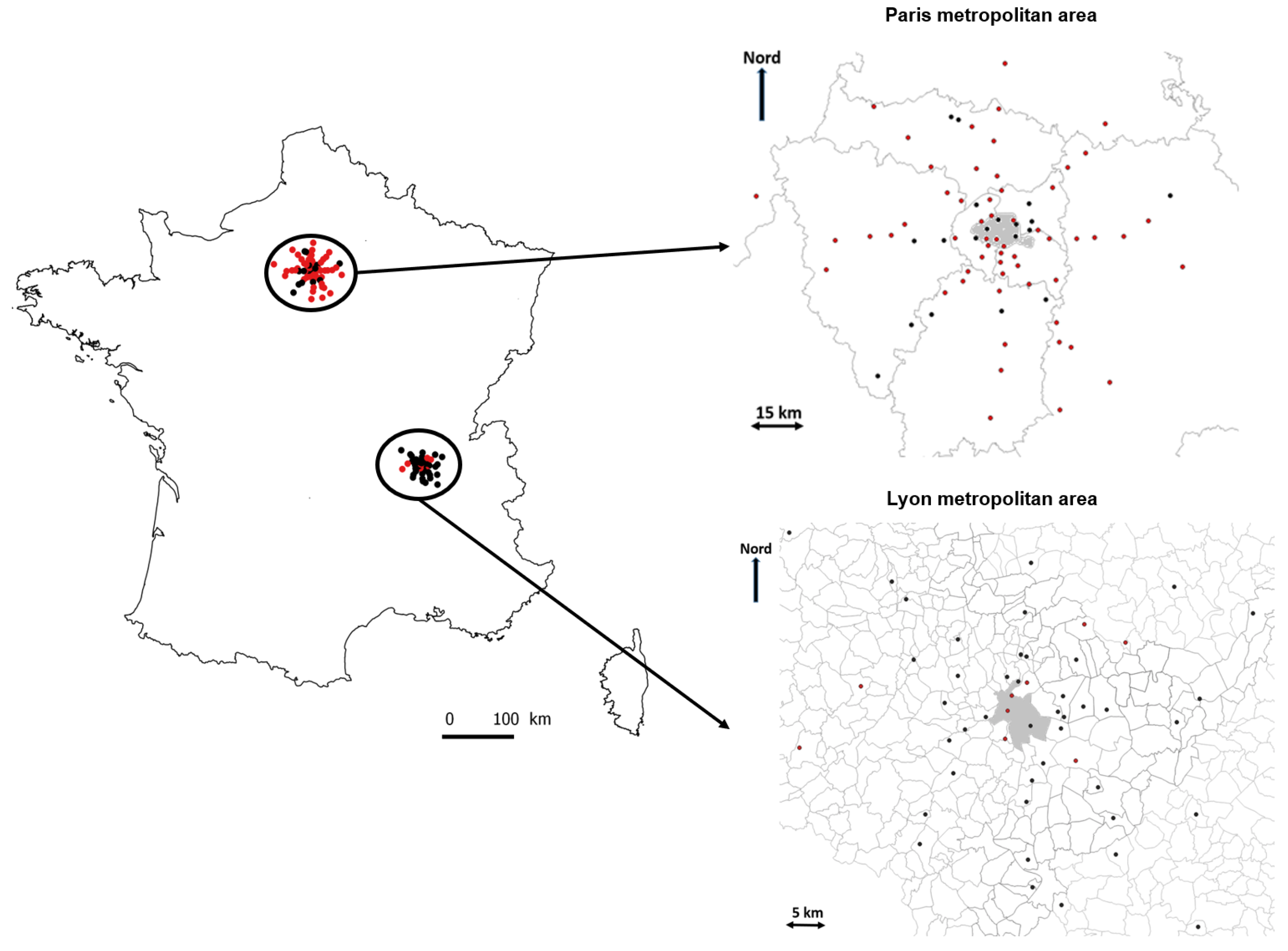
The studied areas (
Figure 1) are defined according to the population density based on INSEE criteria. Briefly, 4 categories of spatial units are defined: residential zones (between 2000 and 5000 inhabitants), industrial or commercial activity zones (sparsely populated or with 1000 employees), sparsely populated recreation zones, and municipalities with have not been divided according to the previous criteria (
https://www.insee.fr/fr/information/2383389 (accessed on 13 April 2021)). For these municipalities, their population density made it possible to divide them into 4 classes of high population density with very low population density. Each of the studied areas correspond to a circular surface whose center coincides with the barycentre of the continuous area of high and moderate population density (urban and peri-urban area). For Paris metropolitan area, the studied area is delimited by a circle with a radius of 49 km, the origin of which is located in Paris (Montparnasse Cemetery). This area covers all the departments of the so-called “Île de France” area. For Lyon metropolitan area, the studied area is delimited by a circle with a radius of 30 km, centered in Lyon city.
2.1.2. Moss Sampling and Analysis
All moss samples in Paris and Lyon metropolitan area were, respectively, collected during 3 weeks in May 2018 and 15 consecutive days in June 2018. The moss species collected is Grimmia pulvinata. All collected samples are exclusively bryophytic colonies developed on substrates whose composition is cement, mortar, or concrete. Two types of support were sampled: tombs and the flat top of the perimeter walls. For a given site, all the moss colonies are taken from the same support (graves or walls). The walls were chosen as the preferential support for harvesting mosses. To avoid risks of elemental transfers by water runoff, attention was paid that no overhanging tree canopy or surface was present above sampled moss cushions. Mosses directly under the influence of metallic objects (flowerpots, religious objects, etc.) were rejected. In the Paris metropolitan area, mosses were collected from graves in 58 cemeteries and from walls in 19 cemeteries. In the Lyon metropolitan area, mosses were collected from graves in 9 cemeteries and from walls in 42 cemeteries.
Each moss sample is made up of a minimum of 50 distinct colonies. The colonies are stored in a double-sealed zip bag and are stored in a cooler while awaiting return to the laboratory and placing them in a cold room at 4
C. In the laboratory, they are dried at room temperature. Then, non-moss organic matter debris and gravels are removed. Whole shoots of moss samples are then ground with an automatic non-polluting titanium grinder (Pulverisette 14, Fritsch, Germany). To avoid any accidental contamination of our samples, they are taken and then handled with nitrile gloves and ceramic knives and a scalpel. A total of 250 mg of homogeneous powder is mineralized with a mixture of HF/HNO
/H
O
. Cadmium (Cd) in mosses has been analyzed by inductively coupled plasma mass spectrometry (ICP-MS) by the USRAVE (INRAE- Centre de Bordeaux) (Limit of quantification is 0.02
g/g). The device used by the USRAVE is an Agilent 7700x spectrometer. The ICP-MS is calibrated by external calibration, using multi-element solutions produced every 6 months. The internal calibration procedure involves the addition of the standard to obtain the same concentration in each sample, thus allowing the monitoring of the good performance of the device and the correction of drift over time. In this study, certified reference materials for trace elements (CRMs), namely, NIST 1547 (peach leaves), NIST 1573a (Tomato leaves), as well as European moss survey program reference materials—Moss M2 and Moss M3—were processed with each batch of samples. The Moss M2 and Moss M3 standards are powders of
Pleurozium schreberi from two Finnish sites [
25].
2.2. Atmospheric Cd Forecasts from Chimere Chemistry Transport Model
CHIMERE is an open source multi-scale mesoscale physico-chemistry model, jointly developed as a National Tool of the French Institut des Sciences de l’Univers, by IPSL/LMD (Palaiseau), INERIS (Verneuil en Halatte) and IPSL/LISA (Creteil) in France. The source code and the associated documentation are available on the website
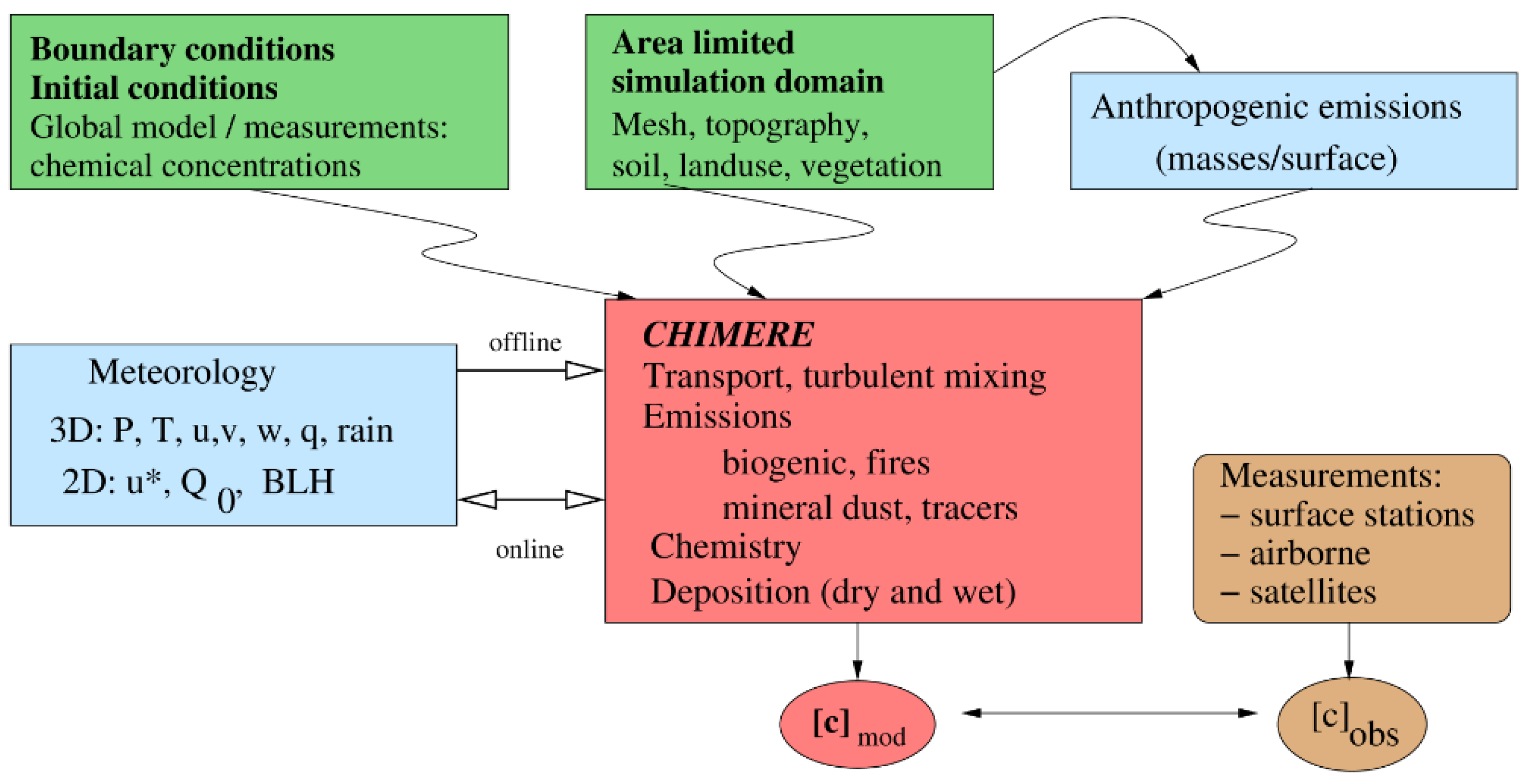
http://www.lmd.polytechnique.fr/chimere (accessed on 13 April 2021). It simulates the troposphere (the first atmospheric layer of 10 km of altitude) with various horizontal resolutions over study areas ranging from city to continent. The CHIMERE model [
24,
26] solves integro-differential partial equations, coupled with meteorological forcing covariates and various sources of anthropogenic or natural emissions (
Figure 2). The numerical code is parallelized and can deal with long-term simulations of the future behavior of many chemical elements, gases, and aerosols [
27], as well as short-term operational forecasting of atmospheric pollution [
28].
As main outputs, CHIMERE can deliver hourly pollutant concentrations (gases and aerosols) in 3D on any simulation domain. The various pollutants commonly monitored for atmospheric pollution can be simulated: O
, NO, NO
, SO
, PM
, PM
, and much more in dedicated CHIMERE versions, like some heavy metals (Pb, Cd, As, Ni, Cu, Zn, Cr, and Se) [
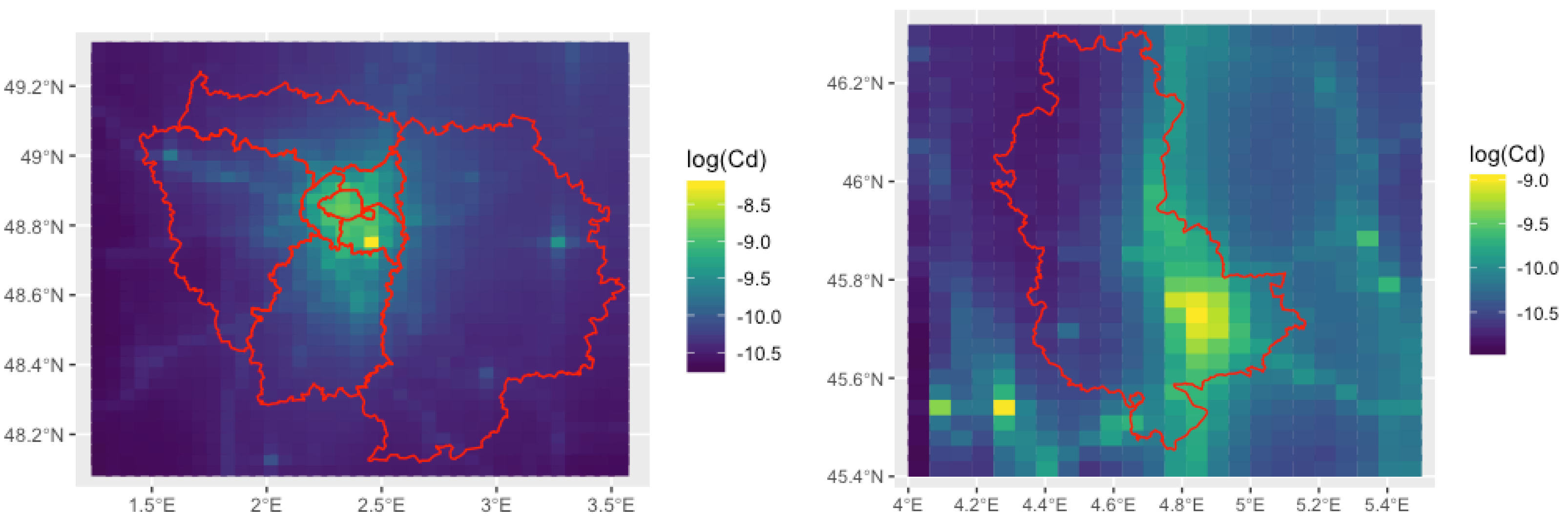
26]. The retrospective work hereafter focuses on Cd: CHIMERE was therefore launched to provide monthly series of Cd concentrations in the air during year 2015 under the form of twelve 240 × 324 pixel grids covering the mainland of France in Europe.
In France, there are 4 main sources of Cd emissions: the manufacturing industry, energy transformation (incineration plants), road transport, and residential sector [
21]. The CHIMERE model is based on the real emissions of Cd by each sector and industry, so each Cd data synthesizes the influence of each Cd source at a given pixel.
2.3. Defining the Area of Influence of the Atmospheric Cd on Mosses
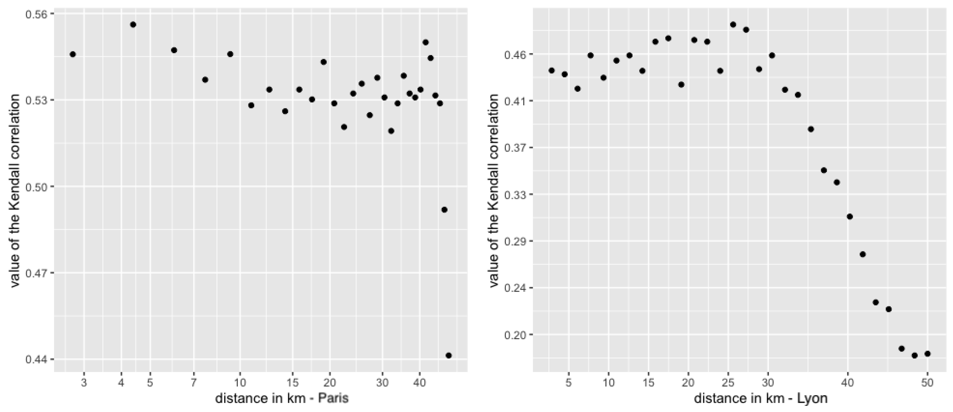
In a first exploratory part, we wanted to explore the distance from the cemetery to consider for establishing the link between the CHIMERE Cd atmospheric forecasts and the Cd measurements in mosses. We had one CHIMERE forecast for a squared zone of 3 km × 3 km, not a forecast at each cemetery site. Moreover, we did not know a priori the influence of reasonably far atmospheric metals on a cemetery site. Therefore, from each cemetery, we established different circular zones with a
d radius, with the
d distance varying from
to 50 km, and in each zone we calculated the mean of all the CHIMERE forecasts (one unique forecast in the area with
km). Then, for each
d area, considering all cemeteries, we calculated the Kendall rank correlation between the measurements in mosses and the CHIMERE means attached to the
d area around each cemetery. Finally, we had a Kendall rank correlation by
d distance, and we could determine the distance that maximized the Kendall rank correlations between the CHIMERE forecasts and the measurements in mosses. The
R (
https://www.r-project.org/ (accessed on 13 April 2021)) package
allows to calculate these Kendall rank correlations.
2.4. Linear Models with Fixed Effects
When observing a linear link between two variables of interest (here Cd measurement in mosses and CHIMERE Cd forecast), it is natural to produce linear models with other known explanatory covariates to explore in depth the relation between both variables. Here, we chose to explain Cd in mosses by the CHIMERE forecast with other covariates collected at the time of the moss sampling, such as the altitude of the sampling site, A; the type of support on which the moss was taken, S; the presence or not of traces of a phytosanitary treatment, T; or the transect of sampling to which the moss belongs, r.
Starting model: in this model,
i indexes the mosses (
, for example, in Paris region). The
i’s are assumed independent and identically distributed. The starting model is the following:
where Cd is the Cd in the moss,
d is the distance from the data sampling center (as explained previously the cemeteries were chosen from a central site and the observed Cd concentrations seem decreasing with the distance from this center), and
is the CHIMERE Cd forecast mean from the 4 meshes around the cemetery
i. The
and
are here fixed effects depending on the sampling transects (8 sampling transects, see
Figure 1). In addition,
, where
denotes the measure of uncertainty (variance; the same for each
i moss).
Model selection: starting from this fairly rich model, one then proceeds to a selection of sub-models using the AIC criterion and a forward/backward method testing the sub-models [
29]. The
R function
allows one to estimate the models, calculate the AIC criterion, and perform the forward/backward method.
2.5. Linear Models with Random Effects
As an extension of the linear model with fixed effects, the random effect linear model introduces additional random sources of variability within the data [
30,
31]. In addition to moss measurement errors, there may occur some randomness stemming from the sampling of transects. These reported transects are only a sample of transects chosen among a population of the many other possible ones: variability between transects has to be introduced into the statistical analysis. Because of this between-transect diversity, correlation (due to similarities between mosses records at sites belonging to the same transect) is expected when grouping measurements by transect. Then, we can no longer suppose that moss data are independent as thought previously (in the linear model with fixed effects), but they are now independent only conditionally to the knowledge of the effect due to their transect belonging.
Starting model: in this model,
i indexes the mosses (
for Paris region and
for Lyon region). The
i’s are independent and are assumed to be identically distributed conditionally to their transect. The starting model is the following:
where Cd is the Cd in the moss and the covariates are the same than in the fixed effects linear model but here the
and
are random effects depending on the sampling transects (8 sampling transects as seen previously). Then,
where
denotes the measure of uncertainty of the mosses and
denotes the measure of uncertainty of the transects.
Model selection: starting from this fairly rich model, one then proceeds to a selection of sub-models using the AIC criterion and a forward/backward method testing the sub-models [
29]. The
R function
from package
allows us to estimate the models and calculate the AIC criteria for the forward/backward method.
2.6. Linear Models with Experimental Errors
We also had an additional information in the mosses data set: the experimental measurement error was provided by the laboratory that made the quantification of Cd in mosses. Two standard deviations of this error amount to 20% of the Cd value measured in each moss. Thus, the greater the measured value, the greater the uncertainty. We will therefore take into account this measurement error which can have a strong influence on the statistical fit.
Starting model: in this model, the
i’s are independent but are no longer assumed to be identically distributed: they have a variance proportional to the measurement error provided. The starting model is the following:
for
(Paris) and
(Lyon), where the same notations as previously are adopted. The
and
are here fixed effects because previous results did not justify the choice of a random model for them. In addition,
where
denotes the measurement error provided by the laboratory for the
i-th moss and
denotes the residual measure of uncertainty of the mosses.
Model selection: starting from this fairly rich model, one then proceeds to a selection of sub-models using the AIC criterion and a forward/backward method testing the sub-models [
29]. The
R package
allows to estimate the models and perform the forward/backward method testing the sub-models.
2.7. Linear Model with Chimere Errors
So far, we had considered the variable CHIMERE
as a deterministic explanatory quantity. However, remember that these data come from an interpolation of the meshes whose centers are close to the moss site. Indeed, we did not have CHIMERE data located at exactly the same points as the mosses but only a network of predictions that we had assumed to be uniform on each cell. In the following, we propose to interpolate the CHIMERE data at mosses points in another way, using two mathematical tools which are the variogram and the kriging [
32]. We therefore need to introduce a new uncertainty linked to the kriging estimation error.
As the previously introduced model selects the same variables whether for Lyon or Paris, we did not make a selection of sub-models but we relied on this same choice of covariates. Additionally, we will suppose that the Cd concentration CHIMERE
is itself a random process following at each point of Île-de-France and Lyon a normal law. We get the expectation (noted
) and the variance (noted
) of this process in each of the moss points (
for Paris) thanks to the kriging carried out at the moss points using the CHIMERE data. The regression problem is now written mathematically as follows:
where
is a value to estimate which allows a maximum of flexibility to the error uncertainty of each moss.
is still the measurement error provided by the laboratory for the
i-th moss.
Kriging at moss points: We started by constructing a variogram on the CHIMERE data. The empirical variogram was then fitted using a Matérn variogram model [
32]. We then used kriging at the blunt points (77 for Paris and 51 for Lyon). This kriging gave us at each of these points an average and a variance which therefore correspond to
and
, respectively.
Parameter estimation: As there was no predefined function in R to deal with this type of problem, we chose to solve the previous optimization problem “manually” by maximizing the log-likelihood. According to the model stated just above, marginally follows a normal distribution, . Moreover, the will be assumed to be independent, even if there is a small covariance between the . Therefore, the log-likelihood of the n-sample is given by
.
Dropping the constant term, this leads to
.
We then maximized this log-likelihood using the BFGS algorithm with the R package lbfgs. The value returned by this function corresponds to , where L denotes here the likelihood. The parameters were obtained at the end of this optimization. Their confidence intervals were obtained by bootstrap by fitting the model on 6000 samples obtained by drawing with replacement on data from mosses from the Paris and Lyon region.
2.8. Predictions at One City from a Model Fitted to the Other One
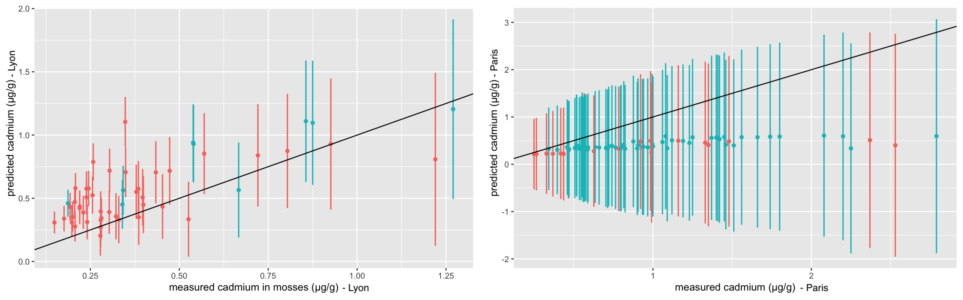
Finally, we wanted to explore the predictive value of the best founded model regarding the AIC criterion. For this, we calculated the moss measurements predictions at Lyon cemeteries from the best model fitted at Paris (we use the values of the Lyon covariates, the estimated values of the parameters from the model fitted at Paris and the model equation). Then, we compare those predictions with the observed measurements at Lyon to explore the predictive value of the best model. Furthermore, we did the same thing reversing the cities.
4. Discussion
The objectives of this study were to better understand the relationship between the atmospheric Cd concentrations modeled by CHIMERE in two French urban areas and Cd concentrations accumulated by mosses of the genus
Grimmia in the cemeteries of these two metropolitan areas. Although Paris is more densely populated than Lyon, the traffic is denser and the most emitting sites are located there, the two metropolises show similar average Cd concentrations (
Table 2), and a higher dispersion coefficient is found in Paris urban area (46%) than in Lyon urban area (41%). This global result is not surprising because the emission sources between the two cities are the same (energy transformation, road transport, and residential sector [
21]) but the size of studied area is different. Thus, for the Paris urban area, the study area includes more non-highly urbanized areas than the Lyon urban area. Nevertheless, the minimum and maximum values are higher in Paris than in Lyon. However, these values remain lower than those measured from PM in other European cities. For example, atmospheric Cd concentrations ranged from
to
g/m
in Warsaw in 2017 [
33] and were significantly lower than those measured in southern China (0.019
g/m
) [
34]. The authors of two recent studies used
Grimmia mosses as a passive bioaccumulator of metallic elements in the urban environment [
19,
20]. In our study, the concentrations of Cd accumulated by
Grimmia mosses are equivalent to those found by Gallego-Cartagena et al. in north Spain [
20] in sites under the influence of road traffic and industry, which could demonstrate that the origin of the contamination is atmospheric and not due to an effect of variables such as the substrate of mosses. The study carried out in Île-de-France did not analyze the Cd contents in mosses [
19], but demonstrated that
Grimmia pulvinata is a good proxy for atmospheric pollution by 20 elements (Al, As, Br, Ca, Ce, Cl, Cr, Cu, Fe, K, Mn, Ni, P, Pb, Rb, S, Sr, Ti, and Zn). This study highlights differences in the level of contamination in urban areas dependent on the distance from the urban environment [
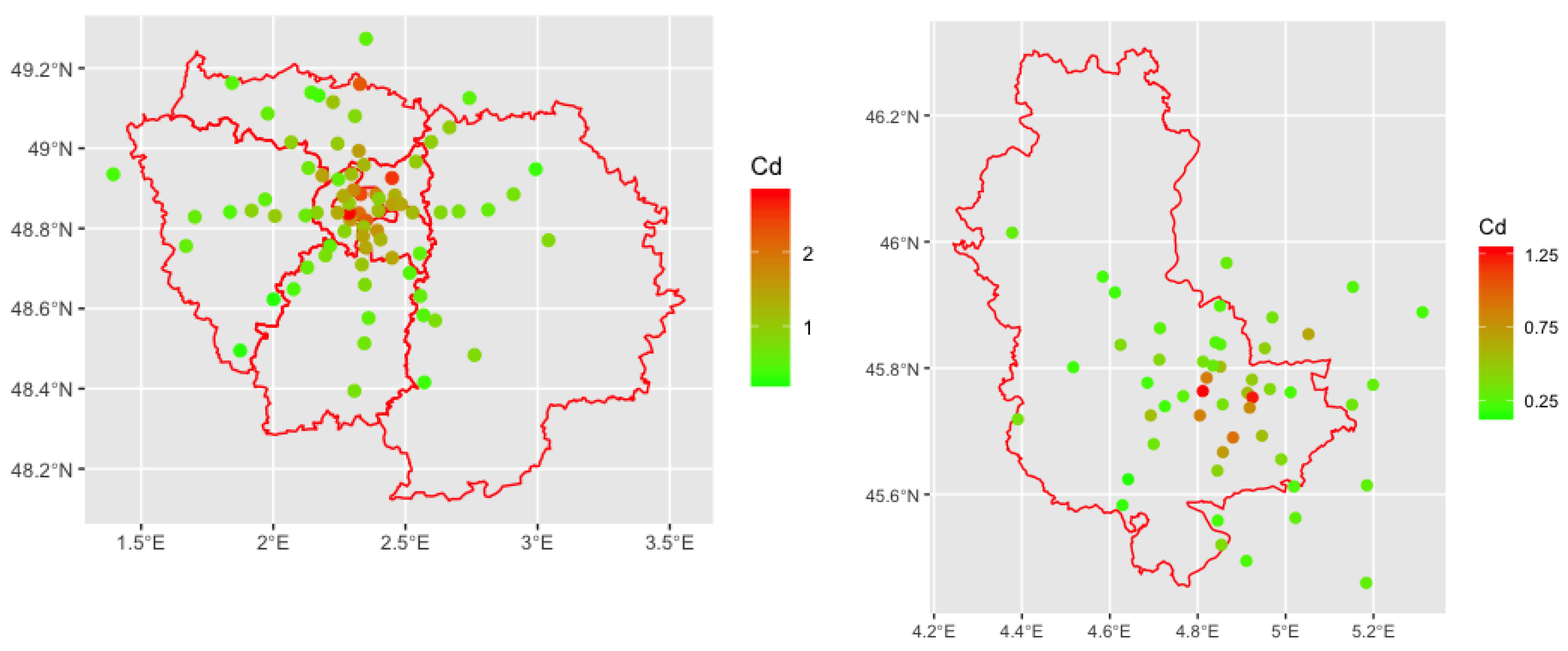
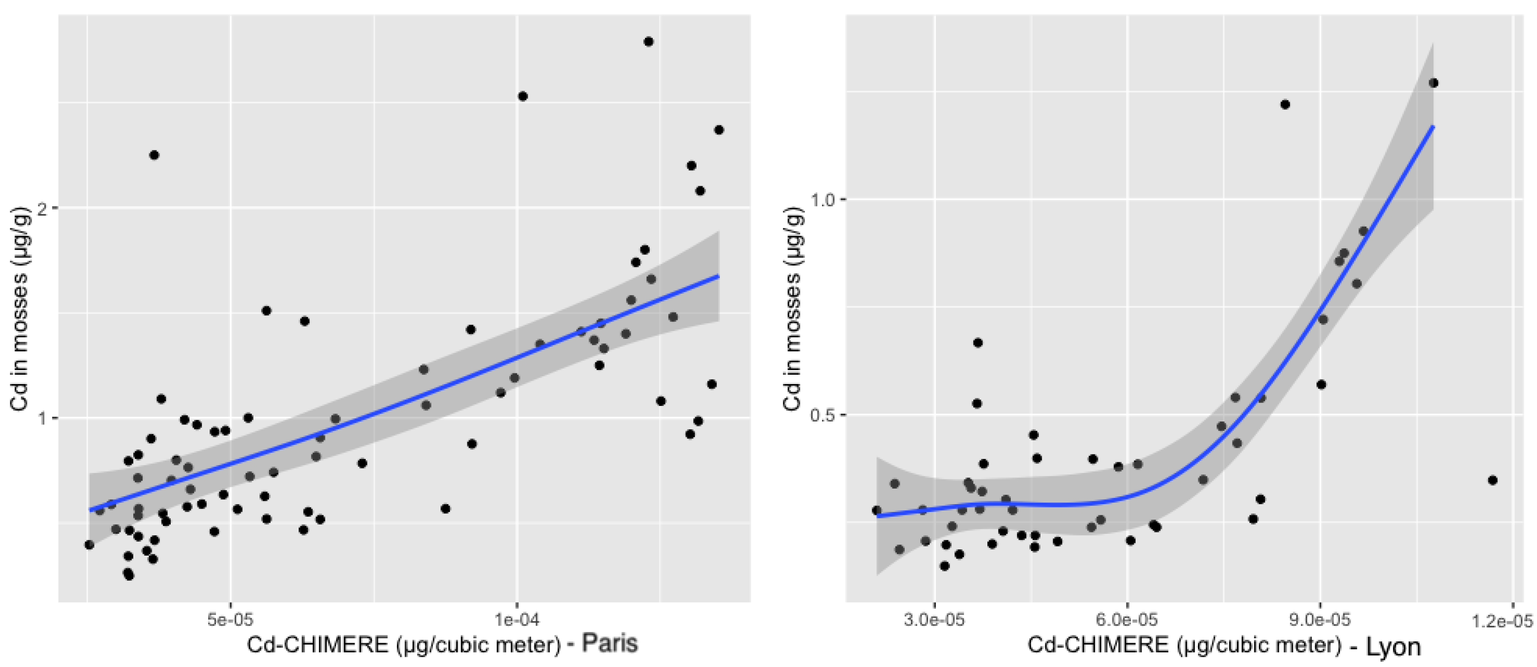
19]. Our mosses sampled in the cemeteries of the Paris and Lyon metropolitan areas have Cd contents which vary in the study area according to the atmospheric concentrations of Cd modeled by CHIMERE model. Our study makes it possible to add Cd to this list of elements studied in Île-de-France and makes it possible to specify that the variations of concentrations in the mosses are linked to the variations of concentrations in the atmosphere in two metropolitan areas of the territory.
Depending on the chosen spatial resolution, the Kendall correlations between the two series range between 0.44 and 0.56 for Paris metropolitan area and between 0.15 and 0.49 for Lyon metropolitan area. These rather weak correlations may stem from the fact that the available Cd atmospheric values simulated by the CHIMERE model date back to 2015, i.e., 3 years before the mosses were collected. However, the study of Cd emitted values since 1990 (from emission data compiled by European Monitoring and Evaluation Program (EMEP)) shows that they have remained stable since 2010. Moreover, to our knowledge, there is no other study on correlations between atmospheric Cd modeled on an urban area and the values of Cd concentrations in acrocarp mosses of the genus
Grimmia. Cd concentrations in mosses have previously been correlated with values of atmospheric deposition using EMEP transport models [
6,
7]. In these studies, the correlation values are significantly higher. Furthermore, Berg et al. [
35] and Berg and Steinnes [
36] find correlations of
0.82 – 0.84 between the Cd concentrations in
Hylocomium splendens and
Pleurozium schreberi and the wet deposits of Cd for mosses sampled as part of the European monitoring program. In mosses sampled in Europe in 2005/2006, Schröder et al. [
9] found a correlation of 0.65 between the Cd deposition of the sampling year and the concentrations in mosses and of 0.63 when considering the deposit over 3 years (Spearman correlations). This same study also showed that Cd concentrations in mosses were correlated with regional characteristics of the study area (urban land use at different radius).
Contrary to these studies, our results did not show a correlation between the Cd deposits modeled by CHIMERE near cemeteries and our Cd concentrations accumulated by
Grimmia in cemeteries (results not shown). These results could be explained by the fact that the atmospheric deposition calculated by CHIMERE in a mesh 3 km × 3 km relies on the main land use in the mesh and this main land use, in an urban area, must be hugely different from the land use in the cemeteries. This difference of land uses should evidently induce a discrepancy between the modeled deposition in the meshes and what is measured in the cemeteries. In Germany, Nickel et al. [
37] also demonstrated the importance of the deposition model taken into consideration in the correlations and showed a better correlation between modeled atmospheric deposition and Cd concentrations in mosses with deposit data modeled by LOTOS-EUROS which considers the land use, unlike deposits modeled by EMEP.
As for the studies carried out on mosses collected as part of the European monitoring program [
6,
9,
38], the values of Cd concentrations in mosses are correlated with the concentrations calculated in the atmosphere near cemeteries but, as in these studies, the atmospheric concentrations of Cd modeled cannot alone explain the Cd contents measured in our samples of
Grimmia. The values of Kendall correlations are lower in the metropolitan area of Lyon than in that of Paris and suggest that regional factors are involved in the relationship between atmospheric Cd and Cd accumulated by mosses [
13].
The various regression models fitted in this study allowed us to explore this relationship in more details. First, before taking into account the uncertainty associated with analytical measurement errors, the two types of adjusted models (fixed and random effects) show that altitude is one of the factors influencing the results in the Paris metropolitan area, as well as the sampling transects. However, once we consider the uncertainty related to the analytical measurement (20% of the measurement), the model has recourse to the same explanatory covariates for the two metropolitan areas, with AICs which suggest a clear improvement in the fit of the models. In addition to Cd CHIMERE forecasts, only the support on which moss was taken remains an explanatory variable in the model of the two cities.
Table 3 of the most complex model shows that the coefficient of this “support” variable is not significantly different between metropolitan areas. In our study, the concentrations of Cd accumulated by the mosses collected from the graves are higher than for the mosses collected from the walls of the cemetery. However, it is not possible to conclude with certainty on the origin of this difference in concentrations between mosses taken from graves and walls. Indeed, due to the religious character of the cemeteries and the number of graves and walls sampled, it was impossible to take samples from the graves’ substrates for analysis to crosscheck for diffusion. Nevertheless, a simple chemical analysis of the cement would not have provided a definitive answer because the essential factor is the bioavailability of the element in the substrate, and the metal content of the substrate is not indicative of the values found in mosses [
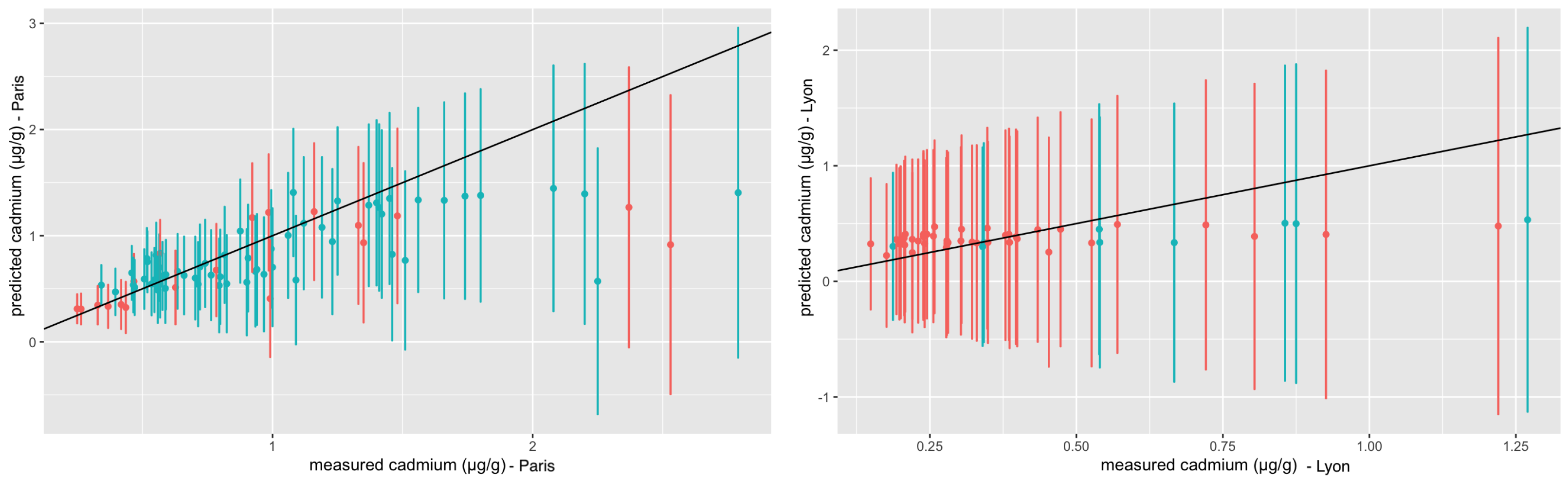
39]. This last model tested (linear model with experimental errors and CHIMERE errors) based on a kriging, i.e., a linear combination of all the surrounding CHIMERE cells whose coefficients are the correlations with the cemetery, still allows a decrease in AIC and therefore even better overall adjustment in Paris and Lyon metropolitan areas. This more complex consideration of the CHIMERE data and their error makes it possible to take better account of the fact that these data are imprecise at the mosses sampling coordinates because they are evaluated at another geographical scale and the model is less accurate for high values of Cd (
Figure 7). In the Lyon metropolitan area, some average predictions are far apart from those measured, but the intervals of uncertainties are important and the model is reliable. Yet,
Table 3 shows that the slope of the CHIMERE variable is significantly different in the two metropolitan areas, thus reflecting a regional effect of the atmospheric Cd concentration. Therefore,
Figure 8 shows that the two models are not reliable to be transposed to the other region. Further investigations should be performed to understand whether the introduction of regional effects could permit substantial improvements in fitting and in predictive use of such models.
5. Conclusions
Mosses of the genus Grimmia are efficient Cd bioaccumulators in urban and peri-urban environments and can be used as a proxy for atmospheric Cd concentrations. For the first time, our results show that the Cd concentrations in acrocarpous mosses are correlated with the modeled Cd concentrations by the CHIMERE chemistry transport model in two French metropolitan areas: Paris and Lyon. The better model is a linear model with experimental errors and CHIMERE errors based on a kriging and including the variable “substrate of moss sampling”. The relationships between Cd concentrations in mosses and modeled Cd concentrations by the CHIMERE depend on some regional factors and the model developed for one metropolitan area is not fully reliable to predict the Cd observations of the other metropolitan area.
Despite the large difference in the coefficients of the model adjusted to Lyon or Paris, we obtain a consistent prediction of the level of cadmium present in the moss. However, in addition to the difference in coefficients between the two cities, it seems reasonable to think that this model can only be applied to large cities, where cadmium pollution is quite high, as is the case for Lyon and Paris. In rural areas, for example, initial investigations led us to believe that there was no such link on this scale. Studies in other urban and peri-urban areas would provide a better understanding of the regional variability of the models. Finally, it would be interesting to develop similar models for other elements modeled by CHIMERE and analyzed in our moss samples such as As, Ni, and Hg.


 ,
, 


