On the u_⋆−U Relationship in the Stable Atmospheric Boundary Layer over Arctic Sea Ice

Abstract

A relationship between the friction velocity $u_{\star }$ and mean wind speed U in a stable atmospheric boundary layer (ABL) over Arctic sea ice was considered. To that aim, the observations collected during the Surface Heat Budget of the Arctic Ocean (SHEBA) experiment were used. The observations showed the so-called “hockey-stick” shape of the $u_{\star }-U$ relationship, which consists of a slow increase of $u_{\star }$ with increasing wind speed for $U<U_{tr}$ and a more rapid almost linear increase of $u_{\star }$ for $U>U_{tr}$, where $U_{tr}$ is the wind speed of transition between the two regimes. Such a relationship is most pronounced at the highest observational levels, namely at 9 and 14 m, and is also sharper when the air-surface temperature difference exceeds its average values for stable conditions. It is shown that the Monin–Obukhov similarity theory (MOST) reproduces the observed $u_{\star }-U$ relationship rather well. This suggests that at least for the SHEBA dataset, there is no contradiction between MOST and the “hockey-stick” shape of the $u_{\star }-U$ relationship. However, the SHEBA data, as well as the single-column simulations show that for cases with strong stability, $u_{\star }$ significantly decreases with height due to the shallowness of the ABL. It was shown that when $u_{\star }$ was assumed independent of height, the value of the normalized drag coefficient, i.e., of the so-called stability correction function for momentum, calculated using observations at a certain level, can be significantly underestimated. To overcome this, the decrease of $u_{\star }$ with height was taken into account in the framework of MOST using local scaling instead of the scaling with surface fluxes. Using such an extended MOST brought the estimates of the normalized drag coefficient closer to the Businger–Dyer relation.

1. Introduction

Turbulent heat and momentum exchange are the key processes carrying out thermodynamic coupling among the atmosphere, sea ice, and ocean in the Arctic and, thus, have to be adequately parameterized in numerical climate and weather prediction models [1]. The Arctic atmospheric boundary layer is different from that in lower latitudes due to the frequent occurrence of the so-called long-lived stable stratification in the lower atmosphere [2], which is formed due to the radiative cooling of the surface and of the atmosphere during polar night [3].

Typically, at least two regimes are identified in a stable atmospheric boundary layer (ABL): the weakly stable and the strongly stable ones [4,5] with a sharp transition between them [3,6].

It is generally accepted that for weakly stable stratification, Monin–Obukhov similarity theory (MOST) describes the nondimensional properties of the surface layer well. Furthermore, MOST based on local scaling was shown to be valid for heights above the surface layer in a stable ABL within a large stability range using both observations [7,8] and large eddy simulations [9].

However, recently, it was proposed by Sun et al. [10,11,12] that even for weak stability, in a nearly neutral nocturnal ABL, MOST is valid only within the few lowest meters. In particular, using the Cooperative Atmospheric Surface Exchange Study (CASES-99) data, Sun et al. considered in detail the relationship between the friction velocity $u_{\star }={[{\left(\overline{u^{\prime }{w}^{\prime }}\right)}^2+{\left(\overline{v^{\prime }{w}^{\prime }}\right)}^2]}^{0.25}$ and the mean wind speed U. In the CASES-99 data, such a relationship resembles a “hockey stick” (see Figures 4 and 8 in Sun et al. [11]): for weak wind, $u_{\star }$ almost does not grow with increasing U, while for U larger than some transitional value $U_{tr}$, $u_{\star }$ increases almost linearly with U. Sun et al. suggested that the “hockey-stick” behavior is associated with a transition from a regime of turbulence suppressed by stability (weak wind) to a well-mixed regime where large eddies with scales larger than z play a significant role in the momentum exchange [11].

In particular, for the near-neutral conditions during night, Sun et al. [11] obtained a dependency:

$$u_{\star }\left(z\right)=\alpha \left(z\right)U\left(z\right)+\beta \left(z\right),$$

(1)

where the coefficients $\alpha$ and $\beta$ are functions of the observational height z with $b\left(z\right)<0$ for a nocturnal ABL.

Sun et al. [11] noted that Equation (1) deviates from the $u_{\star }-U$ relationship, which follows from the logarithmic wind profile, namely:

$$u_{\star 0}=C_d^{1/2}U\left(z\right),$$

(2)

where the drag coefficient is given by

$$C_d=\frac{k^2}{{\left(\ln [z/z_0]\right)}^2}.$$

(3)

In (3), $u_{\star 0}$ is the friction velocity at the surface, $k=0.4$ is the von Karman constant, z is the height of observations in the surface layer, and $z_0$ is the roughness length for momentum.

Sun et al. [11], as well as Grisogono et al. [13] argued that the deviation of the observed $u_{\star }-U$ relationship (1) from (2) points to the weakness of MOST even for the near-neutral stratification. At the same time, Chenge and Brutsaert [14] showed that the the flux-profile relationships during CASES-99 are in agreement with MOST for stable stratification. Thus, it remains unclear whether the “hockey-stick” shape of the $u_{\star }-U$ relationship points to the breakdown of MOST. Thus, the main focus of this paper was to resolve this controversy.

The first goal of this paper was to investigate whether the “hockey-stick” behavior is present in the most comprehensive dataset over the Arctic sea ice, namely the one obtained during the Surface Heat Budget of the Arctic Ocean experiment (SHEBA) [15]). The second goal was to show whether the observed $u_{\star }-U$ relationship can be obtained in the framework of MOST. To that aim, the classical surface layer MOST, as well as a single-column RANS model were used to reproduce the $u_{\star }-U$ relationship as observed at SHEBA in winter.

It is important to note that the region of applicability of MOST for the SHEBA dataset was already studied earlier by Grachev et al. [16] and Grachev et al. [17]. In particular, Grachev et al. [16] found that in stable conditions already for $z/L>1$, where L is the Obukhov length, local scaling was more appropriate than the surface scaling. Moreover, for strongly stable cases, a significant Ekman turning of wind was observed in the lowest 20 m. This shows that the ABL over sea ice can be very shallow and the classical surface layer assumptions can be violated even at low observational heights.

This motivated us to explore if the decrease of $u_{\star }$ with height affects the $u_{\star }-U$ relationship, as well as the estimations of the drag coefficient based on the observations at a given height. An approach to take such a decrease into account within MOST by using local scaling is presented and applied to the analysis of the SHEBA data.

2. Observations and Models

2.1. SHEBA Observations

In this study, the observations from the 20 m main SHEBA tower were used. The SHEBA ice camp is located at an ice floe, which drifted in the Beaufort and Chukchi Seas from October 1997 to October 1998. Here, we considered the polar night period from November 1997 to February 1998 when the frequency of stable conditions was the highest. During the winter, mean meteorological data and turbulent fluxes were measured at five levels located at 2.2, 3.2, 5.1, 8.9, and 14 m above the snow surface level. The exact heights slightly changed throughout winter due to the accumulation/melt of snow. At each level, the mean air temperature and humidity were measured using a Vaisala temperature and relative humidity probes. Three wind components were measured at 10 Hz at each level using sonic anemometers. We used the processed turbulence data available at https://data.eol.ucar.edu/dataset/13.114, accessed on 20 February 2021. [18]. This dataset contains the hourly values of turbulence statistics obtained using frequency integration of the turbulence spectra and cospectra. The processing details and the quality check procedures can be found in [19]. From the SHEBA dataset, also the snow surface temperature was used. It was estimated using the upwelling and downwelling longwave radiation and assuming the snow emissivity equal to 0.99 [19]. For the analysis, only the period when the net longwave radiative flux was lower than −20 Wm${}^{-2}$ was selected, which typically corresponds to clear-sky conditions.The reason for such a selection was that the negative longwave radiative balance leads to surface cooling and to the formation of a stable boundary layer. After the selection, the analyzed dataset consisted of about 800 data points (hourly averaged fluxes and mean parameters) for each observational level, while for the whole November-February period, the record contained about 1600 values for each level. Thus, in roughly half of the cases, the net longwave radiative flux was strongly negative. This resulted from the often observed bimodal distribution of the net longwave radiative flux and of the cloud fraction over the Central Arctic with clear-sky and opaque states being most frequent [20,21].

2.2. Surface-Layer MOST

According to MOST, the nondimensional wind speed gradient is:

$$\frac{kz}{u_{\star 0}}\frac{\partial U}{\partial z}={\varphi }_m\left(\frac{z}{L_0}\right).$$

(4)

In (4), ${\varphi }_m\left(z/L_0\right)$ is the universal function of the stability parameter $\zeta =z/L_0$ for momentum. The index “0” in $u_{\star 0}$ and $L_0$ indicates that the surface values of the fluxes are used in the definition of both. The Obukhov length $L_0$ is given by:

$$L_0=-\frac{{\theta }_{v0}{u}_{\star 0}^3}{kg{Q}_{vo}},$$

(5)

where ${\theta }_{v0}$ is the reference virtual potential temperature and $Q_{v0}$ is the kinematic virtual potential temperature flux at the surface. Over sea ice in the winter, the latter is very close to the kinematic temperature flux, namely $Q_{v0}\approx \left(\overline{w^{\prime }{\theta }^{\prime }}\right)=u_{\star 0}{\theta }_{\star 0}$, where ${\theta }_{\star 0}$ is the temperature scale.

Integrating (4) from $z_0$ to z, one obtains:

$$U\left(z\right)=\frac{u_{\star 0}}{k}\left[\ln \left(\frac{z}{z_0}\right)-{\mathsf{\Psi }}_m\left(\frac{z}{L_0}\right)+{\mathsf{\Psi }}_m\left(\frac{z_0}{L_0}\right)\right],$$

(6)

where ${\mathsf{\Psi }}_m(z/L_0)$ is the stability function for momentum.

A number of stability functions were proposed for stable stratification (e.g., [22]). Here, we used the so-called Businger–Dyer stability functions [23,24], namely:

$${\mathsf{\Psi }}_m=-5\frac{z}{L_0},$$

(7)

as well as the more complex nonlinear SHEBA stability functions [25].

2.3. Single-Column RANS Model

A simple single-column atmospheric model coupled to an ice-snow model was used in this study. The atmospheric model consisted of the prognostic equations for the horizontal wind components and potential temperature, namely:

$$\begin{array}{ccc}\hfill \frac{\partial U}{\partial t}& =& f(V-V_g)-\frac{\partial \left(\overline{u^{\prime }{w}^{\prime }}\right)}{\partial z},\hfill \end{array}$$

(8)

$$\begin{array}{ccc}\hfill \frac{\partial V}{\partial t}& =& -f(U-U_g)-\frac{\partial \left(\overline{u^{\prime }{w}^{\prime }}\right)}{\partial z},\hfill \end{array}$$

(9)

$$\begin{array}{ccc}\hfill \frac{\partial \theta }{\partial t}& =& -\frac{\partial \left(\overline{w^{\prime }{\theta }^{\prime }}\right)}{\partial z}-\frac{\partial F_{LW}}{\partial z},\hfill \end{array}$$

(10)

where $U_g$ and $V_g$ are the geostrophic wind components, f is the Coriolis parameter, and $F_{LW}$ is the longwave radiative flux. Condensation, as well as the shortwave radiative heating were neglected because the focus was on clear-sky conditions during polar night, which promote stable atmospheric boundary layer formation. Relative humidity in the whole atmospheric column was assumed to be 80% with respect to the saturation over ice. Horizontal advection and subsidence were also neglected for simplicity.

A first-order local closure was used to parameterize turbulent fluxes of heat and momentum as:

$$\begin{array}{ccc}\hfill \overline{w^{\prime }{\theta }^{\prime }}& =& -K_H\frac{\partial \theta }{\partial z},\hfill \end{array}$$

(11)

$$\begin{array}{ccc}\hfill \overline{u^{\prime }{w}^{\prime }}& =& -K_M\frac{\partial u}{\partial z},\hfill \end{array}$$

(12)

$$\begin{array}{ccc}\hfill \overline{v^{\prime }{w}^{\prime }}& =& -K_M\frac{\partial v}{\partial z},\hfill \end{array}$$

(13)

where the eddy diffusivities are given by:

$$\begin{array}{ccc}\hfill K_M& =& \left|\frac{\partial \mathbf{V}}{\partial z}\right|l^{2}f\left(Ri\right),\hfill \end{array}$$

(14)

$$\begin{array}{ccc}\hfill K_H& =& K_M.\hfill \end{array}$$

(15)

In (14), l represents the mixing length scale for which the Blackadar formula is used:

$$l=\frac{kz}{1+kz/\lambda },$$

(16)

where $\lambda$ is the maximum mixing length in the boundary layer. In our study, we used $\lambda =30$ m, similar to Vihma et al. [26]. More physically justified expressions for $\lambda$ exist (e.g., [27]), but using them did not lead to qualitatively different results.

The effect of stratification on $K_{M,H}$ was taken into account by using the stability function $f\left(Ri\right)$ in (14) where $Ri$ is the gradient Richardson number. For stable conditions, we used:

$$f\left(Ri\right)=\left\{\begin{array}{cc}\max \left[0.005,{(1-5Ri)}^2\right];\hfill & Ri<0.2\hfill \\ 0.005;\hfill & Ri\ge 0.2,\hfill \end{array}\right.$$

(17)

which is the Richardson number equivalent of the Businger–Dyer stability functions [28]. The limit $0.005$ was introduced to represent some small level of background turbulence, which is often present due to processes not taken into account explicitly, such as braking gravity waves and sub-mesoscale non-stationary motions. The value 0.005 was not derived theoretically, but was close to the values suggested by observations [14] and sensitivity studies [29]. Such a closure was successfully used in Vihma et al. [26] to simulate the stable ABL development during warm-air advection over ice. The model in this setup also agreed well with the GABLS I large-eddy simulations of a stable ABL [30] (not shown here).

In the surface layer, the turbulent fluxes of heat and momentum were parameterized using Monin–Obukhov similarity theory. The roughness length for momentum was set to $z_0=3.3\times {10}^{-4}$ m, which is the average value for SHEBA [31]. For the roughness length for scalars, we used $z_{0t}=0.1z_{0m}$. The longwave radiative flux $F_{LW}$ was calculated using the Goddard longwave radiative transfer model [32].

The snow/ice model is represented by the heat diffusion equation:

$${\rho }_{i,s}c\frac{\partial T_{i,s}}{\partial t}=k_{i,s}\frac{{\partial }^2{T}_{i,s}}{\partial z^2},$$

(18)

where $k_{i,s}$ are the thermal conductivities for ice and snow (2.2 and 0.21 W m${}^{-1}$K${}^{-1}$, respectively), ${\rho }_{i,s}$ are the ice and snow densities (916 and 290 kg m${}^{-3}$, respectively), and $c=2100$ J kg${}^{-1}$K${}^{-1}$ is the specific heat capacity of ice. At the lower ice boundary, the sea ice temperature was set to the freezing temperature of saline water (271.15 K). At the upper boundary, the snow temperature was found as a solution of the heat balance equation at the snow surface. Sea ice and snow thickness were constant (2 and 0.3 m, respectively) throughout the simulation.

A constant vertical grid-spacing of 2 m was used in the atmosphere, which is sufficient to resolve shallow boundary layers. The height of the lowest level was 1 m. The top of the model domain was located at 2400 m, as we were interested in the lower atmosphere.

The model was forced by prescribing various values of the geostrophic wind and was integrated over 24 h. The initial temperature profile was typical for the Arctic and was based on the radiosounding obtained at the Russian drifting station “North Pole-37” (Figure 2 in [3]). The described model with a similar setup was used earlier to simulate clear-sky cooling over the Arctic sea ice in the presence/absence of leads [3].

Models of a similar complexity were shown to reproduce a stable ABL over sea ice/snow rather well given that the vertical resolution was sufficient (e.g., [30,33]). However, the limitations of the idealized setup and the simplicity of the model should be clearly understood. Taking into account additional physics, such as the nonstationarity of the forcing, surface heterogeneity, and large-scale subsidence [34], would bring more realism to the simulations. While here, preference was given to simplicity, the obtained results can be refined in the future using more complex models and simulation scenarios.

3. Results

3.1. Observations

Typically, the turbulent properties of the surface layer are presented as functions of the stability parameters, such as $z/L$ and bulk, gradient, and flux Richardson numbers. This has been done for the SHEBA dataset in a number of studies [22,25,35]. A different approach is to relate the turbulence velocities to the mean flow properties [10,36]. We followed the second approach using $u_{\star }$ as one of the turbulence velocities.

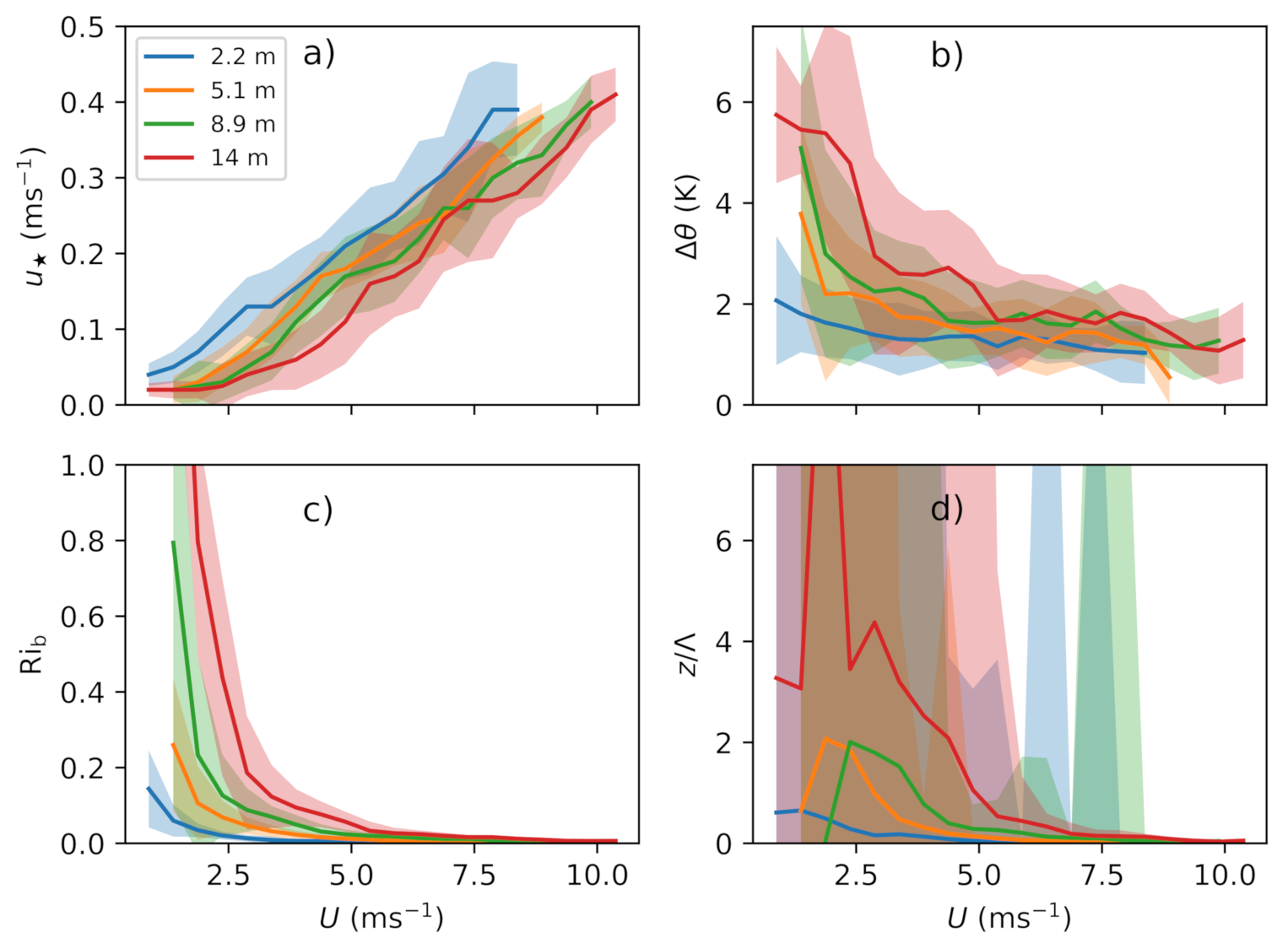
Figure 1a shows the observed $u_{\star }$ as a function of mean wind speed U at four levels of the SHEBA mast. Only the observations at 2.2, 5.1, 8.9, and 14 m are shown, while the 3.2 m level was skipped in order not to overload the figures. The curves represent median values of $u_{\star }$ obtained for the regular intervals of U. The intervals are 1 ms${}^{-1}$ wide. Obviously, the “hockey-stick” shape of the $u_{\star }-U$ relationship starts to be visible at higher levels. It is especially pronounced at 14 m, where $u_{\star }$ is nearly constant and close to zero for $U<3$ ms${}^{-1}$ and increases quasi-linearly with U for $U>3$ ms${}^{-1}$. The transitional value of wind speed $U_{tr}$ is larger for higher observational levels, which was in agreement with the CASES-99 [10] and Cabauw observations [4].

It can be seen from Figure 1b that when U decreases, the potential temperature difference between air and surface $\mathsf{\Delta }\theta ={\theta }_a-{\theta }_s$ increases. Such an increase of $\mathsf{\Delta }\theta$ becomes especially rapid for $U=U_{tr}$ where $U_{tr}$ is the wind speed of transition between the strongly stable and weakly stable regimes. Thus, when U approaches $U_{tr}$, a jump-like increase of stability is evident from Figure 1c,d, both in terms of the bulk Richardson number $R{i}_b$ and $z/\mathsf{\Lambda }$, where $\mathsf{\Lambda }$ is the Obukhov length calculated using locally observed $u_{\star }$ and ${\theta }_{\star }$. For $U<U_{tr}$, the value of the bulk Richardson number ${\mathrm{Ri}}_{\mathrm{b}}$ exceeds 0.2–0.25 for levels 5.1–14 m, which is often considered as the critical value over which the Kolmogorov turbulence collapses [17]. This suggests that the height of a fully turbulent boundary layer becomes comparable to the observational height for $U<U_{tr}$. For $U>U_{tr}$, the strength of stability gradually decreases and approaches the near-neutral limit for strong wind. Thus, stability is expected to affect the nondimensional velocity profiles and turbulent transfer coefficients in a broad range of U, not only for $U<U_{tr}$. Furthermore, it is clear that both ${\mathrm{Ri}}_{\mathrm{b}}$ and $z/\mathsf{\Lambda }$ are larger for higher observational levels.

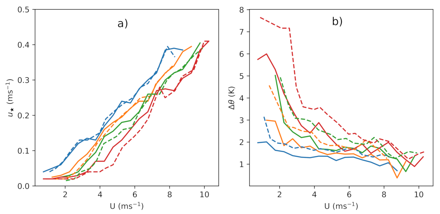
In order to highlight the effect of stratification on the $u_{\star }-U$ relationship, the cases when $\mathsf{\Delta }\theta$ (and hence, $R{i}_b$) exceeds its median value for each bin were selected. Figure 2 shows that the “hockey-stick” shape of the $u_{\star }-U$ relationship is even more pronounced for stronger stability and is visible already at a 5.1 m height. The increase of $\mathsf{\Delta }\theta$ leads to the increase of $U_{tr}$, especially at higher observational levels. The effect of the increased $\mathsf{\Delta }\theta$ is seen in a wide range of U, but becomes negligible for strong wind.

To summarize, the SHEBA observations show that the increase of stability for weak wind leads to a suppression of turbulence, and as a consequence, air becomes weakly coupled to the surface. From the surface heat budget point of view, at a low wind speed, the surface stops receiving heat via turbulent transfer, and this further increases $\mathsf{\Delta }\theta$ and stability. Such a positive feedback makes the regime transition especially abrupt. Moreover, for $U<U_{tr}$, the ABL height can become close to the observational level. This explains why $u_{\star }$ remains close to zero for $U<U_{tr}$. Such a regime transition mechanism was described earlier by Van de Wiel et al. [4,5] using the data from Cabauw, Netherlands, and Dome C, Antarctica, and by [3] for the Arctic boundary layer.

It is important to note that it is not the dimensional U that governs the regime transition. Concerning the $u_{\star }-U$ relationship, the appropriate nondimensional parameter is the bulk Richardson number, as shown further in Section 4. With respect to the $\mathsf{\Delta }\theta -U$, $R{i}_b-U$, and $z/L-U$ relationships, the suitable scaling can be introduced in a similar way as in [37] and [5]. In the latter, the velocity and temperature scales based on the net isothermal radiative flux were proposed.

Figure 1 also suggests that for strong wind and weak stability, i.e., for $U>U_{tr}$, the $u_{\star }-U$ relationship resembles Equation (1), which was proposed by Sun et al. [11] to describe the CASES-99 data. In the following subsection, it is discussed whether the classical MOST can reproduce such behavior.

3.2. Classical MOST Using Scaling with Surface Fluxes

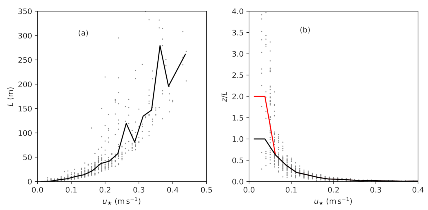
In this section, we present the $u_{\star }-U$ relationship as described by the classical MOST using scaling with surface fluxes (Equation (6)) for heights corresponding to the SHEBA observational levels. In order to use (6), one needs to specify the Obukhov length L as a function of $u_{\star }$ or U. To obtain L, the values of sensible heat flux observed at the lowest 2.2 m level at SHEBA were used. For the further calculations, the values of L were bin averaged for regular intervals of $u_{\star }$. The corresponding curves of L and $z/L$ as a function of $u_{\star }$ are shown in Figure 3. We set two limits for $z/L$ at $z=2.2$ m, namely $z/L\le 1$ and $z/L\le 2$. The first limit was applied when the Businger–Dyer stability functions were used in MOST and the second one when the SHEBA stability functions were used. This was done in order to avoid using Businger–Dyer stability functions outside their region of applicability, especially at higher observational levels.

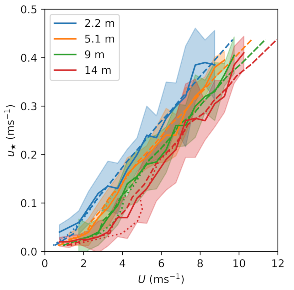
We assumed that $u_{\star }$ and L are independent of height and used the bin-averaged L in (6) to obtain U as a function of $u_{\star }$. Figure 4 shows the $u_{\star }-U$ relationships obtained using the Businger–Dyer and SHEBA universal functions for several observational heights. Obviously, the obtained curves were in close agreement with observations even though the values of L were prescribed in a rather simple manner. Closer examination of Figure 4 shows that using the SHEBA stability function in (6) resulted in a smoother decrease of $u_{\star }$ when U was decreasing. The Businger–Dyer stability function produced a more abrupt transition, which was especially pronounced at higher levels. This is a well-known feature of the Businger–Dyer functions, which were originally obtained for $z/L<1$ and do not allow for the turbulent exchange to persist for $R{i}_b\ge 0.2$. Although the presented results showed the sensitivity of the $u_{\star }-U$ relationship to using different stability functions, a thorough study of such a sensitivity is not in the scope of this paper.

It can be concluded that despite the fact that the observed $u_{\star }-U$ relationship had the “hockey-stick” shape, it was well reproduced by the classical MOST. The large difference between MOST and the “hockey-stick” shape as shown in the schematic Figure 1 in Grisogono et al. [13] was not identified. This suggested that the “hockey-stick” shape of the $u_{\star }-U$ relationship cannot be used to diagnose the breakdown of MOST, at least for the SHEBA data.

In the next section, the validity of the MOST assumptions of $u_{\star }$ and wind direction being constant with height is further addressed using the single-column model results.

3.3. Single-Column Modeling

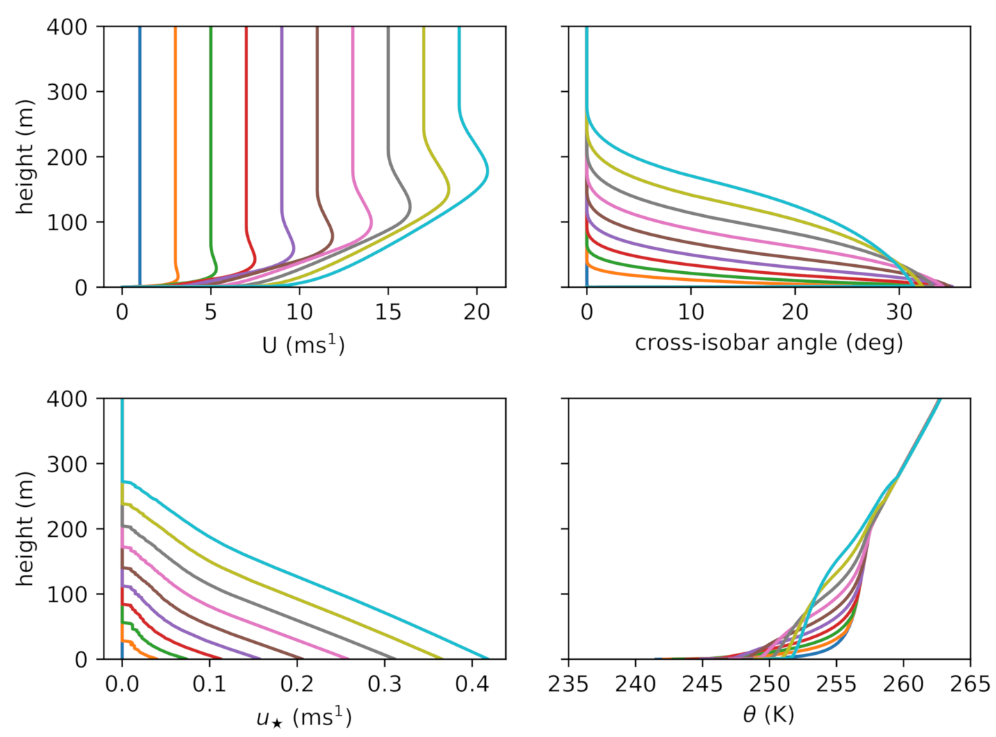
The results of the clear-sky cooling simulations using the single-column model are presented in Figure 5 for the moment of 24 h after the start of cooling. Figure 5 shows the vertical profiles of wind speed and direction, as well as of $u_{\star }$ and the potential temperature. The structure of the stable boundary layer over sea ice has already been considered in a number of idealized studies, which used the GABLS I scenario as a reference (e.g., [30,38,39,40]). The profiles shown in Figure 5 were in a good agreement with results obtained in the earlier studies, e.g., with respect to the ABL height and the surface cross-isobar angle, and will not be discussed here in much detail.

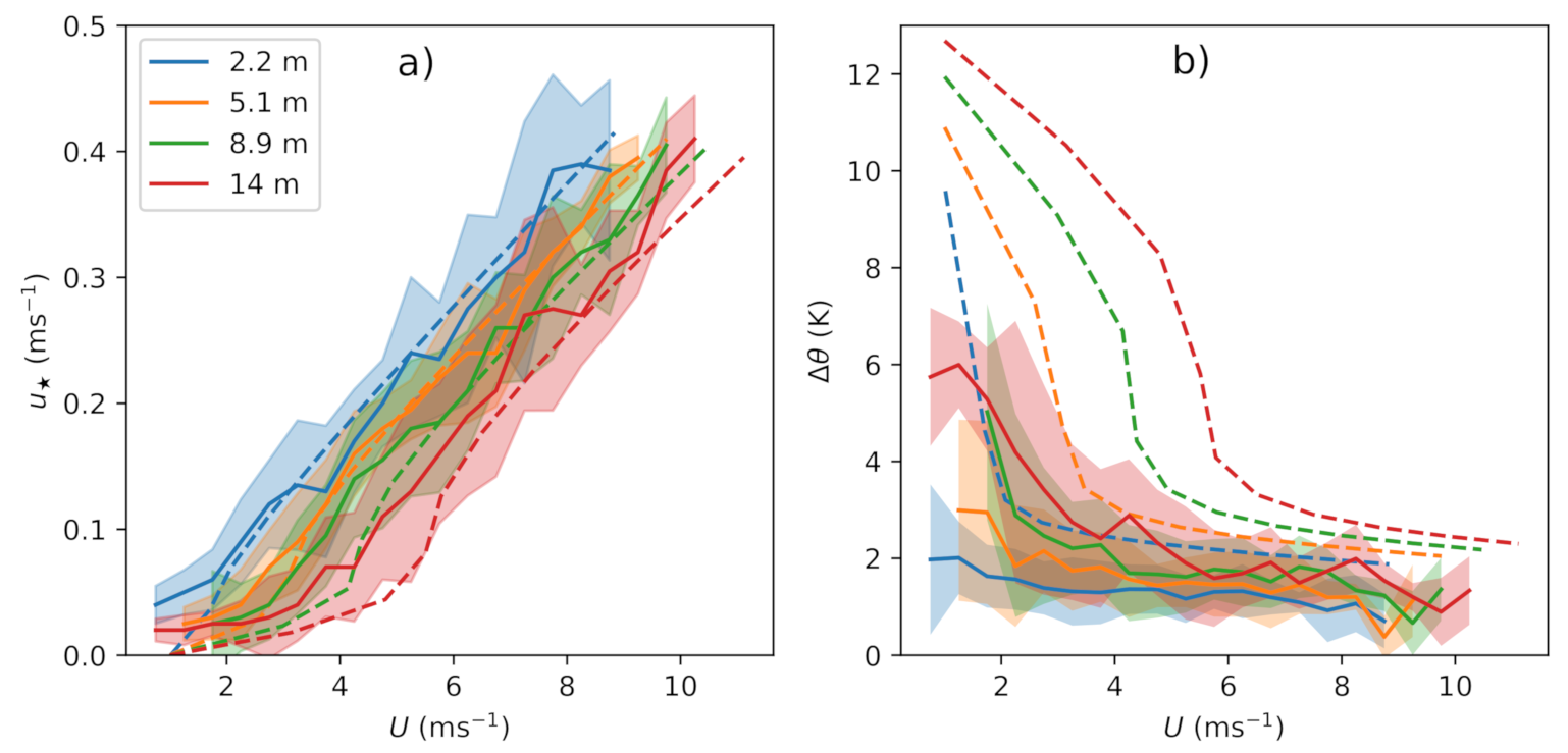
Figure 6 shows the comparison of the observed $u_{\star }-U$ relationship with the simulated one, as well as of the potential temperature difference ${\theta }_a-{\theta }_0$ as functions of wind speed. Clearly, the 1D model reproduced the “hockey-stick” shape of the $u_{\star }-U$ relationship, and a good agreement with observations was obtained. The simulated temperature difference was larger than in the observations. This showed that the simulations represented a rather intensive cooling scenario. This explained why the “hockey-stick” shape was more pronounced and $U_{tr}$ was larger in the single-column model results.

It should be noted that for $U<U_{tr}$, the observed $u_{\star }$ did not reach zero, but remained small positive. In contrast, in the single-column simulations, $u_{\star }$ approached zero, and this disagreement with observations was seen at all heights. This suggested that some level of the turbulence persisted even in weak wind conditions. Obviously, the used closure did not reproduce such a behavior even with the limit to the stability function. One possible way to take this into account in the model is to introduce explicitly the so-called minimum friction velocity. As shown by Grisogono et al. [13], this brought the $u_{\star }-U$ curves closer to the observed “hockey-stick” shape.

For this study, it was important that Figure 5 clearly shows that the ABL height decreased with decreasing wind speed and the ABL became shallower than 50 m already for the value of the geostrophic wind $U_g<5$ m s${}^{-1}$. Thus, one of the classical MOST assumptions, namely the condition $z\ll h$, where z is the typical height of the near-surface observations, e.g., the height of the SHEBA mast, was violated. One can expect that a decrease of $u_{\star }$ with height, as well as the wind turning can already be non-negligible at the height of observations. For the SHEBA data, this issue was investigated by Grachev et al. [16]. They showed that for $z/\mathsf{\Lambda }>1$, the vertical divergence of momentum flux increased and became non-negligible (their Figure 2). They also showed that for strong stability, the Ekman wind turning was observed at the observational levels.

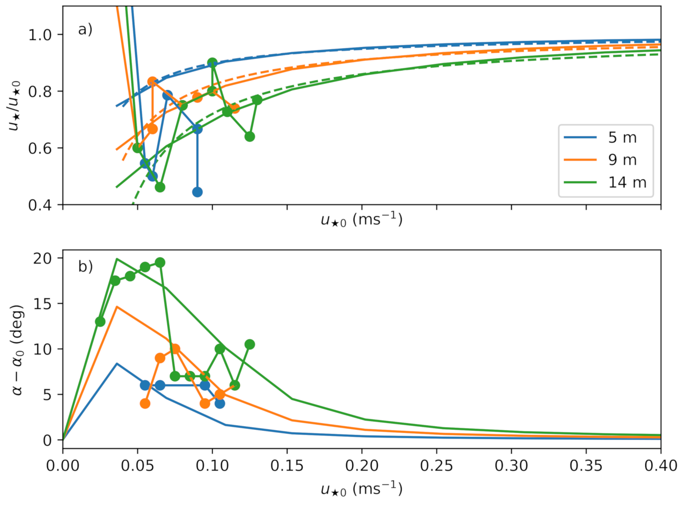
Figure 7a shows the ratio $u_{\star }/u_{\star 0}$ as a function of $u_{\star 0}$ where the latter is the surface value of $u_{\star }$, based on the model results and the SHEBA observations. The observations represented median values of $u_{\star }$ divided by the median values of $u_{\star 0}$ at the lowest level for regularly spaced bins of $u_{\star 0}$. Only those cases were considered when the local $z/\mathsf{\Lambda }$ exceeded one and when the observed $\mathsf{\Delta }\theta$ exceeded its median value for the given bin, i.e., cases with stronger stability. Figure 7a clearly shows that as $u_{\star 0}$ decreased, the decrease of $u_{\star }$ with height increased. Such a tendency was present both in the model results and in the observations, and both showed a similar magnitude of the decrease of $u_{\star }$ with height. Figure 7b shows that wind turning also increased as $u_{\star }$ decreased. It should be noted that the publicly available SHEBA dataset contains $u_{\star }$ values with the precision limited to only two digits after the decimal point. This might introduce additional scatter in the calculations of the vertical variation of $u_{\star }$, especially for low values of the latter. Thus, for a more detailed presentation of the $u_{\star }$ decrease with height, the reader is referred to Figure 2 in Grachev et al. [16].

This clearly showed that the ABL height h and the ratio $z/h$ had to be taken into account in the analysis of the $u_{\star }-U$ relationship in polar regions. A number of parameterizations for the height of a stable ABL were proposed in literature, which were reviewed by Zilitinkevich and Mironov [41], Zilitinkevich and Baklanov [42], and [43]. The most simple of them is the relation:

$$h=b{u}_{\star 0},$$

(19)

where $b=700$ s is the empirical constant whose value was obtained by [44] based on several datasets. Other parameterizations also resulted in a linear dependency of h upon $u_{\star }$ such as the ones by Rossby and Montgomery [45], Pollard et al. [46], and Kitaigorodskii and Joffre [47]. The difference of the mentioned parameterizations from Equation (19) is that they explicitly took into account the dependency of h on the Coriolis parameter f and the Brunt–Vaisala frequency N. Such parameterizations were based on dimensional analysis and suggested that b should be proportional to either $f^{-1}$, $N^{-1}$, or ${\left(fN\right)}^{-1/2}$.

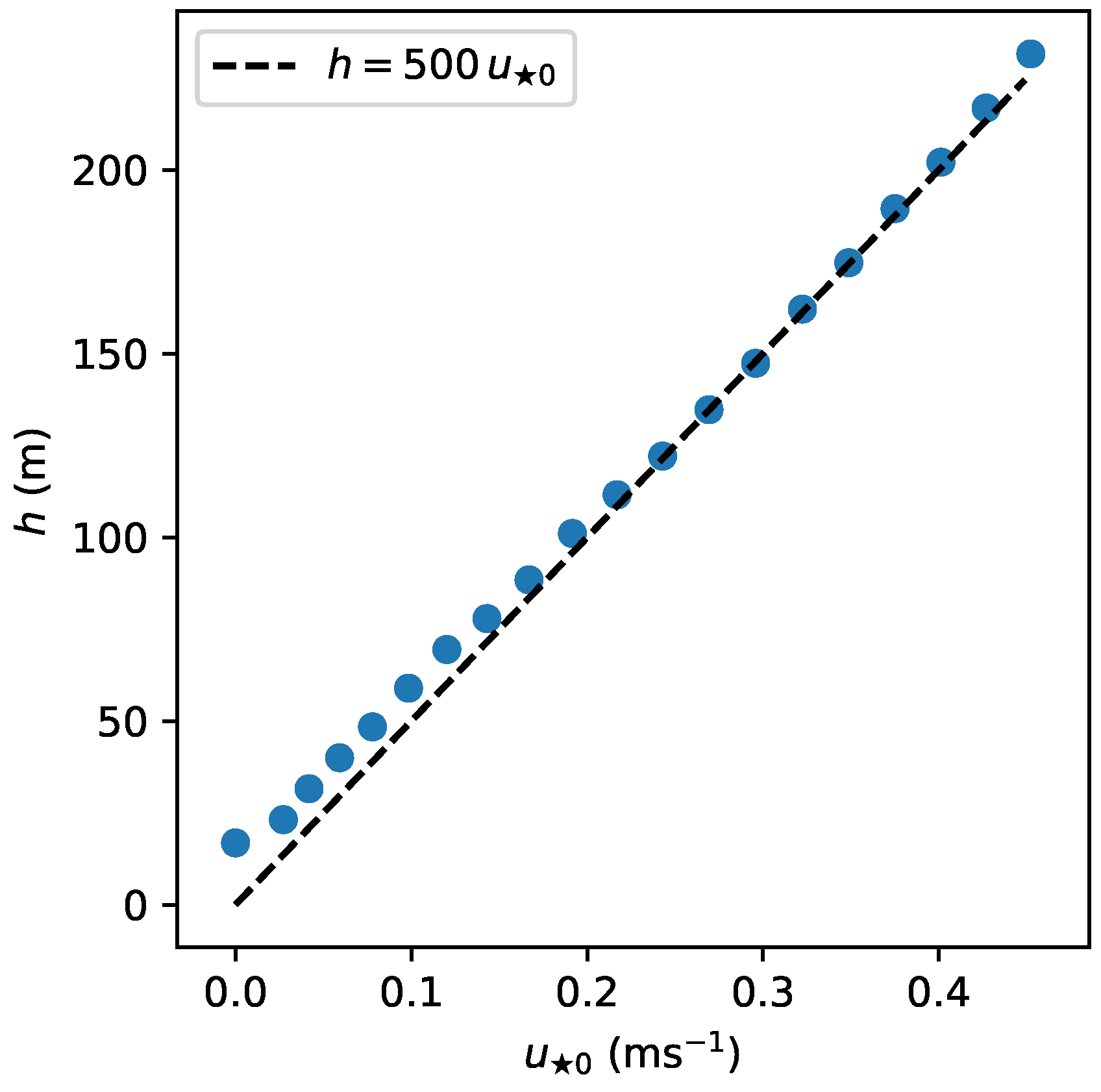
Figure 8 shows h as a function of $u_{\star 0}$ according to the single-column model simulations. The ABL height was diagnosed using $h=z^{\prime }/0.95$ where $z^{\prime }$ is the height where the vertical component of the turbulent momentum flux decreases to 5% of its surface value. Clearly, the obtained relationship was close to linear with $b=500$ s. The obtained value of b was smaller than the earlier proposed value of 700 s. This might be related to the idealized setup of the experiments and also to several factors that make the Arctic different from lower latitudes such as a stronger stability N, a larger Coriolis parameter f, and a smaller roughness $z_0$. A detailed study of the effect of these parameters on the ABL height is beyond the scope of this paper. We utilized Equation (19) as a simple practical solution.

Let us now assume a linear decrease of $u_{\star }$ with height, namely:

$$u_{\star }\left(z\right)=u_{\star 0}\left(1-\frac{z}{h}\right).$$

(20)

The dashed curve in Figure 7 was obtained using (Figure 8) in (20). The figure shows a good agreement of Equation (20) with the single-column model results. The parameterization (Figure 8) and (20) will be used in the following to reformulate the classical MOST using local scaling.

4. Extended MOST

Usually, MOST is associated with scaling with surface fluxes and the corresponding assumptions of $u_{\star }$ and ${\theta }_{\star }$ being constant with height. This results in the most simple practical application of MOST. However, MOST is not limited to the surface layer and is valid in a larger range of heights in the stable boundary layer when local scaling is used. An extension of the surface layer MOST towards local scaling can be obtained by allowing $u_{\star }$ and ${\theta }_{\star }$ to decrease with height. Such an extension of MOST is not novel and was used, for example, by Gryning et al. [48] to obtain the model for a wind profile in the whole ABL. Gryning et al. not only allowed $u_{\star }$ to decrease with height, but also introduced a combined mixing length scale. Here, we used a similar, yet simpler approach by allowing $u_{\star }$ and ${\theta }_{\star }$ to decrease linearly with height while keeping the length scale $kz$ unchanged.

We rewrite the classical MOST using Equation (20) as:

$$\frac{kz}{u_{\star 0}(1-z/h)}\frac{\partial U}{\partial z}={\varphi }_m\left(\frac{z}{\mathsf{\Lambda }}\right).$$

(21)

The local Obukhov length becomes:

$$\mathsf{\Lambda }=-\frac{{\theta }_0{u}_{\star 0}^2{(1-z/h)}^2}{kg{\theta }_{\star 0}(1-z/h)}=L_0(1-z/h).$$

(22)

Using the Businger–Dyer function ${\varphi }_m(z/\mathsf{\Lambda })=1+5z/\mathsf{\Lambda }$, we obtain:

$$\begin{array}{c}\hfill \frac{kz}{u_{\star 0}}\frac{\partial U}{\partial z}=1-\frac{z}{h}+5\frac{z}{L_0}.\end{array}$$

(23)

Note that (23) differs from the classical MOST only by the term $-z/h$ on the right-hand side.

Integrating (23) from $z_0$ to z, one obtains:

$$U=\frac{u_{\star 0}}{k}\left[\ln \frac{z}{z_0}-\frac{z-z_0}{h}+5\frac{z-z_0}{L_0}\right].$$

(24)

In the neutral limit, using (19) in (24), one obtains the following $u_{\star }-U$ relationship:

$$u_{\star }\left(z\right)=\frac{k}{\ln (z/z_0)}U\left(z\right)-\frac{z}{b}\left[1-\frac{1}{\ln (z/z_0)}\right]$$

(25)

It is interesting to note that (25) conforms to (1), which was obtained by Sun et al. [11] for the near-neutral and weakly stable conditions (for comparison of (25) with the log-law (2), see Appendix A). In the nocturnal ABL, Sun et al. [11] obtained negative values of $\beta \left(z\right)$ whose magnitude was increasing with height (their Figure 13). Equation (25) also suggested that $\beta \left(z\right)<0$ and its absolute value increased almost linearly with height, although being smaller than reported by Sun et al. [11].

The $u_{\star }-U$ relationship (24) provided by the extended MOST showed a similar agreement with the SHEBA data as the single-column model and the surface layer MOST (see the Appendix A). In the following, the difference between the surface layer and local formulation of MOST is discussed in more detail.

It is important to consider the effect of the modification of MOST on the transfer coefficient for momentum $C_d$. The latter is defined as:

$$C_d=\frac{u_{\star 0}^2}{U^2}.$$

(26)

Often, $C_d$ is represented as:

$$C_d=C_{dn}{f}_m$$

(27)

in order to separate the neutral part $C_{dn}$ and the so-called stability correction $f_m$ (also called the normalized transfer coefficient) (e.g., [22]). In frames of MOST, $f_m$ is a function of $z/L$ and $z/z_0$. It can also be expressed as a function of $R{i}_b$, $z/z_0$, and $z/z_t$. The presented extension of MOST introduces two more parameters $z/h$ and $z_0/h$ both in $C_{dn}$ and $f_m$, namely:

$$C_{dn}=\frac{k^2}{{\left[\ln (z/z_0)-(z-z_0)/h\right]}^2}$$

(28)

$$f_m={\left[1+\frac{5(z-z_0)/L_0}{\ln (z/z_0)-(z-z_0)/h}\right]}^{-2}$$

(29)

Using Businger–Dyer functions and assuming $z_t=z_0$, one obtains a simple relation between $z/L_0$ and $R{i}_b$ (e.g., [49]), namely:

$$\frac{z}{L_0}=\frac{R{i}_b\left[\ln (z/z_0)-(z-z_0)/h\right]}{1-5R{i}_b}.$$

(30)

Using (30) in (29) results in:

$$f_m={(1-5R{i}_b)}^2,$$

(31)

which is the same as in the classical MOST using scaling with surface fluxes. Thus, the drag coefficient in the classical and extended MOST differs only in $C_{dn}$ when the stability correction is approximated by (31). With $z=10$ m, $z_0=3.3\times {10}^{-4}$ m, and $z/h=0.5$, we obtained that $C_{dn}$ increased by about 10% as compared to the classical MOST. Thus, in the case when a bulk formula is used to calculate the surface momentum flux, our modification would result in a rather small increase of the latter. However, as shown further, a significant difference occurred in the interpretation of observations at a given height.

In order to further compare the extended MOST with the classical MOST, we used both to estimate the normalized drag coefficient $f_m=C_d/C_{dn}$ using observations of $u_{\star }$ and U at a given height. We used (27) as the definition of the drag coefficient. Within the classical MOST assumptions, $u_{\star 0}$ is simply equal to $u_{\star }$ at the height of observations. Within the extended MOST, we used (20) to obtain $u_{\star 0}$ from $u_{\star }$ observed at a given height. Neutral drag coefficient $C_{dn}$ was calculated using (28) for the extended MOST and using (3) for the classical MOST with $z_0=3.3\times {10}^{-4}$ m. The obtained $f_m$ is presented as function of $R{i}_b$ at a given observational level both for the classical and extended MOST.

We performed the $f_m$ calculations according to the described procedure using SHEBA observations and also the results of the single-column model simulations. The latter use Businger–Dyer stability functions, and therefore, we expected that using the assumptions of the extended MOST for the estimates of $f_m$ should result in a closer agreement of the obtained $f_m\left(R{i}_b\right)$ with (31). Figure 9 shows the resulting $f_m\left(R{i}_b\right)$ from the SHEBA data (a,b) and from the single-column model results (c,d). The black curve corresponds to (31) resulting from the Businger–Dyer universal functions. It is obvious that $f_m$ calculated assuming surface scaling were significantly below the Businger–Dyer curve both for the SHEBA and the model data. In frames of the extended MOST, the calculated $f_m$ agreed better with the Businger–Dyer curve for the SHEBA data although the scatter in $f_m$ increased. For the single-column model results, an excellent agreement with the Businger–Dyer function was obtained using the extended MOST, and the curves for different heights collapsed into one line.

Not that the curves of $f_m$ based on the model results did not approach zero for $R{i}_b\to 0.2$ because of the limit set on the stability function. When such a limit was not used, the obtained $f_m$ values reached zero for $R{i}_b=0.2$ (not shown here). A detailed analysis of the $f_m$ behavior for very strong stability is out of the scope of this paper, and the reader is referred to earlier studies [17,22].

The presented extension of MOST was expected to be valid only in the lower portion of the ABL, approximately for $z/h<0.5$. Such a limit of applicability could be extended following the approach in Gryning et al. [48], where a combined mixing-length scale was considered, and it was also assumed that U approaches the geostrophic wind speed for $z=h$. It should also be noted that the used linear decrease of $u_{\star }$ and ${\theta }_{\star }$ with height is an idealization, and other nonlinear dependencies have been proposed [48].

It is important to note that other universal functions, such as the SHEBA flux-profile relationships [25], can be used both within the classical and extended MOST. However, the integration procedure of such functions within the extended MOST framework might not be as straightforward as for the Businger–Dyer one.

5. Conclusions

The $u_{\star }-U$ relationship was studied using the SHEBA data over Arctic sea ice. Only the data during polar night and with sufficiently negative net longwave radiative flux were selected for the analysis. The “hockey-stick” shape of the $u_{\star }-U$ relationship was visible at higher observational levels (8.9 and 14 m) and became more pronounced when cases with increased air-surface temperature difference were selected.

It was shown that the $u_{\star }-U$ relationship obtained using the classical Monin–Obukhov similarity theory (MOST) based on scaling with surface fluxes was in a good agreement with the observed one. MOST reproduced also the “hockey-stick” shape rather well, at least for the SHEBA data. Such a good agreement was in contradiction with the schematic figure in Grisogono et al. [13] (their Figure 1) and suggested that the presence of the “hockey-stick” shape does not necessarily point to the weakness of the surface layer MOST.

Single-column simulations of a typical cooling scenario confirmed the findings by Grachev et al. [16] that the vertical divergence of the momentum flux can become significant, especially for the cases when the ABL height becomes shallow, i.e., at low wind speed. Furthermore, the single-column model results suggested the linear dependency of the stable ABL height on $u_{\star }$ at the surface.

These results were used to extend the classical MOST towards local scaling by allowing $u_{\star }$ and ${\theta }_{\star }$ to decrease linearly with height. This was done for the most simple Businger–Dyer universal functions. It was shown that using the local scaling led to a better agreement of the normalized drag coefficient $f_m\left(R{i}_b\right)$ calculated from observations with the Businger–Dyer relation. In contrast, surface scaling resulted in a significant underestimation of $f_m$. This was obtained both using the SHEBA observations and the single-column model results. Moreover, in the near-neutral limit, the extended MOST provided the $u_{\star }-U$ relationship, which conformed better to the linear expression approximating CASES-99 data.

To conclude, our results suggested that in the interpretation and analysis of observations in polar boundary layers, one has to take into account the decrease of $u_{\star }$ with height already at low observational heights.

References

- Vihma, T.; Pirazzini, R.; Fer, I.; Renfrew, I.A.; Sedlar, J.; Tjernström, M.; Lüpkes, C.; Nygård, T.; Notz, D.; Weiss, J.; et al. Advances in understanding and parameterization of small-scale physical processes in the marine Arctic climate system: A review. Atmos. Chem. Phys. 2014, 14, 9403–9450. [Google Scholar] [CrossRef] [Green Version]
- Zilitinkevich, S.S.; Esau, I.N. Resistance and heat-transfer laws for stable and neutral planetary boundary layers: Old theory advanced and re-evaluated. Q. J. R. Meteorol. Soc. 2005, 131, 1863–1892. [Google Scholar] [CrossRef] [Green Version]
- Chechin, D.G.; Makhotina, I.A.; Lüpkes, C.; Makshtas, A.P. Effect of Wind Speed and Leads on Clear-Sky Cooling over Arctic Sea Ice during Polar Night. J. Atmos. Sci. 2019, 76, 2481–2503. [Google Scholar] [CrossRef]
- De Wiel, B.J.H.V.; Moene, A.F.; Jonker, H.J.J.; Baas, P.; Basu, S.; Donda, J.M.M.; Sun, J.; Holtslag, A.A.M. The Minimum Wind Speed for Sustainable Turbulence in the Nocturnal Boundary Layer. J. Atmos. Sci. 2012, 69, 3116–3127. [Google Scholar] [CrossRef] [Green Version]
- De Wiel, B.J.H.V.; Vignon, E.; Baas, P.; van Hooijdonk, I.G.S.; van der Linden, S.J.A.; van Hooft, J.A.; Bosveld, F.C.; de Roode, S.R.; Moene, A.F.; Genthon, C. Regime Transitions in Near-Surface Temperature Inversions: A Conceptual Model. J. Atmos. Sci. 2017, 74, 1057–1073. [Google Scholar] [CrossRef] [Green Version]
- Vignon, E.; van de Wiel, B.J.H.; van Hooijdonk, I.G.S.; Genthon, C.; van der Linden, S.J.A.; van Hooft, J.A.; Baas, P.; Maurel, W.; Traullé, O.; Casasanta, G. Stable boundary layer regimes at Dome C, Antarctica: Observation and analysis. Q. J. R. Meteorol. Soc. 2017, 143, 1241–1253. [Google Scholar] [CrossRef]
- Nieuwstadt, F.T.M. The Turbulent Structure of the Stable, Nocturnal Boundary Layer. J. Atmos. Sci. 1984, 41, 2202–2216. [Google Scholar] [CrossRef]
- Nieuwstadt, F.T.M. Some aspects of the turbulent stable boundary layer. Bound.-Layer Meteorol. 1984, 30, 31–55. [Google Scholar] [CrossRef]
- Basu, S.; Porté-agel, F.; Foufoula-Georgiou, E.; Vinuesa, J.F.; Pahlow, M. Revisiting the Local Scaling Hypothesis in Stably Stratified Atmospheric Boundary-Layer Turbulence: An Integration of Field and Laboratory Measurements with Large-Eddy Simulations. Bound.-Layer Meteorol. 2006, 119, 473–500. [Google Scholar] [CrossRef] [Green Version]
- Sun, J.; Mahrt, L.; Banta, R.M.; Pichugina, Y.L. Turbulence Regimes and Turbulence Intermittency in the Stable Boundary Layer during CASES-99. J. Atmos. Sci. 2012, 69, 338–351. [Google Scholar] [CrossRef] [Green Version]
- Sun, J.; Lenschow, D.H.; LeMone, M.A.; Mahrt, L. The Role of Large-Coherent-Eddy Transport in the Atmospheric Surface Layer Based on CASES-99 Observations. Bound.-Layer Meteorol. 2016, 160, 83–111. [Google Scholar] [CrossRef]
- Sun, J.; Takle, E.S.; Acevedo, O.C. Understanding Physical Processes Represented by the Monin–Obukhov Bulk Formula for Momentum Transfer. Bound.-Layer Meteorol. 2020, 177, 69–95. [Google Scholar] [CrossRef]
- Grisogono, B.; Sun, J.; Belušić, D. A note on MOST and HOST for turbulence parametrization. Q. J. R. Meteorol. Soc. 2020, 146, 1991–1997. [Google Scholar] [CrossRef]
- Chenge, Y.; Brutsaert, W. Flux-profile Relationships for Wind Speed and Temperature in the Stable Atmospheric Boundary Layer. Bound.-Layer Meteorol. 2005, 114, 519–538. [Google Scholar] [CrossRef]
- Uttal, T.; Curry, J.A.; McPhee, M.G.; Perovich, D.K.; Moritz, R.E.; Maslanik, J.A.; Guest, P.S.; Stern, H.L.; Moore, J.A.; Turenne, R.; et al. Surface Heat Budget of the Arctic Ocean. Bull. Am. Meteorol. Soc. 2002, 83, 255–276. [Google Scholar] [CrossRef] [Green Version]
- Grachev, A.A.; Fairall, C.W.; Persson, P.O.G.; Andreas, E.L.; Guest, P.S. Stable Boundary-Layer Scaling Regimes: The Sheba Data. Bound.-Layer Meteorol. 2005, 116, 201–235. [Google Scholar] [CrossRef]
- Grachev, A.A.; Andreas, E.L.; Fairall, C.W.; Guest, P.S.; Persson, P.O.G. The Critical Richardson Number and Limits of Applicability of Local Similarity Theory in the Stable Boundary Layer. Bound.-Layer Meteorol. 2013, 147, 51–82. [Google Scholar] [CrossRef] [Green Version]
- Andreas, E.; Fairall, C.; Guest, P.; Persson, O. Tower, 5-Level Hourly Measurements Plus Radiometer and Surface Data at Met City (ASFG); Version 1.0; UCAR/NCAR-Earth Observing Laboratory: Boulder, CO, USA, 2007. [Google Scholar] [CrossRef]
- Persson, P.O.G.; Fairall, C.W.; Andreas, E.L.; Guest, P.S.; Perovich, D.K. Measurements near the Atmospheric Surface Flux Group tower at SHEBA: Near-surface conditions and surface energy budget. J. Geophys. Res. Ocean. 2002, 107, SHE 21-1–SHE 21-35. [Google Scholar] [CrossRef] [Green Version]
- Stramler, K.; Genio, A.D.D.; Rossow, W.B. Synoptically Driven Arctic Winter States. J. Clim. 2011, 24, 1747–1762. [Google Scholar] [CrossRef]
- Makhotina, I.A.; Makshtas, A.P.; Chechin, D.G. Meteorological winter conditions in the Central Arctic according to the drifting stations “North Pole 35–40”. IOP Conf. Ser. Earth Environ. Sci. 2019, 231, 012031. [Google Scholar] [CrossRef] [Green Version]
- Gryanik, V.M.; Lüpkes, C.; Grachev, A.; Sidorenko, D. New Modified and Extended Stability Functions for the Stable Boundary Layer based on SHEBA and Parametrizations of Bulk Transfer Coefficients for Climate Models. J. Atmos. Sci. 2020, 77, 2687–2716. [Google Scholar] [CrossRef]
- Businger, J.A.; Wyngaard, J.C.; Izumi, Y.; Bradley, E.F. Flux-Profile Relationships in the Atmospheric Surface Layer. J. Atmos. Sci. 1971, 28, 181–189. [Google Scholar] [CrossRef]
- Dyer, A.J. A review of flux-profile relationships. Bound.-Layer Meteorol. 1974, 7, 363–372. [Google Scholar] [CrossRef]
- Grachev, A.A.; Andreas, E.L.; Fairall, C.W.; Guest, P.S.; Persson, P.O.G. SHEBA flux–profile relationships in the stable atmospheric boundary layer. Bound.-Layer Meteorol. 2007, 124, 315–333. [Google Scholar] [CrossRef]
- Vihma, T.; Hartmann, J.; Lüpkes, C. A Case Study of An On-Ice Air Flow Over The Arctic Marginal Sea-Ice Zone. Bound.-Layer Meteorol. 2003, 107, 189–217. [Google Scholar] [CrossRef]
- Therry, G.; Lacarrère, P. Improving the Eddy Kinetic Energy model for planetary boundary layer description. Bound.-Layer Meteorol. 1983, 25, 63–88. [Google Scholar] [CrossRef]
- England, D.E.; McNider, R.T. Stability functions based upon shear functions. Bound.-Layer Meteorol. 1995, 74, 113–130. [Google Scholar] [CrossRef]
- Savijärvi, H.; Kauhanen, J. High resolution numerical simulations of temporal and vertical variability in the stable wintertime boreal boundary layer: A case study. Theor. Appl. Climatol. 2001, 70, 97–103. [Google Scholar] [CrossRef]
- Cuxart, J.; Holtslag, A.A.M.; Beare, R.J.; Bazile, E.; Beljaars, A.; Cheng, A.; Conangla, L.; Ek, M.; Freedman, F.; Hamdi, R.; et al. Single-Column Model Intercomparison for a Stably Stratified Atmospheric Boundary Layer. Bound.-Layer Meteorol. 2006, 118, 273–303. [Google Scholar] [CrossRef] [Green Version]
- Gryanik, V.M.; Lüpkes, C. An Efficient Non-iterative Bulk Parametrization of Surface Fluxes for Stable Atmospheric Conditions Over Polar Sea-Ice. Bound.-Layer Meteorol. 2018, 166, 301–325. [Google Scholar] [CrossRef]
- Chou, M.D.; Suarez, M.J.; Liang, X.J.; Yan, M.H. A Thermal Infrared Parameterization for Atmospheric Studies; NASA Tech. Rep. Series on Global Modeling and Data Assimilation NASA/TM-2001-104606; Goddard Space Flight Center: Greenbelt, MD, USA, 2001; Volume 19.
- Savijärvi, H. Stable boundary layer: Parametrizations for local and larger scales. Q. J. R. Meteorol. Soc. 2009, 135, 914–921. [Google Scholar] [CrossRef]
- Baas, P.; van de Wiel, B.J.H.; van Meijgaard, E.; Vignon, E.; Genthon, C.; van der Linden, S.J.A.; de Roode, S.R. Transitions in the wintertime near-surface temperature inversion at Dome C, Antarctica. Q. J. R. Meteorol. Soc. 2019, 145, 930–946. [Google Scholar] [CrossRef] [PubMed] [Green Version]
- Sorbjan, Z.; Grachev, A.A. An Evaluation of the Flux–Gradient Relationship in the Stable Boundary Layer. Bound.-Layer Meteorol. 2010, 135, 385–405. [Google Scholar] [CrossRef]
- Mahrt, L.; Sun, J.; Stauffer, D. Dependence of Turbulent Velocities on Wind Speed and Stratification. Bound.-Layer Meteorol. 2015, 155, 55–71. [Google Scholar] [CrossRef] [Green Version]
- Van Hooijdonk, I.G.S.; Donda, J.M.M.; Clercx, H.J.H.; Bosveld, F.C.; van de Wiel, B.J.H. Shear Capacity as Prognostic for Nocturnal Boundary Layer Regimes. J. Atmos. Sci. 2015, 72, 1518–1532. [Google Scholar] [CrossRef] [Green Version]
- Svensson, G.; Holtslag, A.A.M. Analysis of Model Results for the Turning of the Wind and Related Momentum Fluxes in the Stable Boundary Layer. Bound.-Layer Meteorol. 2009, 132, 261–277. [Google Scholar] [CrossRef]
- Sorbjan, Z. A Study of the Stable Boundary Layer Based on a Single-Column K-Theory Model. Bound.-Layer Meteorol. 2012, 142, 33–53. [Google Scholar] [CrossRef] [Green Version]
- Sterk, H.A.M.; Steeneveld, G.J.; Holtslag, A.A.M. The role of snow-surface coupling, radiation, and turbulent mixing in modeling a stable boundary layer over Arctic sea ice. J. Geophys. Res. Atmos. 2013, 118, 1199–1217. [Google Scholar] [CrossRef]
- Zilitinkevich, S.; Mironov, D.V. A multi-limit formulation for the equilibrium depth of a stably stratified boundary layer. Bound.-Layer Meteorol. 1996, 81, 325–351. [Google Scholar] [CrossRef]
- Zilitinkevich, S.; Baklanov, A. Calculation of the height of the stable boundary layer in practical applications. Bound.-Layer Meteorol. 2002, 105, 389–409. [Google Scholar] [CrossRef]
- Vickers, D.; Mahrt, L. Evaluating Formulations of Stable Boundary Layer Height. J. Appl. Meteorol. 2004, 43, 1736–1749. [Google Scholar] [CrossRef] [Green Version]
- Steeneveld, G.J.; van de Wiel, B.J.H.; Holtslag, A.A.M. Diagnostic Equations for the Stable Boundary Layer Height: Evaluation and Dimensional Analysis. J. Appl. Meteorol. Climatol. 2007, 46, 212–225. [Google Scholar] [CrossRef]
- Rossby, C.G.; Montgomery, R.B. The Layer of Frictional Influence in Wind and Ocean Currents; Massachusetts Institute of Technology and Woods Hole Oceanographic Institution: Cambridge, MA, USA, 1935. [Google Scholar]
- Pollard, R.T.; Rhines, P.B.; Thompson, R.O. The deepening of the wind-mixed layer. Geophys. Fluid Dyn. 1973, 4, 381–404. [Google Scholar] [CrossRef]
- Kitaigorodskii, S.; Joffre, S.M. In search of a simple scaling for the height of the stratified atmospheric boundary layer. Tellus A 1988, 40, 419–433. [Google Scholar] [CrossRef]
- Gryning, S.E.; Batchvarova, E.; Brümmer, B.; Jørgensen, H.; Larsen, S. On the extension of the wind profile over homogeneous terrain beyond the surface boundary layer. Bound.-Layer Meteorol. 2007, 124, 251–268. [Google Scholar] [CrossRef]
- Grachev, A.A.; Fairall, C.W. Dependence of the Monin–Obukhov Stability Parameter on the Bulk Richardson Number over the Ocean. J. Appl. Meteorol. 1997, 36, 406–414. [Google Scholar] [CrossRef]
Figure 1.
(a) , (b) , (c) , and (d) as functions of mean wind speed U at several heights as observed at the SHEBA station during clear-sky conditions during polar night. The shaded area indicates the ± standard deviation of the corresponding quantity for each bin.
Figure 2.
(a) and (b) as functions of mean wind speed at several heights. Solid curves represent the median values for regularly spaced bins of U, and dashed curves represent the median values only for the cases when is larger than its median value for each bin.
Figure 3.
Obukhov length L (a) and stability parameter (b) as functions of at a 2.2 m height according to SHEBA observations. Solid lines represent the L and values obtained using bin averaging of L for regular intervals of .
Figure 4.
The relationship obtained using MOST for the observational levels of the SHEBA tower. Solid curves represent observations, dotted, MOST with Businger–Dyer stability functions, and dashed, MOST with SHEBA stability functions.
Figure 5.
Vertical profiles of wind speed and direction, , and the potential temperature simulated by the single-column model after 24 h of cooling. Colors correspond to various values of the geostrophic wind speed.
Figure 6.
The simulated (dashed curves) and observed (solid curves) (a) and air-surface potential temperature difference (b) as functions of U at several heights.
Figure 7.
The ratio (a) and the difference of the cross-isobar angle (b) as functions of based on the single-column model results (solid curves) and observations (solid curves with markers). The dashed line in (a) corresponds to Equation (20) with s.
Figure 8.
Boundary layer height h as a function of based on the single-column model results. The dashed line corresponds to Equation (19) with s.
Figure 9.
Normalized drag coefficient as a function of the bulk Richardson number based on SHEBA observations (a,b) and single-column modeling results (c,d). The left panels correspond to surface layer MOST; right panels, to the extended MOST. The black solid line corresponds to the Businger–Dyer relation (31).
Publisher’s Note: MDPI stays neutral with regard to jurisdictional claims in published maps and institutional affiliations. |
© 2021 by the author. Licensee MDPI, Basel, Switzerland. This article is an open access article distributed under the terms and conditions of the Creative Commons Attribution (CC BY) license (https://creativecommons.org/licenses/by/4.0/).
Share and Cite
MDPI and ACS Style
Chechin, D. On the u⋆−U Relationship in the Stable Atmospheric Boundary Layer over Arctic Sea Ice. Atmosphere 2021, 12, 591. https://0-doi-org.brum.beds.ac.uk/10.3390/atmos12050591
AMA Style
Chechin D. On the u⋆−U Relationship in the Stable Atmospheric Boundary Layer over Arctic Sea Ice. Atmosphere. 2021; 12(5):591. https://0-doi-org.brum.beds.ac.uk/10.3390/atmos12050591
Chicago/Turabian StyleChechin, Dmitry. 2021. "On the u⋆−U Relationship in the Stable Atmospheric Boundary Layer over Arctic Sea Ice" Atmosphere 12, no. 5: 591. https://0-doi-org.brum.beds.ac.uk/10.3390/atmos12050591
Note that from the first issue of 2016, this journal uses article numbers instead of page numbers. See further details here.