Sign-Singularity Analysis of Field-Aligned Currents in the Ionosphere

Abstract

Field-aligned currents (FACs) flowing in the auroral ionosphere are a complex system of upward and downward currents, which play a fundamental role in the magnetosphere–ionosphere coupling and in the ionospheric heating. Here, using data from the ESA-Swarm multi-satellite mission, we studied the complex structure of FACs by investigating sign-singularity scaling features for two different conditions of a high-latitude substorm activity level as monitored by the AE index. The results clearly showed the sign-singular character of FACs supporting the complex and filamentary nature of these currents. Furthermore, we found evidence of the occurrence of a topological change of these current systems, which was accompanied by a change of the scaling features at spatial scales larger than 30 km. This change was interpreted in terms of a sort of symmetry-breaking phenomenon due to a dynamical topological transition of the FAC structure as a consequence of FACs and substorm current wedge intensification during substorms.

1. Introduction

Field-aligned currents (FACs) play a relevant role in several space plasma media and circumplanetary environments [1]. Indeed, they convey stress in the coupling of the magnetosphere–ionosphere–thermosphere system and provide the way to transfer energy and momentum among these different plasma environments.

FACs were introduced more than a century ago by K. Birkeland [2,3] to explain the possible connection between solar wind and the high-latitude ionosphere. However, we had to wait more than 60 years to find an in-depth study of these currents. Indeed, Iijima and Potemra [4] (see also [5,6]) were the first to study the detailed structure of the Birkeland currents in the high-latitude ionosphere and to investigate their link with the occurrence of geomagnetic substorms. They identified two main FAC regions, Region 1 (R1) and Region 2 (R2), which connect the high-latitude ionosphere to different magnetospheric regions, the dayside and flanks of the magnetopause, and the tail current sheet, respectively.

FACs have been shown to flow either inward or outward from the ionosphere, being connected to either electrojet end. Furthermore, during substorm periods superimposed on the R1 and R2 FACs, an extra contribution is given by the substorm current wedge (SCW) circuit [7,8].

Recently, a great advance in understanding the structure of the FACs and their inherent complexity was gained by the results based on the observations by the Active Magnetosphere and Planetary Electrodynamics Response Experiment (AMPERE) [9]. A review of most of the recent results of this current system can be found in Coxon et al. [10].

In spite of the vast literature on the topology and large-scale structure of FACs, another issue is represented by their small and fine-scale structure and by the role that turbulence might play in it. Indeed, evidence for a filamentary structure of FACs dates back to the 1980s and 1990s; see, e.g., [11]. For instance, the occurrence of auroral bright-spots in the post-noon sector of the auroral ionosphere [12,13] was related to the formation of pairs of small-scale filamentary current structures flowing in and out of the ionosphere [14]. The hypothesis of a small-scale filamentary structure of FACs was also confirmed by more recent studies [15,16,17]. By means of a survey, Neubert and Christiansen [17] clearly showed that filamentary small-scale FACs are a common feature in the auroral regions, as well as in the cusp region, where they are particularly intense, being of the order of hundreds of Am⁻². Furthermore, a link between Kelvin–Helmholtz instability and the formation of these thin current filaments was proposed by Lui et al. [13] and later by Rostoker et al. [18]. In such a situation, the occurrence of turbulence could play a relevant role in generating a filamentation of FACs. Intense filamentary current structures can also have a relevant impact on the ionosphere/thermosphere Joule heating being capable of depositing locally a large amount of energy.

In a recent paper [19] by some of the authors of this work, it was underlined that the multifractal character of magnetic field fluctuations in the auroral FAC regions could be the signature of the occurrence of magnetohydrodynamic/fluid turbulence phenomena that may generate a filamentary structure of FACs. Indeed, in a reduced magnetohydrodynamics (RMHD) scenario [20], two-dimensional (2D) intermittent turbulence [21,22] can develop, generating a multifractal structure of the magnetic field fluctuations, which could be associated with intense small-scale filamentary FACs [19]. Furthermore, as suggested in [19,21,22], these filamentary currents should be associated with field-aligned multiscale flux tubes whose dynamics is the source of intermittent turbulence and quasi force-free current structures, for which $\mathbf{j}\times \mathbf{B}\simeq 0$ or $\nabla \times \mathbf{B}\simeq \alpha \mathbf{B}$ (where $\mathbf{j}$ is the electric current and $\mathbf{B}$ the magnetic field). Indeed, FACs are a force-free solution of the magnetohydrostatic equilibrium equation,

$$\mathbf{j}\times \mathbf{B}\simeq 0\to \mathbf{j} \Vert \mathbf{B},$$

(1)

which is especially valid under the hypothesis of high-$\beta$ plasma, $p\ll p_m=\frac{B^2}{8\pi }$, where p is the plasma pressure and $p_m$ the magnetic pressure.

In this work, we investigated the occurrence of scaling features for FACs in the auroral region by analyzing their sign-singularity properties for different geomagnetic substorm activity levels. In detail, we used the ESA-Swarm product of FACs with a temporal resolution of 1 s and applied the sign-singularity analysis introduced by Ott et al. [23]. The results were discussed in relation to the occurrence of turbulence and current filamentation in the high-latitude ionospheric regions. The work is organized as follows: Section 2 describes the data used in this work and the geophysical conditions of the selected time intervals; Section 3 provides a brief introduction to the signed measure analysis; Section 4 presents and briefly discusses the results of our analysis; Section 5 summarizes the results, pointing out their implications.

2. Data Description

We studied the features of FACs as reconstructed via in situ magnetic field measurements by the ESA-Swarm multi-satellite mission. We investigated the FACs’ scaling features, using data from Swarm A and C satellites, during two days, 21 October and 25 October 2016, characterized by a different high-latitude geomagnetic disturbance level due to substorm activity as measured by the auroral electrojet (AE) index [24] (Auroral Electrojet indices came from OMNI dataset at CDAweb (https://cdaweb.gsfc.nasa.gov/index.html/, accessed on 31 May 2021). In particular, FAC density data, used in this analysis, were the Swarm Level-2 (L2-FAC) single-spacecraft product [25] (see also the Product Description Document: https://earth.esa.int/eogateway/documents/20142/37627/swarm-level-2-fac-single-product-description.pdf/e0987920-634d-beab-53bb-121fffba3dd9, accessed on 31 May 2021), calculated from the spatial gradients of the magnetic field observed along the direction defined by the spacecraft orbit track (http://swarm-diss.eo.esa.int and FACATMS_2F file type, accessed on 31 May 2021). The FAC data temporal resolution was 1 s.

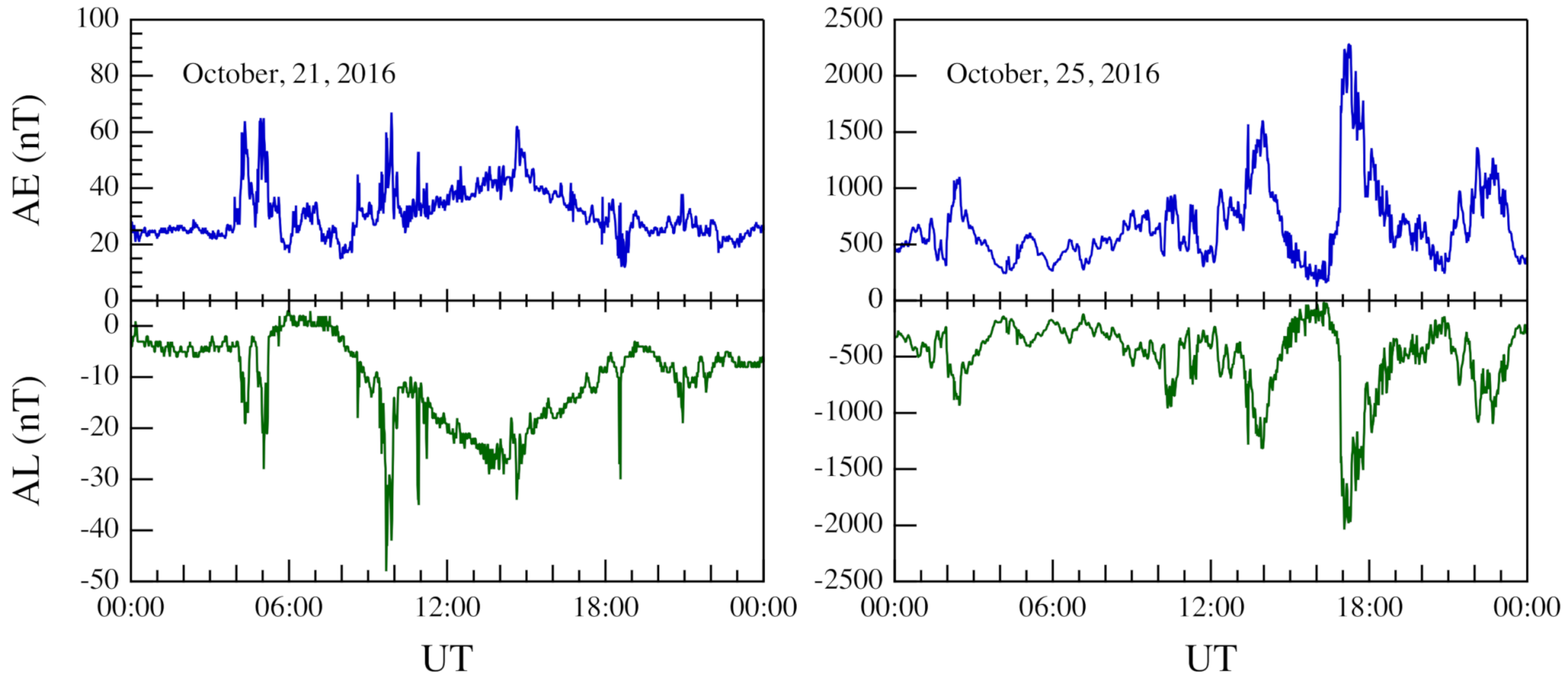
The average level of geomagnetic disturbance for the two days as estimated by the auroral electrojet AE index value was ∼30 nT and ∼660 nT, respectively. The daily behavior of the high-latitude geomagnetic disturbance level on the two selected days can be appreciated looking at Figure 1 where the AE and AL indices are plotted. We remind the reader that the AE and AL indices are proxies of the auroral electrojet currents flowing in the polar ionosphere [24]. In particular, the AE index provides an estimation of the energy deposition rate [26] and AL of the westward electrojet [27,28]. We note the quite different scales used in the plots relative to the first (left panel) and second (right panel) period.

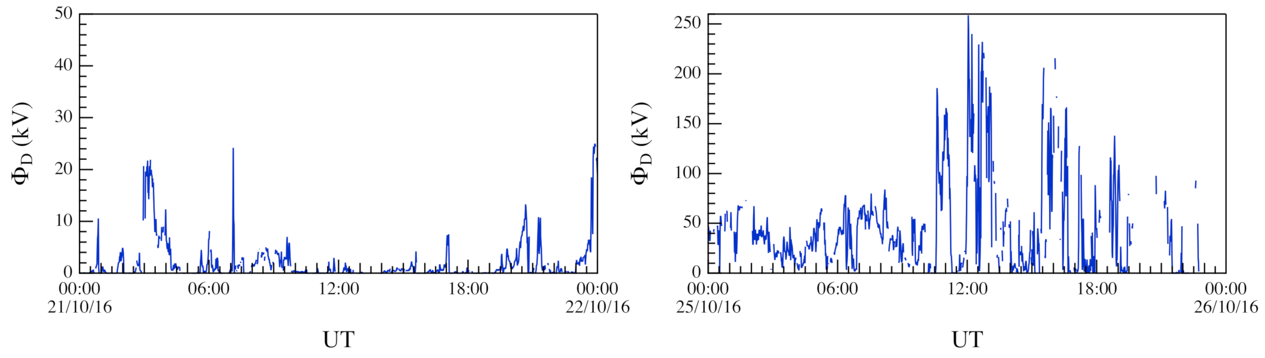
The two periods under study differed notably also for the amount of energy transmitted from the solar wind to the magnetosphere–ionosphere system. Following Milan et al. [29], we computed the dayside reconnection rate ${\Phi }_D$ for both days. Indeed, ${\Phi }_D$ plays the role of a coupling function between the solar wind and the Earth’s magnetosphere. According to Milan et al. [29], ${\Phi }_D$ is given by:

$${\Phi }_D=\Lambda v_x^{4/3}{B}_{yz}{sin}^{9/2}\frac{1}{2}\theta ,$$

(2)

where $\Lambda =3.3·{10}^5$ m${}^{2/3}$ s${}^{1/3}$ is a constant factor, $v_x$ is the x-component of the solar wind velocity, $B_{yz}=\sqrt{B_y^2+B_z^2}$ is the interplanetary magnetic field (IMF) intensity in the YZ-plane, and $\theta =arctan(B_y/B_z)$ is the tilt angle of the IMF in the YZ-plane. All the solar wind parameters’ components were in the GSM reference system and had a 1 min time resolution. Data came from OMNI dataset available at CDAweb (https://cdaweb.gsfc.nasa.gov/index.html/, accessed on 31 May 2021).

Figure 2 shows the obtained behavior of the ${\Phi }_D$ coupling function for the two selected days. The second day was characterized by a relevant increase of the energy transferred to the Earth’s magnetosphere. In particular, we found an average increase of the ${\Phi }_D$ coupling function by a factor >20 between 25 October and 21 October. Thus, substorm activity was practically absent during 21 October, while it was intense during 25 October. This was also confirmed by the inspection of the auroral emission (data not shown) as observed by the DMSP satellites (please refer to the Special Sensor Ultraviolet Spectrographic Imager (SSUSI) data, available at https://ssusi.jhuapl.edu/, accessed on 31 May 2021).

The second of these two intervals was already investigated in a previous work by Consolini et al. [19], where the multifractal structure of the local magnetic field fluctuations, as measured by Swarm satellites, was investigated. The new analysis performed here will permit studying the relation between the singularity features of FACs and the fractal/multifractal structure of the magnetic field fluctuations.

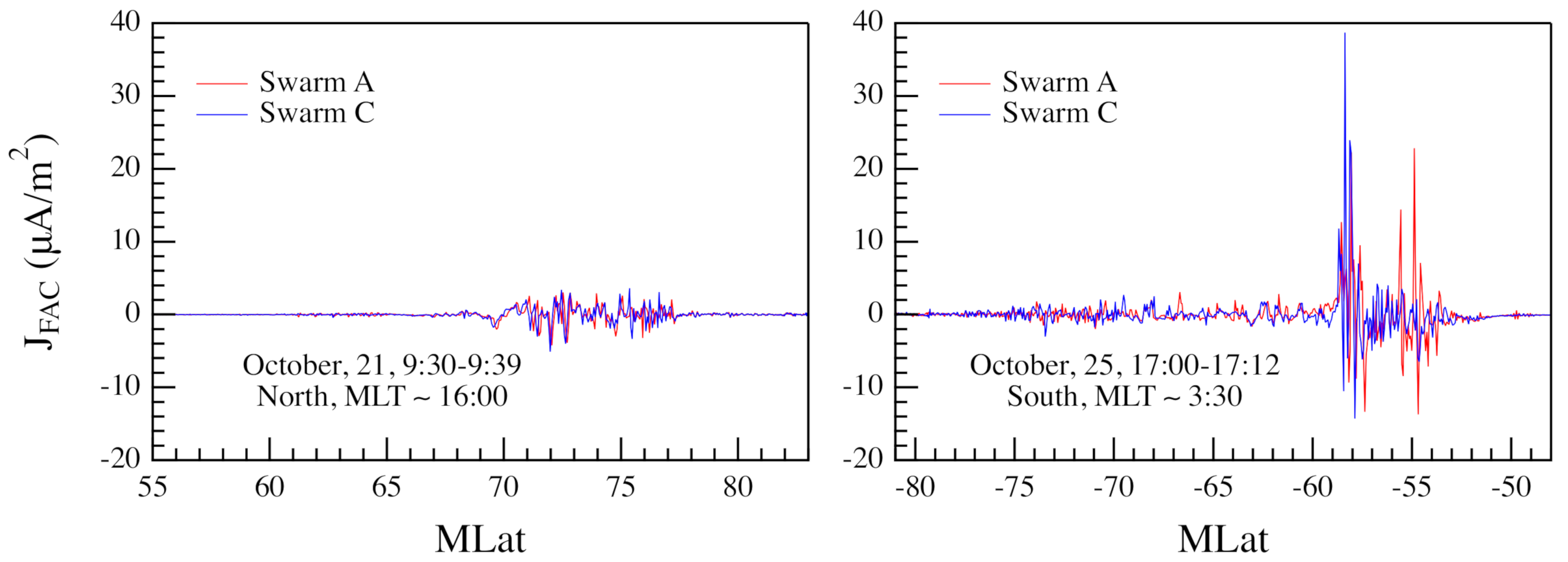
Figure 3 shows the FAC density, $J_{FAC}$, for two crossings of the Northern and Southern Hemispheres in correspondence with the lowest AL index periods of the two selected days. The variability of the FACs was higher on the day of maximum geomagnetic activity level, i.e., 25 October, than on the day with minimum activity, i.e., 21 October. Indeed, on 25 October, FACs’ intensity showed numerous positive and negative excursions, whose amplitude was much larger than on 21 October. This observation supported the hypothesis of the existence of a fine and filamentary structure of these currents.

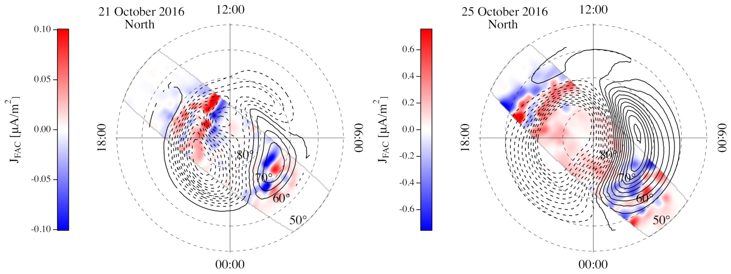
Figure 4 displays the average FAC patterns for the two selected days in the Northern Hemisphere in comparison with the electrostatic potential maps obtained by means of the CS10 statistical convection model by Cousins and Shepherd [30]. The CS10 model is a dynamical model based on the observations of the Super Dual Auroral Radar Network (SuperDARN) and provides the potential maps for any dipole tilt and IMF and solar wind conditions in a wide interval, independently for the Northern Hemisphere and the Southern Hemisphere. We noticed that during disturbed conditions (the right panel in Figure 4), the FACs intensified and flowed at lower latitudes, as expected. The FAC maps were computed using data from the Swarm A and C L2-FAC product and averaging over each day. The resolution used was $1^{\circ }\times 1^{\circ }$.

3. Methods: The Sign-Singularity Analysis

The properties of many physical processes can be described by fractal/multifractal probability measures (see, e.g., [31,32,33,34]). Generally, fractal/multifractal analysis deals with positive defined probability measures, which cannot capture some features of rapidly oscillating signals or quantities.

In contrast with positive measures, a signed measure can be useful to describe and characterize random fields that oscillate in sign. Indeed, a signed measure can take either positive or negative values and can show a different singular character, which may be used to characterize the complexity contained in rapidly oscillating quantities. The way to approach to signed measures was introduced by Ott et al. [23], who applied it to the investigation of kinematic dynamos and fluid turbulence. In particular, Ott et al. [23] applied the analysis of the sign-singular measure to the vorticity field in high-Reynolds fluid turbulence, which is characterized by oscillations in sign on a very fine scale. To quantify the sign-singular character of a signal $f(x)$, Ott et al. [23] introduced a scaling exponent $\kappa$, named the cancellation exponent, whose the q-th order generalization is analogous to the generalized dimension $D_q$ used in the case of the multifractal analysis [31]. Let us describe in detail the procedure introduced by Ott et al. [23].

Let X be a closed and finite interval, and let $f(x):X\to X$ be a zero-mean oscillating signal (i.e., ${\int }_{X}f(x)dx=0$). Consider a partition of size $ϵ$ covering the interval X, and define a signed-measure ${\mu }_{ϵ}({\Omega }_i)$ on each disjoint subset ${\Omega }_i(ϵ)\in X$ according to the following definition:

$${\mu }_{ϵ}({\Omega }_i)=\frac{{\int }_{{\Omega }_i(ϵ)}f(x)dx}{{\int }_X\mid f(x)\mid dx}.$$

(3)

The previous measure is said to be sign-singular if, given a subset ${\Omega }_i(ϵ)$ in which ${\mu }_{ϵ}({\Omega }_i)\ne 0$, there is a sub-subset ${\Omega }_j({ϵ}^{\prime })\in {\Omega }_i(ϵ)$ in which $\left[{\mu }_{ϵ}({\Omega }_i)\right]=-\left[{\mu }_{{ϵ}^{\prime }}({\Omega }_j)\right]$, i.e., the measure changes its sign on an arbitrary fine scale $ϵ$.

Using the coarse-grained signed measure ${\mu }_{ϵ}({\Omega }_i)$, it is possible to introduce an associated partition function $\chi (ϵ)$,

$$\chi (ϵ)=\sum _i\mid {\mu }_{ϵ}({\Omega }_i)\mid ,$$

(4)

where the sum runs over all the i-th subsets. The sign-singular character of the signed measure can then be evaluated by computing the so-called cancellation exponent, $\kappa$, defined as:

$$\kappa =-\underset{ϵ\to 0}{lim\; sup}\frac{ln\chi (ϵ)}{lnϵ}.$$

(5)

According to the previous definition, we clearly have that for a positive and normalized measure, such as a probability measure, we have $|{\mu }_{ϵ}({\Omega }_i)|\equiv {\mu }_{ϵ}({\Omega }_i)\to {\sum }_i{\mu }_{ϵ}({\Omega }_i)=1$, so that $\kappa =0$. Conversely, for a non-positive sign-singular measure, $\kappa >0$, at least on scales larger than a cut-off below which the measure is regular and smooth with a well-defined sign.

In the case of one-dimensional (1D) signals, the cancellation exponent $\kappa$ generally ranges in the interval $\kappa \in [0,1]$. In particular, it has been shown that for Brownian motions and Markovian stochastic signals, the cancellation exponent is $\kappa =1/2$, while for non-differentiable signals, $\kappa =1$ [35,36]. More generally, if d is the signal dimension, then for a stochastic signal, $\kappa =d/2$ [36].

As shown in different studies of either fluid and magnetohydrodynamic (MHD) turbulence [35,36,37,38], the value of the cancellation exponent can be linked to other scaling features and, in particular, to the scaling exponent $\gamma (1)$ of the first-order structure function. Indeed, in the case of the Kolmogorov scaling, the first-order structure function of the fluid velocity at the scale $ϵ$ is related to the partition function $\chi (ϵ)$ by the relation,

$$\langle |v_{\Vert }(\overrightarrow{r}+\overrightarrow{ϵ})-v_{\Vert }(\overrightarrow{r})|\rangle \simeq ϵ\chi (ϵ),$$

(6)

such that:

$$\kappa =1-\gamma (1).$$

(7)

Vainshtein et al. [37] showed that in the case of the Kolmogorov K41 theory for fully developed turbulence, the cancellation exponent $\kappa$ corresponds to the vorticity scaling index, $\kappa =2/3$.

Furthermore, in the case of turbulent flows, as shown by Sorriso-Valvo et al. [39], the cancellation exponent $\kappa$ can be linked to the fractal dimension D of the structures by the relation,

$$\kappa =\frac{1}{2}(d-D).$$

(8)

Here, d is the system dimension. According to this equation, the cancellation exponent provides information on the co-dimension of the flow structures in turbulent fields [39].

The sign-singularity analysis has been applied in several different fields from fluid turbulence (see, e.g., [23,37]) to magnetohydrodynamic turbulence (see, e.g., [39,40,41]), the photospheric magnetic field in flaring regions (see, e.g., [42,43]), etc.

In this work, we applied the sign-singularity analysis to the FACs as estimated by the ESA-Swarm magnetic field measurements [25]. In detail, we introduced the following signed measure,

$${\mu }_{\tau }({\Omega }_i)=\frac{{\sum }_{t_k\in {\Omega }_i(\tau )}{J}_{FAC}(t_k)}{{\sum }_{t_k\in T}\mid J_{FAC}(t_k)\mid },$$

(9)

where $J_{FAC}(t_k)$ is the FAC density measured at time $t-k$, ${\Omega }_i(\tau )\in T$ is an element of the partition of the time interval T, and $\tau$ is the dimension (scale) of the partition element. Then, we computed the associated partition function $\chi (\tau )$,

$$\chi (\tau )=\sum _i\left|{\mu }_{\tau }({\Omega }_i)\right|,$$

(10)

which according to Equation (5) is expected to scale at short $\tau$ as:

$$\chi (\tau )\propto {\tau }^{-\kappa }$$

(11)

in the case of a sign-singular measure. However, more in general, we searched for scaling intervals where the partition function followed the behavior reported in Equation (11). This was because when dealing with real signals, the scaling features can be observed in a limited range of scales.

4. Results and Discussion

The sign-singularity analysis of FACs was performed by analyzing separately the Northern and Southern Hemisphere crossings to investigate if there was any significant difference on the scaling features in the two hemispheres. This was justified by the fact that there is much evidence for a north–south asymmetry in the processes taking place in the polar ionospheric region, which could be a consequence of the different topology of the geomagnetic field and the different insolation/seasonal conditions [44,45,46,47].

We analyzed the scaling of the signed measure over a selected set of temporal scales in the range between 1 s and ∼150 s for each crossing (we remind that we had to construct a partition of the time interval, so that the set of temporal scales corresponded to the divisors of the total number of points available), and then, the obtained partition functions were averaged for each hemisphere and high-latitude geomagnetic disturbance level. Assuming that there was a simple linear relationship between the temporal scale $\tau$ and the corresponding spatial scale ℓ, i.e., $\ell \sim v_s\tau$ where $v_s\simeq 8$ km/s is the satellite speed, then the investigated range of temporal scales corresponded to an interval of spatial scales given by $\ell \in [8,1200]$ km. The link between temporal and spatial scales was valid assuming that the satellite speed was sufficiently large to ensure that the crossing time of the current structures was faster than their typical evolution time [22]. Clearly, this was a first-order approximation, because we should also have to consider the fast dynamics of these current systems in relating temporal and spatial scales.

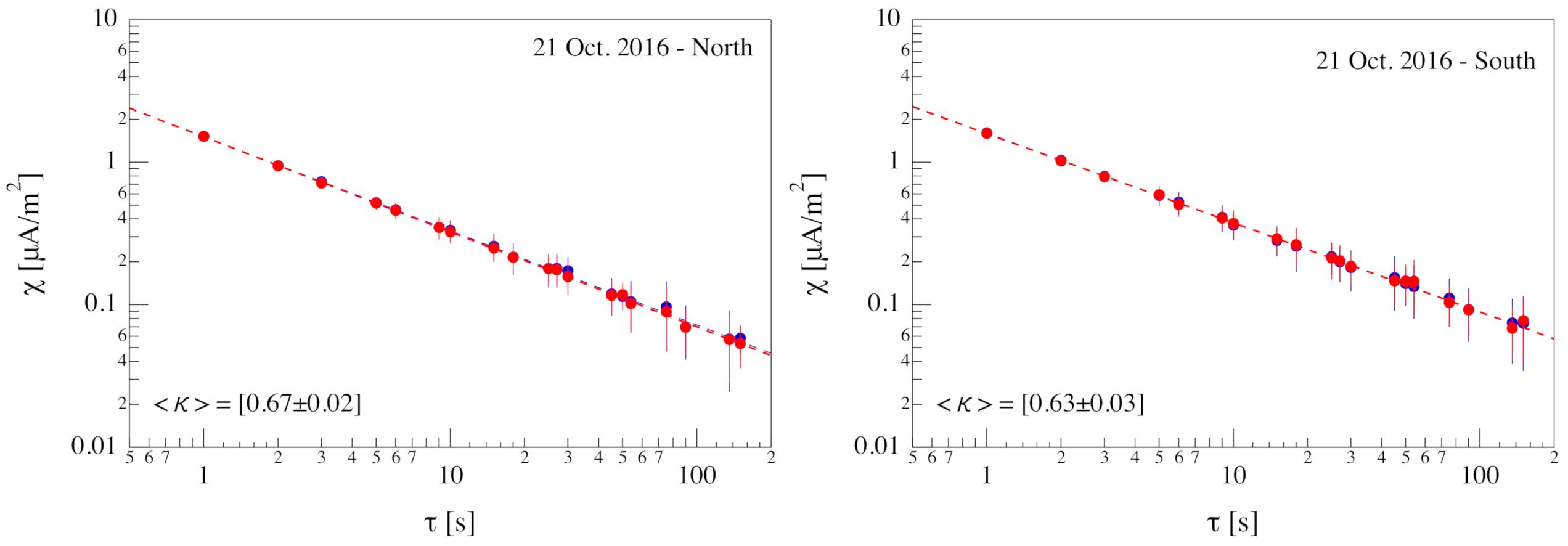
We started our analysis by investigating the sign-singularity feature of the FACs for the first of the two selected days, i.e., 21 October. Figure 5 shows the behavior of the partition function $\chi (\tau )$ averaged on the Northern (left) and Southern (right) Hemisphere crossings of the polar ionosphere by the two considered Swarm satellites (Swarm A and C). In our analysis, we did not consider dayside and nightside FAC crossings separately, because from a preliminary check, we did not find any substantial difference in the scaling features (not shown), which were the core of our analysis. This was reasonable to assume since, if the physical mechanisms acting at the investigated timescales were the same, there would be no reason to expect different scaling features between the dayside and nightside FACs. The scaling of the partition function did not evidence any difference between the two satellites, supporting the quasi-stationary character of the FAC average structure. Furthermore, by fitting the scaling of the partition function $\chi (\tau )$ using a power-law, the cancellation exponent $\kappa$ for Northern and Southern Hemisphere crossings was very similar, being consistent inside the errors (data not shown). Thus, we can compute for the cancellation exponent the corresponding average values for the Northern and Southern Hemisphere crossings, which were $\langle \kappa \rangle =[0.67\pm 0.02]$ and $\langle \kappa \rangle =[0.63\pm 0.03]$, respectively.

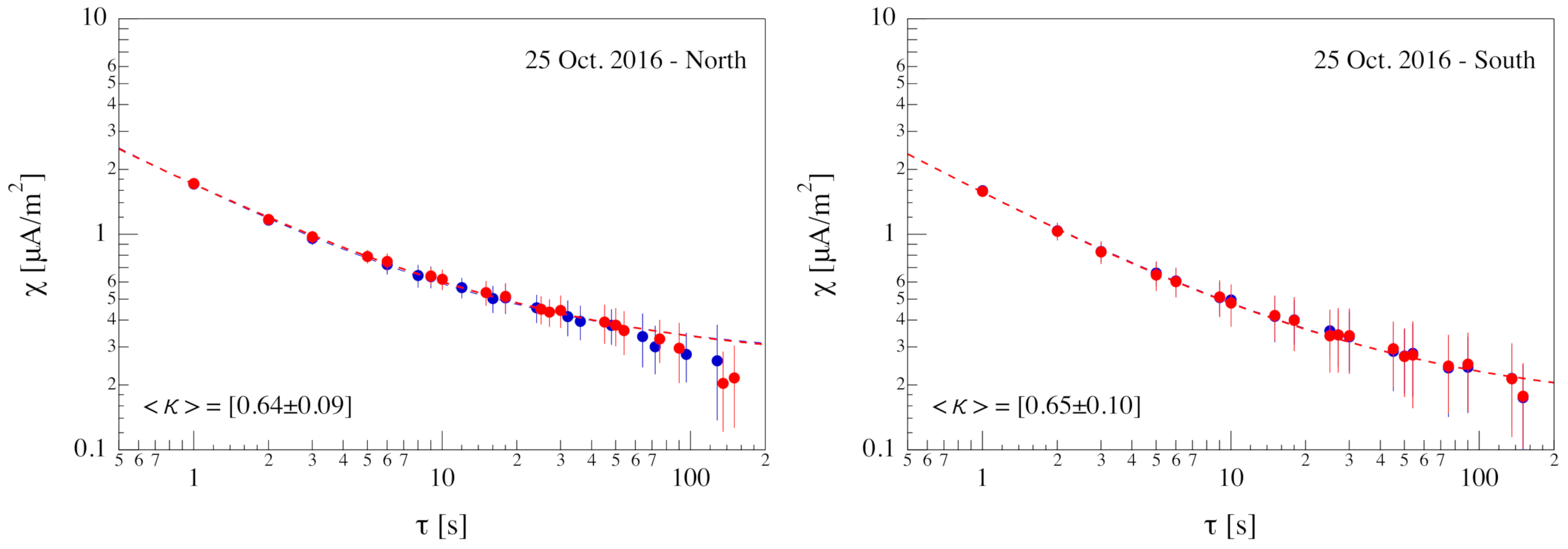
Figure 6 shows the partition function $\chi (\tau )$ averaged on the Northern (left) and Southern (right) Hemisphere crossings of the polar ionosphere for 25 October. Different from the previous case, the power-law scaling of the partition function $\chi (\tau )$ seemed to be essentially confined to the shortest timescales, i.e., $\tau <$ 10–20 s. Furthermore, at timescales $\tau$ larger than 20 s, the partition function tended to flatten. This different character could be due to the persistence of a specific sign for the FACs at large spatial scales during disturbed conditions. We will return to this point in the next section.

In order to obtain a reliable estimation of the cancellation exponent in the limit of $\tau \to 0$ for this last case, we fit the partition function $\chi (\tau )$ using a power-law plus a constant value, which accounted for the flattening at long $\tau$ values, i.e.,

$$\chi (\tau )=a_0{\tau }^{-\kappa }+a_1.$$

(12)

As a result, we obtained for the cancellation exponent, in the limit of short $\tau$, i.e., in the limit of $\tau \to 0$, an average value $\langle \kappa \rangle =[0.64\pm 0.09]$ and $\langle \kappa \rangle =[0.65\pm 0.10]$ for the Northern and Southern Hemisphere crossings, respectively. Again, the obtained values of the cancellation exponent were very similar. However, although here, we used the expression of Equation (12) to estimate the short timescale scaling exponent, the behavior observed at longer timescales ($\tau >10$ s) could be due to the emergence of a different scaling regime. This point is investigated below.

Since the values of $\kappa$ obtained under different geomagnetic (substorm activity) conditions and in both hemispheres were consistent each other in the limit of short $\tau$, we computed a mean value of the cancellation exponent, $\kappa$, which resulted in:

$${\kappa }^{\prime }=[0.65\pm 0.06].$$

(13)

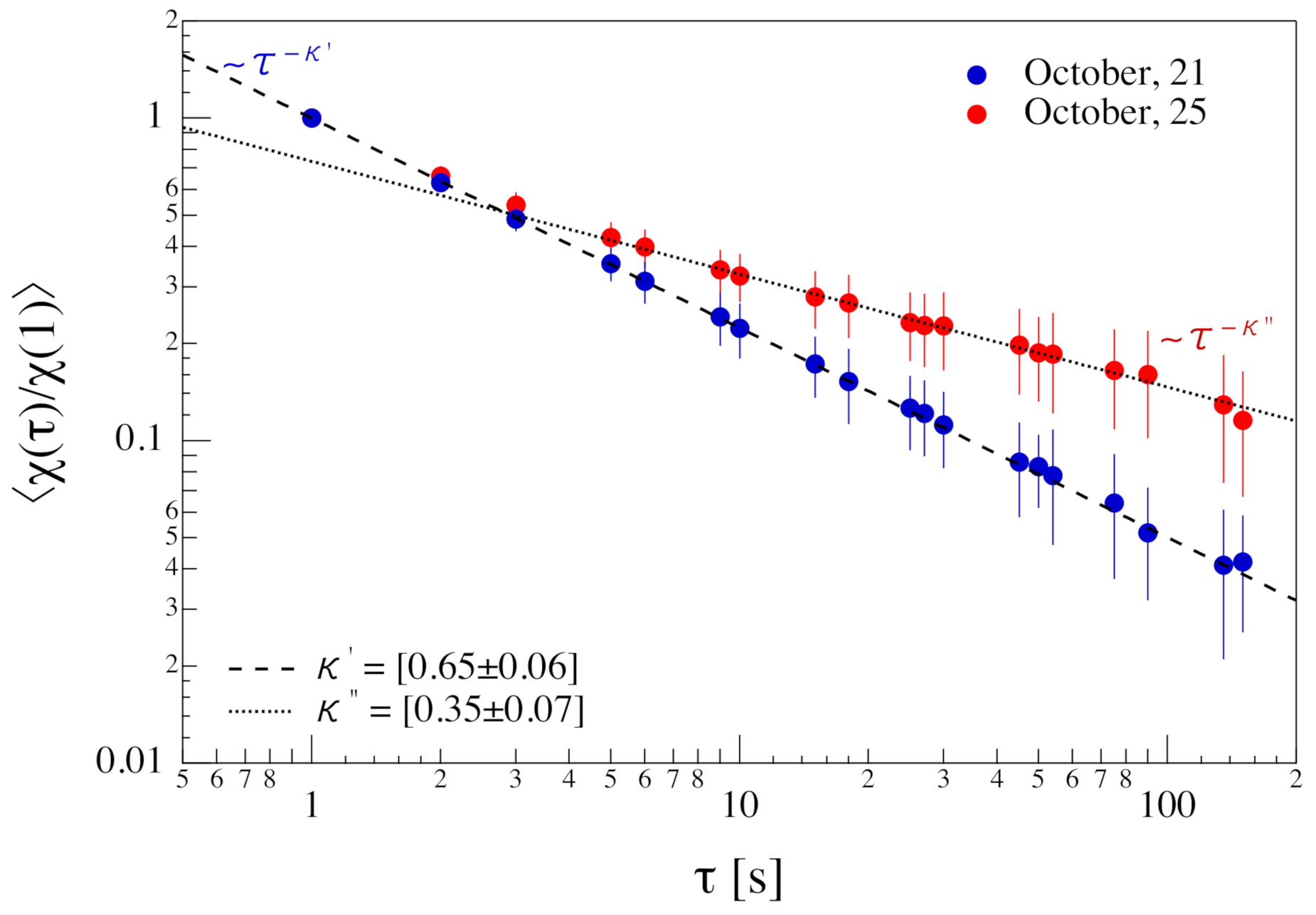
Furthermore, the similar behavior of the dependence on $\tau$ of the partition functions $\chi (\tau )$ relative to the Northern and Southern Hemisphere crossings reported in Figure 5 and Figure 6 suggested that for each of the two considered days, we could average the partition functions between the two hemispheres, so obtaining the average trends of the partition function for the two different geomagnetic conditions. The results are plotted in Figure 7, which shows the different behavior of the mean normalized partition function, $\langle \chi (\tau )/\chi (1)\rangle$, under the different high-latitude geomagnetic disturbance level. The mean was computed by firstly normalizing each partition function to the value for $\tau =1$ s ($\chi (1)$) and successively averaging the re-scaled partition functions.

From the average behavior of the partition functions reported in Figure 7, we can see how the scaling, in the limit of small $\tau$ ($\tau <4$ s), tended to be the same. This result suggested that the cancellation properties of FACs were the same for small scales and that the sign-singularity was a genuine property of the fine structure of FACs. Furthermore, the departure from the power-law scaling of the average partition function relative to 25 October for $\tau >4$ s suggested that during substorm periods, there could be the formation of a more homogeneous and persistent structure of FACs at spatial scales larger than ∼30 km. We note that the value of $\tau \sim 4$ s actually represented a sort of limit between two different domains of the cancellation exponent. Indeed, by averaging the partition functions for the disturbed case (25 October), a new scaling domain emerged for $\tau >4$ s, which was characterized by a cancellation exponent ${\kappa }^{″}=[0.35\pm 0.07]$. The smaller value of the cancellation exponent, ${\kappa }^{″}$, observed in this domain was the signature of a less inhomogeneous and more persistent character of the FACs during disturbed geomagnetic conditions. The existence of two scaling regimes for the partition function was confirmed by a Levenberg–Marquardt nonlinear weighted fitting procedure using two merged power-laws, which returned a ${\chi }^2$ value reduced by a factor of 20 in comparison to a single power-law fit.

Although the value of the cancellation exponent in the limit of small scales, i.e., ${\kappa }^{\prime }=[0.65\pm 0.06]$, agreed with the expected value for fluid turbulence [37], we believe that a more appropriate framework to discuss the observed value would be that of Hall MHD turbulence in the presence of a strong guiding magnetic field [41]. Indeed, assuming that the magnetic field in the region of the FACs can be written as $\mathbf{B}(x,y)=[\delta B_1(x,y),\delta B_2(x,y),B_0(x,y)]$ with $\delta B_{1,2}\ll B_0$ the horizontal components and $B_0$ the vertical component, the current field along the main magnetic field component $B_0$ would be $J_0(x,y)={(\nabla \times \mathbf{B})}_0=({\partial }_1\delta B_2-{\partial }_2\delta B_1)$; in other words, the vertical current (in our case, the FAC) was related to the helicity of the horizontal magnetic field. Our value of $\kappa$ in the limit of small scales Hemisphere quite well with the transverse cancellation exponent of the current ($j_z$) parallel to the strong guide field observed by Martin et al. [41] in the MHD domain, the transverse cancellation exponent for the current $j_z$ being ${\kappa }_{\perp }^z\sim 0.75$. Furthermore, according to Sorriso-Valvo et al. [39], using Equation (8), it was possible to evaluate the fractal dimension $D_{\perp }$ of the current structures, which was $D_{\perp }=[1.7\pm 0.1]$, having posed for the system dimension $d=3$. Again, this value was not far from the $D_{\perp }^{j_z}=1.5$ found by Martin et al. [41].

The scaling break observed in the case of disturbed periods can be read as a symmetry-breaking. The term symmetry-breakingwas, here, used to indicate that the previous situation of an extended scaling symmetry over more than two decades was now broken at timescales larger than 4 s with the emergence of a new scaling regime, characterized by a different cancellation exponent. Indeed, the sign-singularity features of FACs in this situation showed a different character above or below the break timescale $\tau =4$ s (or spatial scale $\ell \simeq 30$ km). The emergence of such a symmetry-breaking in the partition function could be the counterpart of a dynamical topological phase transition of FACs that follows the increase of the geomagnetic activity level due to the occurrence of a substorm and that could be responsible for the generation of large current structures, perhaps related to the substorm current wedge. In other words, the FACs structure underwent a topological transition as a function of the substorm activity. Fitting the behavior of the average partition function by a power-law in the range $\tau \in [5,100]$ s, a different value for the cancellation exponent $\kappa$ was found, being in the range ${\kappa }^{″}=[0.35\pm 0.05]$. The corresponding fractal dimension $D_{\perp }$ of the current structures was $D_{\perp }=[2.3\pm 0.1]$. This value was not far from $D=2$, suggesting that the increased geomagnetic activity during magnetic substorms, which was associated with an enhancement of the FACs also due to the substorm current wedge, tended to generate more uniform current structures in this range of scales.

The above findings can be also explained in the framework of MHD equilibria. Indeed, since FACs flow along the main magnetic field in the MHD approximation, they need to satisfy the condition $\mathbf{j}=\alpha (\mathbf{r})\mathbf{B}$, together with the Gauss law $\nabla ·\mathbf{B}=0$. Assuming $\mathbf{B}={\mathbf{B}}_{\Vert }+{\mathbf{B}}_{\perp }$, we have ${\mathbf{j}}_{\Vert }=\alpha (\mathbf{r}){\mathbf{B}}_{\Vert }$, where $\alpha (\mathbf{r})$ is a measure of the spatial inhomogeneity of the field fluctuations that must be constant along field lines [1]. If the system is homogeneous $\alpha (\mathbf{r})\sim \alpha$ and the solutions of the so-called Beltrami fields’ equation $\mathbf{j}=\nabla \times \mathbf{B}=\alpha \mathbf{B}$ can only be cast in the form of a strong guided magnetic field configuration, i.e., $\mathbf{B}=[\delta B_1,\delta B_2,B_0(x,y)]$ with $\delta B_{1,2}\ll B_0$, this corresponds to the case of the increased geomagnetic activity during magnetic substorms, where more uniform field-aligned current structures are observed. Conversely, if the system is inhomogeneous, its solutions can be found in the form $\nabla \times {\mathbf{B}}_{\perp }\propto {\mathbf{B}}_{\Vert }$ with $\nabla ·{\mathbf{B}}_{\perp }=-\nabla ·{\mathbf{B}}_{\Vert }$, thus reducing the effective degrees of freedom of the system (${\mathbf{B}}_{\perp }$ and ${\mathbf{B}}_{\Vert }$ be coupled to each other), corresponding to the case of a lower fractal dimension $D_{\perp }$.

5. Summary and Conclusions

The results of our sign-singularity analysis of the FACs structure for different geomagnetic disturbance levels can be summarized as follows:

(i)

sign-singularity is a common feature of FACs;

(ii)

during periods of quiet geomagnetic conditions, the sign-singularity character of FACs is the same over at least two orders of magnitude ($\tau \in [1,100]$ s), and it is characterized by a cancellation exponent ${\kappa }^{\prime }\sim 0.63$;

(iii)

during periods of disturbed geomagnetic conditions, i.e., substorm times, we observed the occurrence of a symmetry-breaking in the sign-singularity features of the FACs, which were characterized by the same cancellation exponent of quiet conditions at the shortest timescales ($\tau <4$ s), but not at long timescales ($\tau >4$ s), where the cancellation was ${\kappa }^{″}\sim 0.33$.

These results suggested that the FACs undergo a topological change during geomagnetic substorms, which is characterized by an increase of the fractal dimension $D_{\perp }$. In particular, during geomagnetic substorms, the filamentary character of the FACs tends to be less marked, the current structure being more similar to sheets. However, this behavior generally occurs in a limited range of spatial scales, i.e., for $\ell \in [40,800]$ km. Conversely, going to smaller scales, a more filamentary character of the FACs still persists also during geomagnetic substorms. The emerging scenario is that of filamentary current structures that during substorm times may be embedded in larger current structures, more similar to sheets. We remark that this view of a filamentary structure of FACs at scales below 40 km is quite well in agreement with the multifractal character of the magnetic field fluctuations in the direction perpendicular to the main geomagnetic field at scales shorter than 80 km [19]. The emerging scenario is thus the one proposed by Wu and Chang [21], Wu and Chang [22] and also described in Consolini et al. [19], which claimed for the occurrence of 2D reduced MHD intermittent turbulence.

Another relevant issue that emerged from the analysis was the independence of the sign-singular character of the FACs on the considered hemisphere. This is very interesting because in spite of the the well-known north–south asymmetry of several features in the high-latitude ionosphere, the scaling feature of FACs seems to be invariant. The north–south symmetry of the observed scaling features could be the signature that characterizes the sign-singularity character at the investigated temporal and spatial scales, which is essentially the same physical process. However, a clear dependence on the occurrence of substorms was found. This topological change of the FACs is believed to be due to FACs increasing as a consequence of the substorm current wedge.

In conclusion, we attempted a first study of the FAC morphology using the sign-singularity analysis. This preliminary study has to be considered as a proof of concept that requires further work in order to analyze the FACs at smaller scales, our investigation being limited to 1 s data. A further step could be to use high-resolution magnetic field measurements to obtain a more detailed description of FACs’ structure.