
Applications of Radar Data Assimilation with Hydrometeor Control Variables within the WRFDA on the Prediction of Landfalling Hurricane IKE (2008)

 and
and 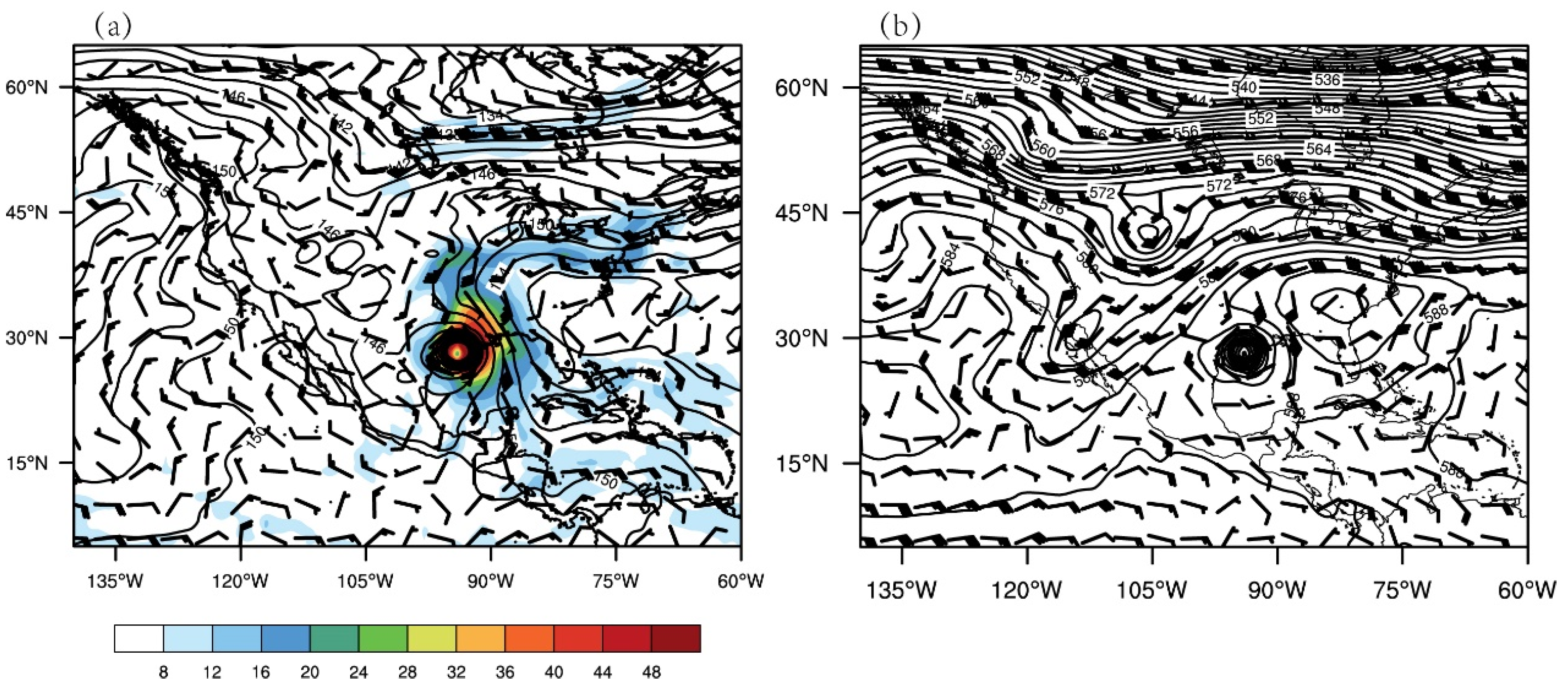
Abstract
:1. Introduction
2. Methodology
2.1. WRFDA 3DVar Data Assimilation System
2.2. Radar Observation Operator
3. Case Introduction and Experimental Setup
3.1. Hurricane IKE
3.2. Model and Experimental Design
4. Results
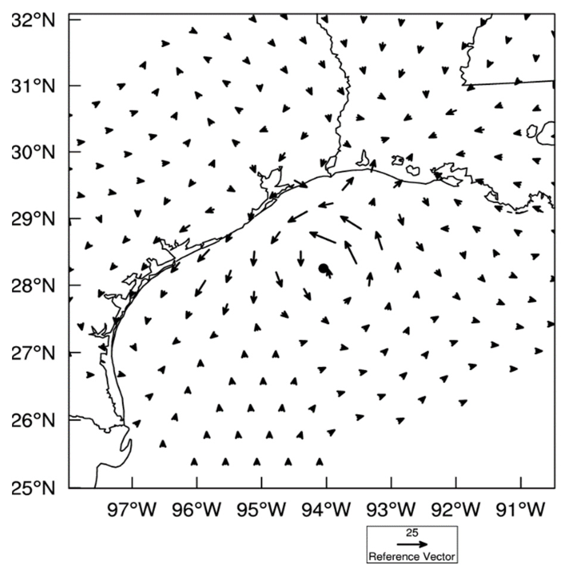
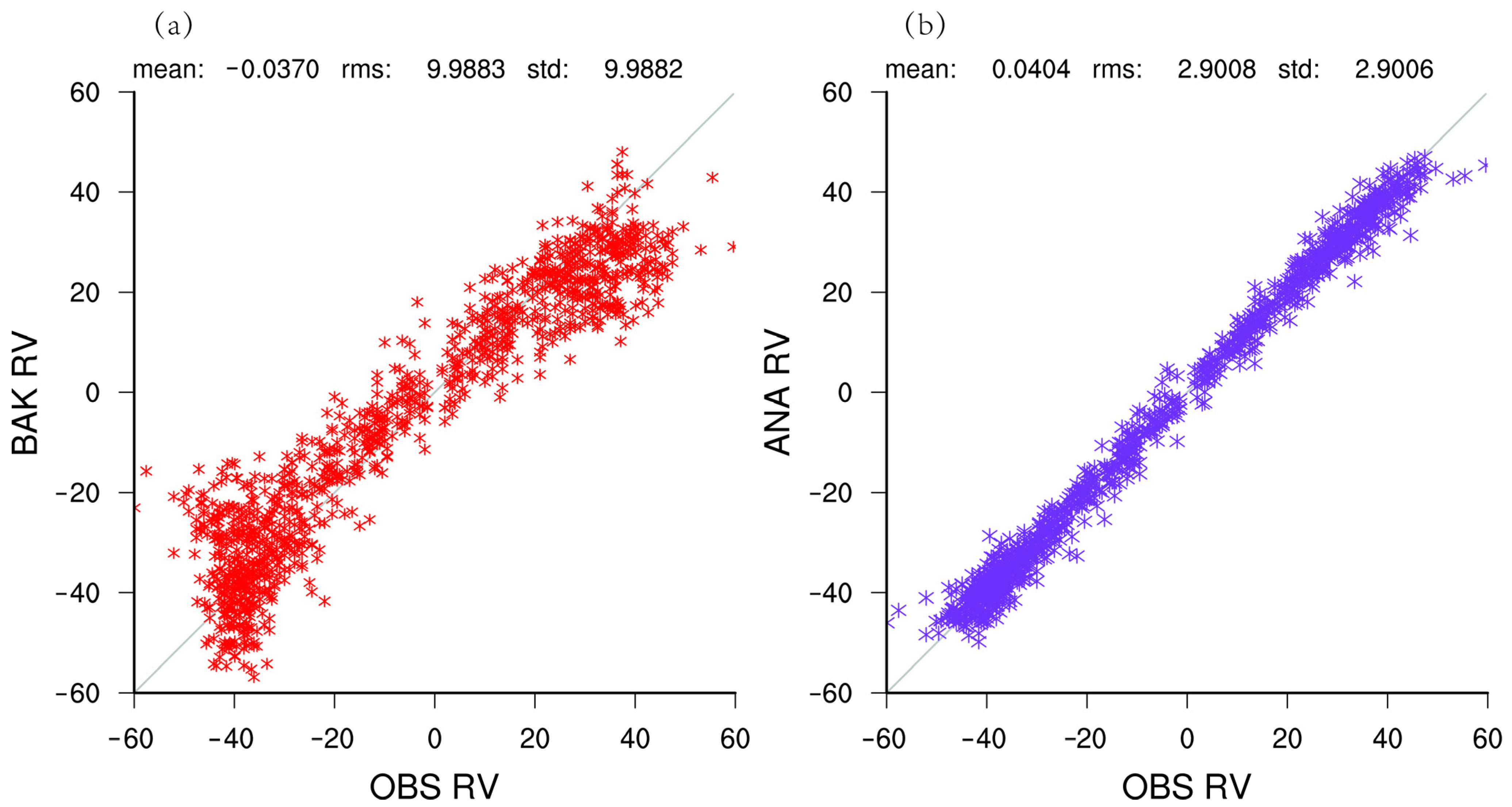
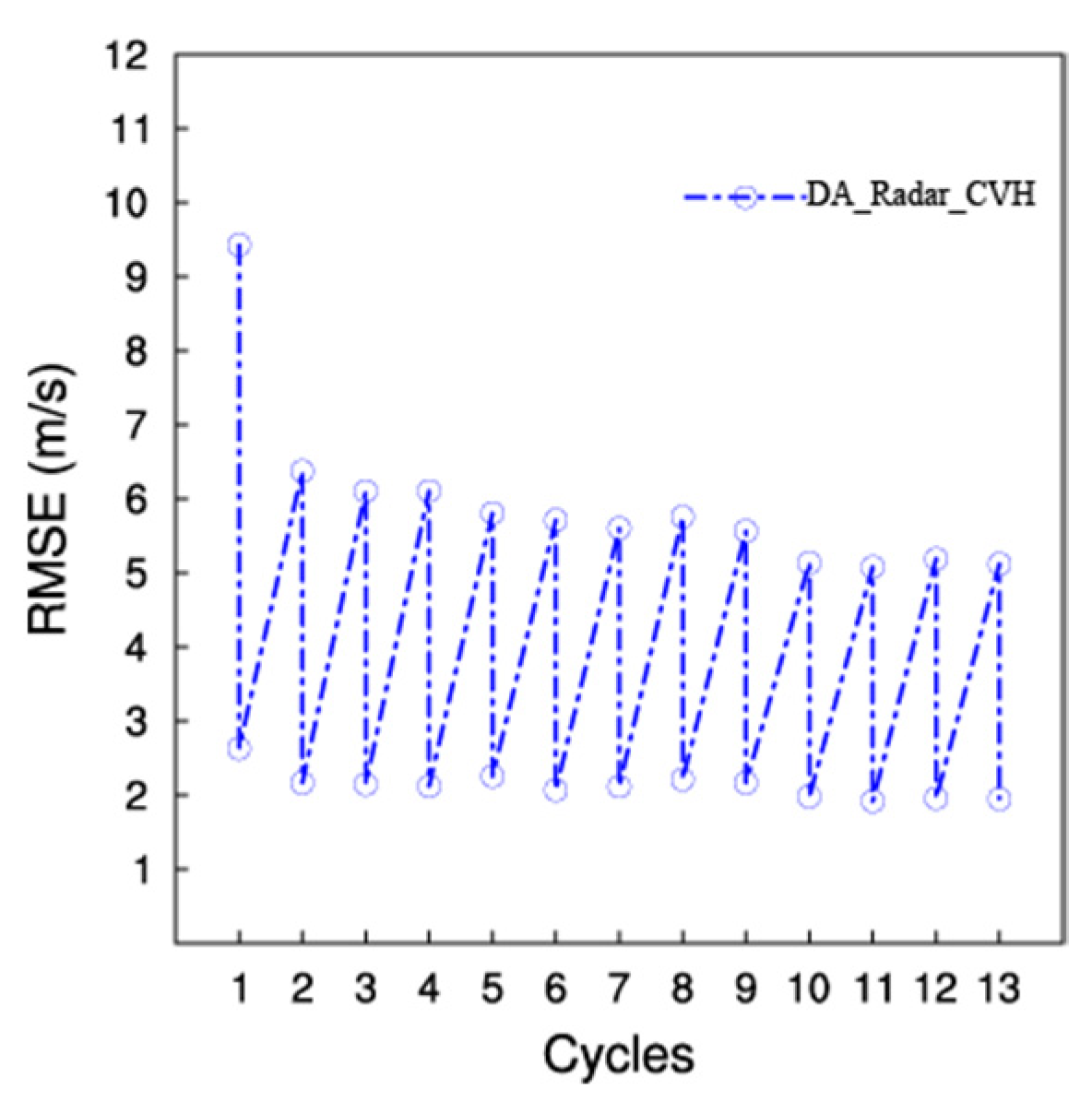
4.1. Wind Analysis
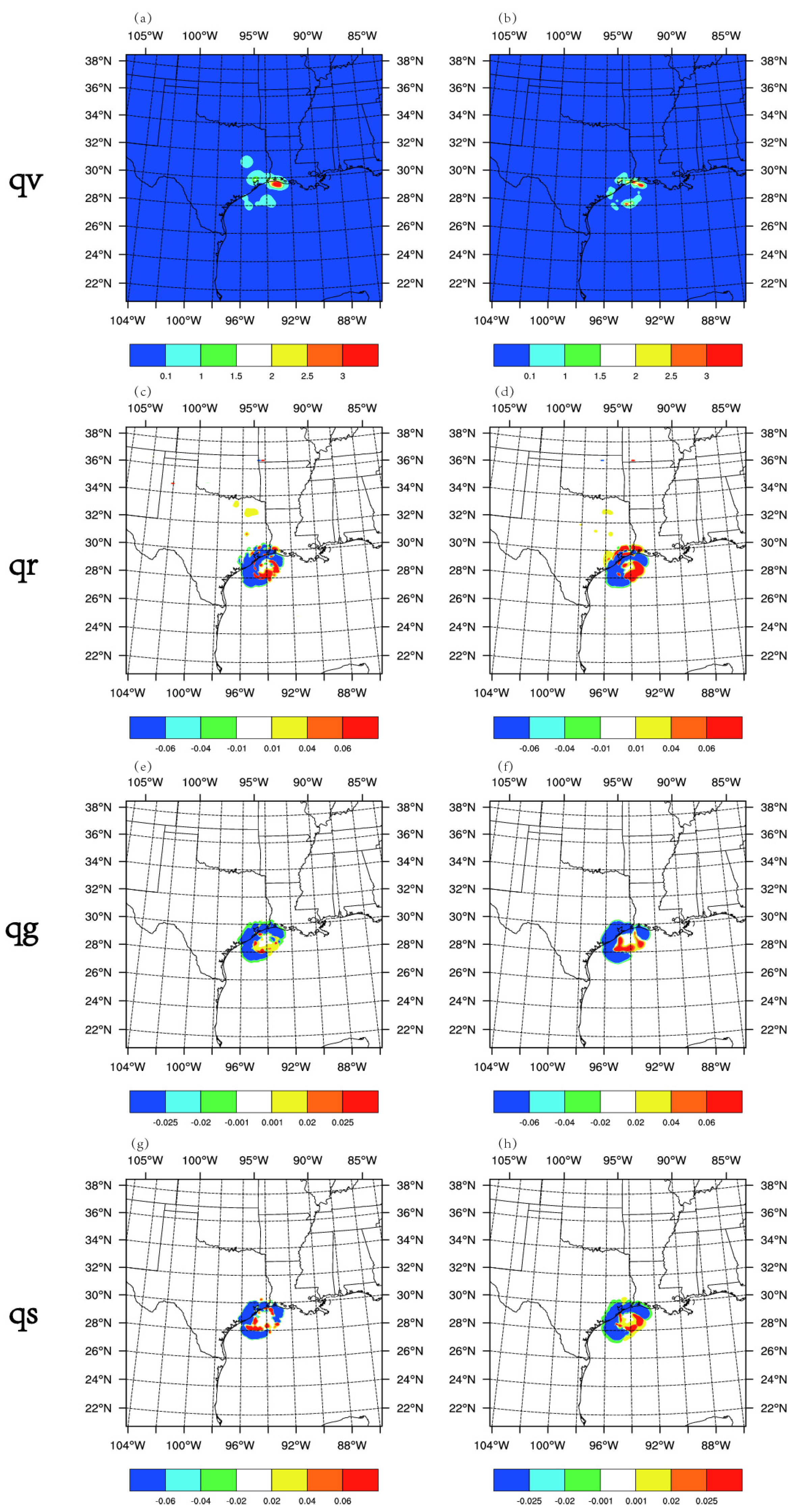
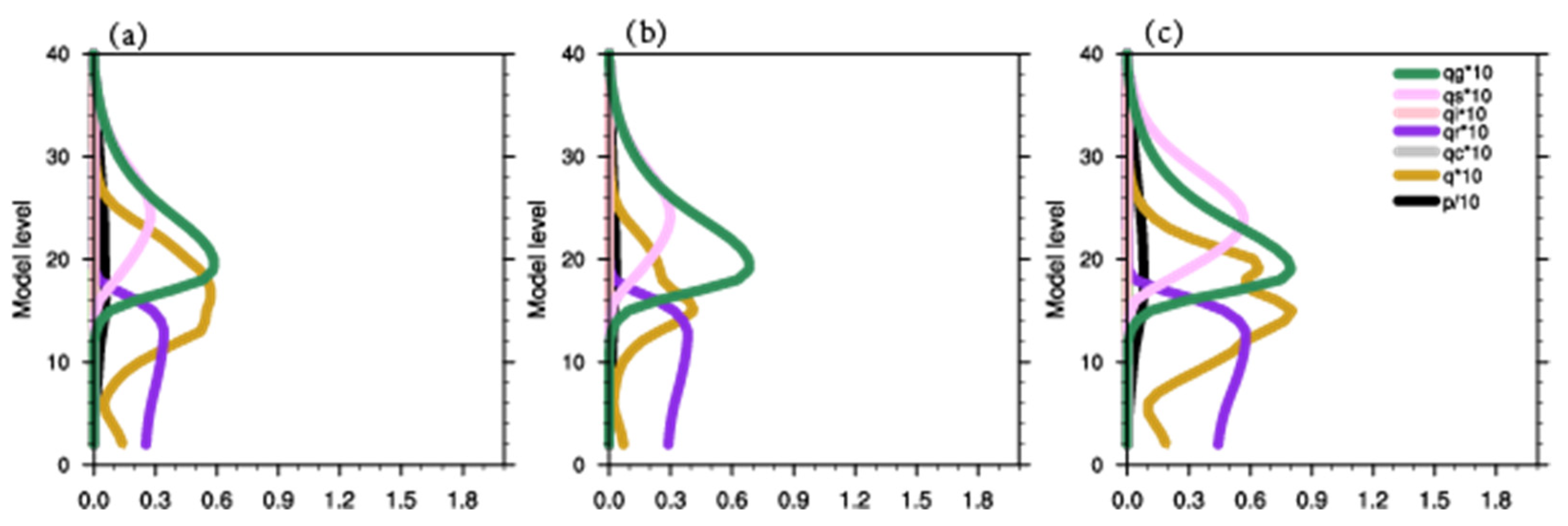
4.2. Increment for the Hydrometeors
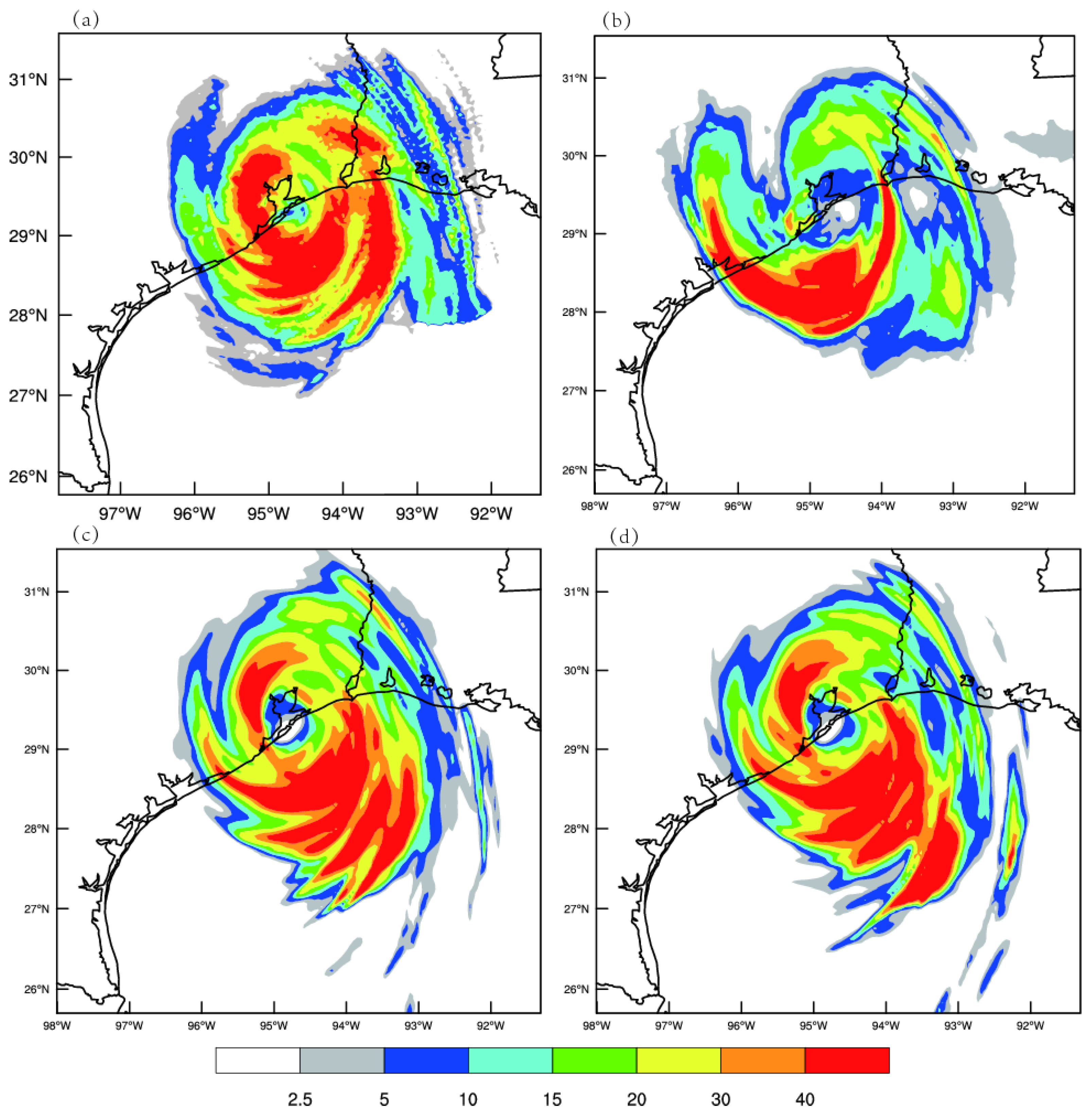
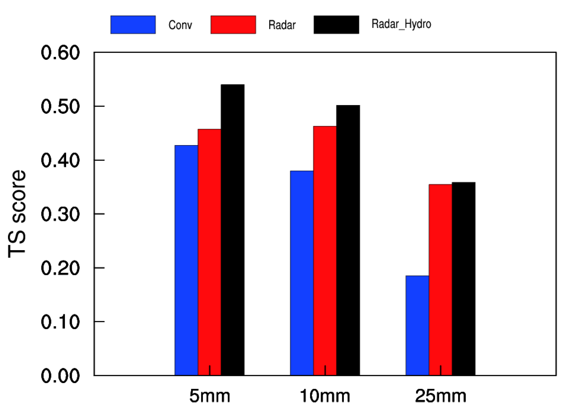
4.3. Precipitation Forecasts
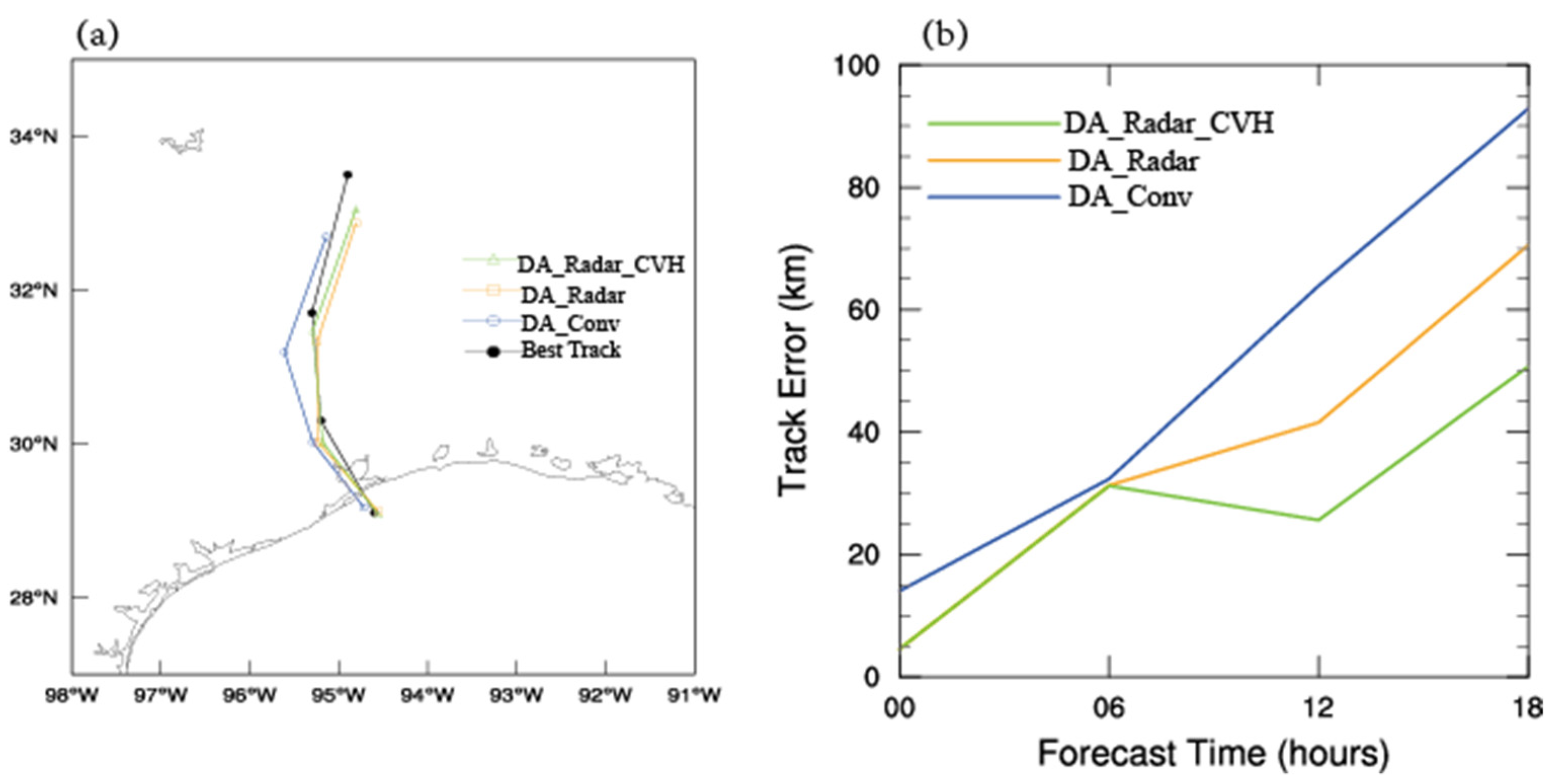
4.4. Track Forecasts
5. Summary
Author Contributions
Funding
Institutional Review Board Statement
Informed Consent Statement
Acknowledgments
Conflicts of Interest
References
- Dong, J.; Xue, M. Assimilation of radial velocity and reflectivity data from coastal WSR-88D radars using an ensemble Kalman filter for the analysis and forecast of landfalling hurricane Ike (2008). Q. J. R. Meteorol. Soc. 2013, 139, 467–487. [Google Scholar] [CrossRef] [Green Version]
- Sokol, Z. Assimilation of extrapolated radar reflectivity into a NWP model and its impact on a precipitation forecast at high resolution. Atmos. Res. 2011, 100, 201–212. [Google Scholar] [CrossRef]
- Courtier, P. The ECMWF implementation of three-dimensional variational assimilation (3D-Var). I: Formulation. Q. J. R. Meteorol. Soc. 1998, 124, 1783–1807. [Google Scholar] [CrossRef]
- Xiao, Q.; Kuo, Y.; Sun, J.; Xiao, Q.; Kuo, Y.H.; Sun, J.; Lee, W.C.; Barker, D.M.; Lim, E. An approach of radar reflectivity data assimilation and its assessment with the inland QPF of TC Rusa (2002) at landfall. J. Appl. Meteorol. Climatol. 2007, 46, 14–22. [Google Scholar] [CrossRef] [Green Version]
- Gao, J.; Stensrud, D. Assimilation of reflectivity data in a convective-scale, cycled 3DVAR framework with hydrometeor classification. J. Atmos. Sci. 2012, 69, 1054–1065. [Google Scholar] [CrossRef]
- Wang, H.; Sun, J.; Fan, S.; Huang, X.-Y. Indirect assimilation of radar reflectivity with WRF 3D-Var and its impact on prediction of four summertime convective events. J. Appl. Meteorol. Climatol. 2013, 52, 889–902. [Google Scholar] [CrossRef]
- Shen, F.; Xue, M.; Min, J. A comparison of limited-area 3DVAR and ETKF-En3DVAR data assimilation using radar observations at convective scale for the prediction of TC Saomai (2006). Meteorol. Appl. 2017, 24, 628–641. [Google Scholar] [CrossRef] [Green Version]
- Shen, F.; Xu, D.; Xue, M.; Min, J. A comparison between EDA-EnVar and ETKF-EnVar data assimilation techniques using radar observations at convective scales through a case study of Hurricane Ike (2008). Meteorol. Atmos. Phys. 2018, 130, 649–666. [Google Scholar] [CrossRef]
- Shen, F.; Xu, D.; Min, J. Effect of momentum control variables on assimilating radar observations for the analysis and forecast for TC Chanthu (2010). Atmos. Res. 2019, 230, 104622. [Google Scholar] [CrossRef]
- Shen, F.; Xu, D.; Min, J.; Chu, Z.; Xia, X. Assimilation of radar radial velocity data with the WRF hybrid 4DEnVar system for the prediction of hurricane Ike (2008). Atmos. Res. 2020, 234, 104771. [Google Scholar] [CrossRef]
- Xu, D.; Shen, F.; Min, J. Effect of background error tuning on assimilating radar radial velocity observations for the forecast of hurricane tracks and intensities. Meteorol. Appl. 2020, 27, e1280. [Google Scholar] [CrossRef] [Green Version]
- Derber, J.; Bouttier, F. A reformulation of the background error covariance in the ECMWF global data assimilation system. Tellus A 1999, 51, 195–221. [Google Scholar] [CrossRef]
- Sun, J.; Wang, H.; Tong, W. Comparison of the impacts of momentum control variables on high-resolution variational data assimilation and precipitation forecasting. Mon. Weather Rev. 2016, 144, 149–169. [Google Scholar] [CrossRef]
- Michel, Y.; Auligné, T.; Montmerle, T. Heterogeneous convective-scale background error covariances with the inclusion of hydrometeor variables. Mon. Wea. Rev. 2011, 139, 2994–3015. [Google Scholar] [CrossRef]
- Descombes, G.; Auligné, T.; Vandenberghe, F.; Barker, D.; Barre, J. Generalized background error covariance matrix model (GEN_BE v2.0). Geosci. Model Dev. 2015, 8, 669–696. [Google Scholar] [CrossRef] [Green Version]
- Meng, D.; Chen, Y.; Wang, H.; Gao, Y.; Potthast, R.; Wang, Y. The evaluation of EnVar method including hydrometeors analysis variables for assimilating cloud liquid/ice water path on prediction of rainfall events. Atmos. Res. 2019, 219, 1–12. [Google Scholar] [CrossRef]
- Zhao, Q.; Cook, J.; Xu, Q.; Harasti, P. Improving short-term storm predictions by assimilating both radar radial-wind and reflectivity observations. Weather Forecast. 2008, 23, 373–391. [Google Scholar] [CrossRef]
- Li, X.; Zeng, M.; Wang, Y.; Wang, W.; Wu, H.; Mei, H. Evaluation of two momentum control variable schemes and their impact on the variational assimilation of radar wind data: Case study of a squall line. Adv. Atmos. Sci. 2016, 33, 1143–1157. [Google Scholar] [CrossRef]
- Barker, D.; Huang, X.-Y.; Liu, Z.; Auligné, T.; Zhang, X.; Rugg, S.; Ajjaji, R.; Bourgeois, A.; Bray, J.; Chen, Y.; et al. The weather research and forecasting model’s community variational/ensemble data assimilation system: WRFDA. Bull. Am. Meteorol. Soc. 2012, 93, 831–843. [Google Scholar] [CrossRef] [Green Version]
- Ide, K.; Courtier, P.; Ghil, M.; Lorenc, A.C. Unified notation for data assimilation: Operational sequential and variational. Meteorol. Soc. 1997, 75, 181–189. [Google Scholar] [CrossRef] [Green Version]
- Wang, H.; Huang, X.; Sun, J.; Xu, D.; Zhang, M.; Fan, S.; Zhong, J. Inhomogeneous background error modeling for WRF-Var using the NMC method. Appl. Meteor. Clim. 2014, 53, 2287–2309. [Google Scholar] [CrossRef] [Green Version]
- Parrish, D.F.; Derber, J.C. The national meteorological center’s spectral statistical-interpolation analysis system. Mon. Weather Rev. 1992, 120, 1747–1763. [Google Scholar] [CrossRef]
- Xu, Q. On the choice of momentum control variables and covariance modeling for mesoscale data assimilation. J. Atmos. Sci. 2019, 76, 89–111. [Google Scholar] [CrossRef]
- Tong, M.; Xue, M. Ensemble Kalman filter assimilation of Doppler radar data with a compressible nonhydrostatic model: OSS experiments. Mon. Weather Rev. 2005, 133, 1789–1807. [Google Scholar] [CrossRef] [Green Version]
- Xu, Q.; Wei, L. Prognostic equation for radar radial velocity derived by considering atmospheric refraction and earth curvature. J. Atmos. Sci. 2013, 70, 3328–3338. [Google Scholar] [CrossRef]
- Sun, J.; Crook, N.A. Dynamical and microphysical retrieval from Doppler radar observations using a cloud model and its adjoint. Part I: Model development and simulated data experiments. Atmos. Sci. 1997, 54, 1642–1661. [Google Scholar] [CrossRef]
- Wang, H.; Sun, J.; Zhang, X.; Huang, X.-Y.; Auligné, T. Radar data assimilation with WRF 4D-Var. Part I: System development and preliminary testing. Mon. Weather Rev. 2013, 141, 2224–2244. [Google Scholar] [CrossRef]
- Xu, Q.; Wei, L.; Gu, W.; Gong, J.; Zhao, Q. A 3.5-dimensional variational method for Doppler radar data assimilation and its application to phased-array radar observations. Adv. Meteorol. 2010, 2010, 797265. [Google Scholar] [CrossRef] [Green Version]
- Wang, X. Application of the WRF Hybrid ETKF–3DVAR Data Assimilation System for Hurricane Track Forecasts. Weather Forecast. 2011, 26, 868–884. [Google Scholar] [CrossRef]
- Li, X.; Ming, J.; Xue, M.; Wang, Y.; Zhao, K. Implementation of a dynamic equation constraint based on the steady state momentum equations within the WRF hybrid ensemble-3DVar data assimilation system and test with radar T-TREC wind assimilation for tropical Cyclone Chanthu (2010). J. Geophys. Res. Atmos. 2015, 120, 4017–4039. [Google Scholar] [CrossRef] [Green Version]


Publisher’s Note: MDPI stays neutral with regard to jurisdictional claims in published maps and institutional affiliations. |
© 2021 by the authors. Licensee MDPI, Basel, Switzerland. This article is an open access article distributed under the terms and conditions of the Creative Commons Attribution (CC BY) license (https://creativecommons.org/licenses/by/4.0/).
Share and Cite
Shen, F.; Min, J.; Li, H.; Xu, D.; Shu, A.; Zhai, D.; Guo, Y.; Song, L. Applications of Radar Data Assimilation with Hydrometeor Control Variables within the WRFDA on the Prediction of Landfalling Hurricane IKE (2008). Atmosphere 2021, 12, 853. https://0-doi-org.brum.beds.ac.uk/10.3390/atmos12070853
Shen F, Min J, Li H, Xu D, Shu A, Zhai D, Guo Y, Song L. Applications of Radar Data Assimilation with Hydrometeor Control Variables within the WRFDA on the Prediction of Landfalling Hurricane IKE (2008). Atmosphere. 2021; 12(7):853. https://0-doi-org.brum.beds.ac.uk/10.3390/atmos12070853
Chicago/Turabian StyleShen, Feifei, Jinzhong Min, Hong Li, Dongmei Xu, Aiqing Shu, Danhua Zhai, Yakai Guo, and Lixin Song. 2021. "Applications of Radar Data Assimilation with Hydrometeor Control Variables within the WRFDA on the Prediction of Landfalling Hurricane IKE (2008)" Atmosphere 12, no. 7: 853. https://0-doi-org.brum.beds.ac.uk/10.3390/atmos12070853