Article

Application of Rough and Fuzzy Set Theory for Prediction of Stochastic Wind Speed Data Using Long Short-Term Memory

1
Department of Geomatics, National Cheng Kung University, Tainan 701, Taiwan
2
International College of Practice and Education for the Environment, International Program for Sustainable Development, Chang Jung Christian University, Tainan 71101, Taiwan
3
Department of Communications, Navigation and Control Engineering, National Taiwan Ocean University, Keelung 20224, Taiwan
4
Department of Soil and Water Conservation, National Chung Hsing University, 145 Xinda Road, Taichung 402, Taiwan
*
Author to whom correspondence should be addressed.
Submission received: 5 May 2021 / Revised: 9 July 2021 / Accepted: 14 July 2021 / Published: 17 July 2021
(This article belongs to the Special Issue Statistical Methods in Weather Forecasting)

Abstract

:
Despite the great significance of precisely forecasting the wind speed for development of the new and clean energy technology and stable grid operators, the stochasticity of wind speed makes the prediction a complex and challenging task. For improving the security and economic performance of power grids, accurate short-term wind power forecasting is crucial. In this paper, a deep learning model (Long Short-term Memory (LSTM)) has been proposed for wind speed prediction. Knowing that wind speed time series is nonlinear stochastic, the mutual information (MI) approach was used to find the best subset from the data by maximizing the joint MI between subset and target output. To enhance the accuracy and reduce input characteristics and data uncertainties, rough set and interval type-2 fuzzy set theory are combined in the proposed deep learning model. Wind speed data from an international airport station in the southern coast of Iran Bandar-Abbas City was used as the original input dataset for the optimized deep learning model. Based on the statistical results, the rough set LSTM (RST-LSTM) model showed better prediction accuracy than fuzzy and original LSTM, as well as traditional neural networks, with the lowest error for training and testing datasets in different time horizons. The suggested model can support the optimization of the control approach and the smooth procedure of power system. The results confirm the superior capabilities of deep learning techniques for wind speed forecasting, which could also inspire new applications in meteorology assessment.

1. Introduction

The depletion of fossil fuel resources, environmental pollution, and greenhouse effect have required the development of clean and safe energy sources for power generation [1,2]. Among different renewable energy alternatives, wind energy is considered as a promising and applied solution for making a renewable society and reducing emissions of greenhouse gas [3]. Wind is also abundant, inexhaustible, and affordable, which makes it a feasible, large-scale energy source alternative and one of the most sustainable ways of electricity generation. Despite being one of the fastest-developing energy sources in the world [1,4], due to the stochastic nature of wind speed, producing practical and sustainable energy becomes challenging for wind farms [3].
Since wind speed largely determines the amount of electricity generated by a turbine, accurate prediction can provide a reliable and secure source for the production of wind energy and also decrease the operating cost of the power system [3,5].
This also helps the power system to adapt the dispatch schedule in time according to changes in the input of wind power, ensures the quality of power, and reduces the cost of maintaining the service [6].
Since the time series of wind speed are mostly chaotic with stochastic characteristics, complex nonlinear approaches are needed for the forecasting tasks [7]. The wind speed prediction method can generally be divided into two groups: physical [8] and statistical approaches [9]. The physical models are plain methods, using physical data such as temperature, atmospheric pressure, obstacles and roughness [10]. While physical models may have satisfactory prediction potential, due to complicated meteorological conditions, difficult model initialization and extensive computation, their application is limited [11]. Statistical models have improved computational efficiency, but they also suffer from the weak generalization of learning the nonlinear characteristics, particularly for the wind speed series. The intelligent methods with the ability to map the nonlinear characteristics received great attention in the wind speed forecast field to address these disadvantages with its superior nonlinear fitting and generalization capabilities [5]. Potential applications for wind speed forecasting have been discussed in several studies in the literature. Chang et al. [12] suggested an improved neural network approach containing error feedback for forecasting short-term wind speed and power generation. In another piece of research, Noorollahi et al. [13] used ANN models to forecast temporal and spatial wind speeds in Iran.
In spite of numerous advantages of traditional neural networks [14], most of the architectures are shallow with weak generalization capability with less effective ability to learn complex patterns from highly erratic wind data [7]. Compared to the conventional neural network, deep learning algorithms with several layers of nonlinear functions can capture the characteristics of the wind speed time series more efficiently with lower parameters and computational costs [15,16].
The application of deep learning in time series modeling has drawn the attention of many researchers in recent years. For example, Lv et al. [17] proposed a deep learning method for traffic flow prediction with big data and Qiu et al. [18] suggested using an ensemble deep learning method to forecast electrical load. Additionally, deep learning methods have been successfully applied to the forecasting of wind speeds. Hu et al. [19] developed a deep auto-encoder-based model for short-term wind speed prediction using transfer learning. Wang [20] also developed a novel deterministic and probabilistic wind speed forecasting approach using deep belief network models.
A Recurrent Neural Network (RNN) is an extension of conventional deep learning neural networks incorporating connections that feedback the hidden layers of the neural network into themselves, called recurrent connections. However, due to the gradient disappearing, exploding problems, and trouble learning long-term patterns, RNNs are usually difficult to train [21].
Recently, the problem of gradient vanishing in RNNs was solved using the Long Short-Term Memory (LSTM) model [22]. Ma et al. [23] used LSTM to forecast traffic speed, showing that LSTM was capable of capturing the long-term temporal dependency of traffic data. In a study by Liu et al. [24], it is shown that an end-to-end deep learning architecture that combines convolution and LSTM is able to extract spatial-temporal traffic flow information. In the complex and deep processing of large, and long-term data series, LSTM has successfully achieved satisfactory functional application results [25,26].
For real-world applications, the management of uncertainty in datasets is important in any forecasting model, including LSTM. Rough and fuzzy sets, which provide valuable techniques that can be used to model data uncertainty as well as spatial relationships between data entities, are increasingly being used in different types of data sets [27]. Both theories model various forms of uncertainty.
In light of the value of energy alternatives and environmental pollution, the use of renewable energy has become a priority for people and governments throughout the Middle East, especially in Iran, where a variety of renewable energy sources are available and can be implemented to meet energy needs [28]. The wind turbine technology is quickly developing in the region concerning the efficient location, efficiency, and management scenarios. Based on a preliminary studies, regions located in the southern coasts of Iran are suitable for generating up to about 6500 megawatts electricity from the wind energy. The wind characteristics and assigned forecasts must, therefore, be studied in detail in order to provide an efficient wind resource assessment of Iran [29].
Therefore, this paper presents short-term wind speed forecasting using LSTM network with Rough Set Theory and Interval Type-2 Fuzzy Sets, with wind speed data obtained from international airport station located in southern coast of Iran, Bandar-Abbas City, the capital of the Hormozgan province. It is Iran’s largest port city and a vital economic and commercial hub. Bandar Abbas is also susceptible to tidal action, wave set-up, wind formation, and storm surges along the Persian Gulf and Oman Sea coasts [30]. Additionally, the Hormozgan Province is well-suited for wind turbine installation, as aerology data indicate that there are eight regions in this region with adequate wind energy capacity, one of which is Bandar Abbas City [31]. Wind forecasting data are, therefore, essential for a reliable and secure power generation system, especially at airports in developing countries. The lack of such knowledge may be the primary cause of the airport’s poor air traffic flow control and the delay of renewable energy projects. The Bandar Abbas International Airport is situated in a wide-open area with favorable wind patterns for air traffic. Wind activity is influenced by the surrounding topography, which blocks, intensifies, or changes the path of the wind as it passes, resulting in local wind effects that are not resolved by numerical weather prediction models. This airport’s characteristics make it ideal for researching the issue of wind speed downscaling as wind is heavily influenced by local topography and the nearby sea at the study site. Importantly, the lack of knowledge and related studies about wind speed at international airports is a major impediment to the airport’s sustainable development and accurate short-term wind speed forecasts will be thus crucial in ensuring the Air Traffic Flow Management’s safety mandate at the airport. The rough and fuzzy sets are applied to address the uncertainties of the wind speed data and improve the performance of proposed deep learning model. In order to assess the efficacy of the approach suggested, forecasting performance of LSTM is compared with regular RNN and multi-layer neural network (MLNN) models using modeling performance criteria.

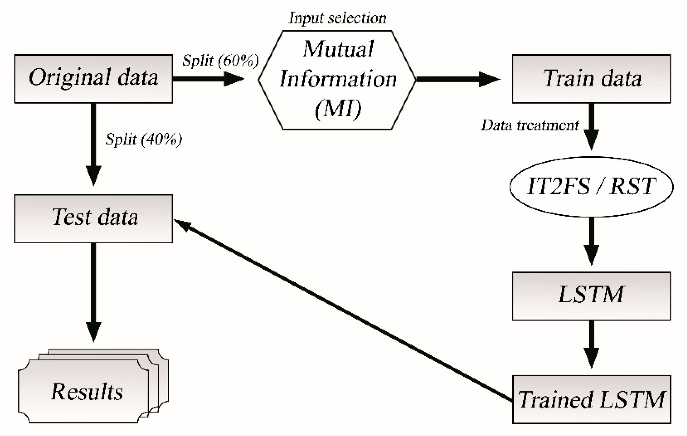
2. Materials and Methods

2.1. Dataset

A wind measurement station in Bandar-Abbas City, located at an international airport on Iran’s southern coast, is selected and wind speed data are retrieved from the Iran Meteorological Organization. In this case study, wind dataset contains wind speed data in 60-min (1 h) intervals for 3 years from 2016 to 2019. Given the possible seasonal behavior of wind speed data, ideally, more than one year should be used in the training set and use the remaining data for testing. In order to assess the proposed models and prevent overfitting, the 2016/01-2017/09 data are considered as the training (60% of datasets) and validation set, and the 2017/09-2019/01 data are considered as a testing set (40% of datasets).

Wind Characteristics

The meso-scale structure of the near-surface atmospheric conditions over the Persian Gulf are characterized by low-level winds with a single, coherent, land–sea breeze [32]. Wind speed data for 10m height was obtained from airport station. While southern winds are the predominant direction in the area, the average hourly wind speed in Bandar Abbas does not vary significantly throughout the year, with the maximum speed reaching 18–21 knots.

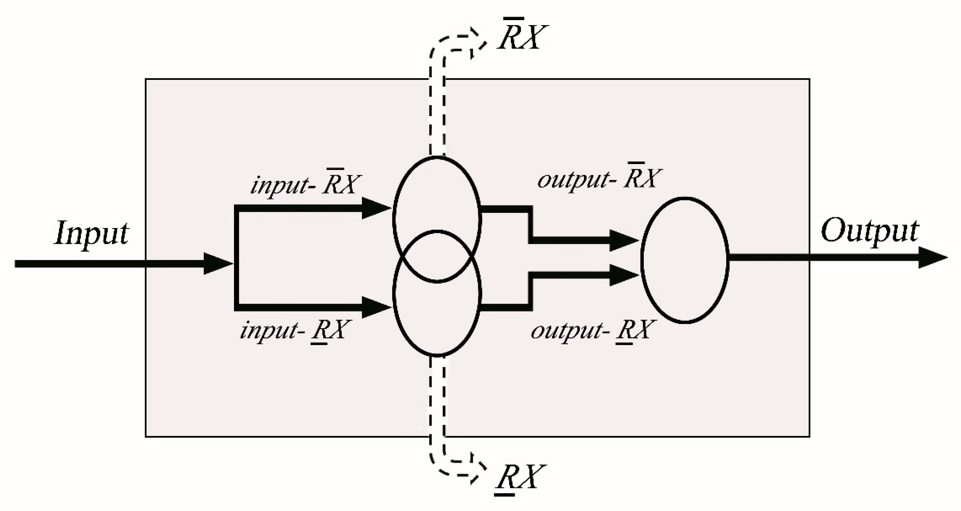
2.2. Rough Set Theory (RST)

The rough set was proposed in 1982 by Pawlak [33]. With the key principle of acquiring the characteristics of decision making or classification rules for problems by unchanging the ability to identify and using information reduction. The rough set theory has since been successfully applied in various disciplines [34,35] as one of the most powerful mathematical methods for dealing with ambiguity and vagueness and increases the performance of the predictor itself [36].
In this method, the key objectives are attribute reduction, correlation analysis, and significance assessment for ambiguous information systems using indiscernibility relationships to approximately approach the set of object through upper and lower approximations [37].
Suppose U is the nonempty universe with finite members; R is the equivalence relation in U; therefore, the knowledge base can be presented as a relation system K = (U, R). For the subset PR and Pϕ, the intersection of all the equivalence relation between 𝑃 can be called P-indiscernibility relation, defined by IND(P):
[ x ] I N D ( P ) = R P [ X ] R ,
where [ X ] R represents the equivalence class containing 𝑥∈U in relation R. Basic concepts of rough set theory are lower and upper approximations, which help to quantify the description of uncertain information. Suppose X is the subset of U; then, the lower approximation R _ X and upper approximation R ¯ X are
R _ X = { x U : [ x ] R X } ,
R ¯ X = { x U : [ x ] R X = ø } .
The boundary region BN R ( X ) = R ¯ X   R _ X , meanwhile, contains of those objects that cannot be classified with certainty as members of X with the knowledge in R. If BN R ( X )     ø , it indicates that R ¯ X     R _ X , and X cannot be represented by the equivalence class of R precisely. The set X is then called “rough” (or “roughly definable”); otherwise, X is crisp [38]. Figure 1 shows a schematic representation of RST.

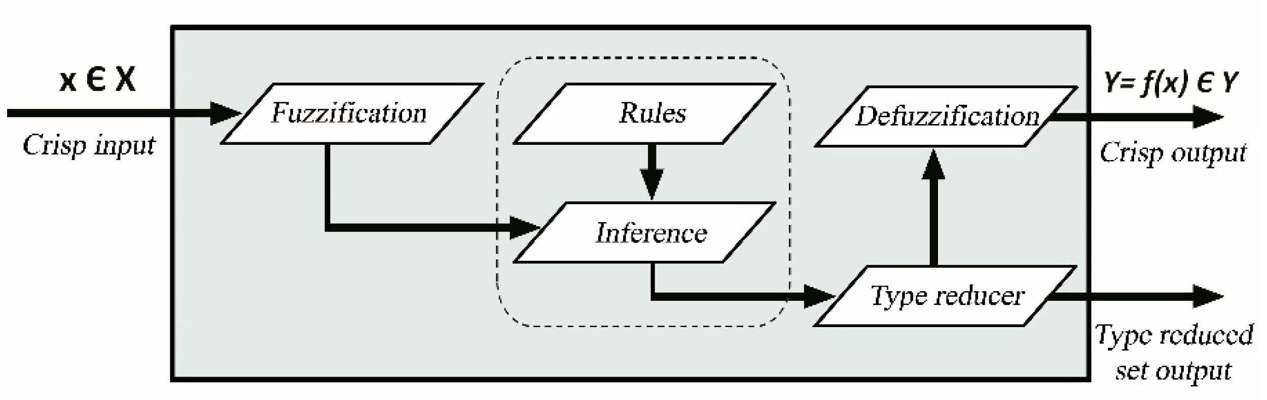
2.3. Interval Type-2 Fuzzy Sets

The definition of type-n fuzzy sets was proposed by Zadeh in 1975 [39], followed by the definition of type-2 fuzzy sets in 1976 [40]. Unlike classical set theory, where an element must necessarily belong to a set or not, an element can belong to a set to a certain degree (0 ≤ k ≤ 1) in the fuzzy set approach. Fuzzy set theory and its applications extensively developed over last years and attracted attention of practitioners, researchers and decision makers [41].
Li and Huang have presented relatively new definitions for type 2 fuzzy sets [42] and since then, fuzzy sets capability to capture data uncertainty, especially type 2 fuzzy sets, has been one of the most common directions in artificial and computational intelligence [43,44,45]. The type-2 fuzzy set is capable of dealing with uncertainties due to its ability to model them and reduce their impacts. This type of uncertainty is called ‘fuzzy uncertainty’. In contrast to ‘probabilistic’ uncertainty, which ‘relates to events with well-defined, unambiguous data,’ non-probabilistic or fuzzy uncertainty deals with ambiguities that often rely on qualitative details. Due to the lack of common numerical criteria for determining susceptibility, as well as the absence of “sharp” boundaries between susceptibility and non-susceptibility, mathematical models of susceptibility are difficult to derive. A benefit of using fuzzy set theory is that it enables the creation of inference models that express uncertainty using “natural language” [46].
Centroid, cardinality, fuzziness, variance and skewness are known as measurements of uncertainty for interval type-2 fuzzy sets (IT2FSs) [47]. The distinction between type-1 and type-2 fuzzy systems, having the same basic concept, is related to the type of fuzzy set applied. The IT2 fuzzy membership function is defined as follows for the discrete universe of discourse x and u [48]:
A ˜ = x X u J μ A ˜ ( x , u ) / ( x , u )
in which J x [ 0 , 1 ] is the first membership function of x. The case of μ A ˜ ( x , u ) = 1 ,   u   J x [ 0 , 1 ] is an interval type membership function. Consequently, an interval is the membership grade of each element of an IT2 fuzzy set. Uncertainty is characterized by the interval (commonly known as the footprint of uncertainty (FOU)) bounded by the upper (UMF) and lower (LMF) (Type-1) membership functions (MF). This secondary membership function determines the possibilities of the first MF. As can be seen in Figure 2, the IT2FS scheme is similar to the normal fuzzy scheme. Only the defuzzification mechanism is different, as it includes a type reducer block that converts the IT2 output set to a Type-1 set prior to performing a defuzzification step. In fact, type reduction is a phase in the process of defuzzifying type-2 fuzzy sets. Defuzzification of a type-2 fuzzy set consists of two steps: (a) type-reduction of the type-2 fuzzy set, which is the process of converting the type-2 fuzzy set to a type-1 fuzzy set, referred to as the type-reduced set (TRS); and (b) defuzzification of the type-1 fuzzy set, which is the process of defuzzing the TRS to obtain a crisp number, referred to as the type-2 fuzzy set’s centroid [49]. A more detailed summary is available elsewhere [50,51].

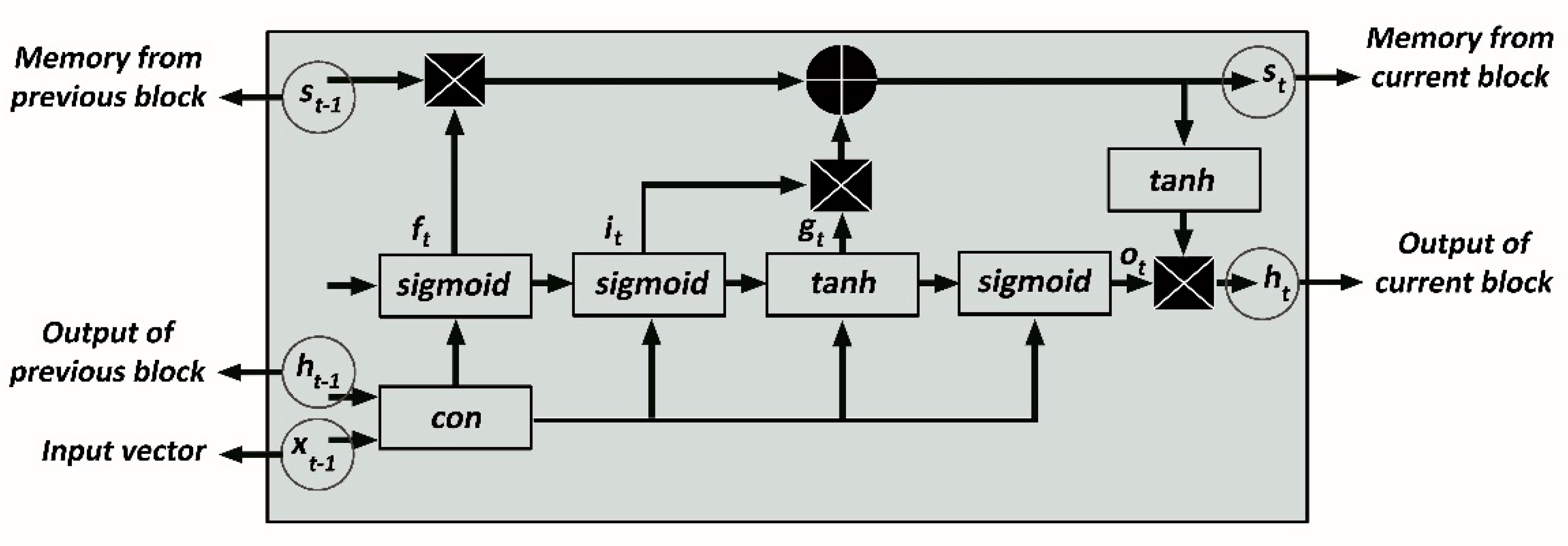
2.4. Long Short-Term Memory (LSTM) Network

In 1997, the Long-Short-Term Memory (LSTM) Network, a version of the RNN, was proposed [52] to build large recurring networks that can, in turn, be used to tackle difficult sequence problems in machine learning and achieve state-of-the-art outcomes. The basic unit of the hidden layer of LSTM, unlike traditional neural networks, is the memory block [53], which includes memory cells with self-connections that memorize the temporal state, and a pair of adaptive, multiplicative gating units that control information flowing into the block (Figure 3). As an input and output gate, two additional gates control the input and output activations in the block [21]. Due to the LSTM’s specific structure, it is capable of effectively resolving the gradient disappearance and explosion problems that occur during the RNN training procedure [54]. In Figure 3, the plus sign indicates that element levels are being added, the multiplication sign indicates that element levels are being multiplied, and the con indicates that vectors are being merged. The forgotten gate, input gate, input node, and output gate, respectively, are presented by f t , i t , g t , and o t . The relationship of the dependencies between the data in the input sequence is captured by the cell.
While the input gate regulates the volume of data that enters the cell, the forget gate regulates the amount of data that remains in the cell. The values in the cell are used to calculate the LSTM’s output activation; their extent is determined by the output gate. The LSTM structure’s calculation formulas are shown in Figure 3:
f t = σ ( W f [ h t 1 , x t ] + b f )
i t = σ ( W i [ h t 1 , x t ] + b i )
g t = t a n h ( W g [ h t 1 , x t ] + b g )
o t = σ ( W o [ h t 1 , x t ] + b o )
s t = s t 1 f t + g t i t
h t = tan h ( s t ) o t  
In Equations (6)–(11), W f , W i , W g , W o are the corresponding weight matrix connecting the input signal [ h t 1 , x t ] , and represents the element level multiplication. σ is the function of sigmoid activation, and tan h describes the hyperbolic tangent function. The state ( s t ) of cell remembers previous values over arbitrary time intervals and the three gates control the flow of information into and out of the cell.
Therefore, the LSTM network is very appropriate for prediction problems based on a time sequence [54]. The overall flowchart of the methodology has been depicted in Figure 4.

2.5. Evaluation Criteria

Performance of the proposed models were evaluated considering the uncertainties in model outputs using model evaluation criterial. The sum of squares error (SSE) and relative error (RE) are used as two evaluation metrics
S S E = t = 1 N [ y ^ ( t ) y ( t ) ] 2
R E = | y ( t ) y ^ ( t ) | | y ^ ( t ) | 100 %
where, y ^ ( t ) and y ( t ) are the predicted and measured output, respectively.
The optimal model is selected based on the minimum statistical error.

3. Results and Discussion

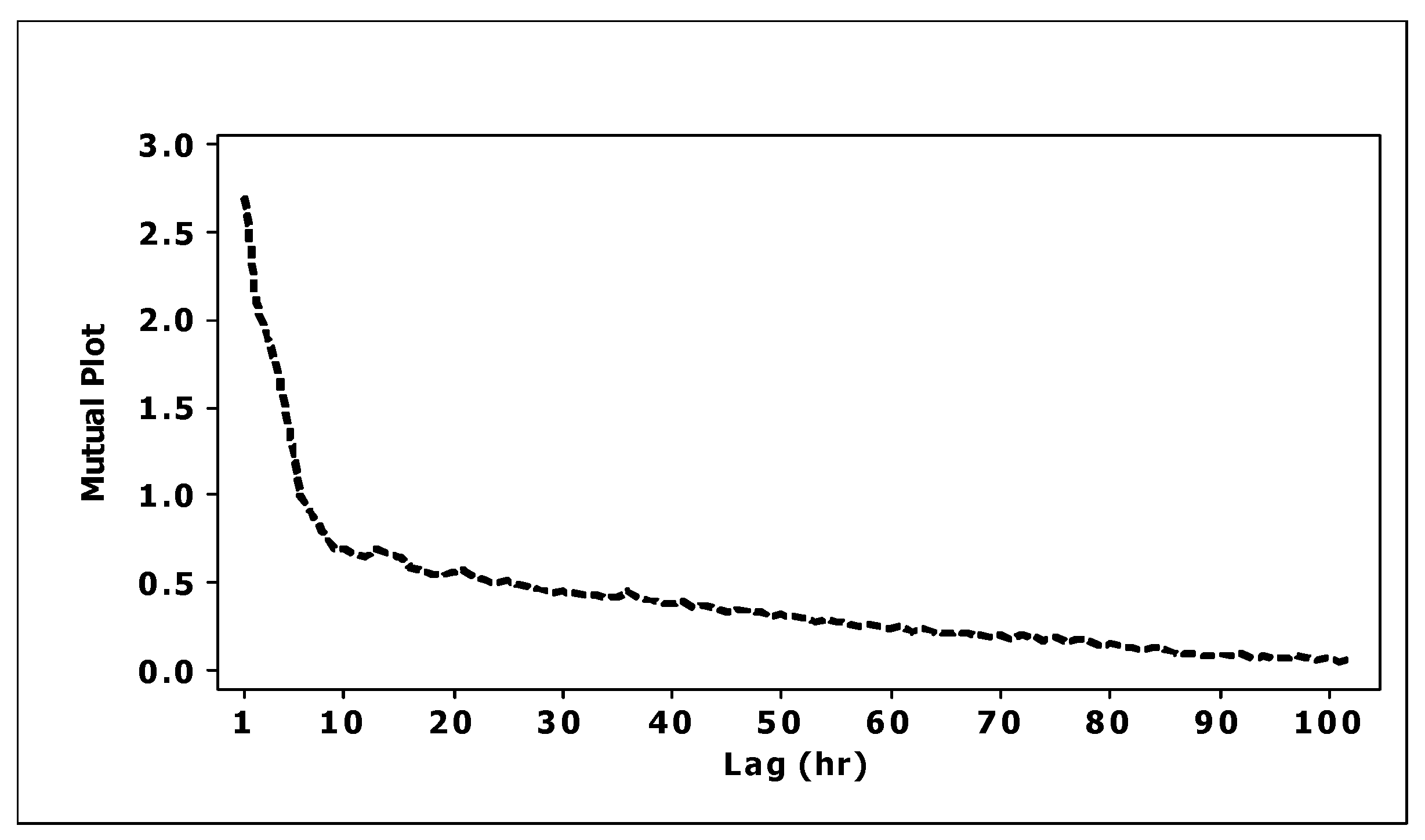
3.1. Selection of Input Variable

The selection of input variables is a critical step in deciding the optimal structure of data-driven models. The wind speed time series in this case exhibits excessive variability (Figure 5), and linear regression does not function well for forecasting because the time series is nonlinear [55].
Several papers [56] have used the autocorrelation function (ACF) to determine the cross-correlation of a time series with itself at different points in time. Due to the fact that ACF quantifies a variable’s linear dependence on itself and wind speed is a nonlinear time series, mutual knowledge (MI) is used to efficiently test both linear and nonlinear correlations.
MI’s objective is to determine the stochastic dependency between two random variables without making any assumptions about their relationship’s nature (e.g., linearity) [57]. In other words, MI evaluates the dependencies between random variables, where each variable contains information about the other [58].
The basic idea behind a variable selection algorithm based on MI is to maximize the joint MI between the subset and the target output [59]. Battiti [60] used MI in data analysis and presented feature selection algorithm based on this measure. An MI-based input selection algorithm was used by Rashidi Khazaee et al. [61] to select the proper inputs for the prediction model, demonstrated that the proposed input selection model, can efficiently select relevant input variables.
Although detailed description of the MI technique can be found elsewhere [62], portions of which are provided here to help elaborate the technique. MI between two random variables x and y is described as [63]
I ( x ; y ) = p ( x , y ) l o g p ( x , y ) p ( x ) p ( y ) d x   d y
where the probability density functions of X and Y are p(x) and p(y), the joint probability density function of X and Y is p(x,y). The joint probability density p(x,y) will be equal to the product of probability densities in the case of no dependence between two variables, so the MI is equal to zero.
The MI of v(t − l + 1) and v(t + 1) is calculated using l as the time lag, and v(t) as the wind speed time series value at time t. Figure 6 illustrates the MI for lags ranging from 1 to 100. The correlation between wind speed measurements decreases as the time lag increases.
The product of input variable selection using MI for the dataset results in an 81-dimensional input vector that is fed to the suggested deep learning models. After each training epoch, the trained model’s output is evaluated by calculating the model’s performance on an unseen data set using the validation set data. Although there are no criteria for the percentage of data used in the validation and training phases, the decrease in validation errors during the training process shows that overfitting is avoided [64]. To address the correlation in the wind speed data, the input set includes wind speed values corresponding to time lags with MI greater than = 0.35.

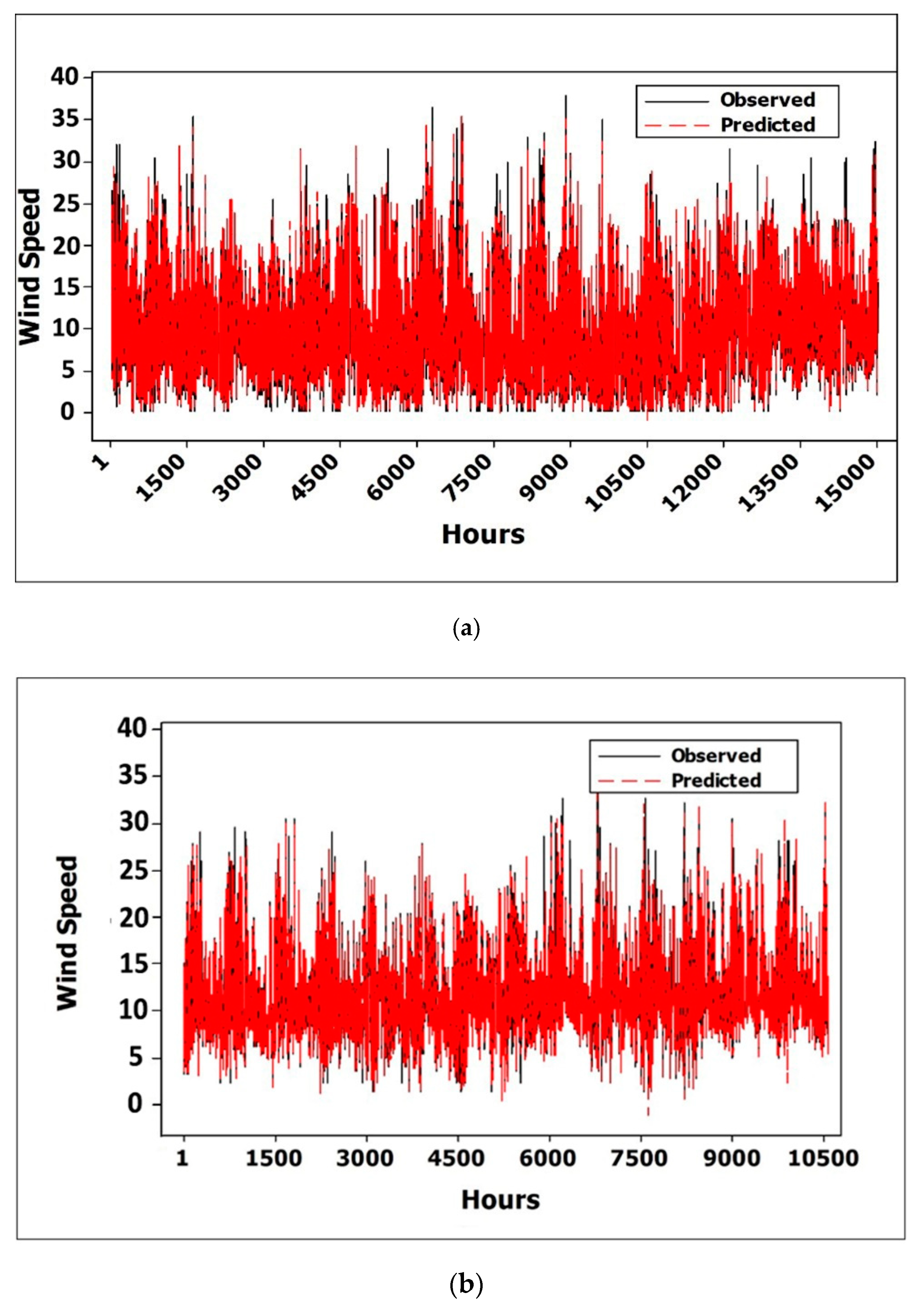
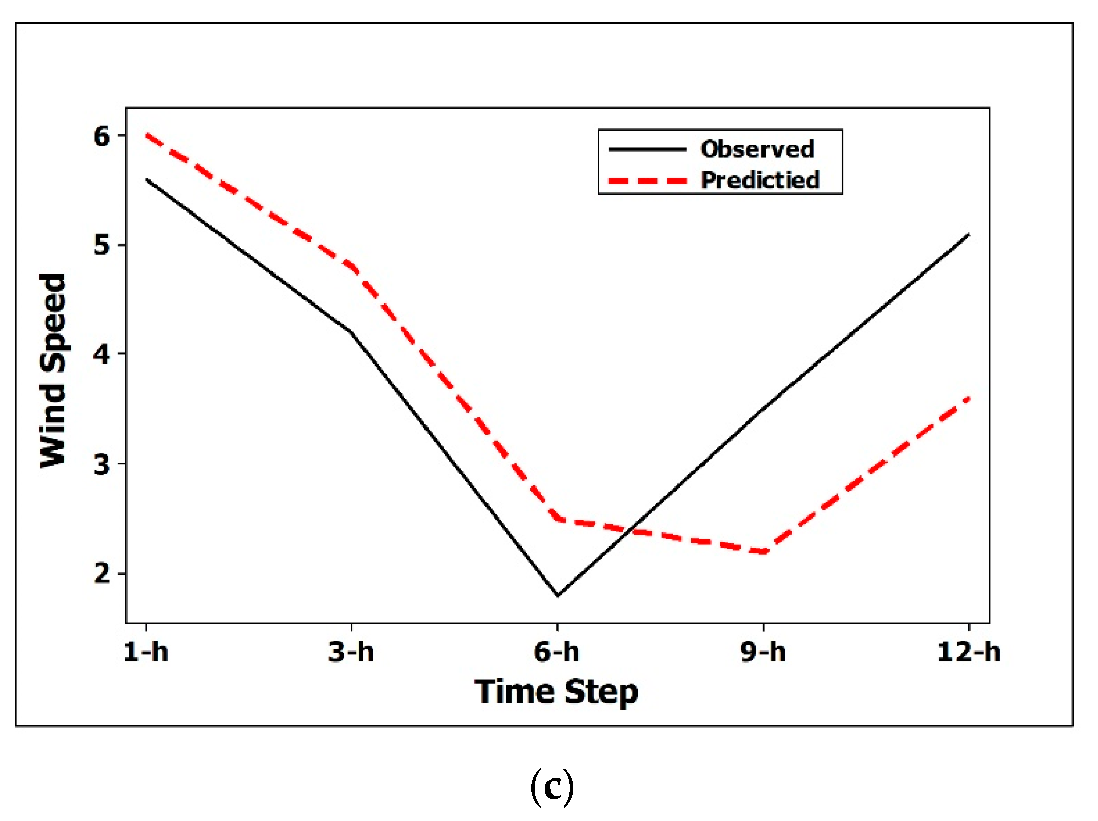
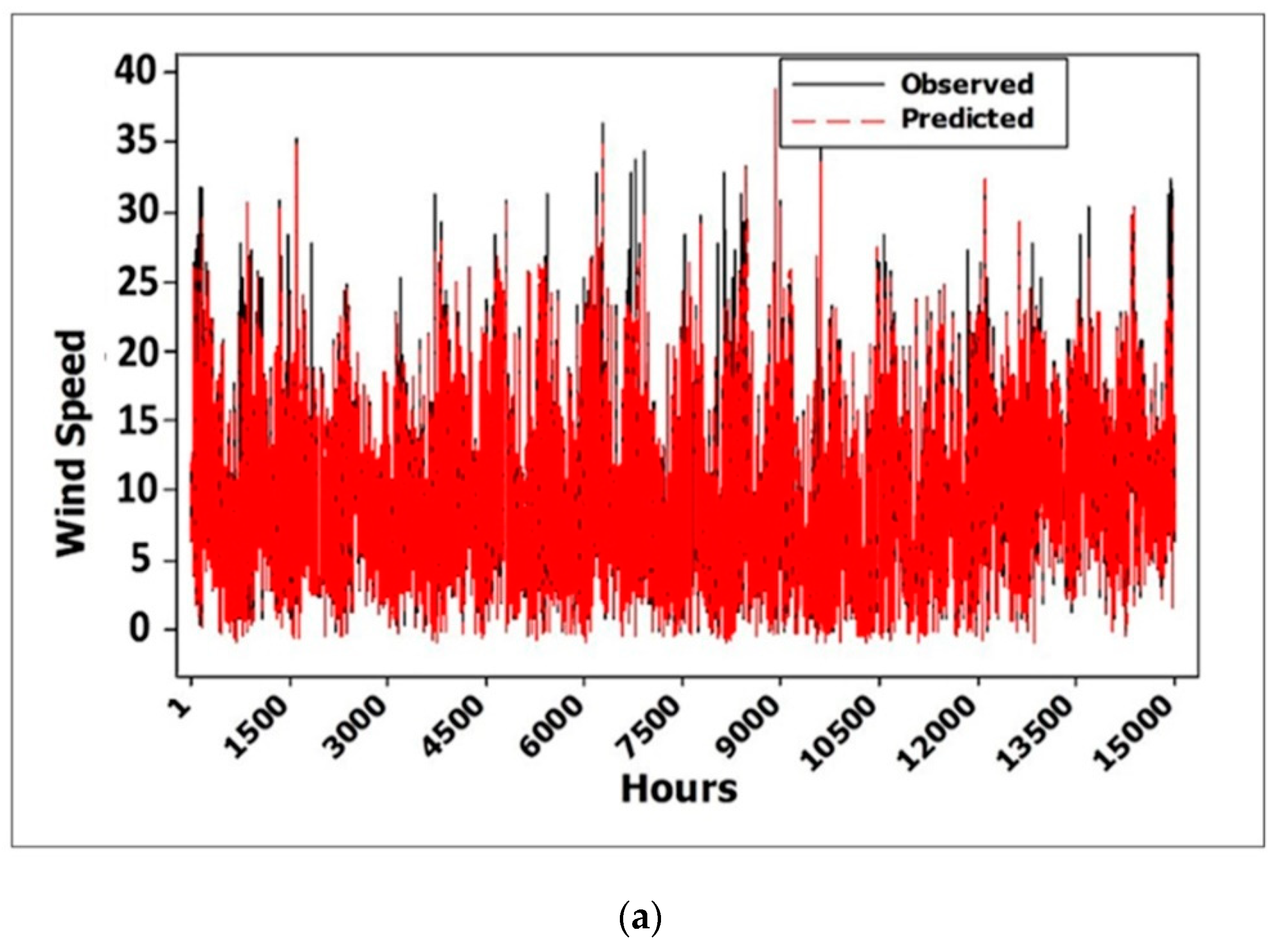
3.2. Wind Speed Forecasting Models

The RST/FST generated decision rule was provided as input to the LSTM. The LSTM analyzes the attributes of the data with decision rule for wind speed prediction. It means that the features selected by the RST/FST are provided as input to the LSTM for the analysis.
Through the simulation experiment, the predicted wind speed data using RST-LSTM is shown in Figure 7. The black line is the observed data of wind speed, and the dashed red is the predicted data. The optimal structure is calculated by test simulation calculations amongst the observed and predicted datasets, where the LSTM prediction model comprises of an 81-node input layer, a 25-node hidden layer, and a 1-node output layer, RST-LSTM (81-25-1), with a minimum RE of 0.065 and 0.085 during the training and testing phases, respectively.
The most accurate IT2F-LSTM model is demonstrated with 81-15-1 network structure and Relative Error of 0.074 and 0.088 during training and testing periods, respectively (Figure 8).
With RST-LSTM being slightly superior, estimates from both RST-LSTM and IT2F-LSTM models are close to the attributed observed wind speed variations possibly due to the application of highly correlated input data with less uncertainty for these models. In terms of curve fitting, the curve of the predicted data in both models is very similar to the curve of the actual data. In spite of the certain deviation of the crests and troughs in training and testing, due to the uneven occurrence of data, there is a perfect predictability in other locations.
Throughout the training and testing phases of the 1 h ahead prediction interval, the majority of the points were placed along the diagonal line based on the scatterplots of the observed versus predicted wind speed time series produced by both the RST-LSTM and IT2F-LSTM models (Figure 9a–d). The prediction results of the proposed models were, therefore, in good agreement with the corresponding wind speeds measured.
The modeling results were compared with the original LSTM (Figure 10), multilayer neural networks (MLNN), and recurrent neural network (RNN) models (Table 1) in order to assess the prediction performance of the proposed models, using the same input combinations as those used in the RST-LSTM and IT2F-LSTM models.
The overall results indicate that the RNN, MLNN, and original LSTM models cannot surpass the performance of the improved RST-LSTM and IT2F-LSTM models in wind speed prediction (Table 1 and Table 2). The RST-LSTM model demonstrates the best performance, with lowest SSE (Sum of Squares Error) and RE (Relative Error) of training and testing datasets for different time steps.
The best structures of the prediction models developed in this study is shown in Table 3. As can be seen in Table 3, the best performance having the lowest error was observed for the 1 h ahead prediction for all proposed models presenting RST-LSTM (81-25-1) the most capable deep learning model to satisfactory estimate the overall behavior and accurately predict the short-term variations of the wind speed series.
RST-LSTM networks have the benefits of optimizing the selection and determining the significance of the variables affecting the dataset’s internal relationships. This method overcomes the disadvantages of quantitative interpretation of intelligent prediction models and guarantees the objectivity of prediction model analysis [65].
In addition, compared to traditional neural networks, the benefit of the LSTM is its ability to learn long-term dependencies between the supplied network input and output, which are important for modeling difficult sequence issues with excessive fluctuations and achieving state-of-the-art outcomes. In terms of uncertainty incorporation, the main advantage of rough set theory is that it does not require any preliminary or supplementary knowledge about the data, such as necessary probability distributions in statistics, basic probability assignments in evidence theory, a grade of membership or the value of possibility needed in fuzzy set theory [66].
Although the performance of both RST-LSTM and FST-LSTM models is superior to that of the traditional neural network prediction approaches, the inter-comparison of the obtained results shows that the RST-LSTM model outperforms the FST-LSTM model in wind speed forecasting. Benefited from efficient variable input selection using mutual information, RST-LSTM with the property of pattern remembrance can be further applied by managers and decision makers to conduct better and more effective wind speed predictions and fill in the gaps between power generation and power utilization. It can help with the smooth operation of the power system as well as the optimization of the control strategy. Variables uncertainty that influence wind speed are reduced by the fuzzy rough set theory, which simplifies the input of the neural network prediction model and improves accuracy and speed.

4. Conclusions

In providing renewable and clean energy alternatives, wind power generation is playing an increasingly important role. The intermittency and stochastic nature of wind speed, however, makes its prediction a difficult issue for the construction and management of wind farms. Precise wind speed forecasting is, therefore, very critical for the efficient operation and planning of large-scale wind turbine integration. In this paper, the framework of deep learning is applied in the prediction of wind speed using LSTM model hybridized with rough (RST-LSTM) and fuzzy set theory (FST-LSTM) to generate more accurate model with efficient prediction. The short-term wind speed forecasting model is an important contribution for reliable large-scale wind power forecasting and integration in areas influenced by Mediterranean wind. Moreover, since wind speed is a nonlinear time series, unlike many other studies that applied ACF to measure a variable’s linear dependency, an efficient method of MI is used here for input variable selection to evaluate excessive fluctuations of wind speed time series, both linear and nonlinear correlations.

Author Contributions

M.I.: writing original draft, writing—review and editing, methodology; H.F.: writing—original draft, writing—review and editing; W.-H.L.: writing—review and editing, formal analysis, investigation, validation; H.-C.K.: formal analysis, writing—review and editing; C.M.L.: formal analysis, writing—review and editing; Y.-S.H.: formal analysis, writing—review and editing; C.-Y.K.: writing—review and editing, supervision. All authors have read and agreed to the published version of the manuscript.

Funding

This research was funded by the Ministry of Science and Technology of Taiwan (MOST), with grant numbers of 109-2811-E-006 -522 -, 107-2221-E-006 -124 -MY3, 108-2621-M-006 -005 -, and 108-2621-M-309 -001 -MY2.

Institutional Review Board Statement

Not applicable.

Informed Consent Statement

Not applicable.

Data Availability Statement

The data that support the findings of this study are available from the corresponding author upon reasonable request.

Conflicts of Interest

The authors declare no conflict of interest.

References

  1. Oyedepo, S.O.; Adaramola, M.S.; Paul, S.S. Analysis of wind speed data and wind energy potential in three selected locations in south-east Nigeria. Int. J. Energy Environ. Eng. 2012, 3, 7. [Google Scholar] [CrossRef] [Green Version]
  2. Foley, A.M.; Leahy, P.G.; Marvuglia, A.; McKeogh, E.J. Current methods and advances in forecasting of wind power generation. Renew. Energy. 2012, 37, 1–8. [Google Scholar] [CrossRef] [Green Version]
  3. Chen, J.; Zeng, G.Q.; Zhou, W.; Du, W.; Lu, K.D. Wind speed forecasting using nonlinear-learning ensemble of deep learning time series prediction and extremal optimization. Energy Convers. Manag. 2018, 165, 681–695. [Google Scholar] [CrossRef]
  4. Cassola, F.; Burlando, M. Wind speed and wind energy forecast through Kalman filtering of Numerical Weather Prediction model output. Appl. Energy. 2012, 99, 154–166. [Google Scholar] [CrossRef]
  5. Chen, L.; Li, Z.; Zhang, Y. Multiperiod-Ahead Wind Speed Forecasting Using Deep Neural Architecture and Ensemble Learning. Math. Probl. Eng. 2019, 9240317. [Google Scholar] [CrossRef]
  6. Jung, J.; Broadwater, R.P. Current status and future advances for wind speed and power forecasting . Renew. Sustain. Energy Rev. 2014, 31, 762–777. [Google Scholar] [CrossRef]
  7. Khodayar, M.; Wang, J. Spatio-Temporal Graph Deep Neural Network for Short-Term Wind Speed Forecasting. IEEE Trans. Sustain. Energy 2019, 10, 670–681. [Google Scholar] [CrossRef]
  8. Wang, H.; Liu, D.; Wang, J.L. Ultra-Short-Term Wind Speed Prediction Based on Spectral Clustering and Optimized Extreme Learning Machine. Power Syst. Technol. 2015, 5, 1307–1314. [Google Scholar]
  9. Zeng, J.; Zhang, H. A Wind Speed Forecasting Model Based on Least Squares Support Vector Machine. Power Syst. Technol. 2009, 18, 144–147. [Google Scholar]
  10. Tascikaraoglu, A.; Uzunoglu, M. A review of combined approaches for prediction of short-term wind speed and power. Renew. Sustain. Energy Rev. 2014, 34, 243–254. [Google Scholar] [CrossRef]
  11. Twain, M. Wind Power Forecasting. In Valuing Wind Generation on Integrated Power Systems; Elsevier Inc.: Amsterdam, The Netherlands, 2010; pp. 87–99. [Google Scholar]
  12. Chang, G.; Lu, H.; Chang, Y.; Lee, Y. An improved neural network-based approach for short-term wind speed and power forecast. Renew. Energy 2017, 105, 301–311. [Google Scholar] [CrossRef]
  13. Noorollahi, Y.; Jokar, M.A.; Kalhor, A. Using artificial neural networks for temporal and spatial wind speed forecasting in Iran. Energy Convers. Manag. 2016, 115, 17–25. [Google Scholar] [CrossRef]
  14. Imani, M.; You, R.J.; Kuo, C.Y. Caspian Sea level prediction using satellite altimetry by artificial neural networks. Int. J. Environ. Sci. Technol. 2014, 11, 1035–1042. [Google Scholar] [CrossRef] [Green Version]
  15. Wang, H.; Li, G.; Wang, G.; Peng, J.; Jiang, H.; Liu, Y. Deep learning based ensemble approach for probabilistic wind power forecasting. Appl. Energy 2017, 188, 56–70. [Google Scholar] [CrossRef]
  16. Qureshi, A.S.; Khan, A.; Zameer, A.; Usman, A. Wind power prediction using deep neural network based meta regression and transfer learning. Appl. Soft Comput. 2017, 58, 742–755. [Google Scholar] [CrossRef]
  17. Lv, Y.; Duan, Y.; Kang, W.; Li, Z.; Wang, F. Traffic flow prediction with big data: A deep learning approach. IEEE Trans. Intell. Transp. Syst. 2014, 16, 865–873. [Google Scholar] [CrossRef]
  18. Qiu, X.; Ren, Y.; Suganthan, P.N.; Amaratunga, G. Empirical mode decomposition based ensemble deep learning for load demand time series forecasting. Appl. Soft Comput. 2017, 54, 246–255. [Google Scholar] [CrossRef]
  19. Hu, Q.; Zhang, R.; Zhou, Y. Transfer learning for short-term wind speed prediction with deep neural networks. Renew. Energy 2016, 85, 83–95. [Google Scholar] [CrossRef]
  20. Wang, H.; Wang, G.; Li, G.; Peng, J.; Liu, Y. Deep belief network based deterministic and probabilistic wind speed forecasting approach. Appl. Energy 2016, 182, 80–93. [Google Scholar] [CrossRef]
  21. Li, R.; Hu, Y.; Liang, Q. T2F-LSTM Method for Long-term Traffic Volume Prediction. IEEE Trans Fuzzy Syst. 2020, 28, 3256–3264. [Google Scholar] [CrossRef]
  22. Huang, Y.; Zhao, H.; Huang, X. A Prediction Scheme for Daily Maximum and Minimum Temperature Forecasts Using Recurrent Neural Network and Rough set. IOP Conf. Ser. Earth Environ. Sci. 2019, 237, 022005. [Google Scholar] [CrossRef]
  23. Ma, X.L.; Tao, Z.M.; Wang, Y.H. Long short-term memory neural network for traffic speed prediction using remote microwave sensor data. Transp. Res. Part C Emerg. Technol. 2015, 54, 187–197. [Google Scholar] [CrossRef]
  24. Liu, Y.P.; Zheng, H.F.; Feng, X.X. Short-term traffic flow prediction with Conv-LSTM. In Proceedings of the International Conference on Wireless Communications & Signal Processing, Nanjing, China, 11–13 October 2017; pp. 1–6. [Google Scholar]
  25. Yang, B.B.; Yin, K.L.; Du, J. Dynamic prediction model of landslide displacement based on time series and long and short time memory networks. Chin. J. Rock Mech. Eng. 2018, 37, 2334–2343. [Google Scholar]
  26. Liu, Y.X.; Fan, Q.X.; Shang, Y.Z.; Fan, Q.M.; Liu, Z.W. Short-term water level prediction method for hydropower stations based on LSTM neural network. Adv. Sci. Technol. Water Resour. 2019, 39, 56–60. [Google Scholar]
  27. Beaubouef, T.; Petry, F.E. Fuzzy and Rough Set Approaches for Uncertainty in Spatial Data. In Studies in Fuzziness and Soft Computing; Jeansoulin, R., Ed.; Springer-Verlag: Berlin/Heidelberg, Germany, 2010; Volume 256, pp. 103–129. [Google Scholar]
  28. Mostafaeipour, A.; Mostafaeipour, N. Renewable energy issues and electricity production in Middle East compared with Iran. Renew. Sust. Energ. Rev. 2009, 13, 1641–1645. [Google Scholar] [CrossRef]
  29. Shabaniverki, M.; Shabaniverki, H.; Babapoor, H.; Banisaffar, M. An Overview of Wind and Solar Energies in Iran. In Proceedings of the 1st Technical Seminar on the Role of New Technologies in Protecting Environment Faculty of New Sciences & Technologies, University of Tehran, Tehran, Iran, 17 February 2015. [Google Scholar]
  30. Hadipour, V.; Vafaie, F.; Lan, W.H.; Kerle, N. An indicator-based approach to assess social vulnerability of coastal areas to sea-level rise and flooding: A case study of Bandar Abbas city, Iran. Ocean Coast Manag. 2020, 188, 105077. [Google Scholar] [CrossRef]
  31. Renewable Energy and Energy Efficiency Organization. Available online: http://www.satba.gov.ir/en/home (accessed on 28 February 2021).
  32. Zhu, M.; Atkinson, B.W. Observed and modelled climatology of the land–sea breeze circulation over the Persian Gulf. Int. J. Climatol. 2004, 24, 883–905. [Google Scholar] [CrossRef]
  33. Pawlak, Z. Rough sets. Int. J. Comput. Inf. Sci. 1982, 11, 341–346. [Google Scholar] [CrossRef]
  34. Wang, S.; Wang, W.; Sun, W.; Zhang, K. Short-Term Load Forecasting of Micro Grid Based on Rough Sets and BP Neural Network. Control Eng. China 2018, 25, 1528–1533. [Google Scholar]
  35. Chen, S.; Wu, A.; Wang, Y.; Chen, X. Rock Mass Quality Evaluation Based on Rough Set and Improved Efficacy Coefficient Method. J. Huazhong Uni. Sci. Technol. 2018, 46, 36–41. [Google Scholar]
  36. Durairaj, M.; Meena, K. A Hybrid Prediction System Using Rough Sets and Artificial Neural Networks. IJITEE 2011, 1, 16–23. [Google Scholar]
  37. Stefanowski, J. On rough set based approaches to induction of decision rules. Rough Sets Knowl. Discov. 1998, 1, 500–529. [Google Scholar]
  38. Niu, D.; Ji, L.; Ma, Q.; Li, W. Knowledge Mining Based on Environmental Simulation Applied to Wind Farm Power Forecasting. Math. Probl. Eng. 2013, 597562. [Google Scholar] [CrossRef] [Green Version]
  39. Zadeh, L. The concept of a linguistic variable and its application to approximate reason-1. Inf. Sci. 1975, 8, 199–249. [Google Scholar] [CrossRef]
  40. Mizumoto, M.; Tanaka, K. Some properties of fuzzy sets of type-2. Inf. Control 1976, 31, 312–340. [Google Scholar] [CrossRef] [Green Version]
  41. Pawlak, Z. Rough Sets; University of Information Technology and Management ul: Warsaw, Poland, 1982; p. 51. [Google Scholar]
  42. Li, Y.M.; Huang, J. Type-2 fuzzy mathematical modeling and analysis of the dynamical behaviors of complex ecosystems. Simul. Model. Pract. Th. 2008, 16, 1379–1391. [Google Scholar]
  43. Li, R.M.; Jiang, C.Y.; Zhu, F.H. Traffic flow data forecasting based on Interval Type-2 Fuzzy Sets theory. J. Auto. Sinica 2016, 2, 141–148. [Google Scholar]
  44. Zhao, H.; Wang, P.; Hu, Q.H. Fuzzy rough set based feature selection for large-scale hierarchical classification. IEEE Trans Fuzzy Syst. 2018, 27, 1891–1903. [Google Scholar] [CrossRef]
  45. Greenfield, S.; Chiclana, F. Defuzzification of the discretized generalized type-2 fuzzy set: Experimental evaluation. Inf. Sci. 2013, 244, 1–25. [Google Scholar] [CrossRef] [Green Version]
  46. Eierdanz, F.; Alcamo, J.; Acosta-Michlik, L.; Krömker, D.; Tänzler, D. Using fuzzy set theory to address the uncertainty of susceptibility to drought. Reg. Environ. Chang. 2008, 8, 197–205. [Google Scholar] [CrossRef]
  47. Wu, D.; Mendel, J.M. Uncertainty measures for interval type-2 fuzzy sets. Inf. Sci. 2007, 177, 5378–5393. [Google Scholar] [CrossRef]
  48. Castillo, O.; Melin, P. Type-2 Fuzzy Logic: Theory and Applications. Stud. Fuzziness Soft Comput. 2008, 223. [Google Scholar] [CrossRef]
  49. Mendel, J.M. Uncertain Rule-Based Fuzzy Logic Systems: Introduction and New Directions. PrenticeHall PTR 2001. [Google Scholar] [CrossRef]
  50. Castillo, O. Type-2 Fuzzy Logic in Intelligent Control Applications. Stud. Fuzziness Soft Comput. 2012, 272. [Google Scholar] [CrossRef]
  51. Mendel, J.M. Uncertain Rule-Based Fuzzy Systems. Introduction and New Directions, 2nd ed.; Springer International Publishing AG: Basel, Switzerland, 2017. [Google Scholar]
  52. Hochreiter, S.; Schmidhuber, J. Long short-term memory. Neural Comput. 1997, 9, 1735–1780. [Google Scholar] [CrossRef] [PubMed]
  53. Abigogun, O.A. Data Mining, Fraud Detection and Mobile Telecommunications: Call Pattern Analysis with Unsupervised Neural Networks. Master’s Thesis, University of the Western Cape, Greater Cape Town, South Africa, 2005. [Google Scholar]
  54. Liu, Y.; Guan, L.; Hou, C.; Han, H.; Liu, Z.; Sun, Y.; Zheng, M. Wind Power Short-Term Prediction Based on LSTM and Discrete Wavelet Transform. Appl. Sci. 2019, 9, 1108. [Google Scholar] [CrossRef] [Green Version]
  55. Hu, Q.; Su, P.; Yu, D.; Liu, J. Pattern-based wind speed prediction based on generalized principal component analysis. IEEE Trans. Sustain. Energy 2014, 5, 866–874. [Google Scholar] [CrossRef]
  56. Imani, M.; Kao, H.C.; Lan, W.H.; Kuo, C.Y. Daily sea level prediction at Chiayi coast, Taiwan using extreme learning machine and relevance vector machine. Glob. Planet. Chang. 2018, 161, 211–221. [Google Scholar] [CrossRef]
  57. Steuer, R.; Kurths., J.; Daub., C.; Weise, J.; Selbig, J. The mutual information: Detecting and evaluating dependencies between variables. Bioinformatics 2020, 18, S231–S240. [Google Scholar] [CrossRef] [PubMed] [Green Version]
  58. May, R.; Dandy, G.; Maier, H. Review of Input Variable Selection Methods for Artificial Neural Networks. In Artificial Neural Networks—Methodological Advances and Biomedical Applications; Suzuki, K., Ed.; BoD—Books on Demand: Norderstedt, Germany, 2011; p. 362. [Google Scholar]
  59. Vergara, J.R.; Estévez, P.A. A review of feature selection methods based on mutual information. Neural Comput. Appl. 2014, 24, 175–186. [Google Scholar] [CrossRef]
  60. Battiti, R. Using mutual information for selecting features in supervised neural net learning. IEEE Trans Neural Netw. 1994, 5, 537–550. [Google Scholar] [CrossRef] [PubMed] [Green Version]
  61. Rashidi Khazaee, P.; Mozayani, N.; Jahed Motlagh, M.R. Mutual Information Based Input Variable Selection Algorithm and Wavelet Neural Network for Time Series Prediction. In Proceedings of the International Conference on Artificial Neural Networks, Berlin/Heidelberg, Germany, 15–18 September 2008. [Google Scholar]
  62. Rossi, F.; Lendasse, A.; Francois, D.; Wertz, V.; Verleysen, M. Mutual Information for the selection of relevant variables in spectrometric nonlinear modelling. Chemometr. Intell. Lab. 2006, 80, 215–226. [Google Scholar] [CrossRef] [Green Version]
  63. Darudi, A.; Rezaeifar, S.; Javidi Dasht Bayaz, M.H. Partial Mutual Information Based Algorithm for Input Variable Selection. In Proceedings of the 13th International Conference on Environment and Electrical Engineering (EEEIC), Wroclaw, Poland, 1–3 November 2013. [Google Scholar]
  64. Khodayar, M.; Kaynak, O.; Khodayar, M.E. Rough Deep Neural Architecture for Short-Term Wind Speed Forecasting. IEEE Trans. Ind. Inform. 2017, 13, 2770–2779. [Google Scholar] [CrossRef]
  65. Qu, X.; Yang, J.; Chang, M. A Deep Learning Model for Concrete Dam Deformation Prediction Based on RS-LSTM. J. Sens. 2019, 4581672. [Google Scholar] [CrossRef]
  66. Skowron, A.; Dutta, S. Rough sets: Past, present, and future. Nat Comput. 2018, 17, 855–876. [Google Scholar] [CrossRef] [PubMed] [Green Version]
Figure 1. A schematic representation of RST.
Atmosphere 12 00924 g001
Figure 2. A schematic representation of IT2 Fuzzy System.
Atmosphere 12 00924 g002
Figure 3. Schematic representation of long short-term memory (LSTM) unit structure.
Atmosphere 12 00924 g003
Figure 4. The flowchart of the proposed methodology and modeling strategy.
Atmosphere 12 00924 g004
Figure 5. Wind speed (km/h) time series fluctuations in the current study.
Atmosphere 12 00924 g005
Figure 6. Mutual information of various time-lags.
Atmosphere 12 00924 g006
Figure 7. Wind speed (km/h) forecasting analysis of RST-LSTM (81-25-1) during the (a) training, (b) testing, and (c) predicting periods.
Atmosphere 12 00924 g007aAtmosphere 12 00924 g007b
Figure 8. Wind speed (km/h) forecasting analysis of IT2F-LSTM (81-15-1) during the (a) training, (b) testing, and (c) predicting periods.
Atmosphere 12 00924 g008aAtmosphere 12 00924 g008b
Figure 9. The RST-LSTM (a,b) and IT2F-LSTM (c,d) scatter plots display the positive linear relation between the observed time series and the predicted value during the periods of training (a,c) and testing (b,d).
Atmosphere 12 00924 g009aAtmosphere 12 00924 g009b
Figure 10. Wind speed forecast using the LSTM model (81-14-1) during (a) training, and (b) testing periods, and scatter plots showing the positive linear correlation between the observed time series and the predicted values in (c) training, and (d) testing periods.
Atmosphere 12 00924 g010aAtmosphere 12 00924 g010b
Table 1. SEE (sum of squares error) of training and testing datasets using forecasting approaches for different time steps.
Training
Model
Time StepRST-LSTMMLNNIT2F-LSTMLSTMRNN
1 h103129112126141
3 h109138119132155
6 h123163131154166
9 h145174152167179
12 h161196176182201
Testing
Method
Time StepRST-LSTMMLNNIT2F-LSTMLSTMRNN
1 h130155136149161
3 h137164148155170
6 h169187174183189
9 h210236218229241
12 h245272251263277
Table 2. RE (relative error) of training and testing datasets using forecasting approaches for different time steps.
Training
Model
Time StepRST-LSTMMLNNIT2F-LSTMLSTMRNN
1 h0.0650.0870.0740.0890.099
3 h0.0720.0950.0830.0930.113
6 h0.0850.1130.0910.1120.119
9 h0.1030.1240.1100.1190.209
12 h0.1160.2260.2050.2130.230
Testing
Model
Time StepRST-LSTMMLNNIT2F-LSTMLSTMRNN
1 h0.0850.1060.0880.0960.109
3 h0.0990.1190.1050.1120.132
6 h0.1280.1530.1350.1410.159
9 h0.1490.2240.1520.2010.252
12 h0.1810.2760.1930.2700.281
Table 3. The best structures of the prediction models having lowest error.
Time Ahead
Model1 h3 h6 h9 h12 h
RNN81-28-181-33-181-35-181-37-181-29-1
LSTM81-14-181-13-181-14-181-16-181-13-1
IT2F-LSTM81-15-181-16-181-15-181-18-181-21-1
MLNN81-77-30-181-82-41-181-76-38-181-85-40-181-75-45-1
RST-LSTM81-25-181-29-181-30-181-20-181-18-1
Publisher’s Note: MDPI stays neutral with regard to jurisdictional claims in published maps and institutional affiliations.

