Article

On the Relationship of Cold Pool and Bulk Shear Magnitudes on Upscale Convective Growth in the Great Plains of the United States

by
Zachary A. Hiris
1 and
William A. Gallus, Jr.
2,*
1
NOAA/NWS, WSI, 325 Broadway, Boulder, CO 80305-3337, USA
2
Department of Geological & Atmospheric Sciences, Iowa State University, 3025 Agronomy, Ames, IA 50011, USA
*
Author to whom correspondence should be addressed.
Submission received: 19 July 2021 / Revised: 5 August 2021 / Accepted: 6 August 2021 / Published: 9 August 2021
(This article belongs to the Section Meteorology)

Abstract

:
Upscale convective growth remains a poorly understood aspect of convective evolution, and numerical weather prediction models struggle to accurately depict convective morphology. To better understand some physical mechanisms encouraging upscale growth, 30 warm-season convective events from 2016 over the United States Great Plains were simulated using the Weather Research and Forecasting (WRF) model to identify differences in upscale growth and non-upscale growth environments. Also, Bryan Cloud Model (CM1) sensitivity tests were completed using different thermodynamic environments and wind profiles to examine the impact on upscale growth. The WRF simulations indicated that cold pools are significantly stronger in cases that produce upscale convective growth within the first few hours following convective initiation compared to those without upscale growth. Conversely, vertical wind shear magnitude has no statistically significant relationship with either MCS or non-MCS events. This is further supported by the CM1 simulations, in which tests using the WRF MCS sounding developed a large convective system in all tests performed, including one which used the non-MCS kinematic profile. Likewise, the CM1 simulations of the non-upscale growth event did not produce an MCS, even when using the MCS kinematic profile. Overall, these results suggest that the near-storm and pre-convective thermodynamic environment may play a larger role than kinematics in determining upscale growth potential in the Great Plains.

1. Introduction

The upscale convective growth (hereafter UCG) phase of convection, which represents the transition from discrete convective cells to organized mesoscale convective systems (MCSs, e.g., [1]), remains a difficult forecasting challenge. A better understanding of the mechanisms which drive UCG is critical, as the transition period between cellular convection and MCSs is also associated with a transition in primary severe convective hazards. Discrete convective storm modes, including supercells, are more frequently associated with large hail and tornadoes, while MCSs are more commonly associated with damaging winds and flash flooding [2,3,4,5,6]. During the UCG phase, an overlapping period of these hazards is possible, which creates challenges for properly messaging safety procedures [7].
General improvements to forecasting convective initiation, evolution, and morphology have been observed in the last decade or so (e.g., [8,9,10]). Jirak and Cotton [11] found that low-level temperature advection, low-level (0–3-km) wind shear, and low static stability were the most important factors in producing upscale convective growth. Cohen et al. [12] used a substantial number of soundings to discriminate between weak, severe, and derecho-producing MCSs, finding that mean wind and vertical wind shear, particularly the line-normal component to the convective system, were the best discriminators between MCS type, while most thermodynamic parameters examined showed some success but were less useful. Coniglio et al. [13,14] found steep low-level lapse rates, high precipitable water, and large amounts of CAPE also contribute to UCG. Dial et al. [15] noted that convection initiating along a boundary was more likely to grow upscale if the deep-layer wind shear vector was oriented parallel to the front (see also [16,17,18]). Many of these components were also found to be important in composites of extreme rainfall-producing MCSs [19].
Numerical simulations with convection-allowing model (CAM) resolutions [20] to examine convective intensity, mode, and evolution during UCG, have been well documented in the last few decades (e.g., [21,22,23,24,25,26,27]). However, studies have noted poor performance during the UCG phase in some situations. In a study of the dynamics and predictability of a mesoscale convective vortex, Hawblitzel et al. [28] observed a very large spread in simulated convection due to small perturbations of temperature and moisture. Schumacher [29] noted poor skill in various WRF simulations of the 31 May–1 June 2013 supercell-to-MCS transition. Thielen and Gallus [30] found no statistically significant improvements in convective morphology forecasts between 3- and 1-km WRF simulations, despite an increased occurrence of linear events in the model climatology that agreed better with the observed climatology, and specifically noted that the UCG phase was often associated with the poorest model skill.
Questions arise from the impact of mesoscale/synoptic-scale external forcings (e.g., fronts, synoptic-scale ascent, low-level jets) compared to internal storm-scale forcings (e.g., cold pools and/or other density currents). Downdrafts, as a result of latent cooling and precipitation loading, can cause the formation of cold pools (e.g., [31,32]). In certain regimes, cold pools can interact with a favorable low-level wind shear profile to generate new convective cells for MCS maintenance and forward propagation (Rotunno et al. [33]; commonly referred to as RKW theory). Corfidi [34] found that downwind propagation is often dependent on the relationship between cold pool propagation and the mean wind. Additionally, convectively-generated cold pools also can initiate gravity waves and bores [35,36,37]. A study by Peters and Schumacher [38] found that in a single MCS, both internal and external forcings may contribute to the development of new convective cells along different parts of the MCS. Other recent work from Mulholland et al. [39] suggests that terrain-influenced cold pool blocking (and therefore a strengthening of the cold pool via cold air accumulation) contributed significantly to UCG in a case study of a South American MCS. In addition, recent work from Parker [37,40] and Parker et al. [41] has suggested that in some cases, UCG (and the resulting MCSs) can be primarily driven by self-organization.
Cold pools are influenced substantially by parent storm characteristics as well as near-storm environmental attributes. Increases to low- and mid-level shear have been shown to favor larger updrafts, which in turn can lead to stronger and wider cold pools (e.g., [42]). Cold pools are also sensitive to hydrometeor distributions, and thus, simulated cold pools would likely be influenced by microphysical parameterizations [43,44,45]. Other work has suggested that deep layer shear also strongly influences these hydrometeor distributions, and thus, the development of the cold pool on the rear or forward flank of a convective cell [46]. Furthermore, nearly all observed MCSs during the 2015 Plains Elevated Convection at Night (PECAN; [47]) contained at least a weak surface cold pool, even when a stable boundary layer was also observed [48]. Therefore, it appears likely that cold pool processes play a role in the UCG phase of a large portion of MCSs, regardless of whether the convection is surface-based or elevated.
Thus, there remains a need to better understand the UCG phase of convective development. In particular, this study investigates UCG using two distinct approaches. First, the Weather Research and Forecasting Advanced Research WRF (WRF-ARW, [49]) is used to simulate a set of 30 MCS and non-MCS cases, focusing on differences in both external and internal forcings among the cases. Secondly, an idealized, cloud-resolving model (CM1, [50]) is used to simulate one MCS and one non-MCS case using several different thermodynamic and kinematic regimes as the background state (including switching the kinematics of the two cases) in an attempt to replicate the self-organizational processes described by Parker et al. [41]. The manuscript here is structured in the following manner: Section 2 provides a detailed description of the data and methods of this study, Section 3 provides results from various “quasi-real-world” (WRF) and idealized numerical simulations (CM1). General summary and conclusions are provided in Section 4.

2. Materials and Methods

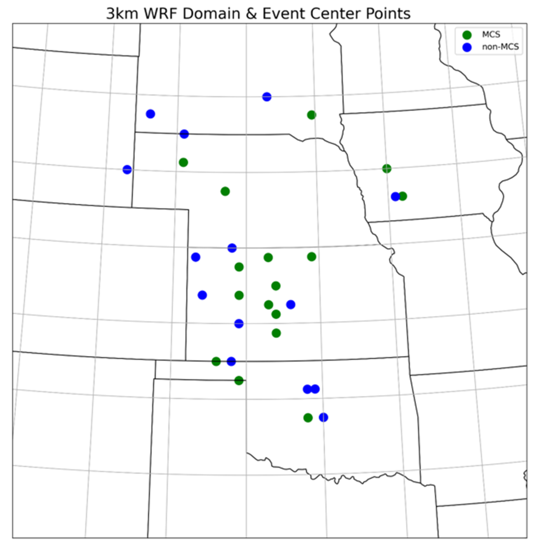
2.1. Selection of Cases

A total of 30 cases were manually selected from the months of May–August 2016. This includes 15 cases in which deep moist convection developed but did not sufficiently grow upscale to be classified as an MCS (hereafter non-MCS cases) and 15 upscale growth cases (hereafter MCS cases). Upscale growth here is defined as convection which develops initially as discrete cells and grows upscale into an MCS in an unperturbed environment. An "unperturbed" environment was defined as an environment with an absence of substantial downstream convection, as in Pinto et al. [51].
To select these events, radar data from each day were examined using the UCAR Image Archive browser (https://www2.mmm.ucar.edu/imagearchive, accessed on 3 December 2018) over the Great Plains sectors, with a focus on diurnal, not synoptically-driven, convective development and subsequent upscale growth to occur between 1600-0600 UTC. Composite reflectivity data from the lowest elevation angle of each WSR-88D radar, available at a 30 to 60-min interval, was used. Days that featured significant downstream convection and/or multiple segments with various levels of organization, or did not contain any convection, were excluded. Events that featured upscale growth outside the specified time period were also excluded.
Cases were identified based on general criteria described by James et al. [52] and Duda and Gallus [53]. An event was classified as an MCS if the convective region (contiguous reflectivity >40 dBZ) covered a sufficiently large area (100 km in length), persisted for at least two hours, and had a length:width ratio of at least 3:1. This incorporates many of the traditional morphologies, such as trailing stratiform or bow echoes, though here, the specific subtype of MCS was not identified. Non-MCS cases exhibited little if any upscale growth and did not meet the criteria described above. Additionally, a non-MCS event was required to contain at least one convective cell that persisted for at least two hours to preclude cases characterized by pulse updrafts that collapsed quickly and did not result in sustained convection.
To ensure that the general mesoscale environments were similar for the two sets of cases, both an analysis of surface boundaries and an analysis of Storm Prediction Center mesoanalysis parameters on a 40 km grid as in Mauri and Gallus [54] were performed. A front, dry line, or outflow boundary was present within 100 km of the initiating convection in 12 of the 15 non-MCS cases and in 14 of the 15 MCS cases. Using a bootstrapped t-test on 43 near-storm (averaged over the 120 × 120 km region centered on the initiation location) parameters related to winds, stability, humidity, and four composite indices as in Mauri and Gallus [54], only one near-storm parameter was significantly different between the two samples, the average relative humidity between the lifting condensation level and the level of free convection. Humidity at this level was drier in MCS cases, which might enhance evaporative cooling, possibly strengthening cold pools in those cases. Because surface features were similar along with no significant differences in almost all near-storm environmental characteristics, it is unlikely that these factors played the primary role in the results to be discussed later.

2.2. WRF Simulation Setup

The WRF-ARW version 4.0 was run using two large, coarse resolution outer domains (27-km, 9-km horizontal grid spacing) and a smaller, 3-km inner domain (Figure 1). Two-way feedback was enabled between all domains. The model domain was unchanged for all event simulations, as all 30 cases occurred within the 3-km domain. All simulations used 0.5° GFS analysis data [55] for their initial conditions and lateral boundary conditions. A total of 50 vertical layers was used, as in Squitieri and Gallus [56,57]. The Morrison double-moment microphysics scheme [58] was used for all events, as other schemes at times failed to produce realistic depictions of stratiform precipitation during testing of several MCS events (not shown, this was also observed by Thielen and Gallus [30]). For each event, the WRF was run for a total of 24 h, from 1200-1200 UTC. A full description of the model setup is found in Table 1.
In addition to the 30 simulations which used the Morrison microphysics scheme, this study also tested the impact of three other microphysics schemes on the development of convective cold pools for one MCS case (13 June 2016) and one non-MCS case (8 August 2016). For these randomly selected cases, additional WRF simulations were completed using the Thompson [59], WSM6 [60], and NSSL 2-moment schemes [61]. We compare differences of convective development and evolution, along with differences in cold pool strength, in Section 4.

2.3. Idealized CM1 Simulations

The Bryan Cloud Model (CM1, [50,62]), version 19.7, was used for idealized simulations of convection. The CM1 was run in the present study with a much higher horizontal and vertical grid spacing than the WRF (0.25-km, 98 vertical levels), allowing for investigation of the impact of storm-scale internal factors on UCG. The initial model atmosphere was horizontally homogeneous, with the base state described by an input model sounding from the WRF simulations. The base-state soundings were provided from a WRF point placed just ahead of the developing convection of interest within the unmodified near-storm environment. A basic description of the model setup is provided in Table 2.
To initialize convection in the CM1, a line of four evenly spaced warm bubbles was placed in the center of the domain. These bubbles were centered at a depth of 1.7-km, with a horizontal radius of 10-km, a vertical radius of 1.7-km, and a maximum potential temperature perturbation of 3 K. The centers of the warm bubbles were separated by a distance of 15-km. Sensitivity tests between different initialization methods (not shown) suggested that impacts to overall convective evolution did not impact whether UCG occurred, which was also implied by Parker [37] and Parker et al. [41]. In all simulations, the total time integration was 6 h. CM1 simulations used a moving domain, with the speed of the moving domain based initially on the 0–6-km mean wind vector, with additional adjustments made by trial and error to ensure the convective system remained within the domain.
In order to understand the importance of the base-state thermodynamic and kinematic profiles, four primary tests were conducted. First, a control run (hereafter CTRL) was performed by using the base-state sounding described previously. Second, isothermal layers were introduced to approximately the lowest 250 m of the input sounding (hereafter SBL250) and 750 m (SBL750). Third, the wind profiles of the MCS and non-MCS cases were interchanged (WINDR). Although modifying the base-state sounding can introduce spurious convection, reasonable results can still be obtained from a variety of thermodynamic and kinematic alterations (e.g., Adams-Selin [62,63] use 9 combinations of surface qv and 0–5-km wind shear). For all tests, a passively advected fluid tracer was initialized in the lowest 500 m of the model, with a second passive tracer added between 4–5 km. This allowed for examination of updraft and downdraft origins, respectively. Increased concentrations of the near-surface tracer within the mid to upper levels implied that surface-based air was ingested into convective updrafts, while the mid-level tracer at the bottom model layer indicated that downdrafts were capable of penetrating to the surface.

2.4. Cold Pool Parameters

To quantify the strength and structure of the 3-dimensional cold pools of MCS and non-MCS cases, several cold pool parameters were calculated, following Squitieri and Gallus [57]. The cold pool parameter (C, [33,64,65], etc.)—which represents a theoretical speed of a two-dimensional gravity current (e.g., the cold pool), perturbation potential temperature (θ′), cold pool depth, and buoyancy fields were obtained. A generalized equation of C from Weisman [32] and James et al. [66] is given by:
C 2 = 0 H ( B )   d z  
where B is buoyancy, and H is the top of the cold pool, defined here as the lower of either (a) the height where B first becomes positive or (b) the freezing level height. The constraint (b) was introduced here to ensure that only melting and evaporative processes were included. There were often times where negative values of B extended several kilometers above the freezing level height, leading to what appeared to be unrealistically high C values. Both of these methods were similar to WRF-based calculations of the cold pool by Squitieri and Gallus [57].
Buoyancy is defined as:
B g [ θ θ ¯ + 0.61 ( q v q v ¯ ) q c q r ]
In (2), g is gravity and θ   ¯ and θ′ are ambient mean potential temperature and perturbation potential temperature, respectively. Water vapor, cloud water, and rainwater mixing ratios are represented by qv, qc, and qr, where q ¯ v represents the ambient mean vapor mixing ratio.
In the CM1, calculations of the cold pool and the variables described in (2) are directly derived from the base-state condition, and C, B, and θ′ are explicitly output by the model itself. However, in WRF, the ambient environment is heterogeneous, which must be considered. The methods of Squitieri and Gallus [57] are utilized heavily for WRF calculations of the cold pool. To ensure that calculations of the cold pool parameters included only the convective areas of interest, the WRF data were subset to small (typically 4° × 3° or smaller) subdomains that were large enough to cover the entirety of the convective lifecycle from initiation to the end of the analysis period without capturing other convection not relevant to the system of interest. The ambient environment was calculated on this domain and was defined as the area where Δθ (the change in surface potential temperature between times tcurrent and t + 30 min) was negative (i.e., the area where the cold pool moves over the next 30 min). Of this area, only the bottom quartile of Δθ values was used to eliminate noise (see Squitieri and Gallus [57], their Figure 2). To evaluate possible differences in cold pools of MCS and non-MCS cases, several statistical tests were performed at each of the first five hours following convective development. The median, 75th, 90th, 95th, and 99th percentile values of each variable were calculated for each case, and these values were aggregated to evaluate differences between MCS and non-MCS events. Due to the small sample size used here, bootstrapped t-tests were employed, with a resampling of n = 1000 on both the cold pool variables C, θ′, Δθ, and cold pool depth, as well as several vertical wind shear magnitudes.

3. Results

3.1. WRF Predictability of UCG

Though the primary focus of this paper was to evaluate if there were notable differences in any cold pool variables (storm-scale, internal forcing) or bulk wind difference (BWD—an external forcing; [2]) between convective events that feature UCG and those that do not, it was first worthwhile to evaluate whether the WRF is capable of consistently predicting general evolution of convection into MCSs or non- MCSs using this specific WRF setup. To evaluate general predictability, we employ a 2 × 2 contingency table (Table 3). A WRF-simulated MCS was required to meet the same criteria defined in Section 2. Furthermore, we required WRF forecasts to simulate convective initiation within three hours of the observed CI time and within 150 km, which all of the cases did. In this study, WRF showed a high probability of detection of 0.867 (0.733) for MCS (non-MCS events). Simulated MCS events also had a higher critical success index (0.684 vs. 0.647), but a higher false alarm rate (0.235 vs. 0.154) compared to simulated non-MCS events, although false alarm rates were relatively low for both types of systems. A slight overprediction of MCS events was noted in the WRF, where 4 of the 6 total incorrect forecasts were observed non-MCS events were predicted as MCS events in the WRF (Simulated output is available online at https://meteor.geol.iastate.edu/~zhiris/WAF, acced on 25 May 2021).

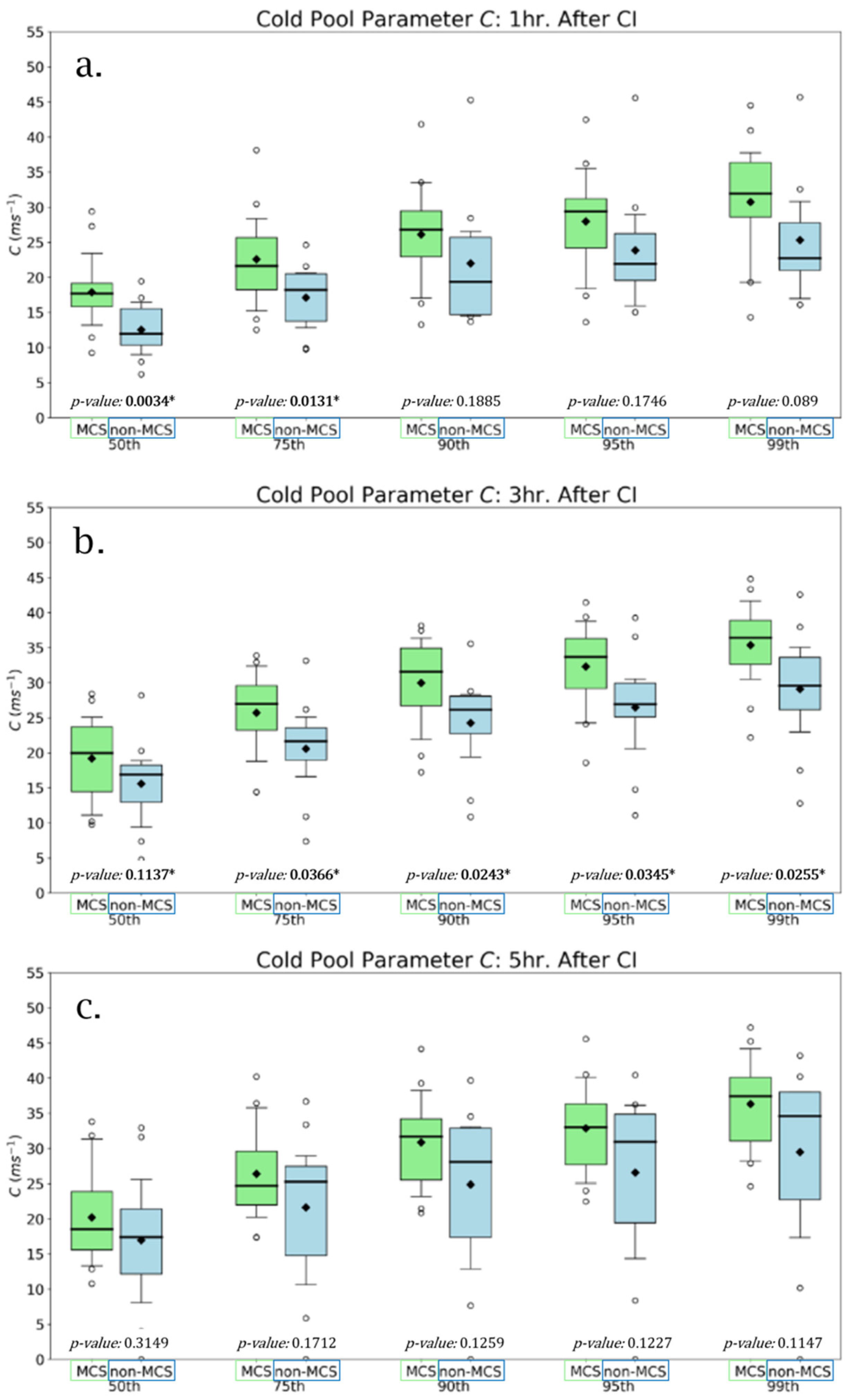
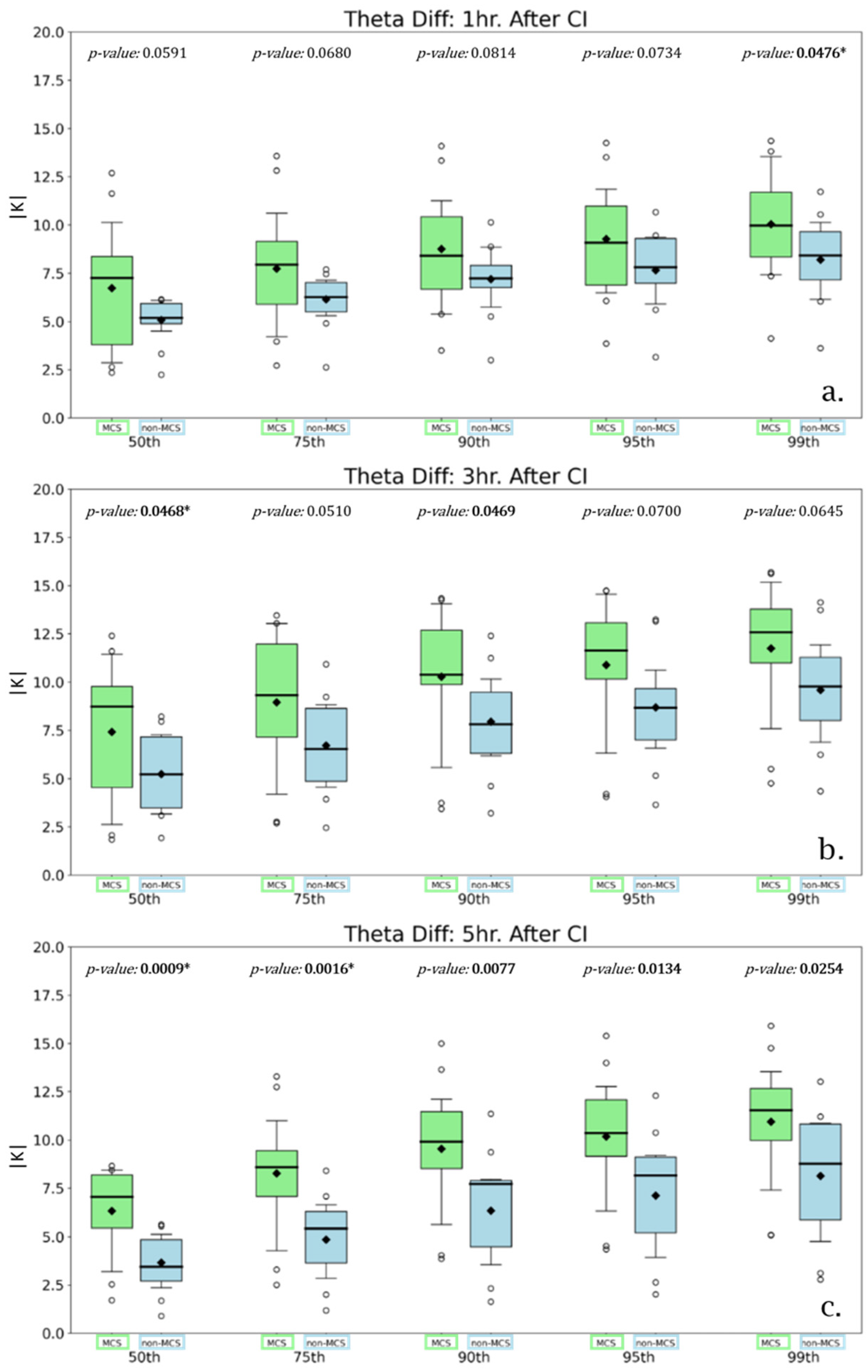
3.2. WRF Simulated Cold Pool Strength

The strength and structure of convectively generated cold pools were evaluated within the first five hours of convective initiation in all cases to investigate if cold pool strength could be correlated with UCG. We evaluated the first five hours following convective initiation to focus on the first stages of convective evolution, where UCG occurs in the MCS events, and little or no upscale growth occurs in the non-MCS cases. Identification of the first convective cells was challenging due to quickly evolving clusters of convection combined with a 30-min output time in WRF simulations, which required subjective identification of the proper convective cells at times. Cold pool variables were investigated by comparing the nth percentile value of each MCS and non-MCS event, as done by Squitieri and Gallus [57]. For all hours, the bootstrapped t-test was employed to determine if cold pools associated with developing MCSs were significantly stronger compared to those of non-MCS cases. Statistical significance was assumed if p < 0.05 [67].
In the first hour after convective initiation, the cold pool parameter C was statistically significantly larger in magnitude for MCS events at the 50th and 75th percentiles (p < 0.01, Figure 2a). The median (mean) C value for MCS cases was 17.69 (17.87) m s−1, compared to 12.52 (11.99) m s−1 in non-MCS cases, with no overlap between the interquartile range (IQR) of the MCS and non-MCS events. While there were no significant differences in the higher percentile values of C, there was still a notable difference in IQR, median, and mean values of C at each percentile used. There were statistically significant differences in C three hours after CI, particularly across the higher percentile thresholds (Figure 2b); however, statistically insignificant results (p ~ 0.1–0.2) were common during the following hours (Figure 2c).
While the comparison of the cold pool parameter C showed few significant differences in cold pool strength at most percentiles after the first hour, other cold pool variables revealed statistically significant differences in strength between MCS and non-MCS events. The perturbation potential temperature (θ′) was significantly colder in MCS cases at all percentile thresholds from one hour to three hours after convective initiation (Figure 3), with values approximately 2–3 K colder in MCS events. The statistical significance of these differences decreased over time (by hour 5, p-values are near 0.10). The potential temperature change (Δθ) only showed a statistically significant difference in the 99th percentile at hour one and 50th and 90th percentiles at hour three (Figure 4a,b). Unlike θ′, statistical significance was noted at all percentiles by hour five, and notable (p-values < 0.01) significant differences were found (Figure 4c). These results suggest that the more intense temperature gradient and colder cold pools in MCS events during the first few hours could lead to greater lift along the leading edge of the cold pools than in the non-MCS cases, facilitating UCG.
To test if cold pool distributions were affected by large, weakly negatively buoyant stratiform regions, a similar analysis was done, but only for the more pronounced convective regions (>45 dBZ) of the cold pool. When only accounting for the convective cores within the cold pool, the cold pool parameter C showed no statistical differences between MCS and non-MCS events, but Δθ remained statistically significant at hour five (not shown). Both θ′ and Δθ produced larger differences than when accounting for the entire cold pool, although differences in θ′ were still not statistically significant. Again, this result is consistent with the idea that a stronger temperature gradient at the leading edge of the cold pool would enhance lift there, making UCG more likely. The lack of significant differences in C, however, suggests that perhaps C values may be underestimating the true cold pool strength as a result of the “capping” of the depth of the cold pool described in Section 2. This formulation may underrepresent the strongest portions of the cold pool, particularly near the strongest convective cores, where negatively buoyant air can exist well above the freezing level. This is further supported by a lack of statistically significant differences between MCS and non-MCS cold pool depths (not shown). Despite some uncertainties in the importance of C in this study, the statistically significant differences in other cold pool variables suggest there are notable differences in overall cold pool strength between MCS and non-MCS events.

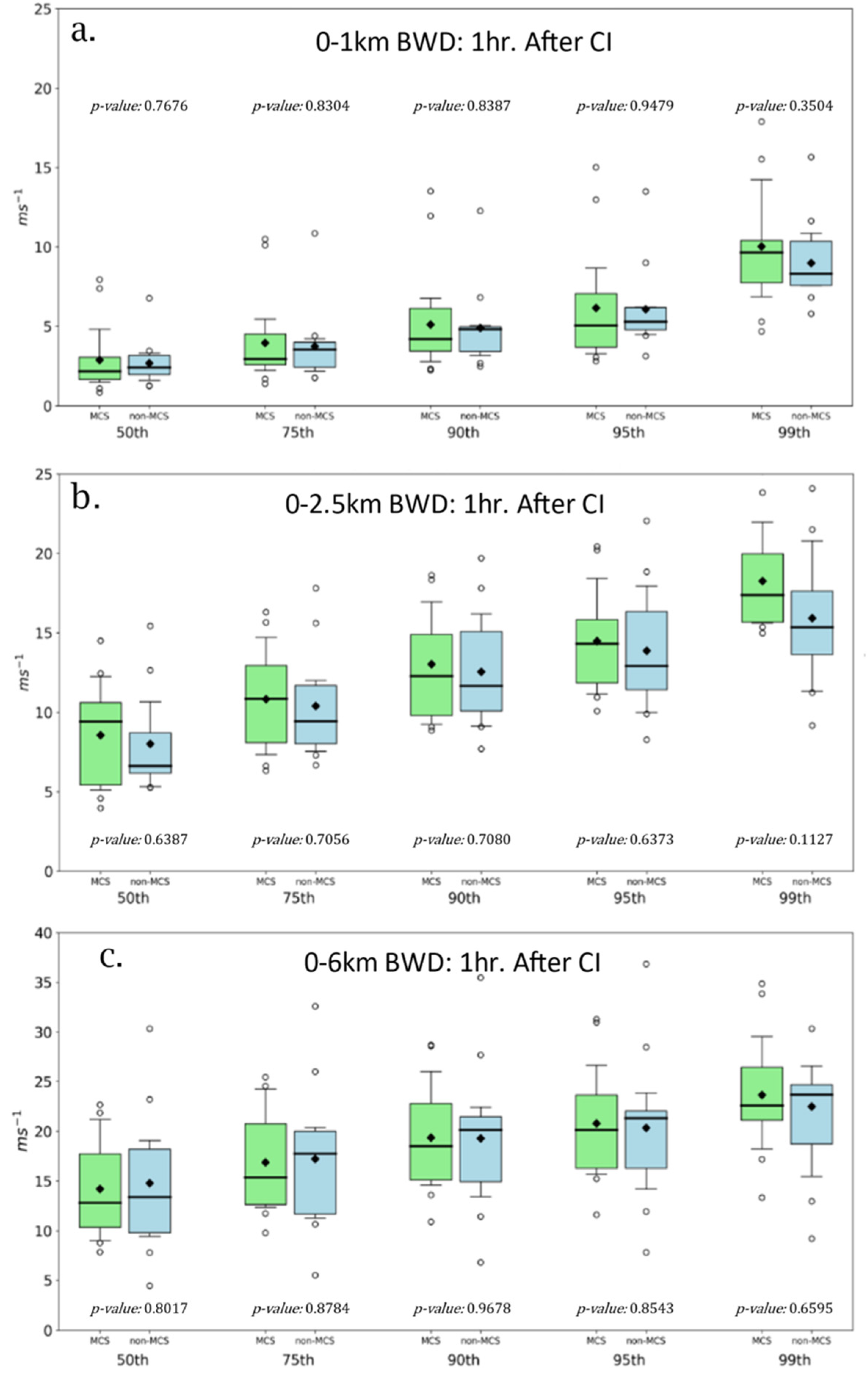
3.3. WRF Bulk Wind Difference

Low, mid, and deep layer bulk wind difference (BWD) were investigated through similar methods as described in the previous subsection. Specifically, 0–1-km, 0–2.5-km, and 0–6-km BWD were examined over the same five-hour period as the cold pool variables. BWD magnitude was found to be a poor discriminator between MCS and non-MCS events (Figure 5). Deep-layer (0–6 km) BWD magnitude differences were insignificant at all hours and percentile values, with a minimum p-value of 0.36. There was considerable overlap between the IQR of MCS and non-MCS events (e.g., Figure 5c), and median values typically differed by less than 1 m s−1. Similar results were found for 0–1-km and 0–2.5-km BWD, with no statistically significant results found (Figure 5b,c).
While it was found that BWD magnitude was not a statistically significant discriminator between MCS and non-MCS environments, it is worth reiterating that several other studies have found that wind shear and wind shear components relative to system orientation [12], combined with many other thermodynamic components [13,14] can have important implications on UCG. As stated earlier, an analysis of 43 near-storm parameters in the SPC mesoanalysis dataset did not find statistically significant differences between the MCS and non-MCS environments except for relative humidity between the LCL and LFC. In addition, a general overview suggests that nearly all MCS cases occurred in environments favorable for supercells (a Supercell Composite [68] of 2 or greater), with approximately half of the non-MCS events also occurring in supercell environments (not shown). The similarity of the near-storm parameters may explain why BWD magnitudes by themselves were a poor discriminator of non-MCS and MCS events in our sample of cases.

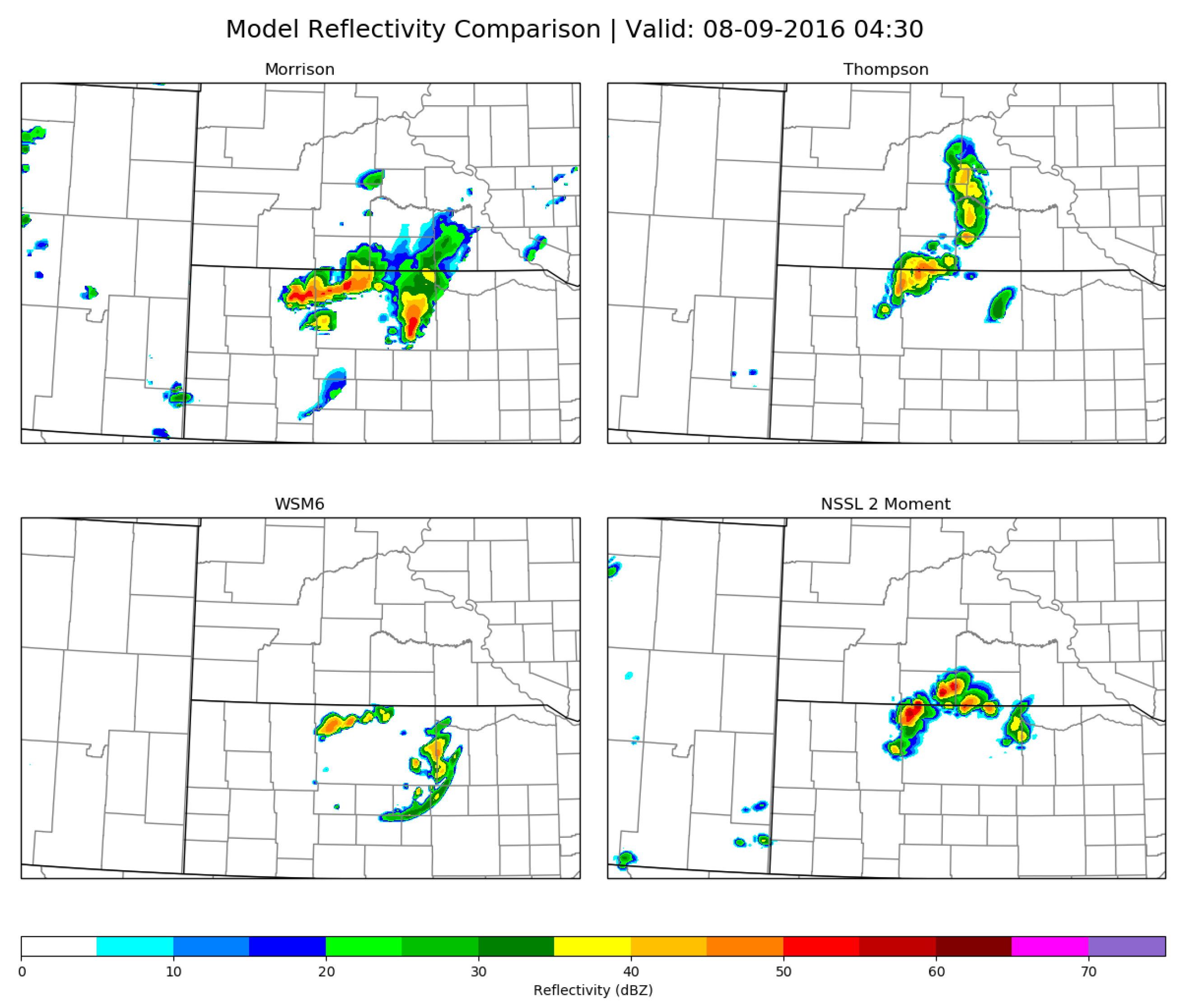
3.4. WRF UCG Sensitivity to Microphysics

In addition to the Morrison microphysics scheme used in the results discussed above, an additional 2-moment scheme (NSSL-2), a hybrid (Thompson; double moment for rain, partially double moment for graupel), and a single-moment microphysics scheme (WSM6) were also used to simulate both an MCS and a non-MCS case, chosen randomly, to test the sensitivity of UCG to variations in microphysics schemes. In both the MCS and non-MCS event, all four of the microphysics schemes tested produced similar convective evolution (discussed later). In general, the WSM6 produced the strongest cold pools of the four schemes and produced gust fronts earlier in the storm life cycle than any other scheme in both the MCS and non-MCS events. In both event types, convective initiation was not impacted substantially by microphysics choice and occurred within a 30-min window between all microphysics schemes (not shown).
In the 13 June 2016 MCS event, all four microphysics options produced generally similar convective evolution across southeastern Colorado, southwestern Kansas, and the Oklahoma and Texas Panhandles, with an MCS developing approximately five hours after convective initiation (Figure 6). Convective evolution is similar in each of the four simulations, though minor differences emerged well into the convective system lifetime, likely as a result of differences in cold pool intensity (Figure 7). The WSM6 produced a stronger and deeper cold pool than present with the other three schemes, with the other schemes all relatively similar in magnitude to one another. In the WSM6 test, median C values peaked five hours after convective initiation at just over 30 m s−1, with median θ′ magnitudes of −11 K and median cold pool depths of over 2500 m. These were larger in magnitude than in any of the other three microphysics schemes, whose median C values at peak cold pool strength ranged from 23–27 m s−1, while θ′ values never exceeded −10 K (Figure 8). The more intense cold pools in the WSM6 simulation caused the MCS to evolve through its lifecycle faster due to the stronger cold pool favoring a more rapid development of upshear tilt, and thus, the outflow boundary/gust front ran out ahead of the updraft region (and overwhelmed the horizontal vorticity from the ambient vertical shear). Other microphysics schemes did show evidence of a gust front, though it appeared later (>90 min), and there was slightly more convection generated behind the gust front compared to the WSM6. Given that other microphysics schemes all produced similar magnitudes of C, θ′, and cold pool depth, the early dissipation of convection was almost certainly related to the stronger cold pools the WSM6 generated. The idea that a cold pool could become too strong to support continued upscale growth (or eventual MCS maintenance) has been posed before, particularly from the application of RKW theory (Rotunno et al. [33]; Weisman and Rotunno [65]; James et al. [52,66]). While most studies have focused on the maintenance of a pre-existing MCS, the cold pool/shear balance described in RKW may also be applicable to the organization stages of an MCS as well.
In the 8 August 2016 non-MCS event, differences in median and mean cold pool variables were less notable (Figure 9a) among the four schemes. Despite differences in cold pool parameters, none of the microphysics schemes resulted in UCG sufficient to meet MCS criteria. Each of the four microphysics schemes at one point in time had the largest mean and median magnitude of C, which was relatively unsurprising given that cold pools are influenced by how long convection has persisted and each cells’ convective downdraft strength, and because individual cells developed/decayed differently among the four microphysics simulations (Figure 9 and Figure 10). Interestingly, there were clear differences in mean/median surface potential temperature perturbation (θ′) and cold pool depth among the schemes. The NSSL 2-moment scheme produced a deeper cold pool (generally > 200 m more) than any other scheme, which was not the case for the MCS event. The WSM6 produced the largest magnitude of θ′ at nearly all model output times, with a peak median θ′ of nearly −12 K, which was 2–3 K colder than with any other microphysics scheme (Figure 9b). There was also evidence of several gust fronts in the WSM6 simulated radar reflectivity field (Figure 10 and Figure 11) and temperature fields (not shown), suggesting that the somewhat more aggressive cold pool generation of the WSM6 compared to the other microphysics schemes led to slightly earlier storm cell dissipation.
The Morrison, Thompson, and NSSL 2-moment schemes all produced relatively similar distributions of C and θ′, and, since synoptic-scale details were similar, led to generally consistent convective evolution.

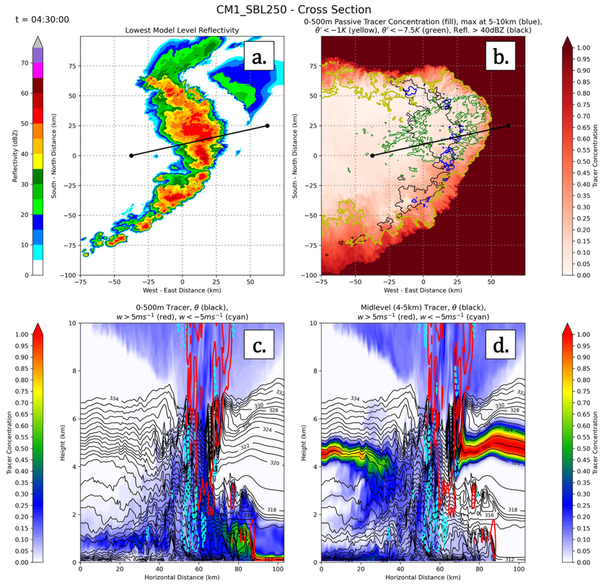
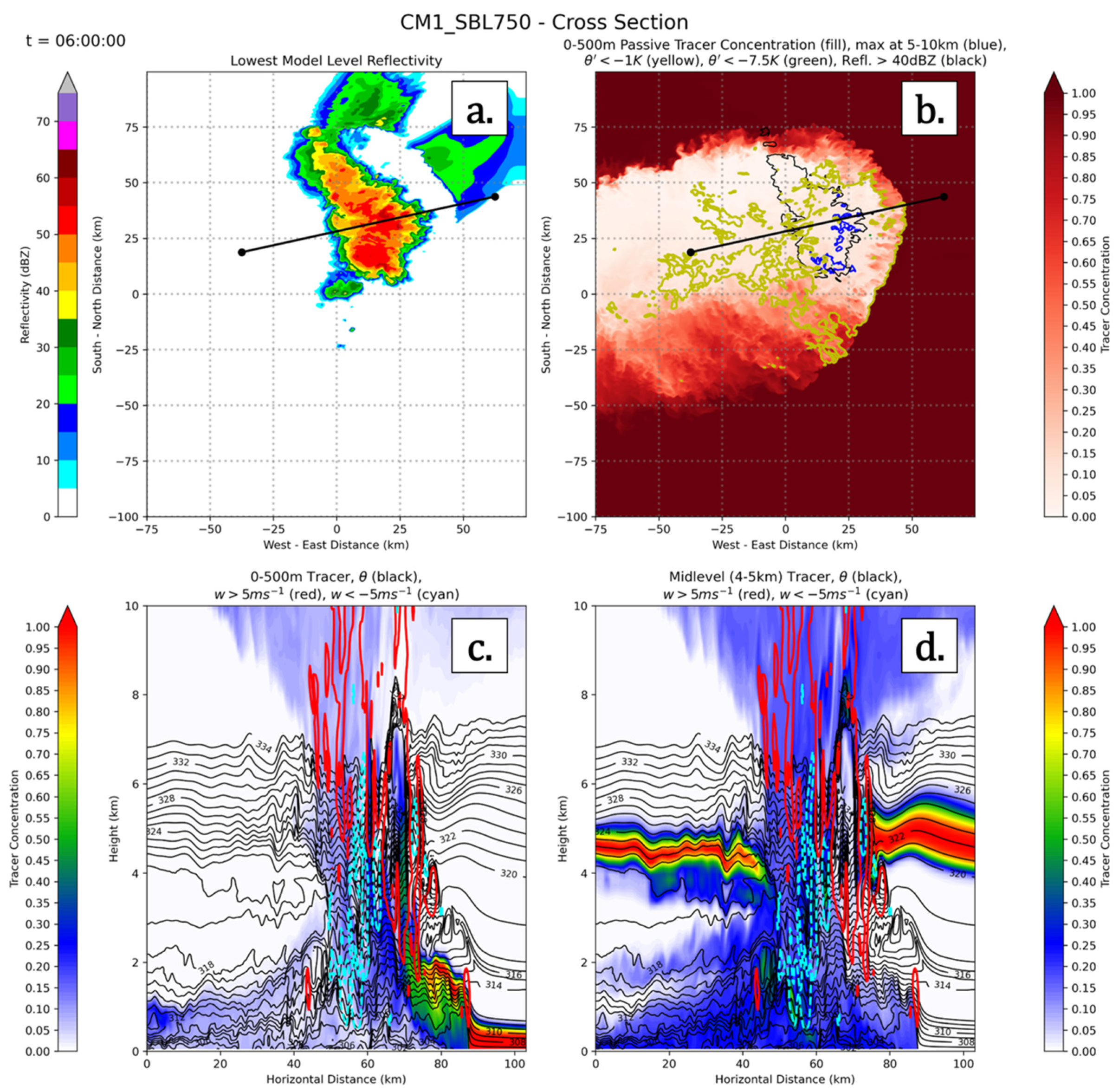
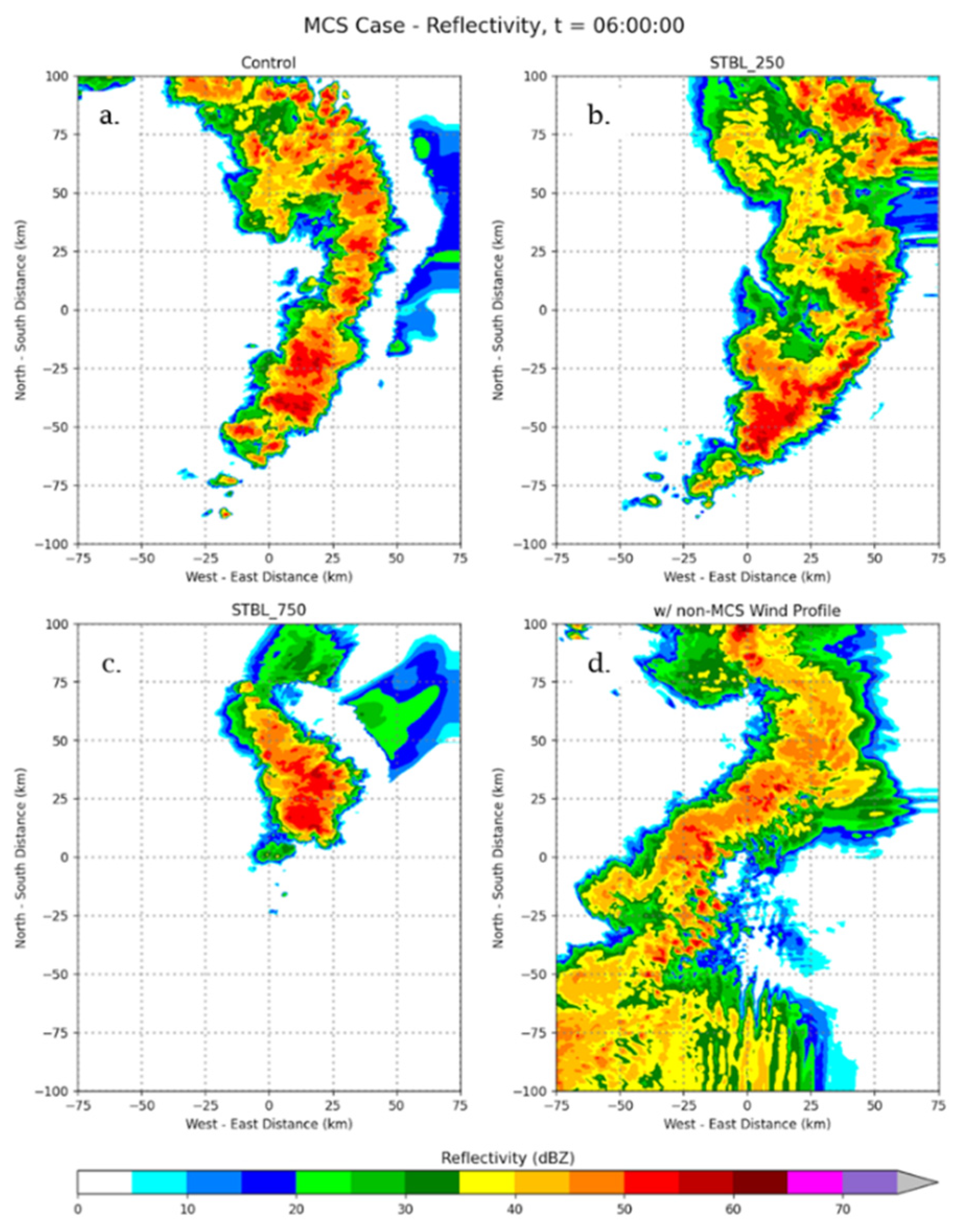
3.5. CM1 Tests of UCG

Both the 13 June 2016 MCS and 8 August 2016 non-MCS cases were simulated with the CM1 using WRF soundings (Figure 12) as input to investigate the impacts of internal factors on convective behavior. Both CTRL experiments in the CM1 were able to capture the general morphology and storm lifecycle relatively well. In the simulated MCS case, a large bowing MCS formed within five hours of convective initiation. Though there are differences in storm-scale features compared to both the WRF simulation and observations, the convective structure was similar (Figure 13). The CTRL sounding (Figure 12a) was favorable for surface-based convection. The CM1 updrafts contained 0–500-m tracer through the duration of the simulation, and a strong cold pool developed early in the simulations (Figure 14). However, cross-section analysis suggested that a surface-based lifting mechanism (i.e., the cold pool leading edge) was not entirely responsible for lifting ambient air into the system’s updraft. The system was very clearly outflow (cold pool) dominant, with the leading edge of the cold pool displaced by up to 25 km ahead of the leading edge of convection across portions of the line (Figure 14d). Additionally, there was evidence of gravity wave-like structures between 2–4 km, and surface-based tracer concentrations through this layer exhibit a wave-like appearance aloft, coincident with areas of higher vertical velocity (Figure 14a). It is at least possible that the combination of the surface-based cold pool and subsequent lift on the cold pool edge, combined with lift from the gravity-wave-like structures, both contributed to the generation of new convective updrafts.
In the 250-m deep stable layer (SBL250) experiment, the convection still grew up-scale into an MCS, and MCS progression was generally similar to the CTRL simulation (Figure 15). Despite surface temperatures initially on the order of ~3 K lower than in CTRL, the SBL250 experiment still developed a surface-based cold pool within an hour of convective initiation. In the deeper, isothermal environment in the 750-m deep stable layer (SBL750) simulation, UCG still occurred, albeit at a slower rate than the CTRL and SBL250 MCS simulations (Figure 16). The initial four cells congealed into a single cell quickly and gradually grew into a smaller convective system that almost but does not quite meet the size requirements for an MCS. Initially, surface potential temperature perturbations were positive, but a cold pool still formed midway through the 6-hr simulation. When the cold pool formed, surface-layer tracers were contained in the updraft, indicating that surface or near-surface-based convection occurred in the presence of an initially deep surface-based stable layer (Figure 16a). In both stable boundary layer simulations, evidence again suggested that the cold pool edge is not solely responsible for convective updraft generation. As in the CTRL experiment, wave-like patterns in surface tracer concentrations were evident and were particularly notable in the SBL250 experiment (Figure 15a).
In the MCS WINDR experiment (Figure 17), despite the use of the non-MCS wind profile, extensive convective development still occurred and was sustained through the duration of the simulation, which is generally consistent with the WRF analysis, which showed that wind shear magnitude did not discriminate well between MCS and non-MCS events. There was far more extraneous, weaker convection on the southern flank of the WINDR-produced system compared to that of the observed MCS and the CTRL, SBL250, and SBL750 experiments. However, an MCS still developed, and some of the reflectivity characteristics were at least broadly comparable to both the simulated CTRL and observed reflectivity from the event (in particular, there is still evidence of some sort of bowing MCS shown in Figure 17). This result is somewhat consistent with what was found from the analysis of the WRF run and supports the assertion that BWD magnitude by itself may not exert a controlling influence on upscale convective growth.
The sounding used to initialize the non-MCS case has a deeper and drier PBL but also less steep lapse rates above the LFC compared to the MCS case (Figure 12). These environmental differences likely impact the degree of convective organization, although it is difficult to isolate the impacts of each difference. The drier and deeper PBL could support a stronger cold pool, but the less steep lapse rates aloft would favor weaker updrafts and less production of condensate, especially since mixing ratios at the LFC are much lower in the non-MCS case than in the MCS case. In addition, the weaker buoyancy in the non-MCS case with relatively “skinny” CAPE would make the convection in that case more susceptible to weakening or dissipation due to dry air entrainment. The non-MCS CTRL case sustained one cell for just under four hours before dissipating. This was generally a shorter storm lifecycle compared to what was both observed and simulated in the WRF (not shown). The CTRL CM1 was similarly unable to sustain convection and generate upscale growth, despite a favorable thermodynamic profile and essentially no convective inhibition in the base-state sounding. Convection was sustained longer in the non-MCS SBL250 experiment compared to CTRL, with a single cell sustained for the entire duration of the simulation (Figure 18a,b). The SBL750 experiment was relatively similar to the CTRL, in which convective cells dissipated within a few hours of the simulation, though the SBL750 cell persisted for less time than the CTRL (Figure 18c). In the WINDR experiment, convection failed to be sustained through the duration of the simulation and dissipated more rapidly than in any other CM1 non-MCS simulation (Figure 18d). It is unclear why only the SBL250 simulation maintained convection throughout the duration of the simulation. Broad cold pools develop in each of the simulations (not shown), and among the CM1 MCS and non-MCS experiments, differences in CAPE and CIN were small (<10 J kg−1 and <2.5 J kg−1, respectively), which suggests that even subtle thermodynamic changes may have potentially large impacts on convective evolution.

4. Discussion and Conclusions

This work provides a characterization of model-simulated 3-D cold pools across a number of both MCS and non-MCS warm-season convective events in the northern and central Great Plains. While previous studies have focused on single events (e.g., [39]) and cold pools at MCS maturity (e.g., [56]), the authors are unaware of any studies which investigate a few near-storm and storm-scale parameters thought to influence the upscale growth potential of deep moist convection utilizing both convection-allowing WRF experiments and cloud-resolving CM1 experiments. To accomplish this, a total of 15 MCS and 15 non-MCS convective events from the 2016 warm season were simulated using WRF.
From the WRF simulations performed, it was shown that surface-based cold pool variables (e.g., Δθ and θ′) are larger in magnitude in MCS events compared to in non-MCS events. In particular, perturbation potential temperature (θ′) showed a strong statistical significance within the first few hours, where θ′ values in MCS events were 2–3 K colder than in non-MCS events. Conversely, magnitudes of Δθ were significantly larger in MCS events from hours two through five, with near statistical significance observed in the first hour (p ~ 0.07) and strong significance in the last hour (p < 0.01). When accounting for only the actively convective (dBZ > 45) areas of the cold pool, the differences in these variables are equally or slightly more statistically significant compared to the entire cold pool region.
Interestingly, the cold pool parameter C, which is an integration of the total negative buoyancy in the column, showed less ability to differentiate between MCS and non-MCS events. It is possible that this result is related to our constraint on the depth of the cold pool to not exceed the freezing level. Future work should compare magnitudes of C from a larger sample of idealized experiments, where C is substantially easier to calculate, which could provide more valuable insight into its importance.
BWD magnitude in isolation was also found to have little effect on the convective evolution of events in this study, with statistically insignificant results found using the 0–1-, 0–2.5-, and 0–6-km layers. The present study did not consider the line-normal vs. line-parallel shear vector components, as many non-MCS events in this study produced greatly varying storm motions (at times, storm motion of individual cells varied by more than 45 degrees). Results here suggest that BWD magnitudes themselves are a poor discriminator of events, given the wide overlap between MCS and non-MCS environments.
To determine the impacts of the specific cloud microphysics parameterization schemes used in the WRF, the cold pools produced by three other microphysics schemes (WSM6, NSSL2, Thompson) were compared with those from the Morrison scheme used as a control. These schemes were tested on one randomly chosen MCS event and one non-MCS event. Generally, each of the four microphysics schemes produced similar convective patterns during the upscale growth phase of convective development. The WSM6 microphysics scheme produced the strongest cold pool in the MCS event, with C and θ′ magnitudes approximately 5 m s−1 and 1 K greater, respectively, than the values from the other schemes. The WSM6 also produced an apparent gust front evident in the lowest model reflectivity before any other scheme and diminished convection quicker as a result. In the non-MCS event, there were no clear differences between the microphysics schemes in peak magnitudes of C, but the WSM6 again had greater magnitudes of θ′, up to 2–3 K cooler than with any other scheme. Each produced cellular convection that failed to grow sufficiently upscale to meet MCS criteria, which suggests that upscale growth may not be strongly dependent on the choice of microphysics scheme, at least in this case. However, it should be noted that these tests were performed on only one case and did not consider specific MCS subclasses. Thielen and Gallus [30] did show some dependence of upscale growth on the microphysics scheme used in a larger sample of 10 cases.
Finally, in addition to the analysis of the 30 WRF simulations to examine upscale growth, thermodynamic and kinematic sensitivities were tested in several CM1 experiments. Using WRF sounding data for initialization, the CTRL runs of both an MCS and a non-MCS event produced appropriate representations of convective mode (e.g., MCS or non-MCS). This also occurred when a shallow stable layer (SBL250 experiments) was introduced, and to some extent, when a deeper stable layer (SBL750 experiments) was used. In all of the MCS experiments, a surface cold pool developed and spread laterally. This is consistent with results from observational studies [48] and recent work with CM1 in stable boundary layers [41].
Lastly, switching the wind profiles of the MCS and non-MCS event did not significantly change the overall convective evolution in the CM1. This supports the findings from the WRF-based portion of this study, which suggest that overall convective evolution is primarily driven by the near-storm thermodynamic environment, and in particular, how it affects cold pool intensity. When the non-MCS case wind profile was used with the MCS case temperature and dewpoint profiles, many of the convective system characteristics were maintained—a weakly bowing, cold pool dominant MCS grew upscale at a similar rate as in the control and stable boundary layer CM1 experiments. Additionally, the non-MCS thermodynamic profile combined with the MCS wind profile produced brief, cellular convection, which further supports this argument.
The upscale convective growth phase of deep moist convection remains poorly understood and forecast (e.g., [29,39]) and represents an area of significant interest for operational forecasts of severe convection (e.g., [2,7,18]). Results from this study show that convectively generated cold pools leading to upscale growth into MCSs in the WRF are significantly stronger—particularly at the surface (via θ′ or Δθ)—during the first several hours following convective initiation. However, differences in vertical wind shear magnitudes were found to be insignificant across all statistical tests performed in this study. This suggests that the primary mechanism for upscale growth into larger, more organized convective systems is through the generation of a cold pool itself, rather than synoptic-scale kinematic fields, especially in regimes with weak synoptic forcing.
It is recommended that future work incorporate both WRF and CM1 in tandem, as done in the present study, to better discern what causes upscale growth into MCSs in heterogeneous and homogeneous environments. In particular, the internal drivers of MCSs should be investigated in more detail to improve the understanding of MCSs in both surface-based and elevated convective regimes. The authors here advise investigating the importance of the mid-level temperature and moisture and/or the low- to mid-level θe profile in its relation to both cold pool generation subsequent upscale convective growth into MCSs. Future work should also look to investigate the importance of line-normal vs. line parallel shear vectors in tandem with the cold pool.

Author Contributions

Conceptualization, Z.A.H. and W.A.G.J.; methodology, Z.A.H. and W.A.G.J.; software, Z.A.H.; validation, Z.A.H. and W.A.G.J.; formal analysis, Z.A.H.; investigation, Z.A.H.; resources, W.A.G.J.; data curation, Z.A.H.; writing—original draft preparation, Z.A.H.; writing—review and editing, Z.A.H. and W.A.G.J.; visualization, Z.A.H.; supervision W.A.G.J.; project administration, W.A.G.J.; funding acquisition, W.A.G.J. All authors have read and agreed to the published version of the manuscript.

Funding

This work was funded by NSF Awards AGS16249 and AGS2022888.

Institutional Review Board Statement

Not Applicable.

Informed Consent Statement

Not Applicable.

Data Availability Statement

All archived GFS analyses data used in this study are openly available through the NOAA/NCEI NOMADS model data archive (see reference NOAA/NCEI 2019). Due to its storage size, all WRF and CM1 simulations are archived locally at Iowa State and are not publicly accessible but are available upon request by contacting the corresponding author.

Acknowledgments

The authors would like to thank Jon Thielen for his extensive help in providing Python code used during various portions of this work and Brian Squitieri for the original code used for calculating the cold pool parameters. Anna Duhachek is thanked for performing the analysis of synoptic fronts and near-storm parameters. The authors extend thanks to Dave Flory and Daryl Herzmann of Iowa State for their help in assisting with the Iowa State supercomputers, which were used extensively over the course of this work. The constructive comments of two anonymous reviewers helped to improve the paper substantially.

Conflicts of Interest

The authors declare no conflict of interest. The funders had no role in the design of the study; in the collection, analyses, or interpretation of data; in the writing of the manuscript, or in the decision to publish the results.

References

  1. Blanchard, D.O. Mesoscale convective patterns of the Southern High Plains. Bull. Am. Meteor. Soc. 1990, 71, 994–1005. [Google Scholar] [CrossRef] [Green Version]
  2. Thompson, R.L.; Edwards, R.; Hart, J.A.; Elmore, K.L.; Markowski, P. Close proximity soundings within supercell environments obtained from the Rapid Update Cycle. Weather Forecast. 2003, 18, 1243–1261. [Google Scholar] [CrossRef] [Green Version]
  3. Doswell, C.A.; Brooks, H.E.; Kay, M.P. Climatological estimates of daily nontornadic severe thunderstorm probability for the United States. Weather Forecast. 2005, 20, 577–595. [Google Scholar] [CrossRef] [Green Version]
  4. Gallus, W.A., Jr.; Snook, N.A.; Johnson, E.V. Spring and summer severe weather reports over the Midwest as a function of convective mode: A preliminary study. Weather Forecast. 2008, 23, 101–113. [Google Scholar] [CrossRef] [Green Version]
  5. Smith, B.T.; Thompson, R.L.; Grams, J.S.; Broyles, C.; Brooks, H.E. Convective modes for significant severe thunderstorms in the contiguous United States. Part I: Storm classification and climatology. Weather Forecast. 2012, 27, 1114–1135. [Google Scholar] [CrossRef] [Green Version]
  6. Thompson, R.L.; Smith, B.T.; Grams, J.S.; Dean, A.R.; Broyles, C. Convective modes for significant severe thunderstorms in the contiguous United States. Part II: Supercell and QLCS tornado environments. Weather Forecast. 2012, 18, 1243–1261. [Google Scholar] [CrossRef] [Green Version]
  7. Nielsen, E.R.; Herman, G.R.; Tournay, R.C.; Peters, J.M.; Schumacher, R.S. Double impact: When both tornadoes and flash floods threaten the same place at the same time. Weather Forecast. 2015, 30, 1673–1693. [Google Scholar] [CrossRef]
  8. Clark, A.J.; Gallus, W.A., Jr.; Xue, M.; Kong, F. A comparison of precipitation forecast skill between small convection-allowing and large convection-parameterizing ensembles. Weather Forecast. 2009, 24, 1121–1140. [Google Scholar] [CrossRef] [Green Version]
  9. Schwartz, C.S.; Kain, J.S.; Weiss, S.J.; Xue, M.; Bright, D.R.; Kong, F.; Thomas, K.V.; Levit, J.J.; Coniglio, M.C. Next-day convection-allowing WRF model guidance: A second look at 2-km versus 4-km grid spacing. Mon. Weather Rev. 2009, 137, 3351–3372. [Google Scholar] [CrossRef]
  10. Kain, J.S.; Coniglio, M.C.; Correia, J.; Clark, A.J.; Marsh, P.T.; Ziegler, C.; Lakshmanan, V.; Miller, S.D., Jr.; Dembek, S.R.; Weiss, S.J.; et al. LA feasibility study for probabilistic convection initiation forecasts based on explicit numerical guidance. Bull. Am. Meteor. Soc. 2013, 94, 1213–1225. [Google Scholar] [CrossRef] [Green Version]
  11. Jirak, I.L.; Cotton, W.R. Observational analysis of the predictability of mesoscale convective systems. Weather Forecast. 2007, 22, 813–838. [Google Scholar] [CrossRef]
  12. Cohen, A.E.; Coniglio, M.C.; Corfidi, S.F.; Corfidi, S.J. Discrimination of mesoscale convective system environments using sounding observations. Weather Forecast. 2007, 22, 1045–1062. [Google Scholar] [CrossRef] [Green Version]
  13. Coniglio, M.C.; Hwang, Y.; Stensrud, D.J. Environmental factors in the upscale growth and longevity of MCSs derived from Rapid Update Cycle analyses. Mon. Weather Rev. 2010, 138, 3514–3539. [Google Scholar] [CrossRef]
  14. Coniglio, M.C.; Corfidi, S.F.; Kain, J.S. Environment and early evolution of the 8 May 2009 derecho-producing convective system. Mon. Weather Rev. 2011, 139, 1083–1102. [Google Scholar] [CrossRef] [Green Version]
  15. Dial, G.L.; Racy, J.P.; Thompson, R.L.J. Short-term convective mode evolution along synoptic boundaries. Weather Forecast. 2010, 25, 1430–1446. [Google Scholar] [CrossRef] [Green Version]
  16. Bluestein, H.B.; Jain, M.H. Formation of mesoscale lines of precipitation: Severe squall lines in Oklahoma during the spring. J. Atmos. Sci. 1985, 42, 1711–1732. [Google Scholar] [CrossRef]
  17. Bluestein, H.B.; Marx, G.T.; Jain, M.H. Formation of mesoscale lines of precipitation: Nonsevere squall lines in Oklahoma during the spring. Mon. Weather Rev. 1987, 115, 2719–2727. [Google Scholar] [CrossRef] [Green Version]
  18. Duda, J.D.; Gallus, W.A., Jr. The impact of large-scale forcing on skill of simulated convective initiation and upscale evolution with convection-allowing grid spacings in the WRF. Weather Forecast. 2013, 28, 994–1018. [Google Scholar] [CrossRef] [Green Version]
  19. Peters, J.M.; Schumacher, R.S. The simulated structure and evolution of a quasi-idealized warm-season convective system with a training convective line. J. Atmos. Sci. 2015, 72, 1987–2010. [Google Scholar] [CrossRef]
  20. Weisman, M.L.; Skamarock, W.C.; Klemp, J.B. The resolution dependence of explicitly modeled convective systems. Mon. Weather Rev. 1997, 125, 527–548. [Google Scholar] [CrossRef]
  21. Fowle, M.A.; Roebber, P.J. Short-range (0–48h) numerical prediction of convective occurrence, mode, and location. Weather Forecast. 2003, 18, 782–794. [Google Scholar] [CrossRef]
  22. Done, J.; Davis, C.A.; Weisman, M. The next generation of NWP: Explicit forecasts of convection using the weather research and forecasting (WRF) model. Atmos. Sci. Lett. 2004, 5, 110–117. [Google Scholar] [CrossRef]
  23. Weisman, M.L.; Davis, C.; Wang, W.; Manning, K.W.; Klemp, J.B. Experiences with 0-36-h explicit convective forecasts with the WRF-ARW model. Weather Forecast. 2008, 23, 407–437. [Google Scholar] [CrossRef]
  24. Weiss, S.J.; Pyle, M.E.; Janjic, Z.; Bright, D.R.; DiMego, G.J. The Operational High Resolution Window WRF Model Runs at NCEP: Advantages of Multiple Model Runs for Severe Convective Weather Forecasting. In Proceedings of the 24th Conference on Severe Local Storms, Savannah, GA, USA, 27–31 October 2008; American Meteorological Society: Boston, MA, USA, 2008. Available online: https://ams.confex.com/ams/pdfpapers/142192.pdf (accessed on 22 February 2019).
  25. Clark, A.J.; Kain, J.S.; Marsh, P.T.; Correia, J.; Xue, M.; Kong, F. Forecasting tornado pathlengths using a three-dimensional object identification algorithm applied to convection-allowing forecasts. Weather Forecast. 2012, 27, 1090–1113. [Google Scholar] [CrossRef]
  26. Guyer, J.L.; Jirak, I.L. The utility of storm-scale ensemble forecasts of cool season severe weather events from the SPC perspective. In Proceedings of the 27th Conference on Severe Local Storms, Madison, WI, USA, 3–7 November 2008; American Meteorological Society: Boston, MA, USA, 2014. Available online: https://ams.confex.com/ams/27SLS/webprogram/Paper254640.html (accessed on 9 July 2019).
  27. Gallo, B.T.; Clark, A.J.; Jirak, I.; Kain, J.S.; Weiss, S.J.; Coniglio, M.; Knopfmeier, K.; Correia, J., Jr.; Melick, C.J.; Karstens, C.D.; et al. Breaking new ground in severe weather prediction: The 2015 NOAA/Hazardous Weather Testbed Spring Forecasting Experiment. Weather Forecast. 2017, 32, 1541–1568. [Google Scholar] [CrossRef]
  28. Hawblitzel, D.P.; Zhang, F.; Meng, Z.; Davis, C.A. Probabilistic evaluation of the dynamics and predictability of the mesoscale convective vortex of 10–13 June 2003. Mon. Weather Rev. 2007, 135, 1544–1563. [Google Scholar] [CrossRef] [Green Version]
  29. Schumacher, R.S. Resolution dependence of initiation and upscale growth of deep convection in convection-allowing forecasts of the 31 May–1 June 2013 supercell and MCS. Mon. Weather Rev. 2015, 143, 4331–4354. [Google Scholar] [CrossRef]
  30. Thielen, J.E.; Gallus, W.A., Jr. Influences of horizontal grid spacing and microphysics on WRF forecasts of convective morphology evolution for nocturnal MCSs in weakly forced environments. Weather Forecast. 2019, 34, 1495–1517. [Google Scholar] [CrossRef]
  31. Droegemeier, K.K.; Wilhelmson, R.B. Three-dimensional numerical modeling of convection produced by interacting thunderstorm outflows. Part II: Variations in vertical wind shear. J. Atmos. Sci. 1985, 42. [Google Scholar] [CrossRef]
  32. Weisman, M.L. The role of convectively generated rear-inflow jets in the evolution of long-lived mesoconvective systems. J. Atmos. Sci. 1992, 49, 1826–1847. [Google Scholar] [CrossRef] [Green Version]
  33. Rotunno, R.J.; Klemp, J.B.; Weisman, M.L. A theory for strong, long-lived squall lines. J. Atmos. Sci. 1988, 45, 463–485. [Google Scholar] [CrossRef] [Green Version]
  34. Corfidi, S.F. Cold pools and MCS propagation: Forecasting the motion of downwind-developing MCSs. Weather Forecast. 2003, 18, 997–1017. [Google Scholar] [CrossRef]
  35. McAnelly, R.L.; Nachamkin, J.E.; Cotton, W.R.; Nicholls, M.E. Upscale evolution of MCSs: Doppler radar analysis and analytical investigation. Mon. Weather Rev. 1997, 125, 1083–1110. [Google Scholar] [CrossRef]
  36. Bryan, G.H.; Rotunno, R. The optimal state for gravity currents in shear. J. Atmos. Sci. 2014, 71, 448–468. [Google Scholar] [CrossRef]
  37. Parker, M.D. External vs. Self-Organization of Nocturnal MCSs from PECAN. In Proceedings of the 29th Conference on Severe Local Storms, Stowe, VT, USA, 22–26 October 2018; American Meteorological Society: Boston, MA, USA, 2018. Available online: https://ams.confex.com/ams/29SLS/meetingapp.cgi/Paper/348312 (accessed on 9 July 2019).
  38. Peters, J.M.; Schumacher, R.S. Dynamics governing a simulated mesoscale convective system with a training convective line. J. Atmos. Sci. 2016, 73, 2643–2664. [Google Scholar] [CrossRef]
  39. Mulholland, J.P.; Nesbitt, S.W.; Trapp, R.J. A case study of terrain influences on upscale convective growth of a supercell. Mon. Weather Rev. 2019, 147, 4305–4324. [Google Scholar] [CrossRef]
  40. Parker, M.D. Self-organization and maintenance of simulated nocturnal convective systems from PECAN. Mon. Weather Rev. 2021, 149, 999–1022. [Google Scholar] [CrossRef]
  41. Parker, M.D.; Borchardt, B.S.; Miller, R.L.; Ziegler, C.L. Simulated evolution and severe wind production by the 25–26 June 2015 nocturnal MCS from PECAN. Mon. Weather Rev. 2020, 148, 183–209. [Google Scholar] [CrossRef]
  42. Marion, G.R.; Trapp, R.J. The dynamical coupling of convective updrafts, downdrafts, and cold pools in simulated supercell thunderstorms. J. Geophys. Res. Atmos. 2019, 124, 664–683. [Google Scholar] [CrossRef]
  43. Adams-Selin, R.D.; van den Heever, S.C.; Johnson, R.H. Sensitivity of bow-echo simulation to microphysical parameterizations. Weather Forecast. 2013, 28, 1188–1209. [Google Scholar] [CrossRef]
  44. Mallison, H.M.; Lasher-Trapp, S.G. An investigation of hydrometeor latent cooling upon convective cold pool formation, sustainment, and properties. Mon. Weather Rev. 2019, 147, 3205–3222. [Google Scholar] [CrossRef]
  45. Borque, P.S.; Nesbitt, W.; Trapp, R.J.; Lasher-Trapp, S.G.; Oue, M. Observational study of the thermodynamics and morphological characteristics of a midlatitude continental cold pool event. Mon. Weather Rev. 2020, 148, 719–737. [Google Scholar] [CrossRef]
  46. Peters, J.M.; Eure, K.C.; Schumacher, R.S. Factors that Drive MCS Growth from Supercells. In Proceedings of the 17th Conference on Mesoscale Processes, San Diego, CA, USA, 24–27 July 2017; American Meteorological Society: Boston, MA, USA, 2017. Available online: https://ams.confex.com/ams/17MESO/webprogram/Paper320248.html (accessed on 9 July 2019).
  47. Geerts, B.; Parsons, D.; Ziegler, C.L.; Weckwerth, T.M.; Biggerstaff, M.I.; Clark, R.D.; Coniglio, M.C.; Demoz, B.B.; Ferrare, R.A.; Gallus, W.A., Jr.; et al. The 2015 Plains Elevated Convection at Night field project. Bull. Am. Meteor. Soc. 2017, 98, 767–786. [Google Scholar] [CrossRef]
  48. Hitchcock, S.M.; Schumacher, R.S.; Herman, G.R.; Coniglio, M.C.; Parker, M.D.; Ziegler, C.L. Evolution of pre- and postconvective environmental profiles from mesoscale convective systems during PECAN. Mon. Weather Rev. 2019, 147, 2329–2354. [Google Scholar] [CrossRef]
  49. Skamarock, W.C.; Klemp, J.B.; Dudhia, J.; Gill, D.O.; Barker, D.M.; Wang, W.; Powers, J.G. A Description of the Advanced Research WRF Version 4; NCAR Technical Notes. NCAR/TN-556+STR2019; UCAR: Boulder, CO, USA, 2021; 145p. [Google Scholar] [CrossRef]
  50. Bryan, G.H.; Fritsch, J.M. A benchmark simulation for moist nonhydrostatic numerical models. Mon. Weather Rev. 2002, 130, 2917–2928. [Google Scholar] [CrossRef]
  51. Pinto, J.O.; Grim, J.A.; Steiner, M. Assessment of the high-resolution Rapid Refresh model’s ability to predict mesoscale convective systems using object-based evaluation. Weather Forecast. 2015, 30, 892–913. [Google Scholar] [CrossRef]
  52. James, R.P.; Markowski, P.M.; Fritsch, J.M. Bow echo sensitivity to ambient moisture and cold pool strength. Mon. Weather Rev. 2006, 134, 950–964. [Google Scholar] [CrossRef] [Green Version]
  53. Duda, J.D.; Gallus, W.A., Jr. Spring and summer Midwestern severe weather reports in supercells compared to other morphologies. Weather Forecast. 2010, 25, 190–206. [Google Scholar] [CrossRef] [Green Version]
  54. Mauri, E.L.; Gallus, W.A., Jr. Differences between Severe and Non-Severe Warm-Season Nocturnal Bow Echo Environments. Weather Forecast. 2021, 36, 53–74. [Google Scholar] [CrossRef]
  55. NOAA/NCEI. NCEP Numerical Weather Prediction Models Global Forecast System (GFS) Grid 004. Subset Used: May–June 2016. Available online: https://nomads.ncdc.noaa.gov/data/gfsanl/ (accessed on 1 August 2019).
  56. Squitieri, B.J.; Gallus, W.A., Jr. WRF forecasts of Great Plains nocturnal low-level jet-driven MCSs. Part I: Correlation between low-level jet forecast accuracy and MCS precipitation forecast skill. Weather Forecast. 2016, 31, 1301–1323. [Google Scholar] [CrossRef]
  57. Squitieri, B.J.; Gallus, W.A., Jr. On the forecast sensitivity of MCS cold pools and related features to horizontal grid spacing in convection-allowing WRF simulations. Weather Forecast. 2020, 35, 325–346. [Google Scholar] [CrossRef]
  58. Morrison, H.; Thompson, G.; Tatarskii, V. Impact of cloud microphysics on the development of trailing stratiform in a simulated squall line: Comparison of one- and two-moment schemes. Mon. Weather Rev. 2009, 137, 991–1007. [Google Scholar] [CrossRef] [Green Version]
  59. Thompson, G.; Field, P.R.; Rasmussen, R.M.; Hall, W.D. Explicit forecasts of winter precipitation using an improved bulk microphysics scheme. Part II: Implementation of a new snow parameterization. Mon. Weather Rev. 2008, 136, 5095–5115. [Google Scholar] [CrossRef]
  60. Hong, S.-Y.; Lim, J.-O.J. The WRF single-moment 6-class microphysics scheme (WSM6). J. Korean Meteor. Soc. 2006, 42, 129–151. [Google Scholar]
  61. Mansell, E.R.; Ziegler, C.L.; Bruning, E.C. Simulated electrification of a small thunderstorm with two-moment bulk microphysics. J. Atmos. Sci. 2010, 67, 171–194. [Google Scholar] [CrossRef]
  62. Bryan, G.H.; Wyngaard, J.C.; Fritsch, J.M. Resolution requirements for the simulation of deep moist convection. Mon. Weather Rev. 2003, 131, 2394–2416. [Google Scholar] [CrossRef]
  63. Adams-Selin, R.D. Impact of convectively generated low-frequency gravity waves on evolution of mesoscale convective systems. J. Atmos. Sci. 2020, 77, 3441–3460. [Google Scholar] [CrossRef]
  64. Adams-Selin, R.D. Sensitivity of MCS low-frequency gravity waves to microphysical variations. J. Atmos. Sci. 2020, 77, 3461–3477. [Google Scholar] [CrossRef]
  65. Weisman, M.L.; Rotunno, R. “A theory for strong long-lived squall lines” revisited. J. Atmos. Sci. 2004, 61, 361–382. [Google Scholar] [CrossRef]
  66. James, R.P.; Fritsch, J.M.; Markowski, P.M. Environmental distinctions between cellular and slabular convective lines. Mon. Weather Rev. 2005, 133, 2669–2691. [Google Scholar] [CrossRef] [Green Version]
  67. Mendenhall, W.; Sincich, T. Statistics for Engineering and the Sciences, 5th ed.; Pearson-Prentice Hall: Hoboken, NJ, USA, 2007; p. 1060. [Google Scholar]
  68. Thompson, R.L.; Edwards, R.; Mead, C. An update to the Supercell Composite and Significant Tornado Parameters. In Proceedings of the 22nd Conference Severe Local Storms, Hyannis, MA, USA, 3–4 October 2004; American Meteorological Society: Boston, MA, USA, 2004. Preprints. Available online: https://ams.confex.com/ams/11aram22sls/techprogram/paper_82100.htm (accessed on 23 June 2019).
  69. Helmus, J.J.; Collis, S.M. The Python ARM radar toolkit (Py-ART), a library for working with radar data in the python programming language. J. Open Softw. Res. 2016, 4. [Google Scholar] [CrossRef] [Green Version]
Figure 1. 3-km WRF Domain used in this study. Approximate locations of each event denoted by the circles. Green circles indicate MCS events, while blue circles denote non-MCS events.
Atmosphere 12 01019 g001
Figure 2. Box and whisker plots of the 50th, 75th, 90th, 95th, and 99th percentile cold pool parameter C values for MCS (green) and non-MCS (blue) for (a) the first hour after convective initiation, (b) three hours after convective initiation, and (c) five hours after convective initiation. The whiskers denote the 10th and 90th percentile value of each distribution. The median (mean) is represented by the black line (diamond), and the shaded boxes represent the middle 50% distribution between the 25th and 75th percentiles. For statistical significance, p-values < 0.05 are bolded and labeled with an asterisk.
Atmosphere 12 01019 g002
Figure 3. As in Figure 2, but for perturbation potential temperature (θ′ in Kelvin) at one, three, and five hours after convective initiation.
Atmosphere 12 01019 g003
Figure 4. As in Figure 3, but for theta difference (Δθ). Units in Kelvin.
Atmosphere 12 01019 g004
Figure 5. As in Figure 2, but for (a) 0–1-km, (b) 0–2.5-km, and (c) 0–6-km bulk wind difference magnitude one hour after CI. Units in m s−1.
Atmosphere 12 01019 g005
Figure 6. WRF simulated lowest model level reflectivity for a MCS event occurring 13 June 2016 five hours after convective initiation. Images are 10-h WRF forecasts valid at 2200 UTC.
Atmosphere 12 01019 g006
Figure 7. Same as Figure 6, but for nine hours after convective initiation. Images are 14-h WRF forecasts valid at 0200 UTC.
Atmosphere 12 01019 g007
Figure 8. Median values of (a) cold pool parameter C, and (b) perturbation potential temperature (θ′), and (c) cold pool depth over time for the MCS case of 13 June 2016 simulated in the WRF.
Atmosphere 12 01019 g008
Figure 9. As in Figure 8, but for the 8 August 2016 non-MCS event.
Atmosphere 12 01019 g009
Figure 10. As in Figure 6, but for a non-MCS event on 8 August 2016, four hours after convective initiation. Images are 12-h WRF forecasts valid at 0000 UTC.
Atmosphere 12 01019 g010
Figure 11. As in Figure 10, but 8.5 h after convective initiation. Images are 16.5-h forecasts valid at 0430 UTC.
Atmosphere 12 01019 g011
Figure 12. Skew-T/logP diagrams of baseline soundings used for initialization in the CM1 CTRL experiments in the (a) MCS event and (b) non-MCS event. For both, the surface parcel trace is given by the solid black line, with the LCL represented by the black dot. The CTRL temperature is represented by the dark red line, while SBL250 (SBL750) sounding adjustments to temperature are given by the lighter shades of red. Wind barbs in m s−1.
Atmosphere 12 01019 g012
Figure 13. (a) Observed base reflectivity at 2359 UTC 13 June 2016 and simulated reflectivity from (b) the WRF forecast valid at 0000 UTC 14 June, and (c) the CTRL CM1 experiment for the MCS event at 6-h. Distance scales in all three panels are nearly identical. Observational radar data from the NCEI NEXRAD Inventory, plotted through Py-ART [69].
Atmosphere 12 01019 g013
Figure 14. CM1 CTRL experiment for the MCS event at t = 4.5 hr., with (a) lowest-model level reflectivity and (b) 0–500 m tracer concentration (fill), reflectivity > 40 dBZ (black), surface potential Table 1. and −7.5 K (yellow, green), (c) cross-section of 0–500 m tracer concentration, potential temperature (black), and vertical velocity (red/cyan), and (d) as in (c) but for the 4–5 km tracer concentration. In (b), the blue lines indicate where the maximum 0–500 m tracer concentration in the 5–10 km layer exceeds 0.2. The cross-section axis is denoted by the black line in (a,b).
Atmosphere 12 01019 g014
Figure 15. As in Figure 14, but for the CM1 SBL250 experiment.
Atmosphere 12 01019 g015
Figure 16. As in Figure 14, but for the CM1 SBL750 experiment at t = 6 h.
Atmosphere 12 01019 g016
Figure 17. Simulated lowest model reflectivity for the 13 June 2016 MCS event in (a) the CTRL, (b) SBL250, (c) SBL750, and (d) WINDR experiments.
Atmosphere 12 01019 g017
Figure 18. As in Figure 17, but for the 8 August 2016 non-MCS event.
Atmosphere 12 01019 g018
Table 1. WRF-ARW setup used for all 30 cases.
Parameter Outer Nests Inner Nests Notes/Reference
Horizontal Grid Spacing27 km/9 km 3 km Inner Grid 1500 × 1500 km, two-way feedback enabled
Vertical Sigma Levels5050Squitieri and Gallus (2016)
Model top pressure50 hPa 50 hPa
IC/LBCsGFS (0.5°)GFS (0.5°)
Cumulus PhysicsKain-FritschNoneKain (2004)
MicrophysicsMorrisonMorrisonMorrison et al. (2009)
RadiationRRTM|DudhiaRRTM|DudhiaMlawer et al. (1997)|Dudhia (1989)
PBL PhysicsYSUYSUHong et al. (2006)
Surface Layer PhysicsMM5MM5Jiménez et al. (2012)
Land SurfaceNOAHNOAHTewari et al. (2004)
Simulation Time24 h24 h12:00 UTC–12:00 UTC
Model Timestep54 s | 18 s6 sWrite to output file every 30 min.
Table 2. CM1 simulation setup.
Parameter CM1 Simulation
Horizontal Grid Spacing0.25 km (200 × 150 km)
Vertical Levels98
Vertical Grid Spacing100–250 m, stretched from 3–10 km
Model Top17 km
MicrophysicsMorrison
TurbulenceTKE-based subgrid closure
Land-surfaceFree-slip bottom boundary
InitializationHorizontally homogenous (based on input sounding), vertical line of 4 warm bubbles
Lateral BoundaryOpen radiative
Simulation Time6 h
OtherCoriolis omitted
Table 3. Contingency table elements for observed and forecasted MCS and non-MCS events.
Observations
MCSNon-MCS
ForecastsMCS134
Non-MCS211
Publisher’s Note: MDPI stays neutral with regard to jurisdictional claims in published maps and institutional affiliations.

