Article

Vertical Distribution of Aerosols during Deep-Convective Event in the Himalaya Using WRF-Chem Model at Convection Permitting Scale

1
Department of Physics, University of Mumbai, Mumbai 400098, India
2
International Centre for Integrated Mountain Development (ICIMOD), Khumaltar G. P.O. Box 3226, Lalitpur 44700, Nepal
*
Author to whom correspondence should be addressed.
Submission received: 26 July 2021 / Revised: 9 August 2021 / Accepted: 23 August 2021 / Published: 25 August 2021

Abstract

:
The Himalayan region is facing frequent cloud bursts and flood events during the summer monsoon season. The Kedarnath flooding of 2013 was one of the most devastating recent events, which claimed thousands of human lives, heavy infrastructure, and economic losses. Previous research reported that the combination of fast-moving monsoon, pre-existing westerlies, and orographic uplifting were the major reasons for the observed cloud burst over Kedarnath. Our study illustrates the vertical distribution of aerosols during this event and its possible role using the Weather Research and Forecasting model coupled with chemistry (WRF-Chem) simulations. Model performance evaluation shows that simulations can capture the spatial and temporal patterns of observed precipitation during this event. Model simulation at 25 km and 4 km horizontal grid resolution, without any changes in physical parameterization, shows a very minimal difference in precipitation. Simulation at convection-permitting scale shows detailed information related to parcel motion compared to coarser resolution. This indicates that the parameterization at different resolutions needs to be further examined for a better outcome. The modeled result shows changes of up to 20–50% in the rainfall over the area near Kedarnath due to the presence of aerosols. Simulation at both resolutions shows the significant vertical transport of natural (increases by 50%+) and anthropogenic aerosols (increases by 200%+) during the convective event, which leads to significant changes in cloud properties, rain concentration, and ice concentration in the presence of these aerosols. Simulations can detect changes in important instability indices such as convective available potential energy (CAPE), convective inhibition energy (CIN), vorticity, etc., near Kedarnath due to aerosol–radiation feedback.

1. Introduction

Dimri et al. (2017) reviewed the dynamic, thermodynamic, and physical reasons for cloud burst cases in the Himalayan region and their impact on the society in detail. Generally, the interaction of fast-moving monsoons with existing active westerlies [1] and orographic uplifting often results in havoc in the central Himalayan region [2]. Himalayan foothills make an intersection point, where northward moving monsoon, active westerlies, and orographic lifting produce high convection and thunderstorm activity [3]. A previous study has indicated that the presence of aerosols can enhance or suppress rain over Asian regions [4]. The Indo-Gangetic Plain (IGP), which is known as a hotspot of anthropogenic pollution in South Asia [5,6,7], as well as the deserts of Rajasthan and middle east Asia [8], supply ample aerosols to the Himalayan region.
Aerosol–cloud–precipitation interaction is considered to be a complex system and much remains to be understood [9,10,11]. Aerosols act as cloud condensation nuclei (CCN), which is necessary to form clouds and rain [9]. Some of the aerosols act as ice nuclei (IN) [12,13], which may hold the water content in clouds and delay precipitation [14]. In the presence of excess aerosols, smaller cloud droplets are formed, which reduces the precipitation amount [9]. In the form of CCN and IN in clouds, aerosols affect cloud properties such as brightness, cloud cover, cloud top temperature, and cloud top pressure [15,16,17]. The presence of aerosol layers above or below a cloud can affect the cloud cover in either of the aforementioned ways [16,17]. Andreae and Rosenfeld (2008) reported that natural aerosol and CCN concentration is lower over land, and cloud formation over the continent mostly results from anthropogenic emissions [12]. More CCN (more aerosols) leads to smaller and narrower cloud droplet size and distribution, which results in suppressed warm rain and enhanced cold rain. Higher CCN in mixed phase clouds makes it deeper and enhances lightning activity with more flashes [18]. An increase of 1–30% in the dust and sea salt concentration affect cloud properties and precipitation significantly; the conclusion that a 15% increase in the dust concentration may delay rain by one hour was reported [13]. Up to a 70% increase in the CCN over northwestern Europe due to aged Saharan dust was reported in previous research [19]. Increased cloud fraction (~5%) and decreased cloud top pressure (~40 mb) are reported due to elevated aerosol concentration over the Atlantic [17]. Several studies have indicated that aerosols are not only limited to acting as CCN/IN but that they also affect radiation-derived parameters (such as convective available energy (CAPE) and convective inhibition energy (CIN), which are important in the prediction of severe weather [11,20].
Most of the extreme precipitation events over the western Himalayas are observed during the month of September, based on the records available from 1875–2010 [21]. From 16–17 June 2013, the rapid arrival of monsoon in northern India along with the presence of strong westerlies over the region was one of the major causes for a massive precipitation event over Kedarnath, India [22,23,24,25]. Kedarnath (30.73° N, 79.06° E; 3553 m from sea level) is a small town in the Indian state of Uttarakhand in the Himalayan region. This study focuses on the atmospheric analysis during the Kedarnath flood, which occurred from 16–17 June 2013, and was followed by significant flooding over western Nepal from 17–18 June 2013, an event which was later called the Himalayan tsunami [22]. The Kedarnath floods claimed the loss of hundreds of human lives and damaged vast infrastructure [23]. Many studies after the event tried to analyze the causes of such devastation. Some of the observations [1,23] and model-based studies [24] have analyzed meteorological conditions, orographic and climatic perspectives [22,26], and the effect of chemistry on precipitation [4].
This study attempts to understand the vertical distribution of aerosols at the synoptic and convection-permitting scales during the Kedarnath heavy precipitation event using the regional Weather Research Forecast coupled with chemistry (WRF-Chem) model. A model horizontal grid resolution of below 5 × 5 km is considered as a convection-permitting scale where there is no need for specific cumulus parameterization schemes in the model [27,28]. Additionally, we discuss how the presence of aerosols affected radiation and altered the severe weather indices, which are important in predicting precipitation and severe weather.

2. Data and Methodology

2.1. Observations

In situ data for various stations obtained from the Meteorological and Oceanographic Satellite Data Archival Centre (MOSDAC) of the Indian Space Research Organization (ISRO) containing precipitation, relative humidity, wind direction, wind speed, temperature, and near-surface pressure were used in this study. MOSDAC collects data from the Indian Meteorological Department (IMD) and various Automated Weather Stations (AWS) from different sources (https://www.mosdac.gov.in/, accessed on 1 April 2021). MOSDAC-AWS uses a tipping bucket rain gauge to measure accumulated rainfall [29].
Tropical Rainfall Measuring Mission (TRMM) monthly level 3 data (TRMM_3A12) available at a horizontal grid resolution of 0.5° × 0.5° (https://disc.gsfc.nasa.gov/datacollection/TRMM_3A12_7.html, accessed on 1 April 2021) were used to analyze the general trends over the study region. Further analysis was performed using TRMM-TMPA (Multi-satellite Precipitation) level 3 data at a 0.25° × 0.25° spatial resolution, which was available at 3-hour temporal resolutions.
Atmospheric infrared sounder (AIRS) Aqua level 3 daily products available at a 1° × 1° resolution (AIRX3STD) downloaded from https://search.earthdata.nasa.gov/ (accessed on 1 April 2021) were used to understand the cloud properties during the heavy precipitation event. Moderate Resolution Imaging Spectroradiometer (MODIS) level 3 Terra (MOD08_D3) and Aqua (MYD08_D3) daily products available at a 1° × 1° resolution were also used along with AIRS. Both of these satellite products provided cloud fraction, cloud top pressure, and temperature, which were useful to understand the cloud properties.

2.2. Model Setup

This study uses the Weather Research and Forecasting (WRF) model [30,31] coupled with chemistry (WRF-Chem) for various simulations [32]. A total of six sets of simulations were performed to analyze the vertical transport of bulk aerosols during the Himalayan extreme precipitation event. Out of these, three sets of WRF simulations were performed at the resolution of 25 km for the domain consisting of the whole Indian subcontinent (6.5–36.0° N, 53.0–103.0° E; Figure S1) with MOZCART and MOZART and with WRF without the chemistry option. Similarly, another three sets of WRF simulations were performed at the resolution of 4 km, covering an area between 28–32.0° N, 74.25–85.75° E that covered significant portions of the IGP and the Himalayas. To stabilize the chemistry in the single domain model simulations, one week of spin-up time was used. Event analysis was conducted using the data from 3 days before to 3 days after the event. Details of the WRF simulations with MOZCART chemistry (WC25) and without chemistry at a 25 km (WRF25) horizontal grid resolution and similarly at the 4 km resolution (WC4 and WRF4, respectively) are outlined in Table 1. The Thompson Graupel Scheme, a double-moment microphysics scheme, was used in the simulations and consists of six classes of moisture species along with the ice concentration number for the prediction of cloud properties. To understand the aerosol–cloud–radiation feedback, the cloud effect on the optical depth in radiation was also activated in the simulations. Supporting Figure S1 shows the domain of the simulation at the resolution of 25 km and 4 km (red box) and at the location of Kedarnath (black dot).
The experiments were designed in such a way that the simulations for WC/WRF4 used chemical and meteorological boundary conditions from the simulations of WC/WRF25. In this kind of setup, we were able to overcome computational limitations in terms of storage and processing capacity. Both of the simulations (25 km and 4 km resolutions) used National Center for Environmental Prediction Final Analysis (NCEP-FNL) for the meteorological initial conditions [7,24], whereas boundary conditions for the simulation at WC/WRF25 used NCEP-FNL and the simulations at WC/WRF4 used meteorological data from WC/WRF25. In a similar way, the WC25 simulations used chemical boundary conditions from a global simulation model for ozone and related chemical tracers, version 4(Mozart-4) [33]. The WC4 simulations used chemical boundary conditions from WC25. For both simulations, WC4 and WC25 anthropogenic emissions were considered from those from the Emission Database for Global Atmospheric Research-Hemispheric Transport of Air Pollution (EDGAR-HTAP) [34].

3. Results and Discussion

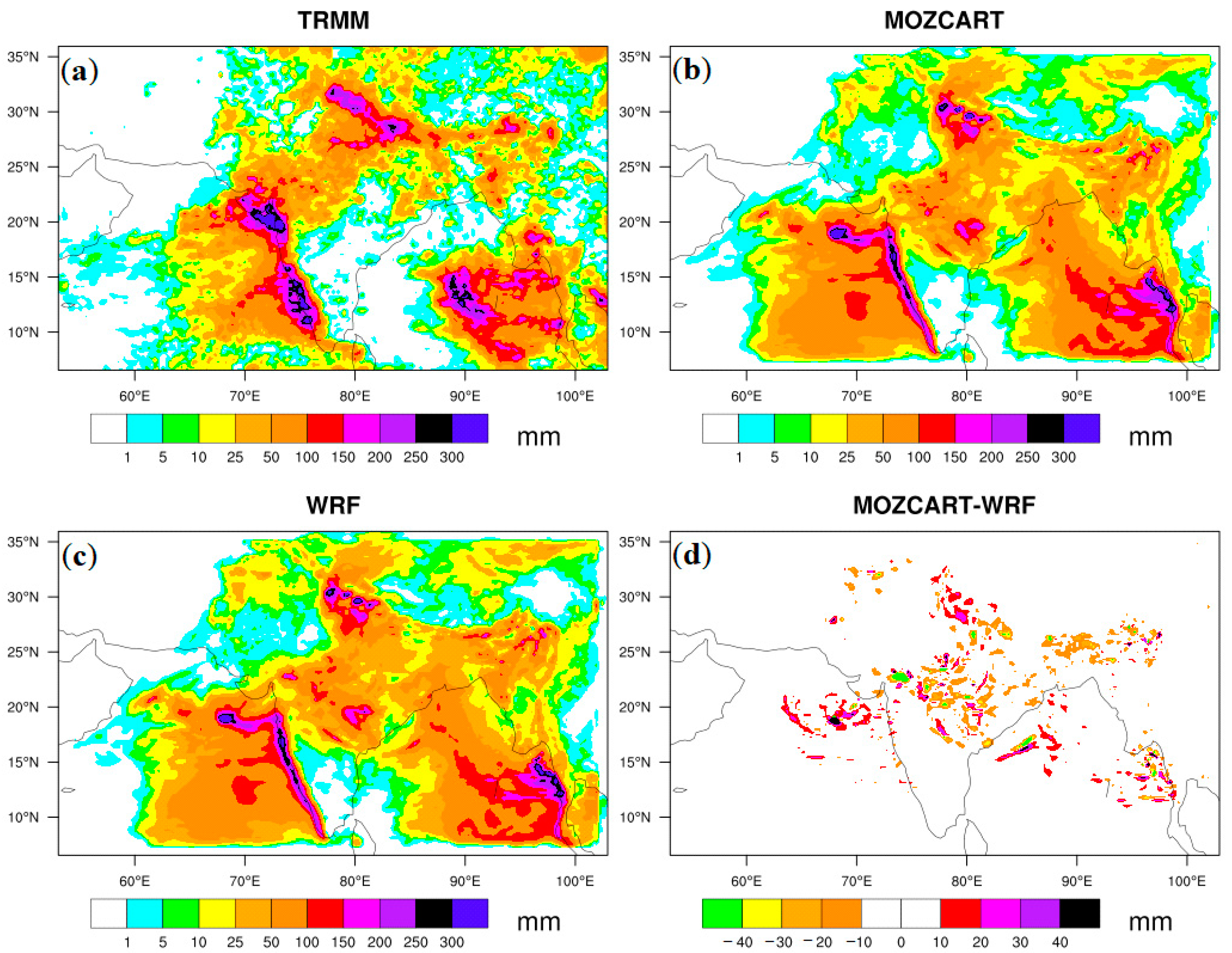
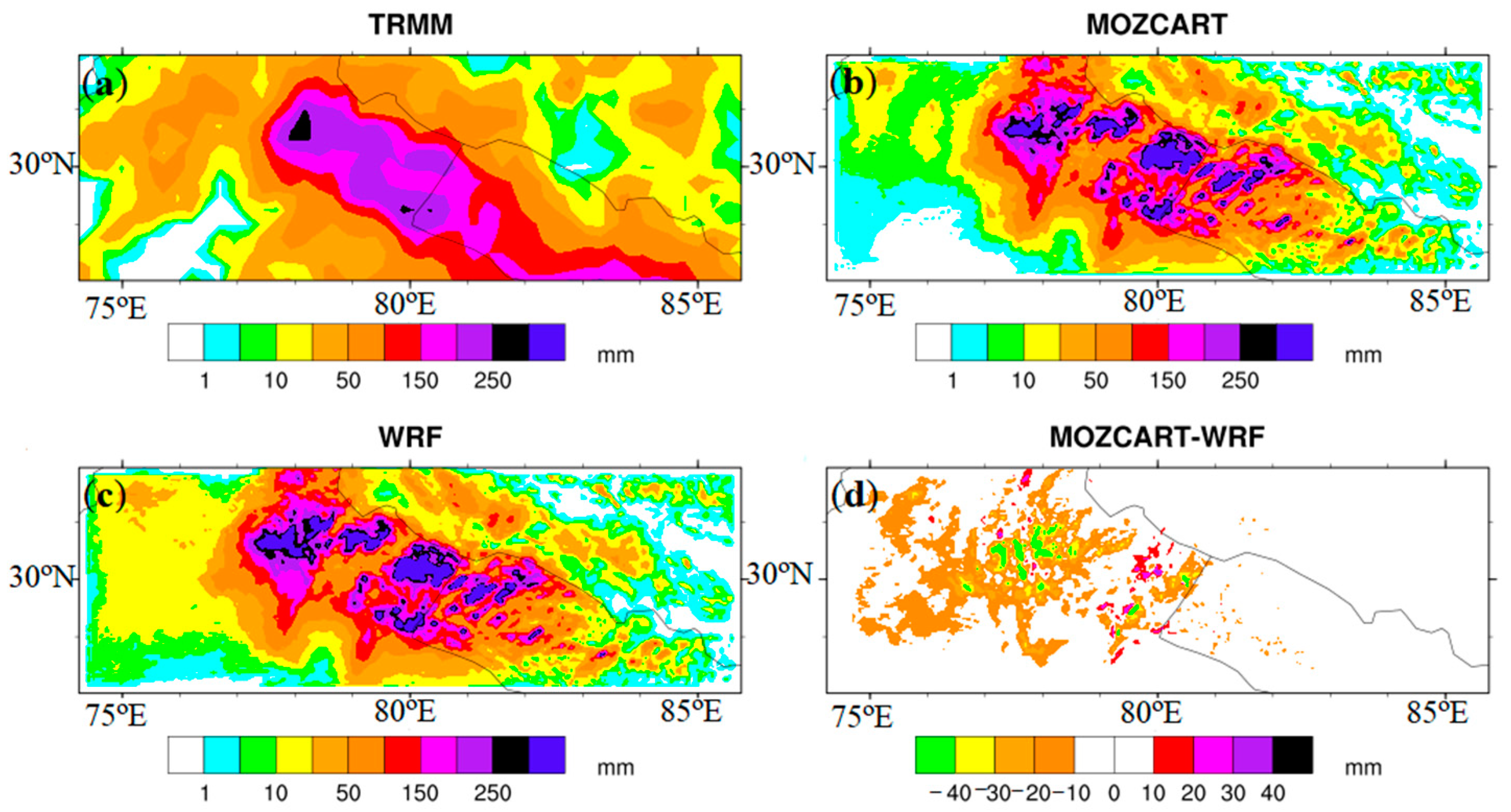
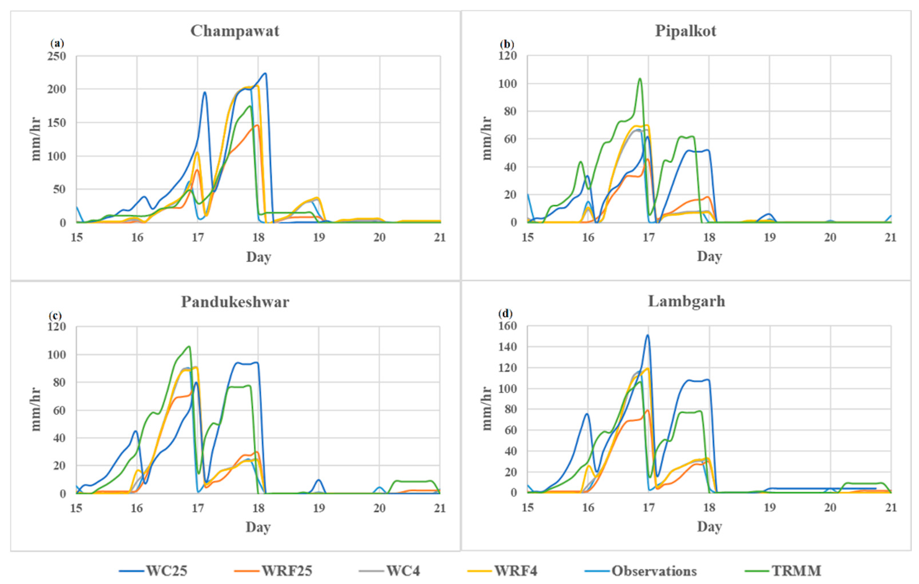
3.1. Precipitation Analysis

Normal rain was reported during 2013 monsoon season throughout India, except a few states of India such as Bihar, Arunachal Pradesh, and Jammu [25]; however, an excess of rain was reported over most of India in June 2013, except for in northeast India. Uttarakhand faced more than a 191% excess of rain during the month of June, which was the highest compared to any other state, while the overall monsoon season recorded only 12% excess rain. As per IMD records, more than 13 districts of Uttarakhand recorded excess rain during June 2013, which was an unusual event in the month of June [22].
This study used the TRMM monthly surface rain rate data product (TRMM_3A12) from January 1998 to December 2014 to determine the rain pattern in Uttarakhand, a state of India, and over Kedarnath, a Himalayan Mountain city. The year 2013 was a neutral year in terms of El Niño and La Nina. An analysis of seasonal and annual average precipitation over Uttarakhand for the year 2013 suggested that it was an average year in terms of accumulated precipitation when compared to other years from 1998–2014. On the other hand, the monthly analysis suggested that in 2013, the month of June observed the highest precipitation compared to any other year. The area-averaged rain rate taken from a few horizontal grids over Kedarnath suggests that seasonal and annual rain rate for the year 2013 was average during the analysis period, whereas the rain rate was higher compared to the state of Uttarakhand. The Kedarnath grid suggests that the rain rate during the month of June and the monsoon season of 2013 was the highest compared to any other year from 1998–2014 (Table S1 and Figure S2).
Figure 1 shows the results of 3 days of accumulated rain (from 16–18 June 2013) over the simulation domain from TRMM and different versions of the WRF model. TRMM accumulated rain (Figure 1a) shows heavy precipitation (greater than 100 mm) over the western coast, northern India, western Nepal, and the area near the southeastern Bay of Bengal. Figure 1b shows accumulated precipitation from the WRF WC25 simulation. The model reproduces major precipitation when compared to the TRMM precipitation results, with some minor differences. Figure 1c shows accumulated rain from WRF25 simulation, which again is similar to the TRMM observations with minor differences. Figure 1d shows the difference in the accumulated rain produced by the WC25 to WRF25 simulation. The results show that precipitation is reduced in the central and northeastern parts of India with the chemistry option turned on. However, northern India (majorly Uttarakhand), over the Arabian Sea and Bay of Bengal, shows increased rain in WC25.
Similar results are seen for the 4 km resolution model simulations (Figure 2). WRF with MOZCART chemistry (WC4) and WRF without chemistry (WRF4) show similar features of accumulated rain when compared to each other, while there are differences when compared to the results obtained from TRMM. It must be noted that grid resolution between the model simulation and the TRMM observations also leads to some of the observed differences. Most of the area that is focused on in the study shows a decrease in precipitation from the simulations with chemistry turned on, whereas few areas also show an increase in precipitation. Both sets of simulations (25 km and 4 km) show the effect of aerosols on precipitation amount in either direction (i.e., increase or decrease). WC25 shows that most of the area over and near Uttarakhand produces more rain in the presence of aerosols, while WC4 shows less rain in the presence of aerosols, except for in a few concentrated places.
Using a combination of different parameterization schemes in WRF simulations, the study by Chawla et al. (2018) shows that most of the combinations were able to capture spatial precipitation features for 15–18 June 2013 as they appear in TRMM with some differences [24]. A previous study using WRF-Chem simulation by Kedia et al. (2018) suggests a 20% increase in precipitation over Uttarakhand due to chemistry, which was determined using a 15-day average simulation and by observing rain over the region for analysis [4]. Average precipitation and other parameters for 15 days were shown as aggregates illustrating the impact of aerosols; however, this was illustrated without providing temporal resolution for the event. Thus, it is difficult to compare our results with previous research [4].
Figure 3 presents a time series of precipitation at four stations in the Himalayan Mountains of Uttarakhand from 15–20 June 2013. These four stations are the nearest present stations to Kedarnath. In situ observation at all four stations shows that precipitation starts from the morning of the 16 and ends on the morning of the 18. A similar trend is observed through satellites for the same time period. All four model simulations can correctly predict the start and end pattern of precipitation and peaks in precipitation with some minor temporal shifts. At all the four stations, WC25 shows early rain, whereas WRF25 shows delayed rain when the models are compared to each other. Both WC4 and WRF4 show delayed rain matching with each other and also match with the WRF25 simulation trend but predict higher rainfall compared to WRF25 for the peak rain during these days. WC25, however, better matches with the TRMM observations compared to other simulations regarding the timing of the rainfall. The study by Castorina et al. (2021) suggests an explicit resolution of the convective system and provides better simulation for extreme events. As the horizontal dimension of convective clouds varies from 0.1 km–10 km and considering that our model resolution (5 km in their study) is much higher than that, the physical parameterization of the convective system can improve the simulation [43]. However, our simulation with convective parameterization shows that the accumulated rain at 25 km and 4 km is in a similar range with some differences, which justifies the role of the parameterization of the convective system in the simulation of extreme events.
Supporting Table S2 shows the coefficient of determination (R2) between TRMM, during in situ observation, and all four simulations with the observations for the period from 15–20 June 2013. Over Kedarnath, the TRMM and model simulations show a low R2 value (0.36–0.41). At other places, TRMM and in situ data show R2 in the range of 0.32–0.60; R2 for TRMM and model ranges between 0.32–0.95, except for Dehradun. The R2 between in situ observation and the models ranges between 0.23–0.93, except for Jolly Grant. The R2 at Jolly Grant between TRMM and in situ observation is 0.60, and between the observation and the model, it is less than 0.31. Observed accumulated rain at Jolly Grant was as high as 200 mm/day (in situ); the model produces less than 100 mm/day during event days, and the model also does not perform well at Dehradun station. Over other stations, the model replicates the strength and period of precipitation. An observation-based report from IMD presents heavy precipitation on 16 and 17 June 2013 [25], which is evident in all model simulations and satellite observations as well (Figure 3). Other observation studies also show heavy precipitation on 16 and 17 June over most of the Uttarakhand region [22,23,26,44].
Figure 1, Figure 2 and Figure 3 suggest that all model simulations adequately capture the spatial and temporal coverage of precipitation, with some differences in the amount of precipitation. WC25 and WRF25 show up to a 50 mm/day rain difference at some of the stations, whereas WC4 and WRF4 show a negligible precipitation difference. Additional analysis suggests more rain in the 25 km simulation without chemistry at Dhanauri (~20 mm/day), Jolly Grant (~60 mm/day), Dehradun (~70 mm/day), and Mandal (~100 mm/day). However, more rain is produced in the 25 km simulation with chemistry in places such as Kedarnath (~40 mm/day), Champawat (~60 mm/day), Nainital (~15 mm/day), Lambagrh (~40 mm/day), Pandukeshwar (~10 mm/day), and Pipalkoti (~20 mm/day). WRF and WRF-Chem were able to simulate precipitation well over most of the observation stations, which is further corroborated by the TRMM observations. Given the model’s ability to replicate the rainfall over Uttarakhand, we present the model-based analysis of monsoon dynamics, cloud properties, and aerosols during this event.

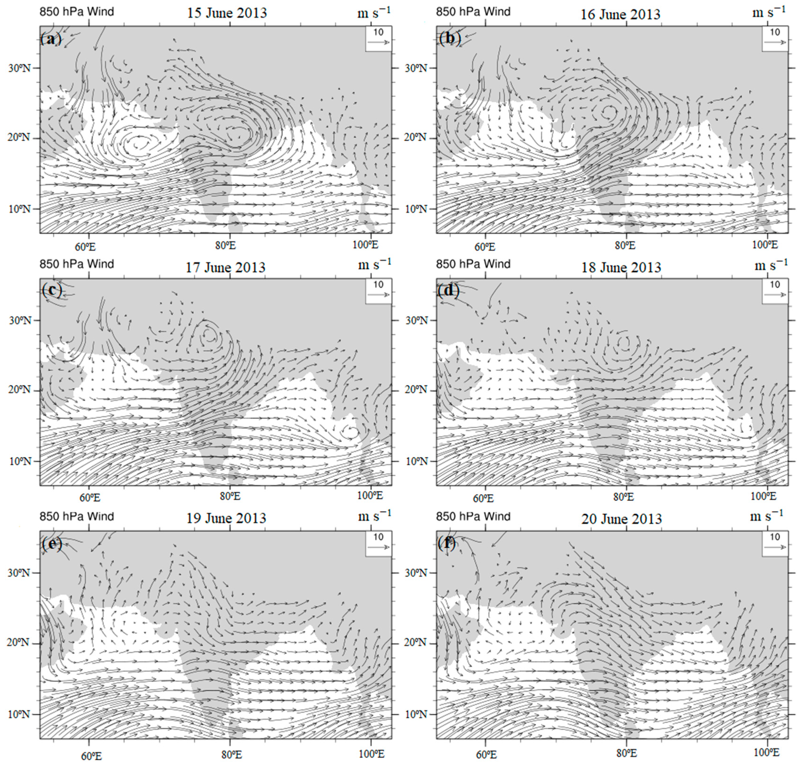
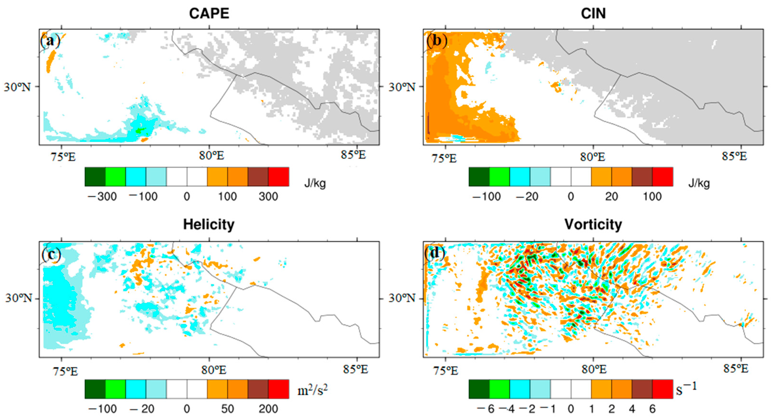
3.2. Monsoon Dynamics
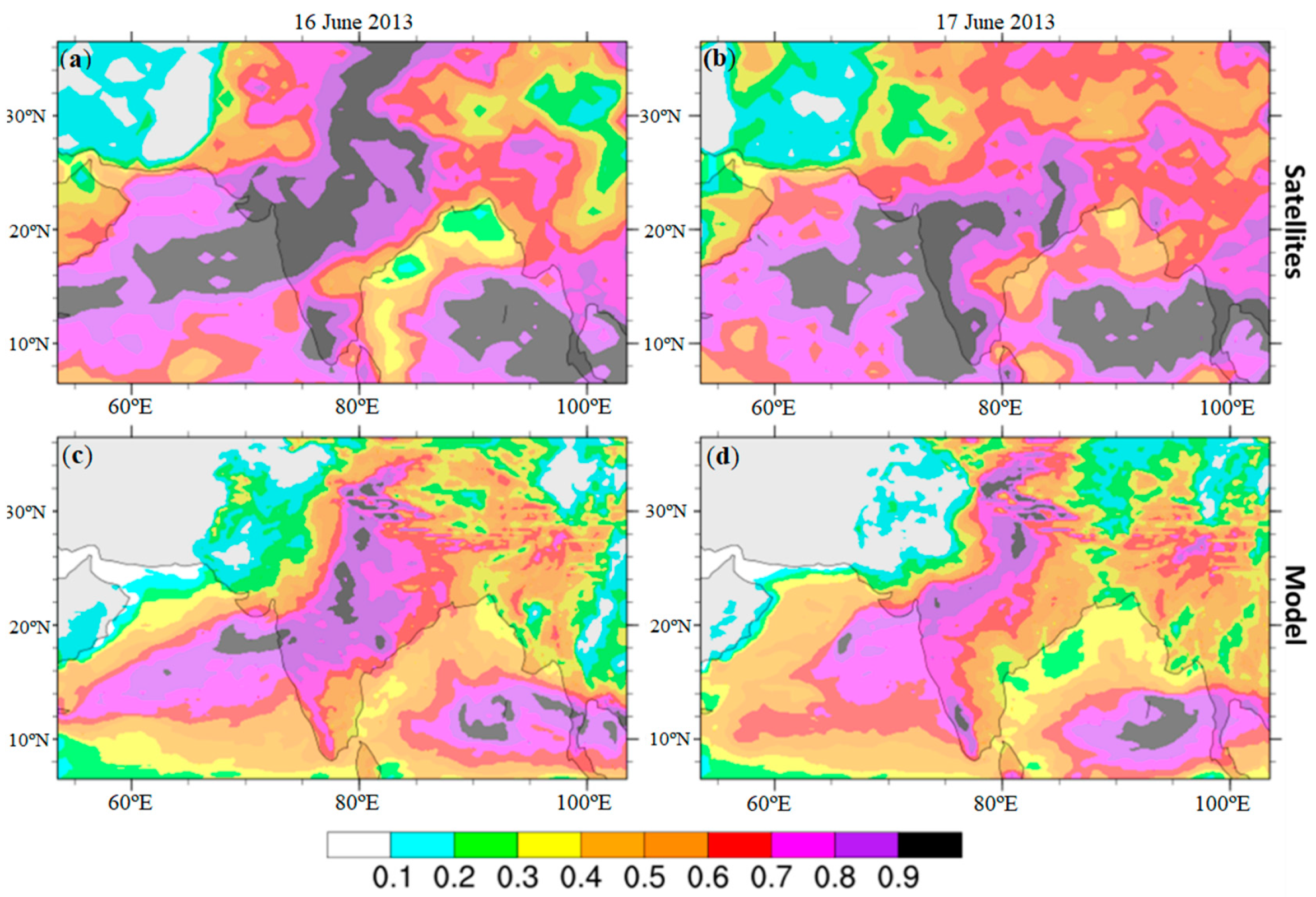
The Indian Meteorological Department, India, and the Department of Hydrology and Meteorology (DHM), Nepal, reported the onset of the summer monsoon on 15 and 14 June 2013, respectively. Due to low heat (high temperature leads to low-pressure zone) over northern India and the high-pressure zone over the adjacent ocean, moisture moves with the wind from the ocean to northern India during monsoons. Figure 4a,b shows the counterclockwise cyclonic motion of the wind direction, implying a strong low pressure (WC25 due to full chemistry option) zone over northern India on 15–16 June, which guided the moisture from the ocean towards the land. WC4 shows consistent winds flowing from southeast to northwest (Figure not shown). Figure 4c shows a low-pressure zone on the 17, which is moving towards the north. The same low-pressure zone further moved towards western Nepal (Figure 4d) on the 18, which created a flood situation in western Nepal (https://www.icimod.org/?q=10932, accessed on 1 April 2021); after the 19 this system disappeared (Figure 4e,f).
Singh and Chand, (2015) have shown the presence of a low-pressure zone over central India (Rajasthan and Madhya Pradesh), as simulated by their model on 16 June. Ray et al. (2014) reported the presence of a low-pressure system during the 16 and 17 over central India [23,25]. The dynamic interaction of the monsoon due to the low-pressure system over central India with the mid-latitude western disturbance results in heavy rainfall [23,25,45]. Similar wind patterns and low-pressure were simulated in all the simulations. The precipitation pattern was also simulated well in the simulations concerning observations and the previous literature.
In situ observations for all of the stations listed in the supporting table shows low pressure near the surface, about 4–6 hPa less than the average atmospheric pressure on the 17. The WC4 and WRF4 simulations represent better pressure at different stations in comparison to simulation WC25 and WRF25, mainly due to a higher model resolution that is better able to reflect topography height. Low pressure indicates an unstable atmosphere and a higher probability of precipitation. High surface relative humidity (≥90%) was observed during the 16 and 17, and the model also simulated high relative humidity for all of the stations (≥80%). Persistent higher humidity indicates a higher probability of precipitation in that area. Observations and the models both showed a rapid decrease in relative humidity from the morning of 18 June. The observed surface temperature on 17 June at all stations fell (~3 °C–5 °C) compared to the average temperature. Similarly, WC25 and WRF25 show temperature falls of ~4 °C–6 °C, while WC4 and WRF4 show a fall of ~2 °C–6 °C. All of the parameters show normal atmospheric conditions from the morning of 18 June in comparison with the event days. Literature based on observations shows 70–100% humidity, low pressure, and low wind during event days over Kedarnath [22].

3.3. Cloud Property

Figure 5 shows the average cloud fraction (CF) from the MODIS (Aqua and Terra) satellites (a,b) and the average model simulated cloud fraction (c,d) for 16 and 17 June 2013. Both the satellites and the model show similar features on 16 (Figure 5a,c): dense clouds from the Arabian Sea to northern India passing through central India along with some dense clouds in the southeastern Bay of Bengal. Both the satellites and the model-based observations show that all of Uttarakhand and western Nepal were covered by dense clouds on the 16. On the 17, the satellites do not show a dense cloud fraction over Uttarakhand and western Nepal, whereas the model does simulate dense cloud fraction over the area. However, on the 17, the satellite data do show similar cloud fraction features over the Western Ghats, Arabian Sea, and Bay of Bengal, as seen on the 16.
Model analysis reveals that the entirety of the Arabian Sea, Bay of Bengal, and central India is covered with low and mid-level clouds (Figure not shown). In this study, low cloud cover is considered up to 800 hPa, medium cloud cover is below 450 hPa, and high cloud cover is above 450 hPa. Along with low- and mid-level clouds, Uttarakhand, Western Nepal, a small part of the Arabian Sea, and the Bay of Bengal were covered with dense high-level clouds on 16 and 17 June. The satellites observed low cloud top pressure (CTP) over Uttarakhand compared to surrounding areas (~300 hPa) on the 16 and (~400 hPa) on 17, indicating the presence of high-level cloud cover over Uttarakhand.
Low cloud top temperature (CTT) was observed from the satellites (~−30 °C to −40 °C) on the 16 and (~ −20 °C to −30 °C) on the 17 over Uttarakhand and western Nepal. CTT from the model simulation was lower in comparison with Uttarakhand and western Nepal (~−10 °C to −20 °C) on both days. WC4 simulates further cooler CTT on the 17 (~−30 °C to −40 °C). The presence of aerosol mostly produced warmer cloud top at WC25, except in some places near Kedarnath, and WC4 simulated changes in CTT variation (±15 °C). Lower CTP and CTT indicate deep cloud with a high amount of precipitation [14].
At 25 km resolution, the presence of aerosols affected the cloud fraction by ±25% away from the major sources of emission (inferred from Figure 1d). The presence of aerosols simulated more clouds at a low level, whereas a decrease was simulated in the high-level clouds, while the mid-level clouds were affected in both ways over the domain of the simulation. Similar results were simulated at the 4 km resolution with and without aerosols for both days. The presence of aerosols played a role in creating warm clouds in the central and eastern parts of India, the same region where the aerosols negatively affected precipitation (Figure 1d). Satellite data along with the model show low CTT and CTP over Kedarnath during the 16 and 17 compared to previous days. The model indicates the presence of dense high clouds over Kedarnath, which could result in a heavy downpour.

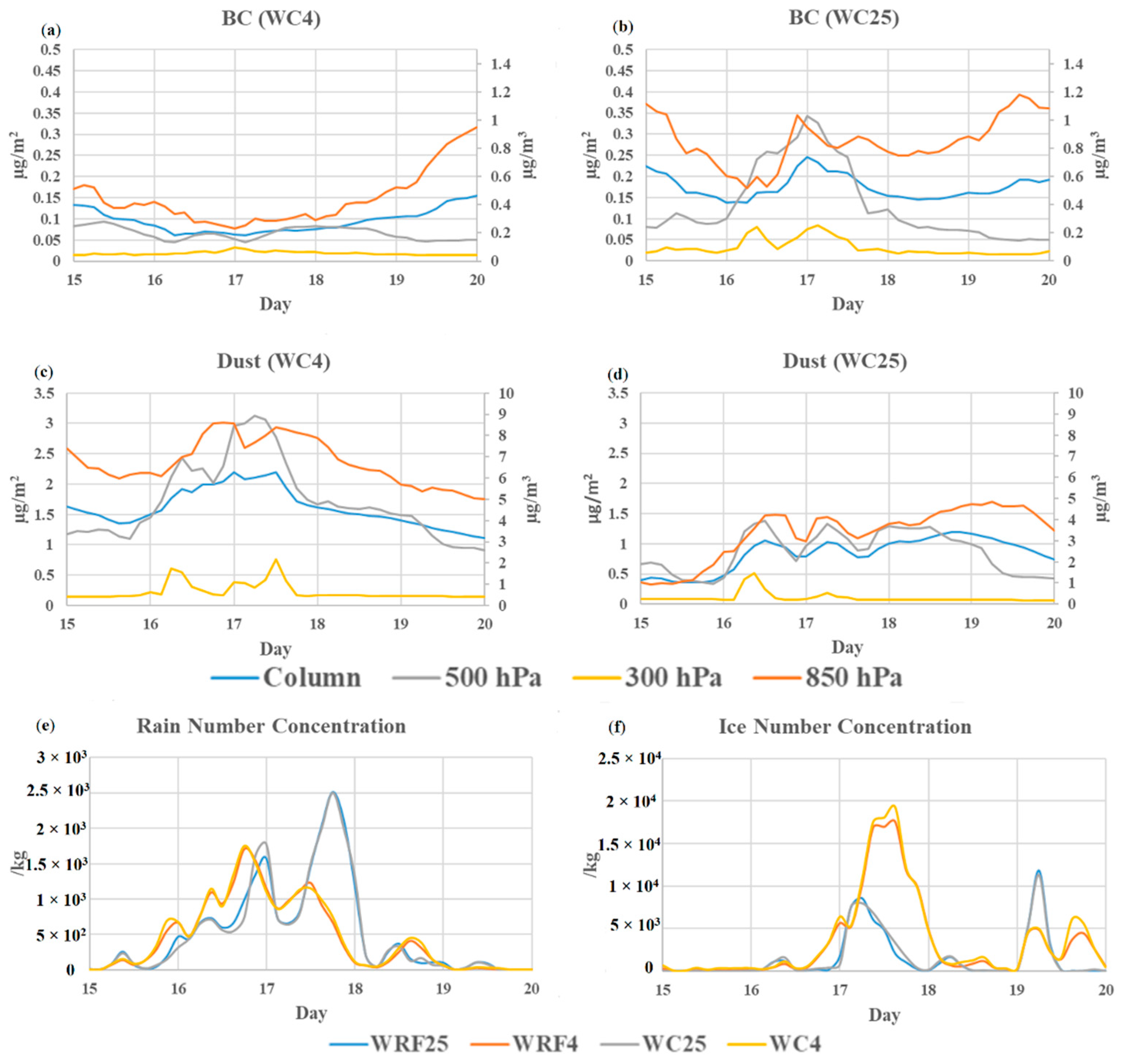
3.4. Aerosol Concentration

Satellite and model analysis suggests the presence of dense high-level (above 6 km) clouds over Kedarnath, so we analyzed aerosols above 6 km (above ~500 hPa). Our results show that over Kedarnath, there is an elevated concentration of anthropogenic and natural aerosols at high altitudes during the event days. Figure 6a,b shows area average concentration of black carbon (BC), and Figure 6c,d shows dust over Uttarakhand (~29–31° N, ~78–81° E) from the 15–19. The night of the 17 shows the highest BC concentration at 500 hPa (>0.25 µg/m3) and above in WC25, whereas it was (>0.05 µg/m3) in the WC4 simulations; the columnar average BC concentration was higher by ~0.1 µg/m3 in WC25, whereas it was lower in WC4 from the previous day. Figure 3 shows that a precipitation peak was present for a similar period over most of the stations. Similarly, natural aerosol dust shows a higher concentration at 500 hPa and above in both the WC4 and WC25 simulations (Figure 6c,d). The previous study on the vertical transport of aerosols during volcanic eruption suggests that WRF-Chem simulates the process quite realistically [46,47]. Similarly, the model-based previous study demonstrates that WRF-Chem realistically simulates vertical aerosol transport during deep convection events [33].
Other bulk aerosol species such as organic carbon (OC), dust (different size), sea salt (different size), and sulfates show similar elevated peaks at 500 hPa and above. Table 2 presents the differences in the concentrations of various aerosol species at 850 hPa, 500 hPa, 3 hPa, and the total column average. The methodology for calculating the differences in the concentrations is as follows:
For all of the aerosol species BC, OC, dust (all sizes), sea salt (all sizes), and sulfates (sulf), we subtracted area average concentration over Uttarakhand (~29–31° N, ~78–81° E) on the event dates (16 or 17) to the nonprecipitating dates (15, 18, 19 and 20) at different pressure levels (column, 850 hPa, 500 hPa, and 300 hPa).
Change in aerosol concentration (ΔX) = area average concentration (non-precipitating days) − area average
concentration (event day)
Most of the bulk aerosol species BC, OC, dust, and sea salt show elevated concentration at 850 hPa and above, especially at the higher elevation of 500 hPa. DUST5 decreases while Sea Salt4 and Sea Salt1 increase insignificantly on the 16 and 17 at all elevations. The near-surface (850 hPa) concentration of DUST4, BC, and OC decreases during heavy precipitation events. At 500 hPa and above, BC, OC, DUST2, 3, 4, and SEA SALT2, 3 increase significantly during the precipitation event days. Sulfate concentration was less in a column and was near the surface, whereas at 500 hPa and above, the concentration was significantly higher during the 16–17 (Table 2). Similar results are observed with the 4 km resolution simulation (Supporting Table S3) with a lower ratio of concentration in the vertical layers compared to the 25 km resolution. The previous study on WRF-Chem sensitivity on horizontal resolution and nesting suggests that the boundary layer shows more sensitivity to 1-way nesting than 2-way nesting at a finer resolution [48], whereas the boundary layer plays an important role in atmospheric aerosols and chemistry [49]. A multimodel study suggests that the model performance to simulate aerosols does not depend on resolution, but the basic difference comes with the treatment of aerosols in a model such as that for removal and deposition parameterization [50].
Further analysis at 500 hPa and above suggest that bulk aerosols follow the fast-moving moisture content from the 15 of June from the eastern coast of India to the Himalayan region until 18 June. The concentration of aerosols was much higher than the stable atmospheric conditions in that region. The study suggests the significant uplifting of aerosols in the mid-troposphere during deep convective events as suggested in previous studies [33,49]. Figure S3 shows a lesser concentration of near-surface BC (850 hPa) during the event period, whereas Figures S4 and S5 shows a significant amount of BC over 500 hPa and 300 hPa in the active convective area during the event. Other aerosols also show similar features in the free troposphere. This indicates the strong vertical transport of aerosols during strong convective events over the effective region, which is evident in the BC flow analysis in Figures S6 and S7. That figure shows a strong updraft of BC from the plains towards to the Himalayan region during the event day, with convection anthropogenic and natural aerosol transport significantly above 500 hPa and above, which are further transported through synoptic monsoon motion in the atmosphere.
Aerosols act as IN and CCN, which are responsible for creating clouds and precipitation [12,13]. Model analysis of average columnar rain number concentration (RNC) and ice number concentration (ICC) over Kedarnath (Figure 6e,f), reveals the elevated concentration of RNC during 16 and 17 June, while ICC shows an elevated concentration on the 17 and a smaller peak on the 19. While there is a significant difference between the model simulations at 25 km and 4 km resolution, there is a minimal difference when taking chemistry (i.e., aerosols) into account. On the 16, all of the models simulated a good number of RNC, whereas ICC was not significantly high over Kedarnath. Higher RNC delays the precipitation time, which leads to higher and deeper clouds [18], as observed by the satellites and the model over Kedarnath on the 16 (Figure 5a,b).
On 17 June, above 500 hPa, a significantly high amount of ICC was present (Figure not shown), which justifies a cooler cloud top, as observed by satellites over Kedarnath. RNC, ICC (Figure 6e,f), and precipitation (Figure 3) patterns suggest two events. The first event (peak) before the 17, which was had been continuously increasing since the evening of the 15 to 16 that resulted in a downpour late at night on the 16–17. The second event with the RNC and ICC peak values that were present during the daytime of 17 led to precipitation in the late evening but with a lesser quantity. Our results suggest that a high amount of ICC held the precipitation within the cloud, which then moved with the synoptic circulation towards western Nepal on the 18, resulting in a heavy downpour there.
Analysis of the extinction coefficient profile from WC25 and WRF25 show the higher difference in extinction coefficient between the heights 2 to 8 km (calculated from Equation (1)), whereas RNC significantly increases in presence of aerosols at 4–6 km on both days over Kedarnath. During both days, the ICC decreases significantly in the presence of aerosols. Supporting Figures S8 and S9 shows decreased ICC above 6 km during the 16 and 17. The satellites were not able to capture aerosol optical depth (AOD) during event day, even near the area near the AERONET station (over Kanpur) does not have data; therefore, AOD comparison with observation was not possible. On the 17, CALIPSO shows 3% data availability, and data loss was reported to be due to a ground station anomaly (https://www-calipso.larc.nasa.gov/products/lidar/browse_images/data_event_log.php?s=production&v=V3-30&browse_date=2013-06-17, accessed on 1 April 2021), whereas the 16 and 18 passes were far from the area of interest.
Analysis suggests the presence of anthropogenic and natural aerosols (BC, OC, dust, sulfate, and sea salt) in the free troposphere above 2 km leads to an increase in RNC, which results in more precipitation over the Kedarnath region. The result shows a higher concentration of aerosols at elevated layers negatively affected the ICC numbers, which resulted in more precipitation in the region. Aerosols over the simulation domain affected the clouds and precipitation in either way.
We also considered evaluating the parameters that are important to indicate severe weather such as convective available potential energy (CAPE), convective inhibition energy (CIN), vorticity, and helicity [51,52]. CAPE was simulated high (≥1000 J/kg) over the Bay of Bengal, the Arabian Sea, and many parts of the Indian subcontinent in WC25, whereas the Kedarnath region does not show high CAPE values during the event days. CIN was very less (≤50 J/kg) over most of the area except over Pakistan and northern India (≥100 J/kg) during event days. Strong (≥12 × 10−5/s) vorticity is simulated in models along the low-pressure zone (Figure 3). Strong helicity (≥400 m2/s2) was also simulated over the Arabian Sea and Uttarakhand. The presence of aerosols affected the radiation over the region, which resulted in changes to the above parameters. At 25 km and 4 km, the presence of aerosols shows (≥±300 J/kg) changes in CAPE, (≥±50 J/kg) CIN, (≥±100 m2/s2) helicity, and (≥±6 × 10⁻⁵/s) vorticity values over many parts in the simulation domain. Over Uttarakhand, the presence of aerosols increased ~200 J/kg in CAPE, ~20 J/kg in CIN, up to 100 m2/s2 in helicity, and above 4 × 10⁻⁵/s in vorticity.
In the 4 km simulation, the aerosol effect show changes up to ±200 J/kg in the CAPE value during the event day in the simulation domain. (Figure 7a), CIN values are significantly affected by the presence of aerosols, whereas similar results are simulated at the 25 km resolution simulation (Figure S10a,b). Helicity and vorticity show strong variation in the presence of aerosols over Kedarnath and nearby areas at convection-permitting scale (Figure 7c,d). Helicity and vorticity changes are not very evident at a 25 km resolution (Figure S10c,d). At the convection-permitting scale, variation in the parameters affected by orographic and thermodynamic are more evident than at low-resolution simulations. WRF-Chem based previous studies suggest that the presence of aerosols in the mid-troposphere shows a significant effect on the surrounding environment at regional and local levels, such as changes in near-surface temperature, wind speed, humidity, boundary layer, etc. [49,53].
Results indicate that the presence of aerosols does not only affect cloud and precipitation by acting as CCN and IN but also affects the severe weather indices; CAPE, CIN, helicity, and vorticity show significant changes in presence of aerosols. Over the Uttarakhand and near to Himalayan foothills, CAPE, CIN, helicity, and vorticity significantly increases in the presence of aerosols.

4. Summary and Conclusions

Long-term (1998–2014) analysis of precipitation from TRMM over Kedarnath suggested that heavy precipitation during June over Kedarnath is an unusual event. Analysis shows that June of 2013 experienced the highest precipitation compared to of the month of June in any other year from 1998–2014; otherwise, the year 2013 was recorded as a normal monsoon year. We used six sets of model simulations at 25 km and 4 km resolution (three each), and further analysis was conducted using four sets of simulations (two from each resolution). We dropped two sets of simulations (one from each resolution) since chemistry without aerosols (MOZART) and without chemistry showed no significant difference in the precipitation amount at both resolutions.
All of the model simulations captured the TRMM observed spatial coverage of precipitation with some differences. The presence of aerosols shows a significant increase in precipitation over Kedarnath and nearby areas, whereas the suppressed precipitation over the central and eastern part of India was observed at a 25 km resolution. Aerosols at the convection-permitting scale (4 km resolution) show similar results with more regional variation and differences in precipitation changes due to the presence of aerosols. In situ observations and TRMM data over many stations near Kedarnath show that the model captures the temporal trend and strength of precipitation with some differences. The model captured the consistent movement of the low-pressure system from central India on the 16 to Kedarnath on the 17 and further towards western Nepal on the 18, as reported in the literature, while it dissipated on the 19. Temperature, pressure, and humidity are also well replicated by the model. Cloud properties such as cloud fraction, cloud top temperature, and pressure are also well simulated by the model, as observed from the satellites.
Model simulation shows deep clouds (above 500 hPa) over Kedarnath and some other parts over the ocean on the 16 and 17. Model analysis suggests the presence of aerosols above 500 hPa, which may act as CCN/IC. The high amount of RNC and ICC over Kedarnath on the 16 and 17 suggests the role of aerosols in heavy precipitation events over Kedarnath. Some of the stations showed a 100 mm/day increase in the rain due to the presence of aerosols, most of the stations showed ~ ± 40 mm/day difference. Average profile analysis shows an unusual presence of aerosols over Kedarnath and significant changes in the rain and ice concentration number in the presence of aerosols. The effect of aerosols on precipitation was not only limited to CCN and IN in clouds; aerosol–radiation feedback causes significant alterations in precipitation. Analysis of CAPE, CIN, vorticity, and helicity shows positive radiation feedback in the region where precipitation was high and a negative effect in the area where precipitation was lower (Figure 1d). Himalayan orographic lifting, a fast-moving monsoon due to low pressure generated from 15–18 June 2013, active westerlies, and aerosol effect on cloud formation due to direct CCN/IN and an indirect radiative effect made this event so devastating. Further detailed analysis of such a system is necessary to understand the vertical transport of aerosols and its effect on cloud properties and convection dynamics in the Himalayan region.

Supplementary Materials

The following are available online at https://0-www-mdpi-com.brum.beds.ac.uk/article/10.3390/atmos12091092/s1, Figure S1: (a) Domain of simulation at 25 km resolution, domain of simulation at 4 km resolution (red box), and Kedarnath (black dot), (b) zoom-in for the location of station 1. Kedarnath, 2. Champawat, 3. Pipalkoti, 4. Pandukeshwar, and 5. Lambgarh. Figure S2: Rain rate over Uttarakhand, nearby Kedarnath, and over Kedarnath average for the annual, monsoon, and June precipitation. Figure S3: BC1 concentration at 850 hPa from 14–19 June 2013. Figure S4: BC1 concentration at 500 hPa from 14–19 June 2013. Figure S5: BC1 concentration at 300 hPa from 14–19 June 2013. Figure S6: BC1 volume flow on 17 June 2013, 25 km resolution (gif). Figure S7: BC1 volume flow on 17 June 2013, 4 km resolution (gif). Figure S8: Difference of extinction coefficient, rain, and ice concentration profile over Kedarnath during (a) 16 June and (b) 17 June from the WC25 and WRF25 simulations. Figure S9: Difference of extinction coefficient, rain, and ice concentration profiles over Kedarnath during (a) 16 June and (b) 17 June from WC4 and WRF4 simulations (WC4-WRF4). Figure S10: Effect of aerosols on (a) CAPE, (b) CIN, (c) helicity, and (d) vorticity at 25 km resolution (WC25-WRF25) during 17 June. Table S1: Average rain rate (mm/hr) over Uttarakhand, Kedarnath, and nearby area for the period of 1998–2014 from TRMM. Table S2: R2 of precipitation from different simulation with observed precipitation from in situ and satellite observations. Table S3: Δconcentration for different aerosols and Δ in absolute percentages in model column and at 850 hPa, 500 hPa, and 300 hPa for 16 and 17 June 2013 over Kedarnath at 4 km resolution.

Author Contributions

Data curation, P.S. (Prashant Singh) and B.A.; formal analysis, P.S. (Prashant Singh), P.S. (Pradip Sarawade) and B.A.; writing—original draft, P.S. (Prashant Singh) and B.A.; writing—review and editing, P.S. (Prashant Singh), P.S. (Pradip Sarawade), and B.A. All authors have read and agreed to the published version of the manuscript.

Funding

This research received no external funding.

Institutional Review Board Statement

Not applicable.

Informed Consent Statement

Not applicable.

Data Availability Statement

Most the website links for the publicly available data are provided in their respective places. For model data, if interested, one may contact the corresponding author through email.

Acknowledgments

This study was partially supported by the core funds of ICIMOD contributed by the governments of Afghanistan, Australia, Austria, Bangladesh, Bhutan, China, India, Myanmar, Nepal, Norway, Pakistan, Sweden, and Switzerland. The views and interpretations in this publication are those of the authors. They are not necessarily attributable to ICIMOD and do not imply the expression of any opinion by ICIMOD concerning the legal status of any country, territory, city, or area of its authority or concerning the delimitation of its frontiers or boundaries, or the endorsement of any product. Authors want to acknowledge observational data used in this study is provided by MOSDAC, SAC, ISRO.

Conflicts of Interest

The authors declare no conflict of interest.

References

  1. Dimri, A.P.; Chevuturi, A.; Niyogi, D.; Thayyen, R.J.; Ray, K.; Tripathi, S.N.; Pandey, A.K.; Mohanty, U.C. Cloudbursts in Indian Himalayas: A review. Earth-Sci. Rev. 2017, 168, 1–23. [Google Scholar] [CrossRef]
  2. Das, S.; Ashrit, R.; Moncrieff, M.W. Simulation of a Himalayan cloudburst event. J. Earth Syst. Sci. 2006, 115, 299–313. [Google Scholar] [CrossRef] [Green Version]
  3. Lau, W.K.M.; Kim, K.M.; Shi, J.J.; Matsui, T.; Chin, M.; Tan, Q.; Peters-Lidard, C.; Tao, W.K. Impacts of aerosol–monsoon interaction on rainfall and circulation over Northern India and the Himalaya Foothills. Clim. Dyn. 2017, 49, 1945–1960. [Google Scholar] [CrossRef] [PubMed] [Green Version]
  4. Kedia, S.; Vellore, R.K.; Islam, S.; Kaginalkar, A. A study of Himalayan extreme rainfall events using WRF-Chem. Meteorol. Atmos. Phys. 2018, 131, 1133–1143. [Google Scholar] [CrossRef]
  5. Gautam, R.; Hsu, N.C.; Lau, K.M.; Tsay, S.C.; Kafatos, M. Enhanced pre-monsoon warming over the Himalayan-Gangetic region from 1979 to 2007. Geophys. Res. Lett. 2009, 36. [Google Scholar] [CrossRef] [Green Version]
  6. Ojha, N.; Sharma, A.; Kumar, M.; Girach, I.; Ansari, T.U.; Sharma, S.K.; Singh, N.; Pozzer, A.; Gunthe, S.S. On the widespread enhancement in fine particulate matter across the Indo-Gangetic Plain towards winter. Sci. Rep. 2020, 10, 1–9. [Google Scholar] [CrossRef] [PubMed] [Green Version]
  7. Saikia, A.; Pathak, B.; Singh, P.; Bhuyan, P.K.; Adhikary, B. Multi-model evaluation of meteorological drivers, air pollutants and quantification of emission sources over the upper Brahmaputra basin. Atmosphere 2019, 10, 703. [Google Scholar] [CrossRef] [Green Version]
  8. Seinfeld, J.H.; Carmichael, G.R.; Arimoto, R.; Conant, W.C.; Brechtel, F.J.; Bates, T.S.; Cahill, T.A.; Clarke, A.D.; Doherty, S.J.; Flatau, P.J.; et al. ACE-ASIA: Regional climatic and atmospheric chemical effects of Asian dust and pollution. Bull. Am. Meteorol. Soc. 2004, 85, 367–380. [Google Scholar] [CrossRef]
  9. Devara, P.C.S.; Manoj, M.G. Aerosol-cloud-precipitation interactions: A challenging problem in regional environment and climate research. Particuology 2013, 11, 25–33. [Google Scholar] [CrossRef]
  10. Lebo, Z.J.; Feingold, G. On the relationship between responses in cloud water and precipitation to changes in aerosol. Atmos. Chem. Phys. 2014, 14, 11817–11831. [Google Scholar] [CrossRef] [Green Version]
  11. Stevens, B.; Feingold, G. Untangling aerosol effects on clouds and precipitation in a buffered system. Nature 2009, 461, 607–613. [Google Scholar] [CrossRef]
  12. Andreae, M.O.; Rosenfeld, D. Aerosol-cloud-precipitation interactions. Part 1. The nature and sources of cloud-active aerosols. Earth-Sci. Rev. 2008, 89, 13–41. [Google Scholar] [CrossRef]
  13. Solomos, S.; Kallos, G.; Kushta, J.; Astitha, M.; Tremback, C.; Nenes, A.; Levin, Z. An integrated modeling study on the effects of mineral dust and sea salt particles on clouds and precipitation. Atmos. Chem. Phys. 2011, 11, 873–892. [Google Scholar] [CrossRef] [Green Version]
  14. Lin, J.C.; Matsui, T.; Pielke, S.A.; Kummerow, C. Effects of biomass-burning-derived aerosols on precipitations and clouds in the Amazon Basin: A satellite-based empirical study. J. Geophys. Res. Atmos. 2006, 111. [Google Scholar] [CrossRef] [Green Version]
  15. Bond, T.C.; Doherty, S.J.; Fahey, D.W.; Forster, P.M.; Berntsen, T.; Deangelo, B.J.; Flanner, M.G.; Ghan, S.; Kärcher, B.; Koch, D.; et al. Bounding the role of black carbon in the climate system: A scientific assessment. J. Geophys. Res. Atmos. 2013, 118, 5380–5552. [Google Scholar] [CrossRef]
  16. Khain, A.; Rosenfeld, D.; Pokrovsky, A. Aerosol impact on the dynamics and microphysics of deep convective clouds. Q. J. R. Meteorol. Soc. 2005, 131, 2639–2663. [Google Scholar] [CrossRef] [Green Version]
  17. Koren, I.; Kaufman, Y.J.; Rosenfeld, D.; Remer, L.A.; Rudich, Y. Aerosol invigoration and restructuring of Atlantic convective clouds. Geophys. Res. Lett. 2005, 32, 1–4. [Google Scholar] [CrossRef] [Green Version]
  18. Tao, W.K.; Chen, J.-P.; Li, Z.; Wang, C.; Zhang, C. Impact of Aerosols on Convective Clouds and Precipitation. Rev. Geophys. 2012, 50, 1–62. [Google Scholar] [CrossRef] [Green Version]
  19. Bègue, N.; Tulet, P.; Pelon, J.; Aouizerats, B.; Berger, A.; Schwarzenboeck, A. Aerosol processing and CCN formation of an intense Saharan dust plume during the EUCAARI 2008 campaign. Atmos. Chem. Phys. 2015, 15, 3497–3516. [Google Scholar] [CrossRef] [Green Version]
  20. Rosenfeld, D.; Lohmann, U.; Raga, G.B.; O’Dowd, C.D.; Kulmala, M.; Fuzzi, S.; Reissell, A.; Andreae, M.O. Flood or Drought: How Do Aerosols Affect Precipitation? Science 2008, 321, 1309–1313. [Google Scholar] [CrossRef] [PubMed] [Green Version]
  21. Nandargi, S.; Dhar, O.N. Extreme Rainstorm Events over the Northwest Himalayas during 1875–2010. J. Hydrometeorol. 2012, 13, 1383–1388. [Google Scholar] [CrossRef]
  22. Singh, R.; Siingh, D.; Gokani, S.A.; Buchunde, P.S.; Singh, R.P.; Singh, A.K. Brief Communication: Climate, topographical and meteorological investigation of the 16–17 June 2013 Kedarnath (India) disaster causes. Nat. Hazards Earth Syst. Sci. Discuss. 2015, 3, 941–953. [Google Scholar] [CrossRef]
  23. Singh, C.; Chand, R. Exceptionally heavy rainfall over Uttarakhand during 15–18 June, 2013-A case study. Mausam 2015, 66, 741–750. [Google Scholar]
  24. Chawla, I.; Osuri, K.K.; Mujumdar, P.P.; Niyogi, D. Assessment of the Weather Research and Forecasting (WRF) model for simulation of extreme rainfall events in the upper Ganga Basin. Hydrol. Earth Syst. Sci. 2018, 22, 1095–1117. [Google Scholar] [CrossRef] [Green Version]
  25. Ray, K.; Bhan, S.C.; Sunitha Devi, S. A Meteorological Analysis of Very Heavy Rainfall Event over Uttarakhand during 14–17 June, 2013; India Meteorological Department: Delhi, India, 2014; pp. 37–54.
  26. Shukla, D.P.; Dubey, C.S.; Usham, A.L. Orographic Control of the Kedarnath disaster Orographic control of the Kedarnath disaster. Curr. Sci. 2013, 105, 1474–1476. [Google Scholar]
  27. Satoh, M.; Tomita, H.; Miura, H.; Iga, S.; Nasuno, T. Development of a global cloud resolving model–A multi-scale structure of tropical convections. J. Earth Simulator 2005, 3, 11–19. [Google Scholar]
  28. Grabowski, W.W. Toward Cloud Resolving Modeling of Large-Scale Tropical Circulations: A Simple Cloud Microphysics Parameterization. Am. Meteorol. Soc. 1998, 55, 3283–3298. [Google Scholar] [CrossRef]
  29. Kilaru, A.; Kotamraju, S.K.; Avlonitis, N.; Sri Kavya, K.C. Rain rate intensity model for communication link design across the Indian region. J. Atmos. Sol.-Terr. Phys. 2016, 145, 136–142. [Google Scholar] [CrossRef]
  30. Powers, J.G.; Klemp, J.B.; Skamarock, W.C.; Davis, C.A.; Dudhia, J.; Gill, D.O.; Coen, J.L.; Gochis, D.J.; Ahmadov, R.; Peckham, S.E.; et al. The weather research and forecasting model: Overview, system efforts, and future directions. Bull. Am. Meteorol. Soc. 2017, 98, 1717–1737. [Google Scholar] [CrossRef]
  31. Skamarock, W.C.; Klemp, J.B.; Dudhi, J.; Gill, D.O.; Barker, D.M.; Duda, M.G.; Huang, X.-Y.; Wang, W.; Powers, J.G.; Dudhia, J.; et al. A Description of the Advanced Research WRF Version 3; NCAR Techical Note-475+ STR; NCAR: Pod, CL, USA, 2008. [Google Scholar] [CrossRef]
  32. Grell, G.A.; Peckham, S.E.; Schmitz, R.; Mckeen, S.A.; Frost, G.; Skamarock, W.C.; Eder, B. Fully coupled “online” chemistry within the WRF model. Atmos. Environ. 2005, 39, 6957–6975. [Google Scholar] [CrossRef]
  33. Singh, P.; Adhikary, B.; Sarawade, P. Transport of black carbon from planetary boundary layer to free troposphere on a seasonal scale over South Asia. Atmos. Res. 2020, 235, 104761. [Google Scholar] [CrossRef]
  34. Janssens-Maenhout, G.; Dentener, F.; Van Aardenne, J.; Monni, S.; Pagliari, V.; Orlandini, L.; Klimont, Z.; Kurokawa, J.; Akimoto, H.; Ohara, T.; et al. EDGAR-HTAP: A Harmonized Gridded Air Pollution Emission Dataset Based on National Inventories; Commission Publications Office: Spra, Italy, 2012; ISBN 9789279231230. [Google Scholar]
  35. Kain, J.S. The Kain–Fritsch Convective Parameterization: An Update. J. Appl. Meteorol. 2004, 43, 170–181. [Google Scholar] [CrossRef] [Green Version]
  36. Hong, S.-Y.; Noh, Y.; Dudhia, J. A New Vertical Diffusion Package with an Explicit Treatment of Entrainment Processes. Mon. Weather Rev. 2006, 134, 2318–2341. [Google Scholar] [CrossRef] [Green Version]
  37. Dudhia, J. Numerical Study of Convection Observed during the Winter Monsoon Experiment Using a Mesoscale Two-Dimensional Model. J. Atmos. Sci. 1989, 46, 3077–3107. [Google Scholar] [CrossRef]
  38. Thompson, G.; Field, P.R.; Rasmussen, R.M.; Hall, W.D. Explicit Forecasts of Winter Precipitation Using an Improved Bulk Microphysics Scheme. Part II: Implementation of a New Snow Parameterization. Mon. Weather Rev. 2008, 136, 5095–5115. [Google Scholar] [CrossRef]
  39. Mlawer, E.J.; Taubman, S.J.; Brown, P.D.; Iacono, M.J.; Clough, S.A. Radiative transfer for inhomogeneous atmospheres: RRTM, a validated correlated-k model for the longwave. J. Geophys. Res. Atmos. 1997, 102, 16663–16682. [Google Scholar] [CrossRef] [Green Version]
  40. Tewari, M.; Chen, F.; Wang, W.; Dudhia, J.; LeMone, M.A.; Mitchell, K.; Ek, M.; Gayno, G.; Wegiel, J.; Cuenca, R.H. Implementation and verification of the unified noah land surface model in the WRF model. Bull. Am. Meteorol. Soc. 2004, 2165–2170. [Google Scholar] [CrossRef]
  41. Paulson, C.A. The Mathematical Representation of Wind Speed and Temperature Profiles in the Unstable Atmospheric Surface Layer. J. Appl. Meteorol. 1970, 9, 857–861. [Google Scholar] [CrossRef]
  42. Madronich, S.; Weller, G. Numerical integration errors in calculated tropospheric photodissociation rate coefficients. J. Atmos. Chem. 1990, 10, 289–300. [Google Scholar] [CrossRef]
  43. Castorina, G.; Caccamo, M.T.; Colombo, F.; Magazù, S. The role of physical parameterizations on the numerical weather prediction: Impact of different cumulus schemes on weather forecasting on complex orographic areas. Atmosphere 2021, 12, 616. [Google Scholar] [CrossRef]
  44. Mishra, A.; Srinivasan, J. Did a cloud burst occur in Kedarnath during 16 and 17 June 2013? Curr. Sci. 2013, 105, 16–18. [Google Scholar]
  45. Sikka, D.R. Synoptic and Meso-Scale Weather Disturbances over South Asia during the Southwest Summer Monsoon Season, 2nd ed.; Chang, C.-P., Ding, Y., Lau, N.-C., Johnson, R.H., Wang, B., Yasunari, T., Eds.; World Scientific: Singapore, 2010; ISBN 9789814343404. [Google Scholar]
  46. Stuefer, M.; Freitas, S.R.; Grell, G.; Webley, P.; Peckham, S.; McKeen, S.A.; Egan, S.D. Inclusion of ash and SO2 emissions from volcanic eruptions in WRF-Chem: Development and some applications. Geosci. Model Dev. 2013, 6, 457–468. [Google Scholar] [CrossRef] [Green Version]
  47. Rizza, U.; Brega, E.; Caccamo, M.T.; Castorina, G.; Morichetti, M.; Munaò, G.; Passerini, G.; Magazù, S. Analysis of the etna 2015 eruption using wrf– chem model and satellite observations. Atmosphere 2020, 11, 1168. [Google Scholar] [CrossRef]
  48. Misenis, C.; Zhang, Y. An examination of sensitivity of WRF/Chem predictions to physical parameterizations, horizontal grid spacing, and nesting options. Atmos. Res. 2010, 97, 315–334. [Google Scholar] [CrossRef]
  49. Singh, P.; Sarawade, P.; Adhikary, B. Carbonaceous aerosol from open burning and its impact on regional weather in South Asia. Aerosol Air Qual. Res. 2020, 20, 419–431. [Google Scholar] [CrossRef] [Green Version]
  50. Eckhardt, S.; Quennehen, B.; Olivié, D.J.L.; Berntsen, T.K.; Cherian, R.; Christensen, J.H.; Collins, W.; Crepinsek, S.; Daskalakis, N.; Flanner, M.; et al. Current model capabilities for simulating black carbon and sulfate concentrations in the Arctic atmosphere: A multi-model evaluation using a comprehensive measurement data set. Atmos. Chem. Phys. 2015, 15, 9413–9433. [Google Scholar] [CrossRef] [Green Version]
  51. Tajbakhsh, S.; Ghafarian, P.; Sahraian, F. Instability indices and forecasting thunderstorms: The case of 30 April 2009. Nat. Hazards Earth Syst. Sci. 2012, 12, 403–413. [Google Scholar] [CrossRef]
  52. Singh, P. Prediction of Potential Thunderstorm Over Ocean near Sriharikota. Int. J. Interdiscip. Res. Innov. 2015, 3, 1–6. [Google Scholar]
  53. Hirtl, M.; Stuefer, M.; Arnold, D.; Grell, G.; Maurer, C.; Natali, S.; Scherllin-Pirscher, B.; Webley, P. The effects of simulating volcanic aerosol radiative feedbacks with WRF-Chem during the EyjafjallajÖkull eruption, April and May 2010. Atmos. Environ. 2019, 198, 194–206. [Google Scholar] [CrossRef]
Figure 1. Three days accumulated rain from (a) TRMM and those from the WRF simulations (b) WC25 and (c) WRF25 and (d) the difference in rainfall between WC25 and WRF25.
Atmosphere 12 01092 g001
Figure 2. Three days accumulated rain from (a) TRMM and the simulation of WRF at a 4 km resolution for (b) WC4 and (c) WRF4 (d) and the difference of rain produced by WC4-WRF4.
Atmosphere 12 01092 g002
Figure 3. Precipitation from different simulations and observations from 15–20 June 2013 for (a) Champawat, (b) Pipalkoti, (c) Pandukeshwar, and (d) Lambgarh.
Atmosphere 12 01092 g003
Figure 4. Daily wind speed at 850 hPa from 15–20 June (af). Simulation WC25.
Atmosphere 12 01092 g004
Figure 5. Average cloud fraction on 16 and 17 June (a) and (b) the MODIS satellites (Aqua and Terra combined) (c) and (d) model, respectively.
Atmosphere 12 01092 g005
Figure 6. (a,b) BC concentration from 15–19 June 2013 at 850 hPa, 500 hPa, 300 hPa, and the columnar average at the 4 km and 25 km resolutions (c,d) for dust. (e) Rain number and (f) ice number concentration with different model simulations.
Atmosphere 12 01092 g006
Figure 7. Effect of aerosols on (a) CAPE, (b) CIN, (c) helicity, and (d) vorticity at 4 km resolution (WC4-WRF4) during 17 June.
Atmosphere 12 01092 g007
Table 1. Domain and parameterization details for different simulations.
SimulationsWC25WRF25WC4WRF4
Centered at22° N, 78° E30° N, 80° E
Resolution25 × 25 km4 × 4 km
No. of grids130 × 203 × 40223 × 555 × 40
Domain6.5–36.0° N, 53.0–103.0° E28–32.0° N, 74.25–85.75° E
Chemistry SchemeMOZCART-MOZCART-
Convective parameterizationKain–Fritsch Scheme [35]
Planetary boundary layer physicsYonsei University Scheme (YSU) [36]
Shortwave radiation physicsDudhia Shortwave Scheme [37]
MicrophysicsThompson graupel scheme [38]
Longwave radiation physicsRRTM Longwave Scheme [39]
Land-atmosphere interactionUnified Noah Land Surface Model scheme [40]
Surface layer optionMM5 Similarity Scheme [41]
PhotolysisMadronich fast-Ultraviolet-Visible Model (F-TUV) [42]
Table 2. Δconcentration for different aerosols and Δ in absolute percentage in model column and at 850 hPa, 500 hPa, and 300 hPa for 16 and 17 June 2013 over Kedarnath at 25 km resolution.
Aerosols16 June 2013
Δ ColumnΔ 850 hPaΔ 500 hPaΔ 300 hPa
ug/m3%ug/m3%ug/m3%ug/m3%
Black Carbon (BC)−0.001−0.56−0.225−25.100.156200.260.029142.23
Organic Carbon (OC)−0.023−2.15−1.672−28.861.038226.530.177240.49
DUST10.68536.862.40940.011.12445.430.35295.92
DUST21.26429.564.89334.382.06938.090.775104.79
DUST30.76626.033.18930.911.38440.550.549137.52
DUST4−0.054−5.85−0.764−17.660.35750.640.149230.30
DUST5−0.031−47.90−0.165−57.98−0.027−39.570.00319.12
SEA SALT10.00893.740.02671.090.015210.090.00241.50
SEA SALT20.075128.650.2271.480.146493.880.0211478.02
SEA SALT30.058152.670.19487.730.083540.520.0113580.23
SEA SALT40.0002873.930.0011653.670.00011481.690.0000143480.71
sulf−0.028−2.82−1.349−28.990.71185.370.12672.73
17 June 2013
Δ ColumnΔ 850 hPaΔ 500 hPaΔ 300 hPa
ug/m3%ug/m3%ug/m3%ug/m3%
BC0.0320.82−0.039−4.360.154197.750.031151.07
OC0.18917.89−0.473−8.170.981214.080.152205.95
DUST10.29816.051.41223.440.48919.750.10829.43
DUST20.61514.373.03321.311.21222.310.22730.63
DUST30.42314.382.06320.000.99929.290.14837.05
DUST4−0.043−4.62−0.773−17.850.38754.910.04264.18
DUST5−0.025−38.44−0.137−48.18−0.012−17.960.001−7.58
SEA SALT10.00893.290.03186.710.011148.710.0019.00
SEA SALT20.077132.310.28491.950.107362.540.009690.37
SEA SALT30.03695.690.13761.890.047307.400.0041261.94
SEA SALT40.0001220.350.0002122.560.00003291.730.0000027656.47
sulf−0.056−5.60−1.087−23.370.40548.550.07341.89
Publisher’s Note: MDPI stays neutral with regard to jurisdictional claims in published maps and institutional affiliations.

