Use and Scalability of OpenFOAM for Wind Fields and Pollution Dispersion with Building- and Ground-Resolving Topography

Abstract

Complex flow and pollutant dispersion simulations in real urban settings were investigated by using computational fluid dynamics (CFD) simulations with the SST $k-\omega$ Reynolds-averaged Navier–Stokes (RANS) equation with OpenFOAM. The model was validated with a wind-tunnel experiment using two surface-mounted cubes in tandem, and the flow features were reproduced with the correct qualitative behaviour. The real urban geometry of the Parade Square in Warsaw, Poland was represented with both laser-scanning data for the ground geometry and the CityGML standard to describe the buildings as an example. The Eulerian dispersion of a passive scalar and the flow behaviour could be resolved within minutes over a computational domain with a size of 958 × 758 m${}^2$ and a height of 300 m with over 2 M cells due to the good and strong parallel scalability in OpenFOAM. This implies that RANS modelling with parallel computing in OpenFOAM can potentially be used as a tool for situational awareness on a local urban scale; however, entire cities would be too large.

1. Introduction

The simulation of intended or unintended atmospheric dispersion in a complex geometry—e.g., in an urban area or industrial site—is necessary for the assessment of hazards. In addition to the characteristics of sources, which are not considered here, the governing factors in such events are the wind speed and atmospheric stability, as well as the interaction with 3D structures, such as buildings and rough terrain. For the purpose of situational awareness, a reliable, fast, and fairly accurate tool is needed in the mitigation of risk, in decision making, and among first responders.

Wind-field modelling is imperative for such capabilities, and computational fluid dynamics (CFD) models have gained increased popularity for phenomena occurring at the street level, such as wind wakes and re-circulation patterns, as people who are at risk can be modelled. Among these models, the Reynolds-averaged Navier–Stokes (RANS) model is the fastest and is, thus, likely a suitable choice for moderately large areas [1]. It involves solving the general equations of fluid dynamics (i.e., the continuity, momentum, and energy equations) together with a turbulence closure in order to approximate the turbulent behaviour of the flow. Large eddy simulations (LESs) offer turbulence modelling that is closer to reality, but at the expense of computational effort. The first-responder tool CT-analyst [2] relies on LES-precomputed wind fields. Back in 2010, some authors stated that it would take about two years to get good coverage of an area [2]. Other authors, on the other hand, claimed that pre-computations on the full parameter set of, e.g., wind speeds, wind directions, and turbulences, would not be realistic, even with RANS [3]. Today, the question of the size of the domain that can be modelled with RANS within the timeframe of a first response remains.

Although CFD and pre-computations may be possible, there are also other non-CFD or hybrid approaches that have been developed for risk mitigation and fast response. For an early review, the reader is referred to [4]. Setting a basis for the field, in 1990, Röckle developed [5] a wind-field model based on the forcing mass consistency for the mean flow together with empirical local wind observations around buildings. This renders a Poisson equation that is computationally feasible to solve. See [6] for an evaluation of the Quick Urban and Industrial Complex (QUIC) model. The downside of this diagnostic approach is the lack of generality for handling arbitrary and complex 3D geometries. Gaussian puff models have also been popular; because they do not explicitly resolve urban topography, efforts have been made to combine them with a mechanistic street network model and Lagrangian stochastic model for dispersion [7], or with SIRANERISK [8], which is an operational model. More recently, an interesting approach was presented in which mega-cities could be modelled based on a forecasted meteorology by combining CFD (RANS) near the source with a diagnostic model for the entire domain; this was referred to as the PMSS modelling system [3].

To investigate the speed achieved by a RANS model in an urban geometry, the popular and open-source CFD environment OpenFOAM [9] was used to solve the system of equations with the shear stress transport (SST) $k-\omega$ [10,11,12] turbulence closure in parallel on a local server with 80 cores. This closure was validated for urban geometries in [13,14], and it is an adequate choice because of its relatively low computational cost. OpenFOAM has support for both compressible and incompressible turbulent flow simulations in 3D, as well as an extensive set of turbulence closures for RANS modelling. Recently, a new suite of atmospheric boundary conditions was added to OpenFOAM (v2006), which made it a good choice for this application.

Herein, OpenFOAM was firstly validated against wind-tunnel data from two surface-mounted cubes in tandem [15], which showed qualitative agreement. The parallel scalability and computational time from the perspective of a situational awareness tool were then investigated with the atmospheric inflow profiles. By using the Parade Square in Warsaw, Poland as an example, a method was devised so that dispersion events could be simulated in complex and real geometries.

2. Materials and Methods

The Navier–Stokes (NS) equations describe the motion of viscous fluids. Consider the NS equations for incompressible flow together with the continuity equation and an equation for turbulent pollutant transport:

$$\begin{array}{cc}\hfill {\partial }_t\mathit{u}+\nabla ·(\mathit{u}\otimes \mathit{u})& =-\frac{1}{{\rho }_0}\nabla p+\nabla ·\nu (\nabla \mathit{u}+\nabla {\mathit{u}}^T)+\frac{1}{{\rho }_0}\mathit{g},\hfill \end{array}$$

(1)

$$\begin{array}{cc}\hfill \nabla ·\mathit{u}& =0,\hfill \end{array}$$

(2)

$$\begin{array}{cc}\hfill {\partial }_{t}c+\nabla \left(c\mathit{u}\right)& =\nabla ·D_c\nabla c+S_c,\hfill \end{array}$$

(3)

where $\mathit{u}$ is the velocity, p is the pressure, $\nu$ is the kinematic viscosity, ${\rho }_0$ is the mass density, g represents body forces, c is the pollutant concentration, $D_c$ is the molecular diffusion of the pollutant, and $S_c$ is a source term. In RANS models, the time averages of velocity ($\overline{\mathit{u}}$), pressure ($\overline{p}$), and concentration ($\overline{c}$) are simulated. Thus, instead of resolving in time, the Reynolds averaging decomposes these quantities into fluctuating and static components or primed and barred notation ($\mathit{u}={\mathit{u}}^{\prime }+\overline{\mathit{u}}$, $p=p^{\prime }+\overline{p}$, and $c=c^{\prime }+\overline{c}$, respectively); in the NS equations, the time-averaged flow description is given as follows:

$$\begin{array}{cc}\hfill \nabla ·(\overline{\mathit{u}}\otimes \overline{\mathit{u}})& =-\frac{1}{{\rho }_0}\nabla \overline{p}+\nabla ·\nu (\nabla \overline{\mathit{u}}+\nabla {\overline{\mathit{u}}}^T)-\nabla ·\overline{({\mathit{u}}^{\prime }\otimes {\mathit{u}}^{\prime })}+\frac{1}{{\rho }_0}\mathit{g},\hfill \end{array}$$

(4)

$$\begin{array}{cc}\hfill \nabla ·\overline{\mathit{u}}& =0.\hfill \end{array}$$

(5)

The pollutant transport is modelled with time dependence in order to to have a framework that accommodates a time-varying source:

$$\begin{array}{cc}\hfill {\partial }_t\overline{c}+\nabla \left(\overline{c}\overline{\mathit{u}}\right)& =\nabla ·D_c\nabla \overline{c}-\nabla ·\overline{\left(c^{\prime }{\mathit{u}}^{\prime }\right)}+S_c.\hfill \end{array}$$

(6)

The fluctuating components remain as cross-terms; for ease of the simulations, the Reynolds stress and turbulent pollutant flux are parameterised with the Boussinesq hypothesis [16]:

$$\begin{array}{cc}\hfill -\overline{({\mathit{u}}^{\prime }\otimes {\mathit{u}}^{\prime })}& ={\nu }_t(\overline{\mathit{u}}\otimes \overline{\mathit{u}})-\frac{2}{3}k\mathbf{I},\hfill \end{array}$$

(7)

$$\begin{array}{cc}\hfill -\overline{\left(c^{\prime }{\mathit{u}}^{\prime }\right)}& =\frac{{\nu }_t}{{\mathrm{Sc}}_t}\nabla \overline{c},\hfill \end{array}$$

(8)

respectively, where ${\nu }_t$ is the eddy/turbulent viscosity and ${\nu }_t/{\mathrm{Sc}}_t$ is the eddy pollutant flux. The turbulent Schmidt number, ${\mathrm{Sc}}_{\mathrm{t}}$, is case dependent and can vary in the range from $0.2$ to $1.3$, but here ${\mathrm{Sc}}_{\mathrm{t}}=0.7$ according to others [17,18].

To close the system of equations, k and ${\nu }_t$ are modelled with the SST $k-\omega$ model [10,11,12]. This model is a blend of the standard $k-ϵ$ model in the free shear flow where it is accurate and the $k-\omega$ in the boundary layer where the standard $k-ϵ$ model otherwise over-predicts the turbulent kinetic energy. The kinetic turbulent energy k and $\omega$ are modelled with the following equations:

$$\begin{array}{cc}\hfill \nabla ·\left(\overline{\mathit{u}}k\right)& =\nabla ·\left(\nu +{\sigma }_k{\nu }_t\right)\nabla k+G-{\beta }^{*}\omega k+S_k,\hfill \end{array}$$

(9)

$$\begin{array}{cc}\hfill \nabla ·\left(u\omega \right)& =\nabla ·\left(\nu +{\sigma }_{\omega }{\nu }_t\right)\nabla \omega +\frac{\gamma }{\nu }G-\beta {\omega }^2-(F_1-1)C{F}_{k\omega }+S_{\omega },\hfill \end{array}$$

(10)

where the terms and default constants for OpenFOAM-v2012 [19] are used. We use a built-in steady-state solver simpleFoam [19] and the simple consistent algorithm [20] for the RANS equations and for the turbulent transport ((6) and (8)); a custom solver was also implemented.

2.1. Boundary Conditions

The turbulent inflow parameters for the simulation of the double-bluff wind-tunnel experiment were set to:

$$\begin{array}{c}\hfill k=\frac{3}{2}{\left(IU\right)}^2,\omega =\frac{k^{1/2}}{{\left({\beta }^{*}\right)}^{1/4}L},\end{array}$$

(11)

with the intensity $I=0.1$ and characteristic length scale $L=0.04$.

For the ABL flow, a logarithmic inflow boundary [21] based on Monin–Obukhov similarity theory was used:

$$\begin{array}{c}\hfill u=\frac{u_{*}}{\kappa }log\left(\frac{z+z_0}{z_0}\right),k=\frac{u_{*}^2}{{\left({\beta }^{*}\right)}^{1/2}},\omega =\frac{u_{*}}{{\left({\beta }^{*}\right)}^{1/2}}\frac{1}{z+z_0},u_{*}=\frac{u_{\mathrm{ref}}\kappa }{ln\left(\frac{z_{\mathrm{ref}}+z_0}{z_0}\right)},\end{array}$$

(12)

where $z_0=0.04$ is a roughness parameter.

For the wall boundary conditions, the velocity field $\overline{u}$ uses a no-slip boundary condition on the ground and buildings. For k using a zero gradient and for $\omega$ and ${\nu }_t$, we use wall functions [19]. Symmetric boundary conditions are imposed for the sides and top boundaries.

2.2. Three-Dimensional Geometry and Computational Mesh

The virtual topography of the Parade Square in Warsaw, Poland was built based on a combination of two data sources: one for the buildings [22] in the CityGML format and a numerical terrain model [23] (NTM) to represent ground roughness. CityGML is the international standard of the Open Geospatial Consortium (OGC) and is based on the Geography Markup Language (GML) [24]. The standard defines a three-dimensional description of cities and regional areas at three different levels of detail (LODs). In this work, LOD = 2 was chosen, since it contains sufficient details for accurate wind-field calculations and dispersion events, but omits details that would make the amount of data very large and too complicated for the generation of a computational mesh. NTM data are based on laser scanning. This dataset was filtered using the ground classification (=2) to exclude, e.g., buildings for which CityGML was a better source. The average height error was not greater than 0.20 m, and the data were at a 1 m spatial resolution in the ground plane in the source. However, they were downsampled to a 5 m resolution to aid in having faster simulations. All geometric operations were performed with the Visualization Toolkit [25] to produce a triangulation of the surfaces that was compatible with the native mesh generator snappyHexMesh in OpenFOAM.

3. Results

3.1. Double Bluff

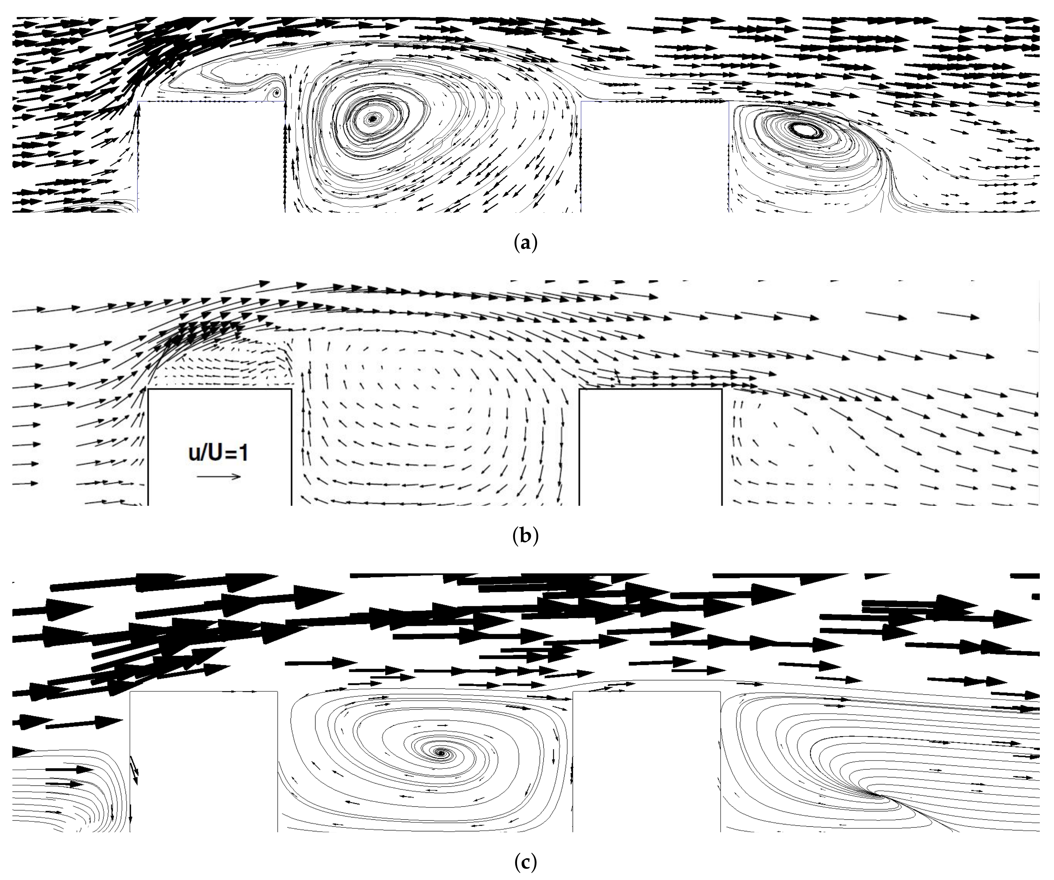
The comparison of the wind-tunnel data of two surface-mounted cubes in tandem [15,26] showed a good agreement between the simulations and experiments. The main features of the mean velocity field (see Figure 1a,b), the front wake at the first cube, the re-circulation zone between the cubes, and the leeward wake of the second cube were present. The lift at the front wall of the first cube eventually dropped down and was re-attached at the roof of the second cube. This model successfully captured the complex flow pattern of a 3D geometry that was similar to that of an urban environment with sharp-cornered buildings. The Reynolds number was $Re$ = 22,000 based on the free-stream velocity of $u=8.8$ m/s, cube dimension of $h=0.04$ m, and viscosity of air of $\nu =1.6\times {10}^{-5}$. Although small geometric differences were reported, this was well above the threshold for the independence of the Reynolds number [27].

3.2. Wind-Field Simulation of a Scaled-Up Double-Bluff Geometry with Atmospheric Inflow Profiles

Simulations of the scaled-up version of the wind-tunnel experiment with cubes (h = 20 m) that were 500 times larger than those in the original experiment are shown in Figure 1c. The Reynolds number ($Re$ = 44) was still above the threshold for the independence of the Reynolds number (=25) [27]. Here, a logarithmic inflow profile was used in comparison with the flat profile in order to simulate the wind tunnel’s geometry; clearly, this had profound effects on the flow characteristics. The re-circulations were still there, but were slightly shifted in their positions. The main difference was that the wind speed was, for the height of the buildings, distinctly lower than in the free stream above the buildings. With a logarithmic inflow, the urban topography effectively acted to shield against the free-blowing wind.

The logarithmic boundary conditions in OpenFOAM were developed for neutral atmospheric stability [28]. Inflow boundary conditions based on Monin–Obukhov similarity theory for the case of stable stratification were employed with RANS modelling and validated in atmospheric dispersion field trials called the Mock Urban Setting Test (MUST) [29]. Much better agreement was found when the inflow turbulent kinetic energy (TKE) was fitted to the upstream values measured [29]. OpenFOAM offers the possibility of fitting the levels of the TKE of the inflow to the measured data and still satisfying the solution to the RANS equations [30]. Nevertheless, it is perhaps more challenging to accurately assess the present atmospheric turbulence (as well as the wind speed and direction). The merging of atmospheric stratification with numerical dispersion modelling is likely a topic for continued future research; a review is provided in [31].

3.3. Warsaw

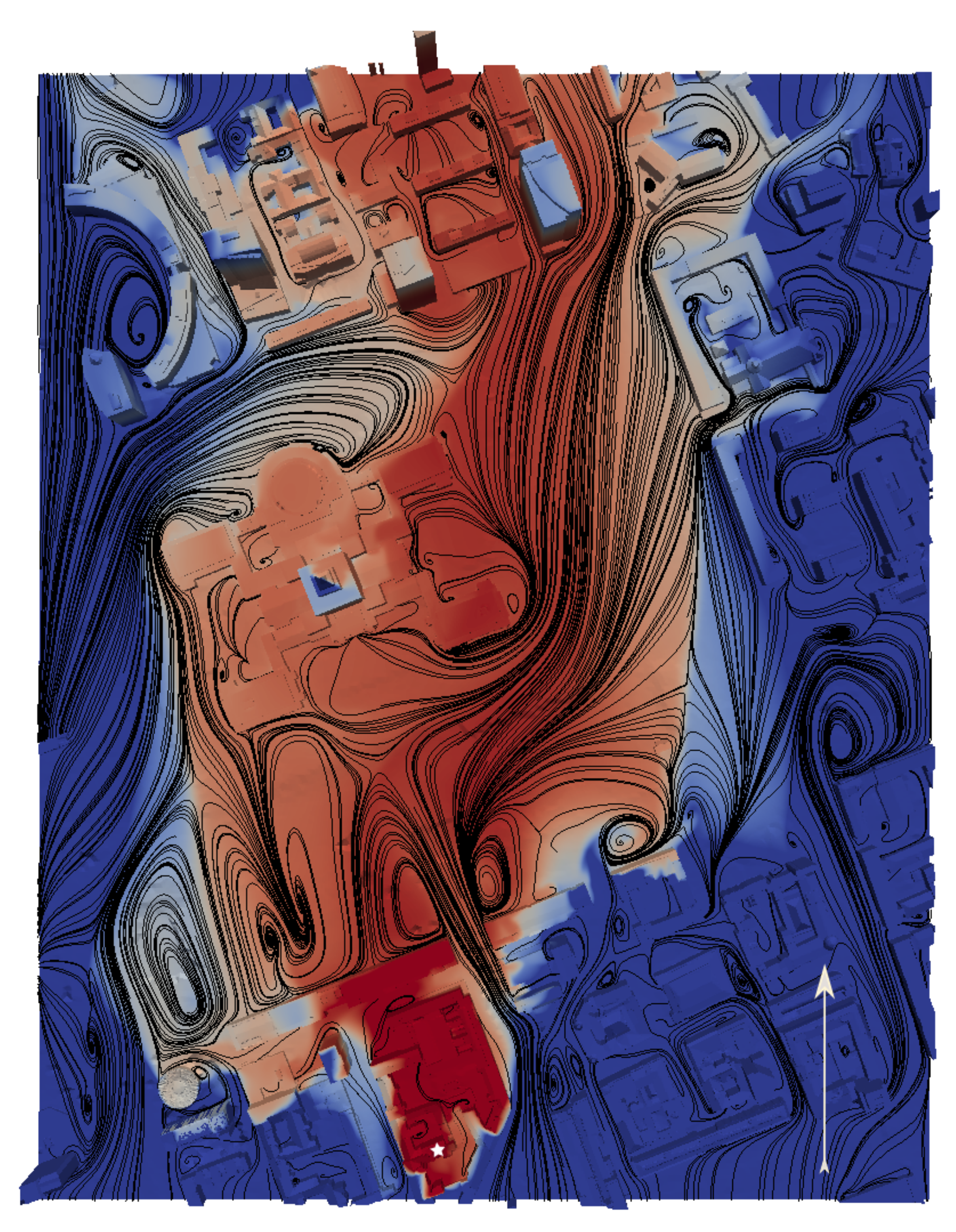
Accurate 3D representations of buildings are needed to simulate the atmospheric properties in the vicinity of those structures. For the Parade Square in Warsaw, the geometry is characterised by a central landmark building in an otherwise open square, followed by several large and tall buildings that are downwind. The upwind regime consists of smaller rectangular buildings. This gives rise to the simulated wind field seen in Figure 2, with several recirculation and deflection zones, as well as separation lines. Clearly, the CFD simulation captures the physical flow behaviour around the central landmark building, as well as the smaller and larger circulations throughout the domain. This complex flow pattern influences the transport of a simulated release. The release point was chosen to be at the rooftop of a smaller building that was upwind (marked by a star in Figure 2) to capture the urban turbulence effects in the close vicinity of the source. The concentration also increases upwind from the source due to the wake patterns, which are similar to the those of the double-bluff experiment. The central building then deflects the transport of the pollutant from the general wind direction as the plume spreads and travels downwind, which is in agreement with the results of other simulations [3] and the MUST field trials [32].

3.4. Parallel Scaling

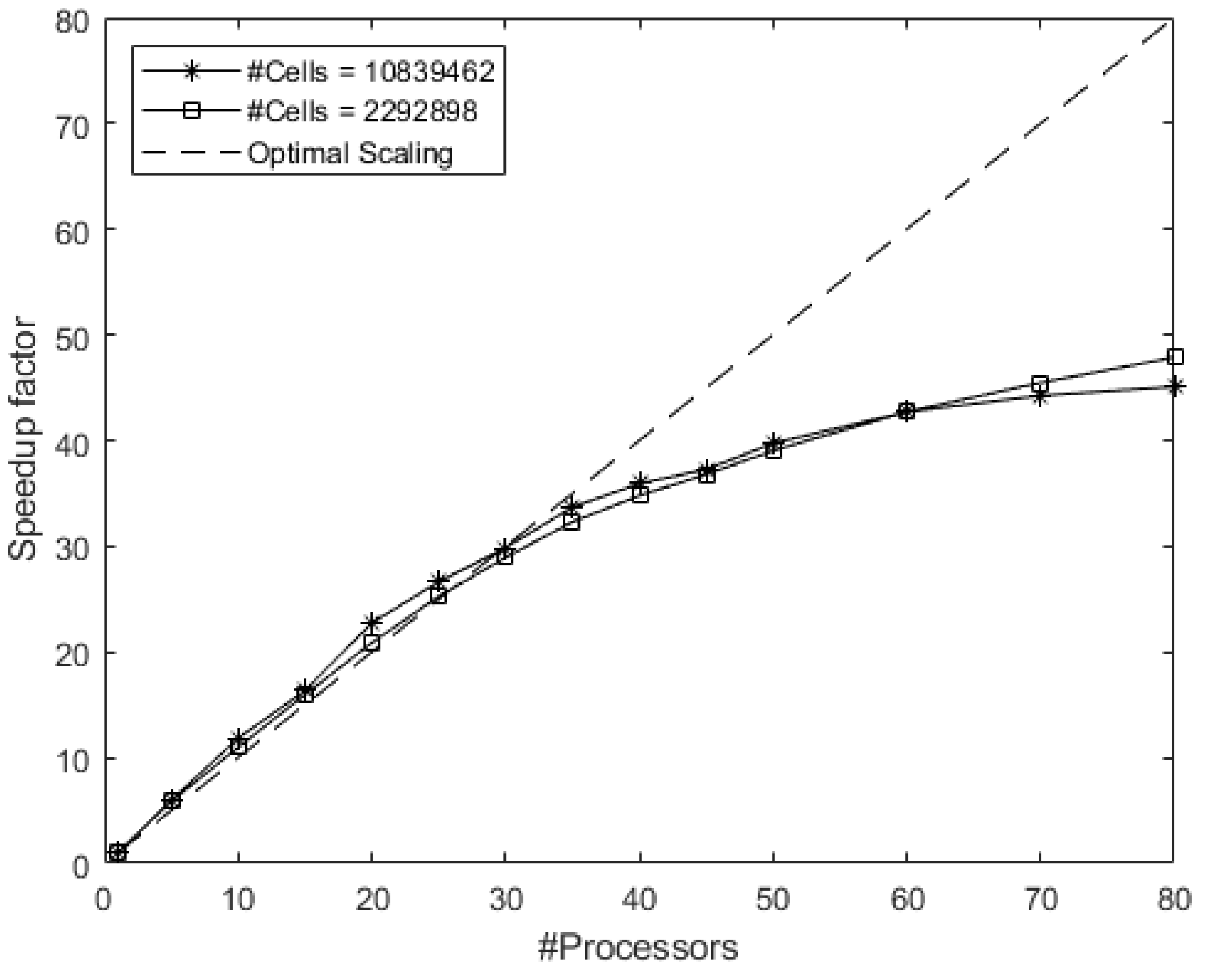
The parallel performance of the RANS turbulence model was investigated on an Intel(R) Xeon(R) Gold 6230 CPU at 2.10 GHz with four sockets containing 20 cores each. The mesh was decomposed using scotch [33], which aims to minimise the number of processor boundaries. Two meshes with different coarseness were produced—one with 10,839,462 and the other with 2,292,898 cells. In both cases, 1000 iterations were performed with the simpleFoam solver in OpenFOAM. The computational domain had a footprint with a size of 958 × 758 m${}^2$ and a height of 300 m.

As seen in Figure 3, for this particular problem, the solver showed good parallel behaviour. A further increase in the processor number would not significantly increase the total clock time. Up to about 35 cores, the solver exhibited strong, excellent scaling for these problem sizes; however, above this number, the communication between different cores became significant. The full capacity of the server gave approximately 135,000 or 28,000 cells for each core to handle, and the total clock time was 954 or 133 s, respectively. To further reduce the computation time, a smaller area or coarser mesh is needed, and the one-minute mark is viable.

From the perspective of situational awareness, this means that with pre-generated meshes, in terms of time, RANS modelling is within the reach of the actions first responders in moderate-sized urban environments. Larger scales that approach the whole of even small cities will currently be too large, considering that the number of cells increases with the size of the footprint modelled at a constant mesh resolution.

4. Conclusions

Here, it was shown that parallel scaling in OpenFOAM increases the speed enough that the wind and dispersion over a local urban environment can be simulated in close to real time with the SST $k-\omega$ Reynolds-averaged Navier–Stokes (RANS) model. Nevertheless, length scales that cover whole cities would still be too time consuming. Building geometry and ground topography can, respectively, be incorporated by using the CityGML standard and laser-scanning data if available.

It is suggested for future work to include validation of the model with a large-scale field experiment. Furthermore, the inflow profiles used here are for neutral stratification, but stable and unstable stratification would also be of interest. The vertical mixing processes can then be further studied for all stratification types, and, since the RANS framework does not seem to be sufficiently fast for large scales, such as whole cities, a more accurate hybrid approach could be foreseen by combining the outcomes from the RANS model with those of either a street network model or a Gaussian puff model, as in [3]. Another possible research direction would be to compare the SST $k-\omega$ turbulence closure to the cheaper zero-equation approach used in [1] for urban geometries.

References

- Gowardhan, A.; Pardyjak, E.; Senocak, I.; Brown, M. A CFD-based wind solver for an urban fast response transport and dispersion model. Environ. Fluid Mech. 2011, 11, 439–464. [Google Scholar] [CrossRef]
- Patnaik, G.; Moses, A.; Boris, J. Fast, Accurate Defense for Homeland Security: Bringing High-Performance Computing to First Responders. J. Aerosp. Comput. Inf. Commun. 2010, 7, 210–222. [Google Scholar] [CrossRef]
- Oldrini, O.; Armand, P.; Duchenne, C.; Perdriel, S.; Nibart, M. Accelerated Time and High-Resolution 3D Modeling of the Flow and Dispersion of Noxious Substances over a Gigantic Urban Area—The EMERGENCIES Project. Atmosphere 2021, 12, 640. [Google Scholar] [CrossRef]
- Brown, M. Urban dispersion—Challenges for fast response modeling. In Proceedings of the 5th AMS Symposium on the Urban Environment, Vancouver, BC, Canada, 23–26 August 2004. [Google Scholar]
- Röckle, R. Bestimmung der Strömungsverhältnisse im Bereich komplexer Bebauungsstrukturen. Ph.D. Thesis, Technical University Darmstadt, Darmstadt, Germany, December 1990. [Google Scholar]
- Kopka, P.; Potempski, S.; Kaszko, A.; Korycki, M. Urban Dispersion Modelling Capabilities Related to the UDINEE Intensive Operating Period 4. Bound.-Layer Meteorol. 2019, 171, 465–489. [Google Scholar] [CrossRef] [Green Version]
- Hertwig, D.; Soulhac, L.; Fuka, V.; Auerswald, T.; Carpentieri, M.; Hayden, P.; Robins, A.; Xie, Z.T.; Coceal, O. Evaluation of fast atmospheric dispersion models in a regular street network. Environ. Fluid Mech. 2018, 18, 1007–1044. [Google Scholar] [CrossRef] [Green Version]
- Soulhac, L.; Lamaison, G.; Cierco, F.X.; Salem, N.B.; Salizzoni, P.; Mejean, P.; Armand, P.; Patryl, L. SIRANERISK: Modelling dispersion of steady and unsteady pollutant releases in the urban canopy. Atmos. Environ. 2016, 140, 242–260. [Google Scholar] [CrossRef]
- Weller, H.G.; Tabor, G.; Jasak, H.; Fureby, C. A tensorial approach to computational continuum mechanics using object-oriented techniques. Comput. Phys. 1998, 12, 620–631. [Google Scholar] [CrossRef]
- Menter, F.R. Two-equation eddy-viscosity turbulence models for engineering applications. AIAA J. 1994, 32, 1598–1605. [Google Scholar] [CrossRef] [Green Version]
- Menter, F.; Esch, T. Elements of industrial heat transfer predictions. In Proceedings of the 16th Brazilian Congress of Mechanical Engineering (COBEM 2001), Minas Gerais, Brazil, 26–30 November 2001; Volume 109, p. 650. [Google Scholar]
- Menter, F.R.; Kuntz, M.; Langtry, R.; Nagano, Y.; Tummers, M.J.; Hanjalic, K. Ten Years of Industrial Experience with the SST Turbulence Model. In Turbulence, Heat and Mass Transfer, 4th ed.; Internal Symposium, Turbulence, Heat and Mass Transfer; Begell House: New York, NY, USA, 2003; Volume 4, pp. 625–632. [Google Scholar]
- Yu, H.; Thé, J. Validation and optimization of SST k-ω turbulence model for pollutant dispersion within a building array. Atmos. Environ. 2016, 145, 225–238. [Google Scholar] [CrossRef]
- Trindade da Silva, F.; Reis, N.C.; Santos, J.M.; Goulart, E.V.; Engel de Alvarez, C. The impact of urban block typology on pollutant dispersion. J. Wind. Eng. Ind. Aerodyn. 2021, 210, 104524. [Google Scholar] [CrossRef]
- Martinuzzi, R.J.; Havel, B. Vortex shedding from two surface-mounted cubes in tandem. Int. J. Heat Fluid Flow 2004, 25, 364–372. [Google Scholar] [CrossRef]
- Schmitt, F.G. About Boussinesq’s turbulent viscosity hypothesis: Historical remarks and a direct evaluation of its validity. C. R. MéCanique 2007, 335, 617–627. [Google Scholar] [CrossRef] [Green Version]
- Tominaga, Y.; Stathopoulos, T. Turbulent Schmidt numbers for CFD analysis with various types of flowfield. Atmos. Environ. 2007, 41, 8091–8099. [Google Scholar] [CrossRef]
- Gualtieri, C.; Angeloudis, A.; Bombardelli, F.; Jha, S.; Stoesser, T. On the Values for the Turbulent Schmidt Number in Environmental Flows. Fluids 2017, 2, 17. [Google Scholar] [CrossRef] [Green Version]
- OpenFOAM: User Guide v2012. Available online: https://www.openfoam.com/documentation/guides/latest/doc/ (accessed on 23 July 2021).
- Doormaal, J.P.V.; Raithby, G.D. Enhancements of the simple method for predicting incompressible fluid flows. Numer. Heat Transf. 1984, 7, 147–163. [Google Scholar] [CrossRef]
- Richards, P.; Hoxey, R. Appropriate boundary conditions for computational wind engineering models using the k-ϵ turbulence model. J. Wind. Eng. Ind. Aerodyn. 1993, 46–47, 145–153. [Google Scholar] [CrossRef]
- Geoportal–Spatial Information for Everyone. Available online: https://www.gov.pl/web/archiwum-inwestycje-rozwoj/geoportal-informacja-przestrzenna-dla-kazdego (accessed on 20 November 2019).
- Geoportal Infrastruktury Informacji Przestrzennej. Główny Geodeta Kraju (eng. “Principal Surveyor of The Country“) Is the Holder of the Data. Available online: http://www.geoportal.gov.pl (accessed on 4 February 2020).
- Gröger, G.; Plümer, L. CityGML—Interoperable semantic 3D city models. ISPRS J. Photogramm. Remote Sens. 2012, 71, 12–33. [Google Scholar] [CrossRef]
- Schroeder, W.; Martin, K.; Lorensen, B. The Visualization Toolkit, 4th ed.; Kitware, Inc.: New York, NY, USA, 2006. [Google Scholar]
- Martinuzzi, R.J.; Havel, B. Turbulent Flow Around Two Interfering Surface-Mounted Cubic Obstacles in Tandem Arrangement. J. Fluids Eng. 1999, 122, 24–31. [Google Scholar] [CrossRef]
- Cui, P.-Y.; Li, Z.; Tao, W.-Q. Numerical investigations on Re-independence for the turbulent flow and pollutant dispersion under the urban boundary layer with some experimental validations. Int. J. Heat Mass Transf. 2017, 106, 422–436. [Google Scholar] [CrossRef] [Green Version]
- Hargreaves, D.; Wright, N. On the use of the k–ε model in commercial CFD software to model the neutral atmospheric boundary layer. J. Wind. Eng. Ind. Aerodyn. 2007, 95, 355–369. [Google Scholar] [CrossRef]
- Milliez, M.; Carissimo, B. Numerical simulations of pollutant dispersion in an idealized urban area, for different meteorological conditions. Bound.-Layer Meteorol. 2007, 122, 321–342. [Google Scholar] [CrossRef]
- Yang, Y.; Gu, M.; Chen, S.Q.; Jin, X.Y. New inflow boundary conditions for modelling the neutral equilibrium atmospheric boundary layer in computational wind engineering. J. Wind. Eng. Ind. Aerodyn. 2009, 97, 88–95. [Google Scholar] [CrossRef]
- Lateb, M.; Meroney, R.; Yataghene, M.; Fellouah, H.; Saleh, F.; Boufadel, M. On the use of numerical modelling for near-field pollutant dispersion in urban environments—A review. Environ. Pollut. 2016, 208, 271–283. [Google Scholar] [CrossRef] [PubMed] [Green Version]
- Yee, E.; Biltoft, C.A. Concentration Fluctuation Measurements in a Plume Dispersing Through a Regular Array of Obstacles. Bound.-Layer Meteorol. 2004, 111, 363–415. [Google Scholar] [CrossRef]
- Pellegrini, F.; Roman, J. Scotch: A software package for static mapping by dual recursive bipartitioning of process and architecture graphs. In High-Performance Computing and Networking; Liddell, H., Colbrook, A., Hertzberger, B., Sloot, P., Eds.; Springer: Berlin/Heidelberg, Germany, 1996; pp. 493–498. [Google Scholar]
Figure 1.
Comparison of the velocity fields of the simulations using the SST turbulence model (a) to experimental wind-tunnel data [15] (b). Simulations with the atmospheric inflow boundaries of the scaled-up geometry are shown in (c); these panels are not to scale. The size of the arrows has been adjusted to aid visualisation, and streamlines have been added to enhance the patterns in which the arrows are small.
Figure 2.
Visualisation of the ground concentration of a pollutant on a logarithmic scale that was released on a roof top (white star), which is in the bottom part of the figure. The complex wind field is visualised using streamlines, and the inflow wind direction is given by the white arrow. The geometry is that of the Parade Square in Warsaw, Poland.
Figure 3.
Parallel scaling using two different mesh sizes of the RANS solver on the real geometry of the Parade Square in Warsaw, Poland.
Publisher’s Note: MDPI stays neutral with regard to jurisdictional claims in published maps and institutional affiliations. |
© 2021 by the authors. Licensee MDPI, Basel, Switzerland. This article is an open access article distributed under the terms and conditions of the Creative Commons Attribution (CC BY) license (https://creativecommons.org/licenses/by/4.0/).
Share and Cite
MDPI and ACS Style
Elfverson, D.; Lejon, C. Use and Scalability of OpenFOAM for Wind Fields and Pollution Dispersion with Building- and Ground-Resolving Topography. Atmosphere 2021, 12, 1124. https://0-doi-org.brum.beds.ac.uk/10.3390/atmos12091124
AMA Style
Elfverson D, Lejon C. Use and Scalability of OpenFOAM for Wind Fields and Pollution Dispersion with Building- and Ground-Resolving Topography. Atmosphere. 2021; 12(9):1124. https://0-doi-org.brum.beds.ac.uk/10.3390/atmos12091124
Chicago/Turabian StyleElfverson, Daniel, and Christian Lejon. 2021. "Use and Scalability of OpenFOAM for Wind Fields and Pollution Dispersion with Building- and Ground-Resolving Topography" Atmosphere 12, no. 9: 1124. https://0-doi-org.brum.beds.ac.uk/10.3390/atmos12091124
Note that from the first issue of 2016, this journal uses article numbers instead of page numbers. See further details here.