
Trends in the Airglow Temperatures in the MLT Region—Part 3: Ground-Based and SABER Measurements


1
Department of Physics, Penn State Lehigh Valley, Center Valley, PA 18034, USA
2
Department of Physics, Penn State University Park, State College, PA 16801, USA
*
Author to whom correspondence should be addressed.
†
Current address: Physics Department, Lehigh University, Bethlehem, PA 18015, USA.
Atmosphere 2021, 12(9), 1161; https://0-doi-org.brum.beds.ac.uk/10.3390/atmos12091161
Submission received: 12 August 2021
/
Revised: 1 September 2021
/
Accepted: 6 September 2021
/
Published: 9 September 2021
(This article belongs to the Section Upper Atmosphere)
Abstract
:Ground-based temperature measurements at Svalbard, Wuppertal, and Hohenpeissenberg were analyzed to obtain F10.7, Ap index, and Dst index trends. The trends were then compared to those obtained from Sounding of the Atmosphere using Broadband Emission Radiometry (SABER) temperature measurements at the same locations. Trend analysis was carried out for overlapped time periods, full range of available data, and the CO2-detrended full range of available data. The Svalbard meteor radar (SABER) temperature showed a weak (moderate) correlation with F10.7 and a moderate (weak) correlation with Ap and Dst indices. The trends in the Wuppertal OH* temperature compare well with the SABER temperature when a full range of data is used in the analysis. Both temperatures had a similar F10.7 trend with the same level of correlation coefficient. The F10.7 trend in the Hohenpeissenberg OH* temperature compared well with that obtained by SABER, but the former displayed a weak correlation. The Hohenpeissenberg data displayed a very weak correlation with Ap and Dst indices. Our study clearly shows that a longer dataset would better capture trends in temperature, as was evidenced by the results of Wuppertal data. The CO2-detrended temperatures overall showed slightly larger trend values with a slightly better correlation.
1. Introduction
There has been an ongoing effort in measuring temperature in the mesosphere and lower thermosphere (MLT) region to better understand the basic and perturbed state of the atmosphere in that region. Therefore, an important aspect of temperature measurements is to find variations in the temperature in order to deduce possible forcings that have caused these variations. There are short-term variations, such as diurnal, seasonal, or wave-induced variations, and long-term (relatively speaking) variations, such as those caused by solar cycle variation or the increase of anthropogenic gas emissions.
Numerous studies have focused on finding a long-term linear trend and/or solar cycle dependency in the MLT temperature [1,2,3,4,5,6,7,8,9,10]. Figures 2 and 3 in [11] compare various studies conducted through 2011 and display the temperature response to the solar cycle at different latitudes in both hemispheres in the mesopause region. As the figures show, the reported temperature response to solar cycle from the studies was in the range of 1–6 K/100 SFU (Solar Flux Unit). Studies that derived linear trends in temperature were summarized in Figures 2 and 4 in [12]. The linear trends were found to have no trends or up to a cooling trend of ~3 K/decade.
The simulation work [6] investigated how airglow emissions responded to solar cycle variation, geomagnetic activity (using F10.7 and Ap index as a proxy, respectively), and CO2 increase. Their results indicated that geomagnetic activity could also induce a non-trivial variation in airglow emissions. Since temperature has been used to study the response to solar cycle variation and trends, part 1 of Trends in the Airglow Temperatures in the MLT Region [7] focused on model simulations. Ref. [7] used two airglow models, OHCD-00 and MACD-00 [13,14,15,16], to simulate the variations of airglow intensity-weighted temperatures induced by F10.7, Ap index, and CO2 variation from 1960 to 2019. Their simulation results of O2 and O(1S) temperature indicated an F10.7 trend in the ballpark of 1–6 K/100 SFU, a cooling trend caused by the CO2 increase in the magnitude of 0.5 K/decade, and a nontrivial Ap index trend in the temperature.
Part 2 of the “Trends in the Airglow Temperatures in the MLT Region” series focused on trends in the Sounding of the Atmosphere using Broadband Emission Radiometry (SABER) temperature observations and comparisons to model simulations [8]. This analysis of SABER annual mean temperature at the location of model simulations also showed an F10.7 trend in the 1–6 K/100 SFU range and an Ap index trend of ~0.1–0.3 K/nT. Further, it was found that the model simulation results compared better to the trend analysis when zonal-mean annual mean SABER temperature was used. The present paper, part 3 of the “Trends in the Airglow Temperatures in the MLT Region” series, focused on deducing trends from selected ground-based observations through comparisons to the trend results deduced from SABER observations at the ground-based observation sites. In addition to deducing F10.7 and Ap index trends, we also deduced a disturbance storm time (Dst) trend in the current study to gain an insight to geomagnetic storms’ effect on temperatures.
Several ground-based datasets were selected to find F10.7, Ap index, and Dst index trends. We used meteor radar temperature measurements from Svalbard [3] and OH(3,1) temperature measurements from Wuppertal and Hohenpeissenberg [4] for the study. The Sounding of the Atmosphere using Broadband Emission Radiometry (SABER) onboard the Thermosphere Ionosphere Mesosphere Energetics Dynamics (TIMED) satellite has been measuring kinetic temperature since 2002. The spaceborne temperature measurements provided an excellent opportunity to conduct a coordinated comparison with the ground-based measurements from these sites.
2. Data Sources
Ground-based temperature measurements from three different sites were used to deduce trends in temperature. The first dataset was the annual average of meteor radar temperatures at 90 km from 2002 to 2019 measured in Svalbard (78° N, 16° E), hereafter the Svalbard data. The temperatures were retrieved from meteor trail echoes from the Nippon/Norway Svalbard Meteor Radar (NSMR). The original data contain daily averages of meteor radar temperature at 90 km from October of 2001 to present, except for May of 2002, December of 2015, January and February of 2016, and August, September, October, and November of 2019, which had no data. The temperature values were derived using the echo fading times of meteor trail echoes retrieved from the NSMR with use of model pressures [3]. Compiling the daily average values, we obtained an annual average of the Svalbard data.
The second dataset was the annual average of OH(3,1) temperature measured by the Ground-based Infrared P-branch Spectrometer (GRIPS) at Wuppertal (51° N, 7° E), hereafter WUP, from 1988 to 2015, with no data in 1990, 2012, and 2013. The third dataset was the annual average of OH(3,1) temperature measured by GRIPS-I in Hohenpeissenberg (48° N, 11° E), hereafter HPB, from 2004 to 2015. Further information about the WUP and HPB data can be found in [4].
SABER temperature data at 90 km and 87 km were used and compared to the meteor radar temperature data from Svalbard and the ground-based OH temperature data, respectively. Data were selected at the locations of the ground-based measurements, with a bin size of 4 degrees in latitude and longitude (i.e., ±2°) and a bin size of 2 km (±1 km) in altitude. The data from 2002 to 2019 was then annual averaged. F10.7 index values, used as a proxy for the 11-year solar cycle variation, were taken from NASA’s website. Ap index (in nT) values, used as a proxy for geomagnetic activity, were obtained from the World Data Center for Geomagnetism, Kyoto website. Dst index values (in nT), a measure of magnetic disturbances caused by geomagnetic storms, were also obtained from the World Data Center for Geomagnetism website. These data were further averaged to produce the annual means in this study.
3. Results
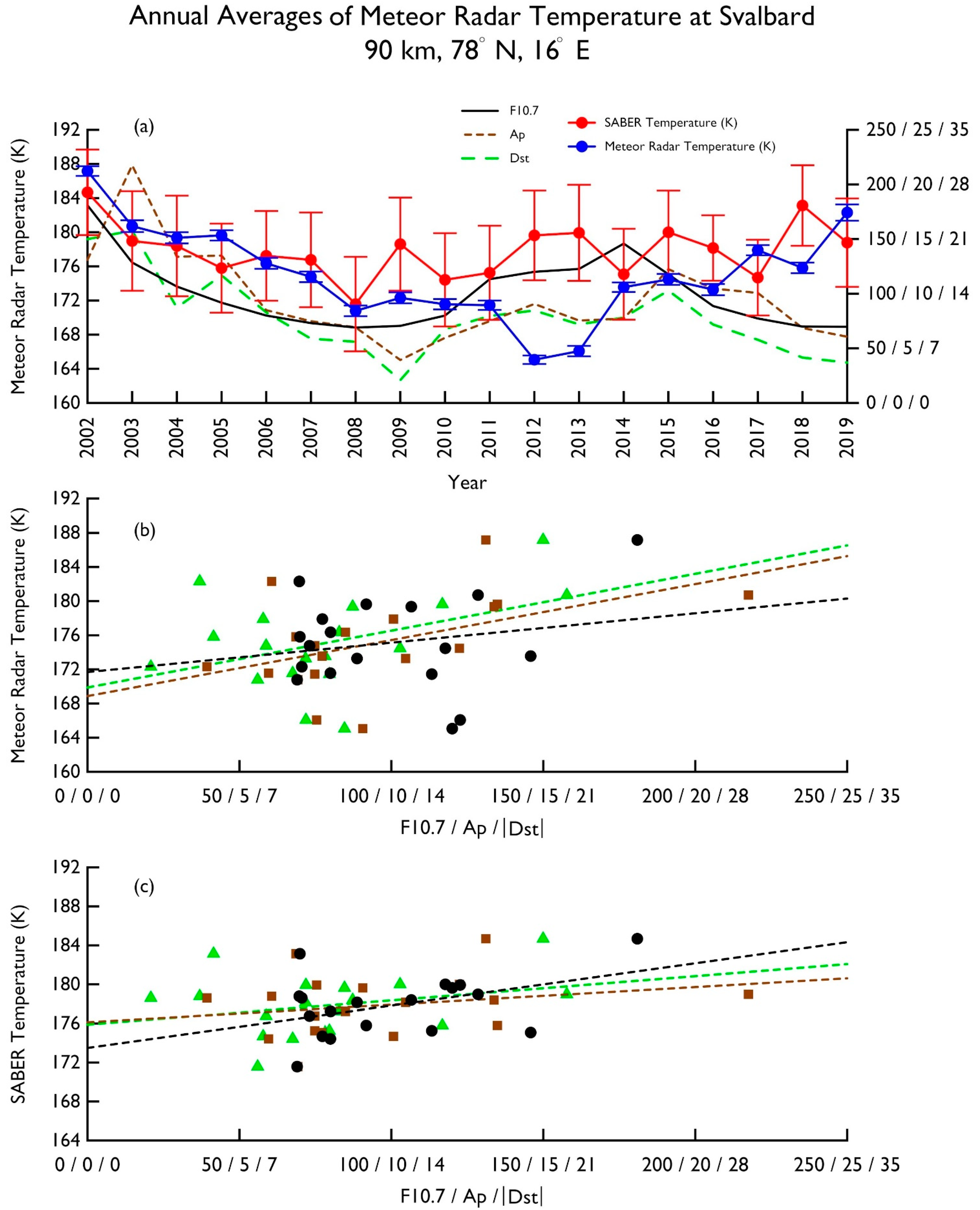
Here we first present the results of the ground-based and satellite measurements from the overlapped time period. The annual average of meteor radar temperature data at 90 km from Svalbard (axis on left, blue line with dots) and the annual average SABER temperature (axis on left, red line with dots) at the same altitude and location were plotted as a function of year from 2002 to 2019 as shown in Figure 1a. The error bars show the range of uncertainties for the temperatures. Also plotted in the figure are F10.7, Ap index, and |Dst| index (axis on right, black line for F10.7, brown dotted line for Ap index, and green dashed line for |Dst| index) as a function of year. Absolute values of Dst index were used in the plot for better visual inspection of its relation to Ap index. Examining the temperatures in Figure 1a, we can see that the SABER temperature at 90 km at the Svalbard location was warmer from 2006 to 2018, except for 2017, and was cooler prior to 2006 when compared to the Svalbard temperature. A large temperature difference of ~15 K was seen in 2012 and 2013. From the figure, we can see that both the SABER temperature and the Svalbard temperature showed a similar pattern to F10.7 from 2002 up until 2010; then, both datasets differed from the F10.7 pattern. As for Ap index and Dst index patterns, neither temperature dataset exhibited a strong resemblance to the patterns.
To find trends in the temperature data, we used the following equation:
where T(x) is the annual mean temperature; x is either F10.7, Ap index, or |Dst| index; A is the background temperature; and B is the trend. Svalbard and SABER temperatures from the same time period as a function of F10.7 (black dots), Ap index (brown squares), and |Dst| index (green triangles), as well as corresponding trend lines (black dashed line for F10.7 trend, brown dashed line for Ap index trend, and green dashed line for |Dst| trend), are shown in Figure 1b,c, respectively. The results are listed in Table 1. As we can see, the Svalbard (SABER) temperature had an F10.7 trend in the magnitude of 3.4 ± 4.3 K/100 SFU (4.3 ± 2.3 K/100 SFU) with a correlation coefficient, R = 0.2 (0.4). As for Ap index and |Dst| index trends, both were larger in the Svalbard temperatures (0.7 ± 0.3 K/nT, R = 0.5 for Ap and 0.5 ± 0.3 K/nT, R = 0.4 for |Dst|) with higher R values than in the SABER temperatures (0.2 ± 0.2 K/nT, R = 0.2 for Ap and 0.2 ± 0.2 K/nT, R = 0.3 for |Dst|).
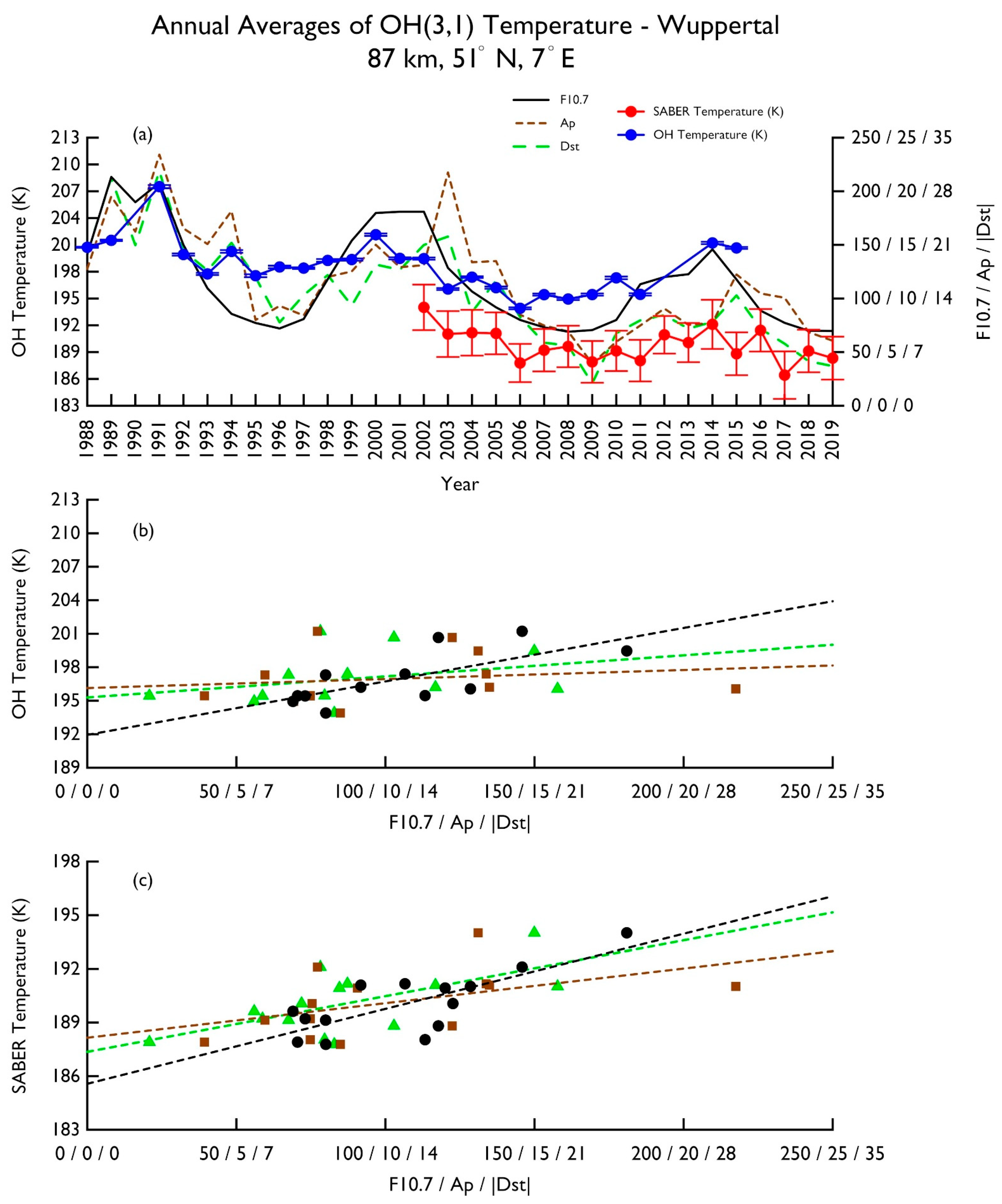
Figure 2a is similar to Figure 1a, but plotted with the annual averages of OH(3,1) airglow temperature data measured in Wuppertal (in blue line with dots) and the annual average SABER temperatures (in red line with dots) at 87 km at the same location. The overlapped period was from 2002 to 2015. As we can see, the overall pattern of WUP OH and that of SABER temperature looked similar, but the WUP OH temperature was consistently warmer than the SABER temperature throughout the overlapped time period. The temperature difference ranged from 5.0 to 11.8 K, with the largest temperature difference occurring in 2015. The temperatures, in general, followed the F10.7 variation. The linear regressions fit to both temperatures in F10.7 agreed with the visual inspection. The WUP and SABER temperatures from the same time period, with trend lines, are plotted in Figure 2b,c, respectively. The WUP OH (SABER) temperature showed an F10.7 trend of 4.7 ± 1.5 K/100 SFU (4.2 ± 1.0 K/100 SFU) with an R value of 0.7 (0.8). Both temperatures had similar F10.7 trends with the same level of correlation coefficient. When we compare the temperatures to the Ap index pattern, we can see that they overall looked similar to the Ap index variation between 2004 and 2014, but not so much outside of this time period. The linear regression of the WUP OH (SABER) temperature showed an Ap index trend of 0.1 ± 0.15 K/nT (0.2 ± 0.1 K/nT) with an R value of 0.2 (0.5). The linear-fit result indicated that the SABER temperature was moderately correlated with Ap index, whereas the WUP OH temperature was weakly correlated with Ap index. As for |Dst| index trend, it is not obvious to see in either temperature, but linear regression analysis showed a |Dst| index trend of 0.1 ± 0.1 K/nT with an R value of 0.3 in the WUP OH temperature and a trend of 0.2 ± 0.1 K/nT with a higher R value of 0.6 in the SABER temperature. Our trend analysis indicated that SABER temperature was more correlated with geomagnetic activity than the WUP OH temperature, judging from the R values for the Ap index and |Dst| index trends.
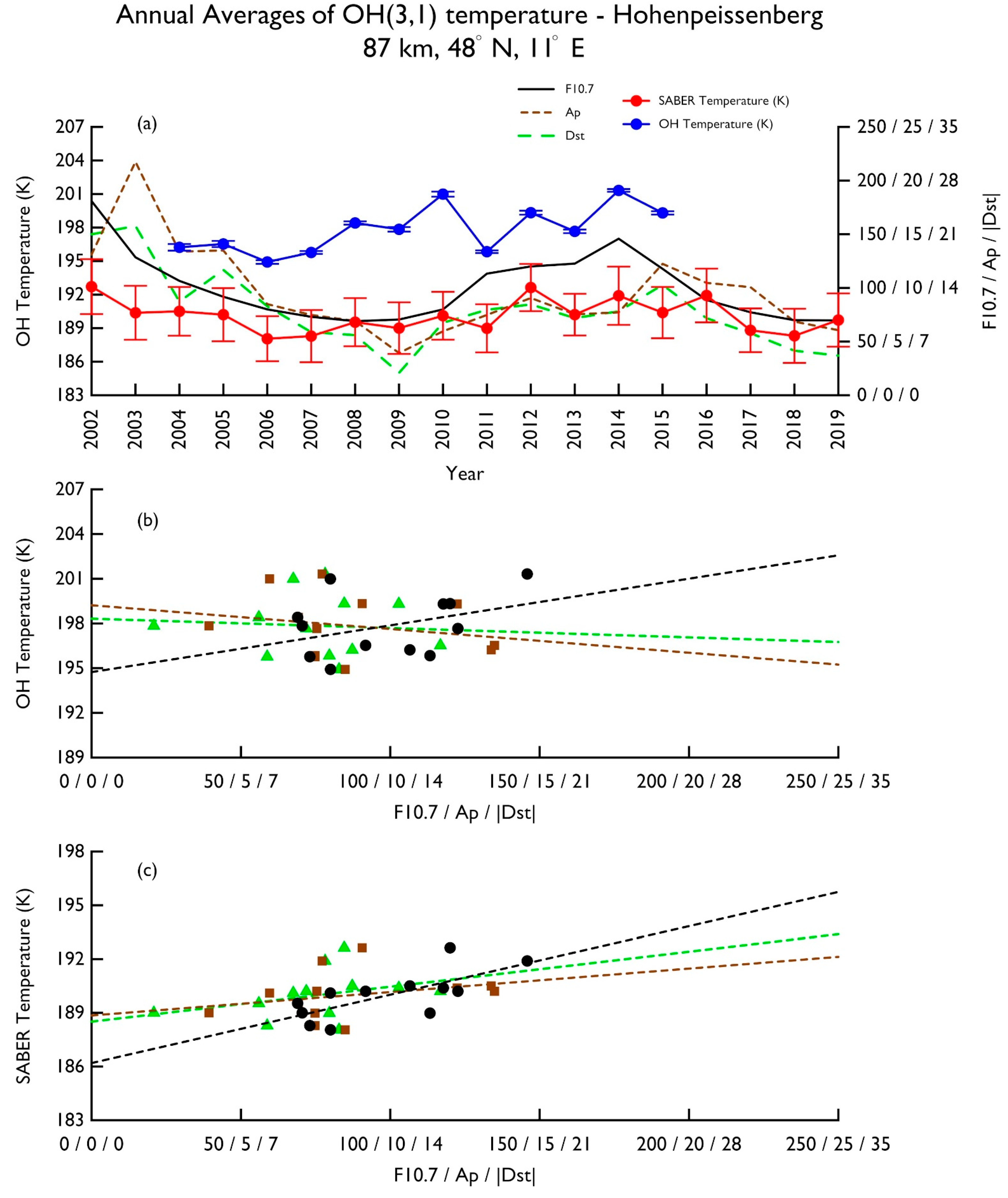
A similar plot using the annual averages of OH(3,1) temperature in Hohenpeissenberg and the SABER temperatures at the same location at 87 km is shown in Figure 3a. The overlapped time period was from 2004 to 2015. Like the WUP OH data, the HPB OH temperature data showed warmer temperatures than the SABER data, with a temperature difference ranging from 5.7 to 10.9 K. The largest temperature difference (10.9 K) was seen in 2010. Despite the temperature difference, both temperatures displayed very similar patterns, i.e., the peaks and troughs occurred in the same years. Both temperatures followed the F10.7 variation in general, except for 2010–2013. HPB and SABER temperatures with corresponding trend lines are shown in Figure 3b,c, respectively. Linear regression showed that the SABER temperature had an F10.7 trend of 3.8 ± 1.2 K/100 SFU with a moderately high R = 0.7, whereas the HPB OH temperature showed a trend of 3.2 ± 2.4 K/100 SFU with a lower correlation (R = 0.4). As for Ap index trend, both temperatures showed a low correlation. In addition, the HPB OH temperatures had a negative Ap index trend with a magnitude of −0.2 ± 0.2 K/nT (R = 0.2), and the SABER temperatures showed a positive Ap index trend of 0.1 ± 0.1 K/nT (R = 0.3). For |Dst| index trend, the SABER temperatures showed a trend of 0.1 ± 0.1 K/nT with a larger R = 0.4 and the HPB OH temperatures did not seem to display any |Dst| trend, as the trend value was an order of magnitude smaller, and the R value was very low with a value of ~0.1.
Since the length of time has been known to affect trend analysis results [4,17], we conducted another analysis of the WUP and HPB OH temperature data and the SABER temperature data at these two locations, but with the full range of available data. The results are displayed in Table 2. The most significant change was seen in the Ap and |Dst| index trends in the WUP OH temperature dataset. The Ap index trend value and the correlation coefficient went from ~0.1 K/nT, R = 0.2 to ~0.4 K/nT, R = 0.6. The |Dst| index trend and R values went from 0.1 K/nT, R = 0.3 to 0.3 K/nT, R = 0.7. The longer WUP dataset showed a slightly improved correlation with F10.7, but the trend value remained similar to that obtained from the shorter dataset. As shown in Table 2, the trend results using the longer WUP and SABER datasets compared better than the results using the data from the shorter time period. As for the SABER temperatures at the HPB location, the trend values did not change much, but the overall correlation was improved for all three trends when the longer dataset was used.
The linear trends reported in [12] are diverse, and most of them lack identification for their forcing. Instead of finding a linear trend directly from the dataset, we decided to use a different approach. It is known from simulation studies that an increase of CO2 gas concentration in the lower atmosphere leads to cooling in the upper atmosphere [6,7,18,19,20]. With a long-term record of CO2 gas emission data, the simulations in [7] showed that the temperature in the airglow altitudes would decrease at a rate of ~0.05 K/year in response to the increase of CO2 gas concentration. We reconducted the trend analysis, but with the influence of CO2 on temperature removed, i.e.,
where T’ is CO2-detrended temperature, T is the original temperature, y is year, and yi is the starting year in the data series. The temperature of the starting year was used as a reference, and here we used the full range of datasets for the analysis. The results, after detrending the CO2 influence, are displayed in Table 3. When we compare the detrending results to the nondetrending results (Svalbard location in Table 1 and WUP and HPB locations in Table 2), we can see that removing the CO2 influence on the temperature improved the correlation of temperature with F10.7, Ap, and |Dst|, and we obtained larger trends for all of the datasets except for the HPB OH temperature data, which did not show much improvement in the correlation with these influences even after the removal of CO2 influence.
4. Discussion
We should note that there exist inherent differences among the datasets because of the diverse geographic locations (78° N, 51° N, and 48° N) and the methods and assumptions used to derive the temperature data. Indeed, the derivation of OH temperature from relative intensities of different rotational lines of a rovibrational band is based on the assumption that the rotational population of the band is in local thermodynamic equilibrium (LTE) and the peak altitude is about 87 km [21]. However, neither assumption is always valid. The derivation of SABER temperature from CO2 emission at 15 μm [22] is sensitive to uncertainty in collisional rates when a non-LTE algorithm is used [23]. As for the derivation of meteor radar temperature, it is highly dependent on the model pressures used, and it has been found that temperatures derived under strong geomagnetic activity are erroneous [24]. These differences contributed to the different temperatures in the datasets.
The error associated with the NSMR meteor radar temperature measurements ranged from ~4 to 8%. The errors (uncertainties) of the WUP and HPB OH(3,1) temperature measurements were very small (see Figures 1 and 3 of [4]). The error in SABER temperature is estimated to be about 4 K (2%) in the 80–100 km altitude range [25]. Given that the errors/uncertainties were small, except for the meteor radar temperature under strong geomagnetic activity, they should not have affected the overall features of our trend results.
The ground-based temperature measurements, overlapped with the SABER temperature measurements at the three different locations, showed an F10.7 trend in the range of 3.2–4.7 K/100 SFU, with the WUP OH temperature showing the largest F10.7 trend value with a good correlation coefficient. The linear regression of Svalbard meteor radar temperatures in F10.7 had the smallest correlation coefficient. However, the Svalbard meteor radar temperature had the largest Ap index trend (~0.7 K/nT), whereas the HPB OH temperature showed a negative Ap index trend with a low correlation. The |Dst| index trend in these datasets showed similar behavior to that of the Ap index trends, i.e., the Svalbard meteor temperature was better correlated with |Dst| index than the OH temperature data, and the former had the largest |Dst| index trend. The HPB OH temperature had such a low correlation coefficient with |Dst| index that it could be considered as having no correlation.
Using the results of SABER temperatures from Table 1, we can see that SABER temperatures showed a good correlation with F10.7 at the WUP and HPB sites, but the correlation was lower at the Svalbard site. The F10.7 trend values were close to each other, in the range of 3.8–4.3 K/100 SFU. The SABER temperatures at the WUP site correlated better with Ap index than the temperatures measured at the other two sites, but the temperatures at all three locations showed similar Ap index trends of ~0.1–0.2 K/nT. As for |Dst| index trend, the SABER temperature at the WUP location had the largest trend value (0.2 K/nT) with the largest correlation coefficient (0.6), whereas the trend at the Svalbard and HPB locations were similar in terms of the trend value and correlation. We should note that in addition to the different geographic locations of the three sites, there is also a difference in altitude, which is 90 km for the Svalbard location and 87 km for the WUP and HPB locations. Having said that, the altitudinal difference of a few kilometers should not affect the results given the uncertainties and assumptions made in the temperature measurements.
The SABER temperatures at the Svalbard location showed a larger F10.7 trend and a higher correlation than the ground-based Svalbard measurements, but the ground-based measurements showed larger Ap and |Dst| index trends with better correlation than the satellite measurements. This might be because meteor radar temperature is more sensitive to geomagnetic activity. A study by Hall and Johnsen [24] using temperature results derived from two meteor radars found that temperature enhancements were very closely associated with enhancements in geomagnetic activity. Their study showed that “there is always a dependence of estimated temperature on geomagnetic activity of the order of 0.1–2.5 K/nT”. They attributed the geomagnetic activity-associated temperature enhancements to be erroneous. On the other hand, [26,27] indicated that geomagnetic activity produced temperature variations in the MLT region and that even weak geomagnetic activity can have an influence on the atmosphere. Additionally, our trend results from SABER or WUP temperatures and the simulation results in [7] also support the idea that the relationship between geomagnetic activity and temperature is positive and linear. These studies suggest that geomagnetic activity-associated temperature enhancements may be real. The SABER temperature trends at the WUP location compared well with the trends in the WUP ground-based measurements when the full range of datasets were used for the trend analysis. Both datasets showed an F10.7 trend in the 4.3–4.7 K/100 SFU range and an Ap (|Dst|) index trend in the 0.2–0.3 K/nT (0.2–0.3 K/nT) range. The full range of SABER temperatures at the HPB location and the HPB OH temperatures had similar F10.7 trends, ~3 K/100 SFU, but the latter showed a weak correlation. Both datasets showed weak correlations with Ap index, with the SABER temperatures displaying a positive trend of 0.1 K/nT and the HPB OH temperatures a negative trend of 0.2 K/nT.
While [28,29] suggested that a long-term trend study should be done separately for different seasons, and that “there is no physical sense to discuss a trend based on annual average temperatures” [28], we would argue otherwise. In order to minimize dynamical contribution from waves, seasonal variation, etc., the common procedure is to perform an average of the data on a timescale longer than the timescale of the variations. A prime example is the nightly average, where measurements in each night are averaged to minimize wave influence that has a time scale less than a few hours. Indeed, [8] showed that trends using zonal average annual mean SABER temperatures showed better correlation with F10.7 and Ap index than those using nonzonal annual mean SABER temperatures. The correlations were better primarily because the noise (planetary wave dynamics) was suppressed in the zonal average. Trend analysis using seasonal average data would inadvertently put more weight on the short-term dynamical contribution than appropriate for long-term trend studies. This is not to say that trends in seasonal average data are of no use, but rather they give a sense of the combined effect by short-term dynamical forcings and long-term influences. A proper way would be to use deseasonalized data to find trends by long-term influences when short-term dynamical forcings have been removed. Nevertheless, finding trends using seasonal average data was not germane to the focus and was beyond the scope of the current study. We would defer this investigation for a future study.
5. Conclusions
Annual averages of ground-based temperature measurements from Svalbard, Wuppertal, and Hohenpeissenberg were used to deduce F10.7, Ap index, and |Dst| index trends. The trends were then compared to the trends deduced from the annual averages of SABER temperature measurements from satellites at these locations. Meteor radar temperatures at 90 km at Svalbard from 2002 to 2019 showed a weak correlation with F10.7 and moderate correlations with Ap and |Dst| indices. The SABER temperatures from the same location, same height, and same time period showed a moderate correlation with F10.7 and weak correlations with Ap and |Dst| indices.
The OH(3,1) temperatures at Wuppertal at a nominal height of 87 km from 2002 to 2015 showed a good correlation with F10.7 and weak correlations with Ap and |Dst| indices, whereas the SABER temperatures from the same time period showed a good correlation with F10.7 and moderate-to-good correlations with Ap and |Dst| indices. When we used a full range of available datasets, 1988 to 2015 for Wuppertal and 2002 to 2019 for SABER, it was found that the Wuppertal temperature showed a much better correlation with Ap and |Dst| indices and that the trend values were closer to those obtained from the SABER temperature measurements.
The OH(3,1) temperature at Hohenpeissenberg from 2004 to 2015 showed weak correlations with F10.7 and Ap index and no correlation with |Dst| index. SABER temperatures, from the same time period or from 2002 to 2019, and the OH(3,1) temperature at Hohenpeissenberg all showed similar F10.7 trends, but SABER temperature showed a good correlation with F10.7 while the Hohenpeissenberg temperature showed a moderate correlation. The datasets showed rather weak correlations with Ap index, with the Hohenpeissenberg data showing a decreasing trend.
Given that CO2 gas emission has been increasing steadily over the past few decades, the cooling in the MLT region due to the CO2 increase should be taken into account in the trend analysis. Therefore, we also performed a trend analysis of the CO2-detrended data over the full range, using a cooling rate of 0.05 K/y. We found that most of the detrended temperatures overall showed slightly better correlations with F10.7, Ap index, and |Dst| index, and the trend values became slightly larger. Also, the ground-based data and SABER data from the same time period were analyzed to see if it would close the gap between the trend results from these datasets when the time period of the data was not a variant. We found that using the data from a short overlapped time period did not necessarily close the gap for all the datasets considered in this study. Our study clearly shows that a longer dataset would be better to capture the trends in the temperature, as was evidenced by the results for the Wuppertal data.
Author Contributions
Conceptualization, T.-Y.H.; Formal analysis, T.-Y.H. and M.V.; Funding acquisition, T.-Y.H.; Investigation, T.-Y.H. and M.V.; Methodology, T.-Y.H.; Project administration, T.-Y.H.; Resources, T.-Y.H.; Software, M.V.; Writing—original draft, T.-Y.H. All authors have read and agreed to the published version of the manuscript.
Funding
This research was funded by US NSF AGS-1903346 to The Pennsylvania State University.
Institutional Review Board Statement
Not applicable.
Informed Consent Statement
Not applicable.
Data Availability Statement
Data used for this study can be found here, https://pennstateoffice365-my.sharepoint.com/:f:/g/personal/tuh4_psu_edu/EheClDKG0xZIvQ4vK_a-QA8BsXYWERJ41ksWzMc4gOSqUA?e=jhlTSu, accessed on 12 August 2021.
Acknowledgments
T.-Y. Huang and M. Vanyo acknowledge support from the US NSF AGS-1903346 to Pennsylvania State University. We greatly appreciate Chris Hall for providing the meteor radar temperature at Svalbard and Christoph Kalicinsky for providing the OH* temperature data measured at Wuppertal and Hohenpeissenberg. SABER temperature level 2 data was downloaded from http://saber.gats-inc.com/ (accessed on 20 February 2021). F10.7 values were obtained from the NASA website (http://omniweb.gsfc.nasa.gov/form/dx1.html, accessed on 20 November 2020). Ap index and Dst index values were obtained from the World Data Center for Geomagnetism, Kyoto website (http://wdc.kugi.kyoto-u.ac.jp/, accessed on 4 March 2021).
Conflicts of Interest
The authors declare no conflict of interest. The funders had no role in the design of the study; in the collection, analyses, or interpretation of data; in the writing of the manuscript, or in the decision to publish results.
References
- Espy, P.J.; Stegman, J. Trends and variability of mesospheric temperature in high-latitudes. Phys. Chem. Earth 2002, 27, 543–553. [Google Scholar] [CrossRef]
- Offermann, D.; Hoffmann, P.; Knieling, P.; Koppmann, R.; Oberheide, J.; Steinbrecht, W. Long-term trend and solar cycle variations of mesospheric temperature and dynamics. J. Geophys. Res. 2010, 115, D18127. [Google Scholar] [CrossRef]
- Hall, C.M.; Dyrland, M.E.; Tsutsumi, M.; Mulligan, F.J. Temperature trends at 90 km over Svalbard, Norway (78° N 16° E), seen in one decade of meteor radar observations. J. Geophys. Res. 2012, 117, D08104. [Google Scholar] [CrossRef]
- Kalicinsky, C.; Knieling, P.; Koppmann, R.; Offermann, D.; Steinbrecht, W.; Wintel, J. Long-term dynamics of OH* temperatures over central europe: Trends and solar correlations. Atmos. Chem. Phys. 2016, 16, 15033–15047. [Google Scholar] [CrossRef] [Green Version]
- Perminov, V.I.; Semenov, A.I.; Pertsev, N.N.; Medvedeva, I.V.; Dalin, P.A.; Sukhodoev, V.A. Multi-year behavior of the midnight OH* temperature according to observations at Zvenigorod over 2000–2016. Adv. Space Res. 2018, 61, 1901–1908. [Google Scholar] [CrossRef]
- Huang, T.-Y. Influences of CO2 increase, solar cycle variation, and geomagnetic activity on airglow from 1960 to 2015. J. Atmos. Solar Terr. Phys. 2018, 171, 164–175. [Google Scholar] [CrossRef]
- Huang, T.-Y.; Vanyo, M. Trends in the airglow temperatures in the MLT region—Part 1: Model simulations. Atmosphere 2020, 11, 468. [Google Scholar] [CrossRef]
- Huang, T.-Y.; Vanyo, M. Trends in the airglow temperatures in the MLT region—Part 2: SABER observations and comparisons to model simulations. Atmosphere 2021, 12, 167. [Google Scholar] [CrossRef]
- Yuan, T.; Solomon, S.C.; She, C.-Y.; Krueger, D.A.; Liu, H.-L. The long-term trends of nocturnal mesopause temperature and altitude revealed by Na lidar observations between 1990 and 2018 at midlatitude. J. Geophys. Res. Atmos. 2019, 124, 5970–5980. [Google Scholar] [CrossRef] [Green Version]
- She, C.-Y.; Berger, U.; Yan, Z.-A.; Yuan, T.; Lübken, F.-J.; Krueger, D.A.; Hu, X. Solar response and long-term trend of midlatitude mesopause region temperature based on 28 years (1990–2017) of Na lidar observations. J. Geophys. Res. Space Phys. 2019, 124, 7140–7156. [Google Scholar] [CrossRef]
- Beig, G. Long-term trends in the temperature of mesosphere/lower thermosphere region: 2. solar response. J. Geophys. Res. 2011, 116, A00H12. [Google Scholar] [CrossRef]
- Beig, G. Long-term trends in the temperature of mesosphere/lower thermosphere region: 1. anthropogenic influences. J. Geophys. Res. 2011, 116, A00H11. [Google Scholar] [CrossRef] [Green Version]
- Huang, T.-Y.; Hickey, M.P. On the latitudinal variations of the non-periodic response of minor species induced by a dissipative gravity-wave packet in the MLT region. J. Atmos. Solar Terr. Phys. 2007, 69, 741–757. [Google Scholar] [CrossRef]
- Huang, T.-Y.; Hickey, M.P. Secular variations of OH nightglow emission and of the OH intensity-weighted temperature induced by gravity-wave forcing in the MLT region. Adv. Space Res. 2008, 41, 1478–1487. [Google Scholar] [CrossRef]
- Huang, T.-Y.; George, R. Simulations of gravity wave-induced variations of the OH(8,3), O2(0,1), and O(1S) airglow emissions in the MLT region. J. Geophys. Res. Space Phys. 2014, 119, 2149–2159. [Google Scholar] [CrossRef]
- Amaro-Rivera, Y.; Huang, T.-Y.; Urbina, J.; Vargas, F. Empirical values of branching ratios in the three-body recombination reaction for O(1S) and O2(0,0) airglow chemistry. Adv. Space Res. 2018, 62, 2679–2691. [Google Scholar] [CrossRef]
- Huang, T.-Y.; Kane, T.J. Examining methods used in extracting long-term thermospheric density trends. J. Atmos. Solar Terr. Phys. 2013, 97, 115. [Google Scholar] [CrossRef]
- Roble, R.G.; Dickinson, E.E. How will changes in carbon dioxide and methane modify the mean structure of the mesosphere and thermosphere? Geophys. Res. Lett. 1989, 16, 1441–1444. [Google Scholar] [CrossRef] [Green Version]
- Huang, T.-Y. Global warming’s effect on mesospheric airglow emissions. In New Developments in Global Warming Research; Keyes, C.B., Lucero, O.C., Eds.; Nova Science Publishers Inc.: New York, NY, USA, 2013; pp. 103–116. [Google Scholar]
- Huang, T.-Y. Simulations of airglow variations induced by the CO2 increase and solar cycle variation from 1980 to 1991. J. Atmos. Solar Terr. Phys. 2016, 147, 138–147. [Google Scholar] [CrossRef] [Green Version]
- Von Savigny, C. Airglow in the earth atmosphere: Basic characteristics and excitation mechanisms. ChemTexts 2017, 3, 1–9. [Google Scholar] [CrossRef]
- Mertens, C.J.; Mlynczak, M.G.; López-Puertas, M.; Wintersteiner, P.P.; Picard, R.H.; Winick, J.R.; Gordley, L.L.; Russell, J.M. Retrieval of mesospheric and lower thermospheric kinetic temperature from measurements of CO2 15 μm Earth Limb Emission under non-LTE conditions. Geophys. Res. Lett. 2001, 28, 1391–1394. [Google Scholar] [CrossRef]
- García-Comas, M.; López-Puertas, M.; Marshall, B.T.; Wintersteiner, P.P.; Funke, B.; Bermejo-Pantaleón, D.; Mertens, C.J.; Remsberg, E.E.; Gordley, L.L.; Mlynczak, M.G.; et al. Errors in sounding of the atmosphere using broadband emission radiometry (SABER) kinetic temperature caused by non-local-thermodynamic-equilibrium model parameters. J. Geophys. Res. 2008, 113, D24106. [Google Scholar] [CrossRef] [Green Version]
- Hall, C.M.; Johnsen, M.G. Influence of geomagnetic activity on derivation of temperatures from meteor wind radars. Radio Sci. 2020, 55, e2020RS007123. [Google Scholar] [CrossRef]
- Xu, J.; She, C.Y.; Yuan, W.; Mertens, C.; Mlynczak, M.; Russell, J. Comparison between the temperature measurements by TIMED/SABER and lidar in the midlatitude. J. Geophys. Res. 2006, 111, A10S09. [Google Scholar] [CrossRef]
- Wang, N.; Yue, J.; Wang, W.; Qian, L.; Jian, L.; Zhang, J. A comparison of the CIR- and CME-induced geomagnetic activity effects on mesosphere and lower thermospheric temperature. J. Geophys. Res. Space Phys. 2021, 126, e2020JA029029. [Google Scholar] [CrossRef]
- Cai, X.; Burns, A.G.; Wang, W.; Qian, L.; Solomon, S.C.; Eastes, R.W.; Pedatella, N.; Daniell, R.E.; McClintock, W.E. The two-dimensional evolution of thermospheric ∑O/N2 response to weak geomagnetic activity during solar-minimum observed by GOLD. Geophys. Res. Lett. 2020, 47, e2020GL088838. [Google Scholar] [CrossRef]
- Dalin, P.; Perminov, V.; Pertsev, N.; Romejko, V. Updated long-term trends in mesopause temperature, airglow emissions, and noctilucent clouds. J. Geophys. Res. Atmos. 2020, 125, e2019JD030814. [Google Scholar] [CrossRef]
- Grygalashvyly, M.; Sonnemann, G.R.; Lübken, F.-J.; Hartogh, P.; Berger, U. Hydroxyl layer: Mean state and trends at midlatitudes. J. Geophys. Res. Atmos. 2014, 119, 12391–12419. [Google Scholar] [CrossRef]
Figure 1.
(a) Annual averages of meteor radar temperatures at Svalbard (blue line with dots) and annual averages of SABER temperatures (red line with dots) at the same location at 90 km altitude. The error bars show the range of uncertainties for the temperatures. Also plotted are annual averages for F10.7 (black line), Ap index (brown dashed line), and |Dst| index (green dashed line). (b) Svalbard temperatures plotted as a function of F10.7 (in black), Ap index (in brown), and |Dst| index (in green) with the respective trend lines. (c) SABER temperatures plotted as a function of F10.7, Ap index, and |Dst| index with the respective trend lines.

Figure 2.
(a) Annual averages of OH(3,1) temperatures at Wuppertal (blue line with dots) and annual averages of SABER temperatures (red line with dots) at the same location at 87 km altitude. The error bars show the range of uncertainties of temperature. Also plotted are annual averages of F10.7 (black line), Ap index (brown dashed line), and |Dst| index (green dashed line). (b) WUP temperatures plotted as a function of F10.7 (in black), Ap index (in brown), and |Dst| index (in green) with the respective trend lines. (c) SABER temperatures plotted as a function of F10.7, Ap index, and |Dst| index with the respective trend lines.

Figure 3.
(a) Annual averages of OH(3,1) temperatures at Hohenpeissenberg (blue line with dots) and annual averages of SABER temperatures (red line with dots) at the same location at 87 km altitude. The error bars show the range of uncertainties of temperature. Also plotted are annual averages of F10.7 (black line), Ap index (brown dashed line), and |Dst| index (green dashed line). (b) HPB temperatures plotted as a function of F10.7 (in black), Ap index (in brown), and |Dst| index (in green) with the respective trend lines. (c) SABER temperatures plotted as a function of F10.7, Ap index, and |Dst| index with the respective trend lines.


Table 1.
Trends with correlation coefficient R obtained from ground-based and SABER temperature measurements from the overlapped time period.
Table 1.
Trends with correlation coefficient R obtained from ground-based and SABER temperature measurements from the overlapped time period.
| Trends | R | Trends | R |
|---|---|---|---|
| Svalbard, 2002–2019 | SABER at 90 km | ||
| 0.2 | 0.4 | ||
| 0.5 | 0.2 | ||
| 0.4 | 0.3 | ||
| Wuppertal, 2002–2015 | SABER at 87 km | ||
| 0.7 | 0.8 | ||
| 0.2 | 0.5 | ||
| 0.3 | 0.6 | ||
| Hohenpeissenberg, 2004–2015 | SABER at 87 km | ||
| 0.4 | 0.7 | ||
| 0.2 | 0.3 | ||
| 0.1 | 0.4 | ||
Table 2.
Trends with correlation coefficient R obtained using the full ranges of ground-based and SABER temperature measurements.
Table 2.
Trends with correlation coefficient R obtained using the full ranges of ground-based and SABER temperature measurements.
| Trends | R | Trends | R |
|---|---|---|---|
| Wuppertal, 1988–2015 | SABER, 2002–2019 at 87 km | ||
| 0.7 | 0.7 | ||
| 0.6 | 0.5 | ||
| 0.7 | 0.6 | ||
| Hohenpeissenberg, 2004–2015 | SABER, 2002–2019 at 87 km | ||
| 0.4 | 0.7 | ||
| 0.2 | 0.3 | ||
| 0.1 | 0.5 | ||
Table 3.
Trends with correlation coefficient R after a cooling trend of 0.05 K/y was removed from the datasets.
Table 3.
Trends with correlation coefficient R after a cooling trend of 0.05 K/y was removed from the datasets.
| Trends | R | Trends | R |
|---|---|---|---|
| Svalbard | SABER at 90 km | ||
| 0.2 | 0.5 | ||
| 0.5 | 0.3 | ||
| 0.5 | 0.3 | ||
| Wuppertal | SABER at 87 km | ||
| 0.7 | 0.7 | ||
| 0.6 | 0.5 | ||
| 0.7 | 0.7 | ||
| Hohenpeissenberg | SABER at 87 km | ||
| 0.3 | 0.8 | ||
| 0.2 | 0.4 | ||
| 0.1 | 0.6 | ||
Publisher’s Note: MDPI stays neutral with regard to jurisdictional claims in published maps and institutional affiliations. |
© 2021 by the authors. Licensee MDPI, Basel, Switzerland. This article is an open access article distributed under the terms and conditions of the Creative Commons Attribution (CC BY) license (https://creativecommons.org/licenses/by/4.0/).
Share and Cite
MDPI and ACS Style
Huang, T.-Y.; Vanyo, M. Trends in the Airglow Temperatures in the MLT Region—Part 3: Ground-Based and SABER Measurements. Atmosphere 2021, 12, 1161. https://0-doi-org.brum.beds.ac.uk/10.3390/atmos12091161
AMA Style
Huang T-Y, Vanyo M. Trends in the Airglow Temperatures in the MLT Region—Part 3: Ground-Based and SABER Measurements. Atmosphere. 2021; 12(9):1161. https://0-doi-org.brum.beds.ac.uk/10.3390/atmos12091161
Chicago/Turabian StyleHuang, Tai-Yin, and Michael Vanyo. 2021. "Trends in the Airglow Temperatures in the MLT Region—Part 3: Ground-Based and SABER Measurements" Atmosphere 12, no. 9: 1161. https://0-doi-org.brum.beds.ac.uk/10.3390/atmos12091161
Note that from the first issue of 2016, this journal uses article numbers instead of page numbers. See further details here.