Relationships between Vertical Temperature Gradients and PM₁₀ Concentrations during Selected Weather Conditions in Upper Silesia (Southern Poland)

Abstract

This paper studies surface air temperature inversions and their impact on air pollution under the background of meteorological conditions in southern Poland. The relationship of temperature gradients and air quality classes with weather conditions in the most urbanized and polluted part of Poland as represented by the Upper Silesia region (USR) within the administrative boundaries of the Górnośląsko-Zagłębiowska Metropolis (GZM) is presented. Based on probability analysis this study hierarchized the role of the selected weather elements in the development of surface-based temperature inversion (SBI) and air quality (AQ). The thresholds of weather elements for a rapid increase in the probability of oppressive air pollution episodes were distinguished. Although most SBI occurred in summer winter SBIs were of great importance. In that season a bad air quality occurred during >70% of strong inversions and >50% of moderate inversions. Air temperature more strongly triggered AQ than SBI development. Wind speed was critical for SBI and significant for AQ development. A low cloudiness favored SBI occurrence altered air quality in winter and spring during SBI and favored very bad AQ5 (>180 µg/m³) occurrence. The probability of high air pollution enhanced by SBI rapidly increased in winter when the air temperature dropped below −6 °C the wind speed decreased below 1.5 m/s and the sky was cloudless. Changes in the relative humidity did not induce rapid changes in the occurrence of bad AQ events during SBI

1. Introduction

Vertical air temperature profile is critical for determining the height of the planetary boundary layer [1] and the state of the atmosphere [2,3,4,5]. A negative vertical gradient <−0.98 K/100 m (dry adiabatic lapse rate) indicates an unstable air column, while an inverted situation in which warm air overlies cooler air is characteristic of temperature inversion [6,7]. The formation of surface-based temperature inversions (SBIs) is triggered by longwave radiative cooling at the surface [5,6,8,9,10]. Such a mechanism operates at night under little or no cloud cover and light or calm wind conditions [6]. After sunrise, the surface of the Earth absorbs solar radiation, and the air above the surface becomes unstable [5]. SBIs largely control the vertical movement of pollution; therefore, studying the occurrence of SBIs that can cause oppressive and health-threatening episodes of high air pollution concentrations in urban areas is particularly important [11,12,13,14,15,16].

In the Upper Silesia Region, episodes of high air pollutant concentrations are very common during the cold season. For example, during an SBI with an intensity of 8 K/100 m that took place over GZM (Southern Poland) on 8 February 2015, the maximum hourly concentrations of PM₁₀ and SO₂ were 414 μg/m³ and 189 μg/m³, respectively. An even more drastic episode was recorded on 9 January 2017, during a high-pressure wedge and polar continental air masses over the region. Frost prevailed that day with air temperature of −19.2 °C. During the night, the air temperature inversion was as strong as 8.1 K/100 m, resulting in extremely high concentrations of pollutants. According to the Voivodship Inspectorate of Environmental Protection, the PM₁₀ concentration was 985 μg/m³ in Dąbrowa Górnicza (11 pm) and 667 μg/m³ in Katowice (4 am).

In addition, SBI plays an important role in regulating turbulent flux regimes in ecosystems and the surface energy balance [17,18,19] and co-occurs with meteorological phenomena that affect the quality of human life. These phenomena include the formation of fog and ground frost, which disrupt the activities of the transportation and agriculture industries [7,20,21,22].

The frequency and persistence of SBI exhibits geographic variations depending on the climate, topography, and weather of an area. In polar climates, SBI is the most characteristic and periodically persistent feature of the atmospheric boundary layer e.g., [8,10,23,24,25,26,27,28,29,30,31]. At high latitudes under long and severe winters, short days are not long enough to allow radiation to dissipate SBI [6,31,32,33]. Permanent inversions have been found over the Antarctic Plateau in winter [31]. In midwinter, SBI can persist for several days in basins and valleys [9,34]. All-day or diurnal SBI is also possible at other locations due to their specific synoptic conditions, including the advection of warm air masses [33,35]. Adiabatic compression of air in anticyclonic systems [20,36,37,38,39] leads to the formation of elevated inversions [33,35,40], but these conditions fall outside the scope of this paper. Anticyclonic conditions also lead to an increased SBI strength and thickness due to reductions in cloud cover, as can be seen in Greenland [41]. However, in Central Europe most SBI occurs during nights in summer season [42,43,44,45,46,47].

Meteorological factors known to control the build-up or strengthening of SBI at various locations include low wind speeds [31,32,48,49,50], snow-covered surfaces that plunge air temperature and reflect solar radiation [51], and sea breezes [52]. Conversely, Milionis and Davies [53] identified no association between temperature inversions and local wind maximums and vertical wind shear actions. Urban and topographic complexities may modify the formation and disruption of SBI, supporting the need for local studies of vertical air temperature profiles [1]. In urban areas in Japan, no inversion is observed in winter due to heat supply originating from the seas and strong winds near the coast [54]. A lower frequency of nocturnal SBI in urban environments relative to suburban areas was also found in Krakow [42] and Moscow [55].

Surface-based air temperature inversions are of great importance to enhance air pollutant concentrations, particularly in winter [5,10,29,35,50,56,57,58,59,60]. Air pollution similarly to SBI, reveals a close relationship with weather conditions, including air temperature, relative humidity, wind speed, solar radiation, and pressure [50,61,62,63]. Various wind speed thresholds dictating air pollutant concentrations are mentioned in the literature, e.g., <4 m/s¹ [64] or <3 m/s¹ [65]. Low wind speeds were found to favor the accumulation of industrial emissions [50,66,67,68,69,70,71].

A strong linkage was found between the concentration of air pollutants and both mesoscale [35,62,72,73] and large-scale atmospheric circulation [74]. The influence of air mass advection on air pollution was also studied using backward trajectories [68,73,75]. In Upper Silesia during the period 1994–2004 [76], under anticyclonic conditions the pollutant concentrations reach two to three times the permissible level of 50 µg/m³, particularly in autumn, winter and early spring.

The above literature overview revealed that both SBI and air pollution depend on meteorological conditions; however, a complex study of co-occurring phenomena (SBI and AQ) under the background weather conditions described by selected meteorological elements has not been studied based on long-term vertical measurements (25 years) in an urban environment. The vast majority of studies have used data from short-term experiments, ranging from several months to 5 years e.g., [77,78,79,80], or from weather stations located at the ground surface but at various altitudes e.g., [1,53,57]. Complex studies counting a set of meteorological elements and their impacts on SBI and air pollution are rare [39,56,81]. The data used in this study are important because vertical meteorological measurements collected in cities/urban environments are rare. According to Wolf et al. [78], in situ measurements of temperature profiles at elevations a few tens or hundreds of meters above the ground are difficult and costly, if not impossible, in urbanized areas. In Poland, only three radiosonde stations, located outside the cities, are in operation, and none of them are located in the Upper Silesia region. Moreover, soundings are performed twice a day at 00 and 12 UTC. According to radiosounding in Wrocław (SW Poland) during the period 2001–2020, the average depth of the SBI layer at night is 207 m, changing from 186 m in spring to 249 m in winter. Most often (81%), the SBI thickness ranges from 50 to 300 m [47,60].

This study discusses the complex relationships between air temperature gradients in the near-ground troposphere and air quality based on PM₁₀ concentrations and weather conditions. The calculated mean values of selected meteorological elements for unstable and stable atmospheres and conditional probabilities for defined ranges of meteorological elements also allowed hierarchization of the role that meteorological elements play in SBI development and AQ. The novelty of this study includes the long-term (19 years) series of air temperature gradients of high temporal resolution (10 min) and the results on annual and diurnal courses of the thermal structure of the atmosphere focusing on ground-level inversions in the typical urban and industrial area of the Upper Silesia. The comprehensive impact of the thermal gradients in combination with weather conditions (wind, cloud cover, air humidity) on the atmospheric pollution has not been studied so far in the Górnośląsko-Zagłębiowska Metropolis. The results of this study help us understand the distribution of air pollution and may be useful for authorities to mitigate the negative impacts of bad air quality, prediction and modelling studies on surface-based air temperature inversion, and air quality in urban areas located on uplands in temperate climate zones. The introduction is outlined in Section 1, and the data and methods are described in Section 2. The daily and annual courses of air temperature gradients and air quality classes are discussed in Section 3 and Section 4, respectively. The relationships between air pollution (concentration of PM₁₀) and various air temperature gradients are discussed in Section 5. Section 6 characterizes the weather conditions described by air temperature, wind speed, cloudiness, and relative humidity under strong and conditionally unstable (γ < −0.5 K/100 m) and stable (γ > 1 K/100 m) conditions and dependently on AQ. The probability of ground-based SBI and bad or very bad air quality classes depending on the ranges of various meteorological elements are presented in Section 7. Section 8 and Section 9 provide the discussion and conclusions, respectively.

2. Research Area, Data, and Methods

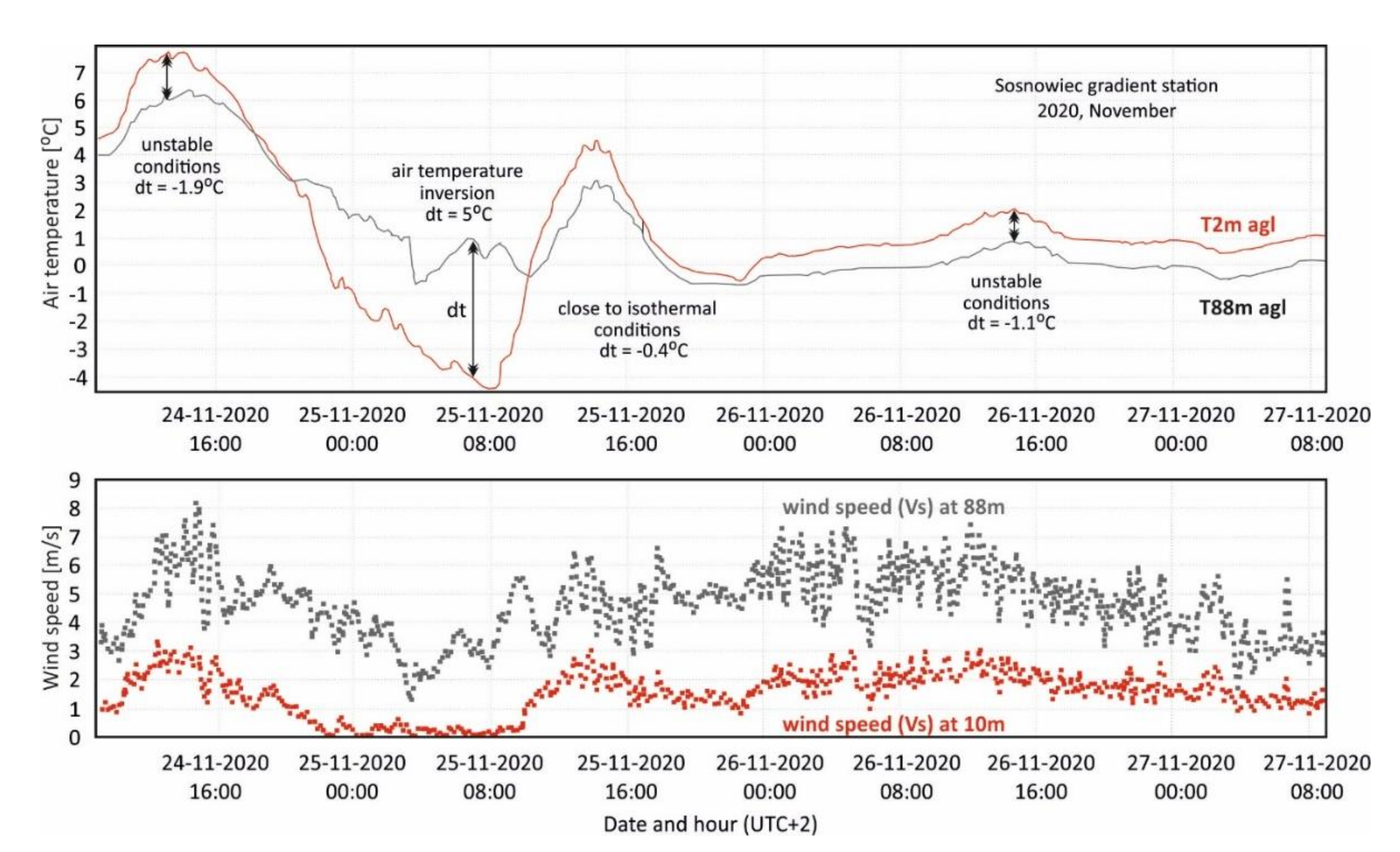
2.1. Research Area and Data

The Górnośląsko-Zagłębiowska Metropolis (GZM) is located in the central part of southern Poland (Figure 1) and is the most urbanised part of the country and most polluted part of Europe. The GZM occupies an area of 2553 km² and is inhabited by almost 2.3 million people. The daily threshold for the mass concentration of PM₁₀ (>50 μg/m³) is exceeded considerably during the heating season in all metropolis cities [82]. The main source of air pollution near the ground atmosphere level below 50 m is the emission domestic premises during the cold season and the road transport across the whole year. The emission from mining and metallurgical industries emission takes place all year round to slightly higher layers of the atmosphere about 100–150 m above the ground [76,83,84].

The meteorological gradient station that collected the measurements in the vertical profile of the lower troposphere is located in the central part of the GZM area at the Institute of Earth Sciences in Sosnowiec, the University of Silesia in Katowice (50°17′ N, 19°08′ E, 263 m above sea level, Figure 1). The measurements are performed at the ground meteorological station and on the roof of the Institute of Earth Sciences building at a height of 88 m above the ground in line with the WMO standards. The gradient station delivers unique, long-term (1993–until now), and high-temporal-resolution (10 min) meteorological data from the center of an urbanized area. Temperature sensors were recalibrated every time they were replaced and after any station failures. The accuracy of temperature measurements is about ±0.2 °C. The comparison of air temperature measured at the two levels for selected days representing various weather conditions presented no signs that the roof impacts the quality of measurements, as the sensors were located about 5 m above the roof surface. During clear nights with low wind speeds, the gradient was positive, indicating the occurrence of air temperature inversions, while on cloudy days with higher wind speeds, the temperature gradient (γ) was negative and varied at approximately −1 °C per 100 m (Figure 2). The data we possess do not provide information regarding surface-based temperature inversion depths, but they do enable the study of the daily course of SBI frequency and intensity and its detailed relation to weather conditions.

The development and dissipation of SBI are closely related to weather conditions and immediately respond to changes or variability in some meteorological elements (particularly to wind speed). Therefore, we used 1-h-resolution data for both the meteorological elements and PM₁₀ concentrations. The primary meteorological data used in this study include the hourly averages of air temperature, wind speed and relative humidity (calculated from 10 min data). The cloudiness data were taken from the Katowice Muchowiec Airport synoptic station of the Institute of Meteorology and Water Management (9 km to SW from gradient stations) because visual observations at the gradient station are performed occasionally. The existing cloudiness observations from the gradient station were compared with data from Katowice Muchowiec and showed a great degree of agreement.

To assess the impact of SBI on air quality, we also used the particulate matter concentration (PM₁₀) data from 4 monitoring stations operating within the Silesian Air Monitoring of the Regional Inspectorate of Environmental Protection, which is freely available from the webpage of http://powietrze.katowice.wios.gov.pl/ (accessed 21 January 2021). The monitoring stations representing the most heavily inhabited central parts of the GZM area and the Silesian voivodeship (Figure 1) are located at distances of 2 km (Sosnowiec), 14 km (Katowice), 25 km (Zabrze) and 32 km (Gliwice) from the gradient stations. The average values of PM₁₀ concentration at these 4 stations well represent the aero-sanitary conditions of the entire Silesia region. Correlation coefficients between the average monthly PM₁₀ at individual stations and the area average in the period 1994–2020 ranged from 0.92 to 0.96.

List of variables used in this paper are presented in

Table 1. List of meteorological variables (hourly values).

Symbol	Variable (Unit)
AT2; T2	Air temperature 2 m (°C)
AT88; T88	Air temperature 88 m (°C)
dt	Temperature difference: dt = AT88 − AT2 (K)
γ; ATG	Vertical temperature gradient: γ = (AT88 − AT2)/86 ∗ 100 (K/100 m)
PM10	Particulate matter of less than 10 microns (μg/m3)
V	Wind speed (m/s)
N	Cloudiness (% of sky coverage; N% = N octas * 12.5)
N ≤ 20%	Clear hours
N ≥ 80%	Cloudy hours
RH	Relative humidity (%)
RH < 50%	Dry hours
RH > 80%	Wet hours

. The data are not complete. Gaps in data result from the breaking of measurement tools or energy failures (

Table 2. Characteristic of hourly data completeness expressed as a percentage of seasons [%] with: ND—no data, Full—complete data, G ≤ 20%—gaps covering ≤20% of hours, G > 20%—gaps covering >20% of hours for selected meteorological elements and air monitoring stations in 1993–2020.

Season		AT2	AT88	dt	V	PM10S	PM10K	PM10Z	PM10G
MAM	ND	12	12	12	4	16	2	2	10
	Full	75	75	76	82	36	46	70	63
	G ≤ 20%	80	80	80	92	81	94	88	86
	G > 20%	8	8	8	5	4	4	10	5
JJA	ND	7	7	7	9	20	6	2	12
	Full	65	65	67	68	36	44	58	58
	G ≤ 20%	78	78	78	88	73	88	90	78
	G > 20%	6	6	6	5	7	6	7	10
SON	ND	15	15	15	14	16	4	10	8
	Full	68	68	70	71	45	61	54	60
	G ≤ 20%	76	76	76	78	78	90	84	86
	G > 20%	9	9	9	9	6	6	6	6
DJF	ND	7	7	7	9	16	4	4	10
	Full	80	80	80	83	44	57	57	72
	G ≤ 20%	89	89	89	88	76	91	88	84
	G > 20%	4	4	4	4	9	5	9	6

AT2—air temperature measured in the meteorological garden., AT88—air temperature measured on the roof, dt—difference between AT88 and AT2, V—wind speed, PM₁₀—particulate matter, S—Sosnowiec, K—Katowice, Z—Zabrze, G—Gliwice. Seasons: MAM –spring, JJA—summer, SON—autumn, DJF—winter.

). The gaps are concentrated in the first part of the research period. After 2002, the data completeness is much better. Despite the gaps, the sampled 1-hourly data is sufficient to enable the detailed analysis of the relationships between SBI, AQ and the selected meteorological elements. The gaps in the data are obstacles when long-term variability is studied, which is not the case in that study.

2.2. Methods

Based on the average hourly air temperature (AT) data, the vertical gradients determining the state of the atmosphere were calculated as the differences between the AT measured at 2 m (AT2) and 88 m (AT88) above ground level. Next, the differences were converted to the standard meteorological gradient defined as the change per 100 m according to formula 1 [47]. Positive ATGs (γ) indicate surface-based temperature inversion (SBI), while negative ATGs represent strong or conditionally unstable conditions, i.e., a vertical decrease in AT below −0.5 K/100 m.

γ = (AT88 − AT2)/86 ∗ 100

(1)

The resulting 1 hourly γ (air temperature change in K per 100 m) was classified into one of the following six classes characterising the air stability:

• strong instability γ < −1.0 K,
• conditional instability −1 K ≤ γ < −0.5 K,
• isothermal conditions −0.5 K ≤ γ ≤ 0.5 K,
• weak inversion 1 K > γ > 0.5 K,
• moderate inversion 5.0 K > γ ≥ 1.0 K
• strong inversion γ ≥ 5.0 K.

We adopted the threshold of γ ± 0.5 K for isothermal conditions to minimize measurement errors that might have not been detected [12,47]. Conditional instability depends on wet adiabatic lapse rate in the moist air. Unstable conditions occur only when the vertical negative gradient of air temperature is lower than the moist adiabatic lapse rate. On the other hand, when vertical gradient is lower than −0.98 K/100 m (dry adiabatic lapse rate), unstable conditions always occur [6]. In this study, as in the previous one [47], we took into account air temperature inversions when the vertical temperature gradient was greater than +0.5 K/100 m.

Based on hourly PM₁₀ concentrations, the classes of air pollution were identified by adopting the threshold values of hourly PM₁₀ concentrations for cities used in the Common Air Quality Index [85]. Based on the threshold values, the following five classes of air quality related to PM₁₀ were distinguished.

• very good air quality (AQ1): 0 μg/m³ < PM₁₀ ≤ 25 μg/m³
• good air quality (AQ2): 25 μg/m³ < PM₁₀ ≤ 50 μg/m³
• moderate air quality (AQ3): 50 μg/m³ < PM₁₀ ≤ 90 μg/m³
• bad air quality (AQ4): 90 μg/m³ < PM₁₀ ≤ 180 μg/m³
• very bad air quality (AQ5): PM₁₀ > 180 μg/m³

In this paper, we use the term clean air (AQ12) for the joint AQ1 and AQ2 and polluted air (AQ45) for AQ4 and AQ5. These five AQ classes were further used to assess how SBI impacts PM₁₀ concentrations and to calculate the frequency and conditional probability of SBI and AQ. We used the AQ classes because it allowed us to use hourly data for seasonal perspectives (no need to calculate seasonal averages). However, as a background, the frequency distribution of PM₁₀ concentrations for each γ was also presented (see Section 5 for details).

For each class of γ and AQ, the daily, annual and seasonal courses in their probabilities were calculated as the quotient of the number of given cases (particular classes of γ and AQ) occurring in a particular period and the number of all possible cases. The number of possible cases was determined by the number of hours in the considered time period (UTC during a day, a month, or a season). The probability delivers more applicable information on how often we can expect an event during a particular period.

The relationships between γ, AQ and weather were analyzed employing two approaches depending on the weather characteristics. As a first approach, the average values of air temperature (AT), wind speed (V), cloudiness (N) and relative humidity (RH) were calculated for each AQ class under unstable (γ < −0.5 K) and stable (γ > 1 K) conditions. We decided to calculate averages instead of the median due to the large sample size we possess. The median, which neglects the variable values within an entire sample and considers only one location characteristic of the statistical distribution of the sample (the measurement located in the middle of the distribution), is not the optimal choice in that case. As the second approach, the conditional probability was used to assess the probability of cloudy (N ≥ 80%), clear (N ≤ 20%), dry (RH < 50%) and wet (RH > 80%) hours conditioned by γ and AQ. Both the probability and conditional probability are useful for modelling studies and forecasting. Hours with missing data were eliminated from calculations. We assumed that apparent differences in weather conditions between stable and unstable conditions, including the AQ, indicate a meaningful relationship between these variables.

All statistics based on air pollution data (PM₁₀ concentrations) were calculated separately for each station; then, they were arithmetically averaged over all stations. In this paper, we only present the average probabilities for the GZM. The averaging procedure is justified by the high and statistically significant correlations of temporal variability in PM₁₀ concentrations between the monitoring stations (Pearson correlation coefficients highest in DJF: 0.694–0.793, lowest in JJA: 0.422–0.684, all significant at a p < 0.0001 level).

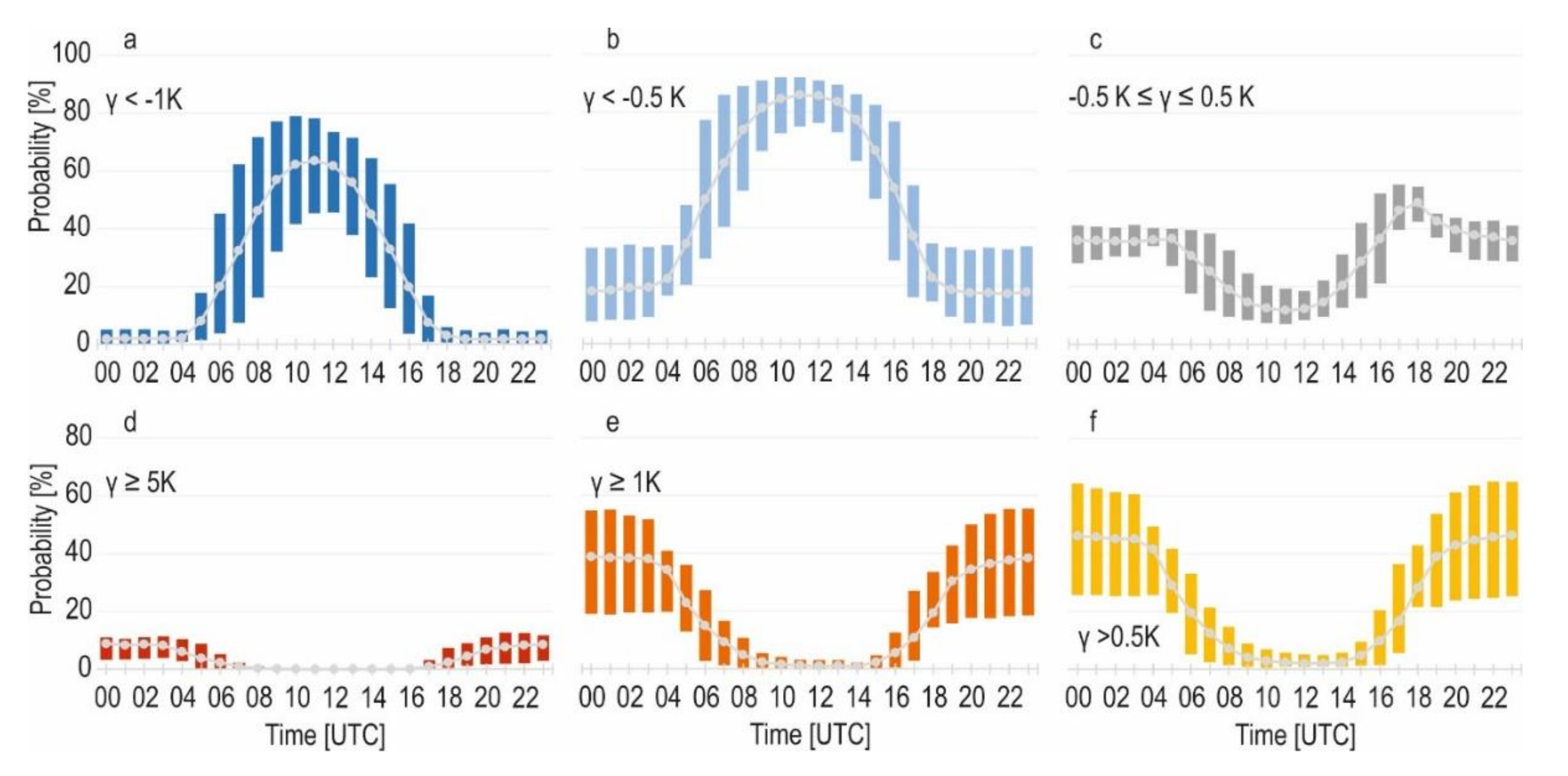
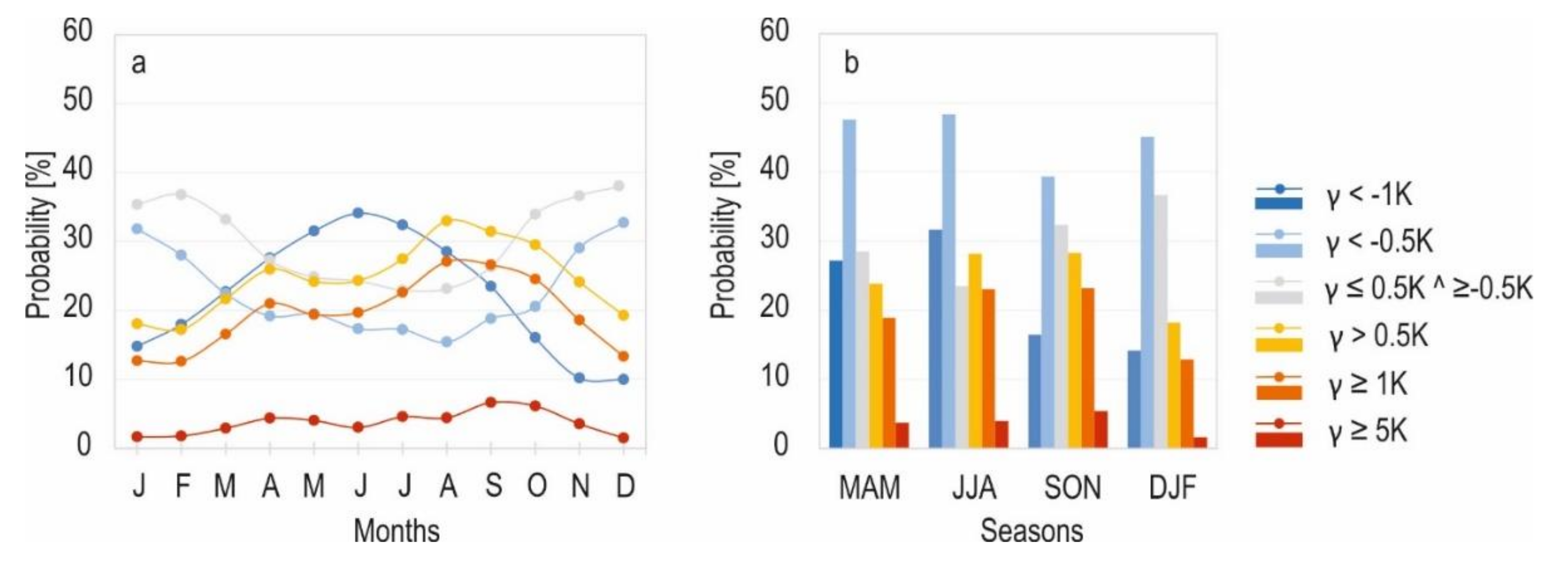
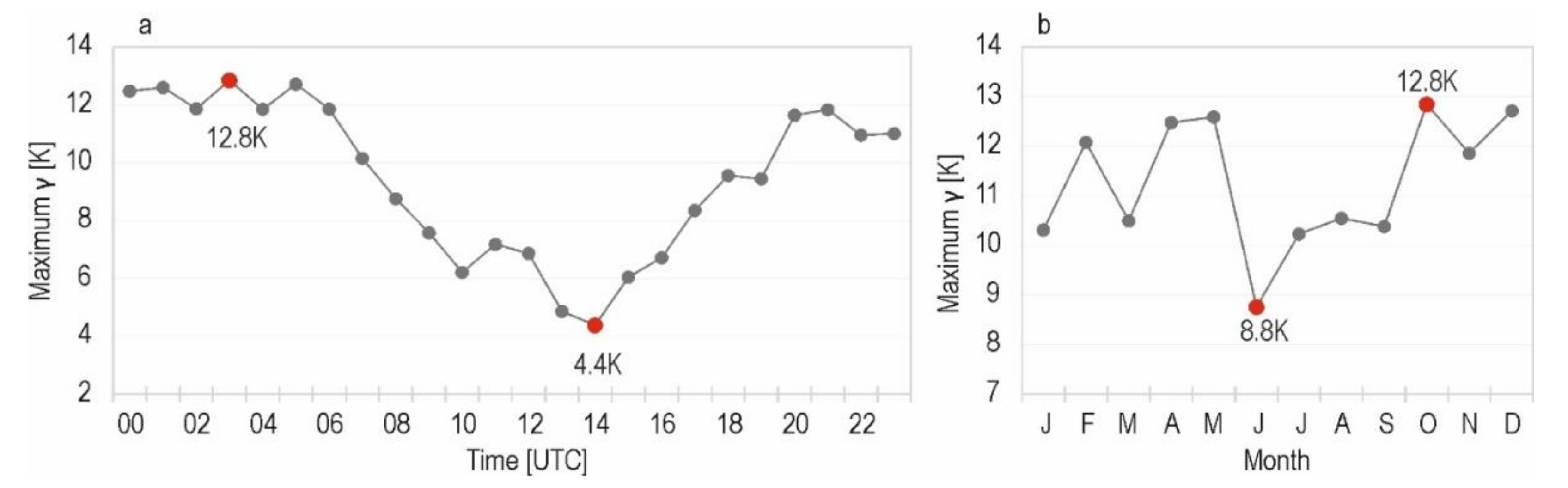
3. Climatology of Air Temperature Gradients—Occurrence, Persistence and Intensity

3.1. Daily Course of Air Temperature Gradients (γ)

The daily courses of the probability of a given air temperature gradient show opposite patterns for unstable and stable air (Figure 3). Grey solid lines with dots in Figure 3 represent daily variability in the probability of a particular γ class calculated for the entire year. The vertical bars show seasonal variability in this probability. The bar bottoms represent the seasonal minimum (various months), while the bar tops represent the maximum seasonal probabilities.

During the daytime, when solar radiation is active, the unstable conditions reached their maximum (>80%) between 09 and 14 UTC (Figure 3a,b). Strong instability reached a maximum probability of 60% during a day and was extremely scarce at night between 19–04 UTC (Figure 3a). The seasonal variability in the probability of unstable conditions was greatest in the morning at 06–09 UTC and in the afternoon at 14–16 UTC (Figure 3a,b). The highest seasonal probability of unstable air between 05–17 UTC, reaching more than 90% midday, occurred in summer, while the lowest probability (07–15 UTC) occurred in winter. In the remaining part of the day, the situation was inverted. The highest seasonal probability between 18–04 UTC usually occurred in winter, while the lowest probability occurred in summer (19–04 UTC) or autumn (05–06 UTC or 16–18 UTC).

SBI usually occurred at night with the maximum probability (more than 40%) taking place between 20 and 03 UTC, and occasionally, during the daytime, it held a probability lower than 10% between 08–16 UTC (Figure 3d–f). Strong SBIs were very rare even at night (10–13% at 20–04 UTC), and they did not occur during the day between 12–15 UTC. Seasonal variability in the daily course of SBI probability was also largest at night.

3.2. Annual Course of Air Temperature Gradients (γ)

Typically, the maximum probability of strong instability (γ < −1 K) appeared during warm months (May: 31.5%, June: 34.1%, July: 32.4%), and the minimum probability appeared in November and December (ca. 10%), which results from the annual variability in solar radiation reaching the Earth’s surface. The annual course of γ < −0.5 K was close to that for isothermal conditions. The occurrence of SBI was most likely to occur in August, followed by September and December (Figure 4a). The secondary maximum was found in May (29.1%). The probability of very strong inversion was highest in autumn (6.6% in October and 6.1% in November) and lowest in winter (1.5–1.8%) (Figure 4b). Such an annual course of the SBI probability is generalized and highlighted by seasonal probabilities of SBI (Figure 4).

The daily and monthly courses of maximum hourly SBI strengths are shown in Figure 5. The strongest SBIs occurred at night between 20 and 06 UTC, when their strength exceeded 11 K/100 m with a maximum of 12.8 K/100 m registered at 03 UTC in October (Figure 5a). The annual pattern is less evident and masked by a wide range of variability between months. The tendency towards low SBI strengths in the warmer part of a year (June-September) can be identified (Figure 5b).

Monthly and seasonal SBI probabilities, depending on their duration and strength, are presented in

Table 3. Monthly and seasonal probability [%] of air temperature inversions of a duration of 1 h, 3 h, 6 h and 12 h calculated based on 1 h data.

Period	γ > 0.5 K				γ ≥ 1 K				γ ≥ 5 K
	1 h	3 h	6 h	12 h	1 h	3 h	6 h	12 h	1 h	3 h	6 h	12 h
Dec	57	45	33	14	45	35	24	8.5	8	5	2.0	0.5
Jan	54	41	31	14	44	32	23	8.8	8	6	2.6	0.3
Feb	61	46	33	10	48	35	25	7.2	10	5	2.8	0.9
DJF	57	44	32	13	46	34	24	8,2	8.8	5.3	2.5	0.6
Mar	69	59	46	15	59	44	34	9.0	17	11	4.9	0.3
Apr	84	74	57	14	77	65	47	7.9	29	17	6.4	0.1
May	86	75	51	5.1	79	66	38	0	29	17	4.0	0
MAM	79	69	51	11	72	58	40	8.5	25	15	5.1	0.2
Jun	88	76	51	3.3	85	71	39	1.3	25	13	2.2	0
Jul	89	82	58	6.4	85	73	47	2.9	33	20	4.1	0
Aug	94	88	73	21	89	80	58	12	31	18	5.2	0
JJA	90	82	61	10	86	75	48	5.4	30	17	3.8	0
Sep	83	75	64	33	76	67	54	26	35	24	11	0.9
Oct	79	69	58	27	70	62	49	20	27	20	11	3.0
Nov	67	56	41	20	57	46	33	15	16	11	6.4	1.6
SON	76	66	54	27	67	58	45	20	26	18	9.5	1.9

γ—air temperature gradient defined as its change per 100 m; 1 h, 2 h etc.—duration of air temperature inversions.

. Generally, short-lasting SBI (1 h, γ > 0.5 K/100 m) was very common. Its probability exceeded 50% throughout the entire year and was higher than 80% between April and September, with apparent domination in summer and a maximum in August. A similar distribution was also characteristic of SBI with 3-h and 6-h durations and for moderate and strong SBI (γ ≥ 1 K) of analogous durations. The maximum probability of the longest SBI (≥12 h) was found in SON on a seasonal scale and in September on a monthly scale, with the exception of the strongest SBI (γ ≥ 5 K), which peaked in October (Table 3).

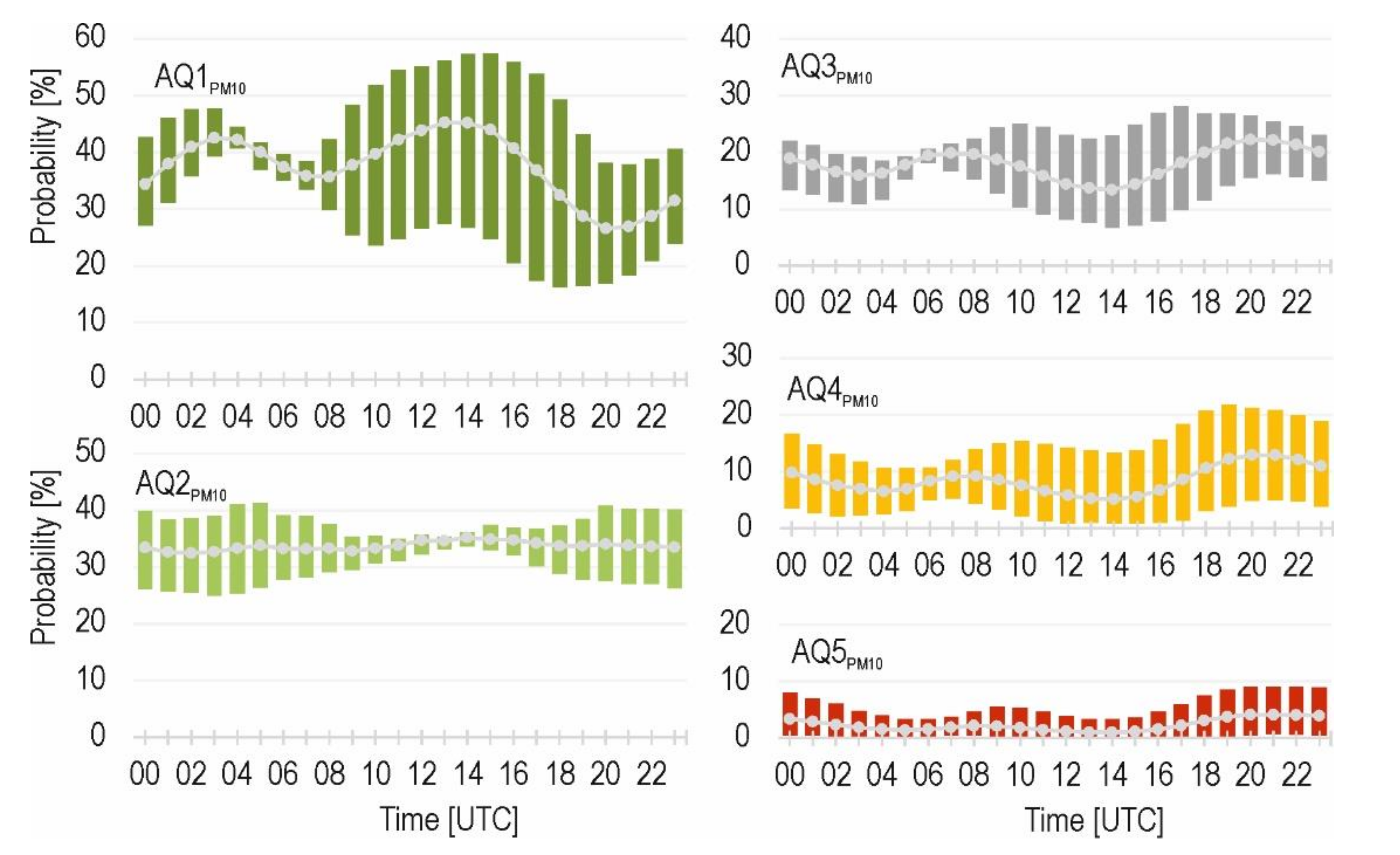
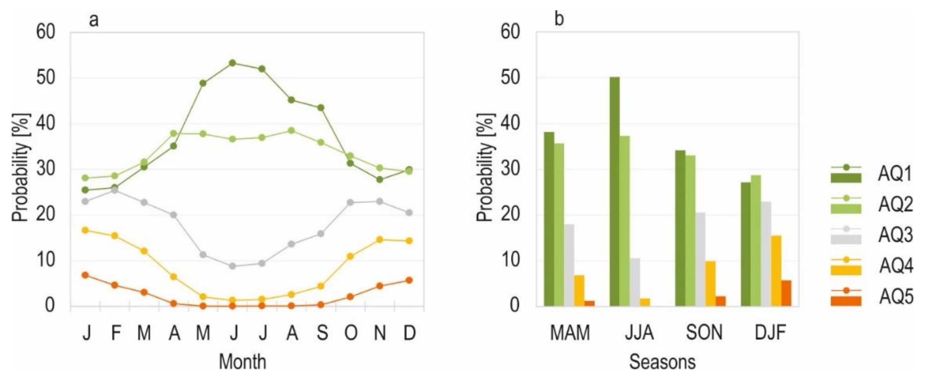
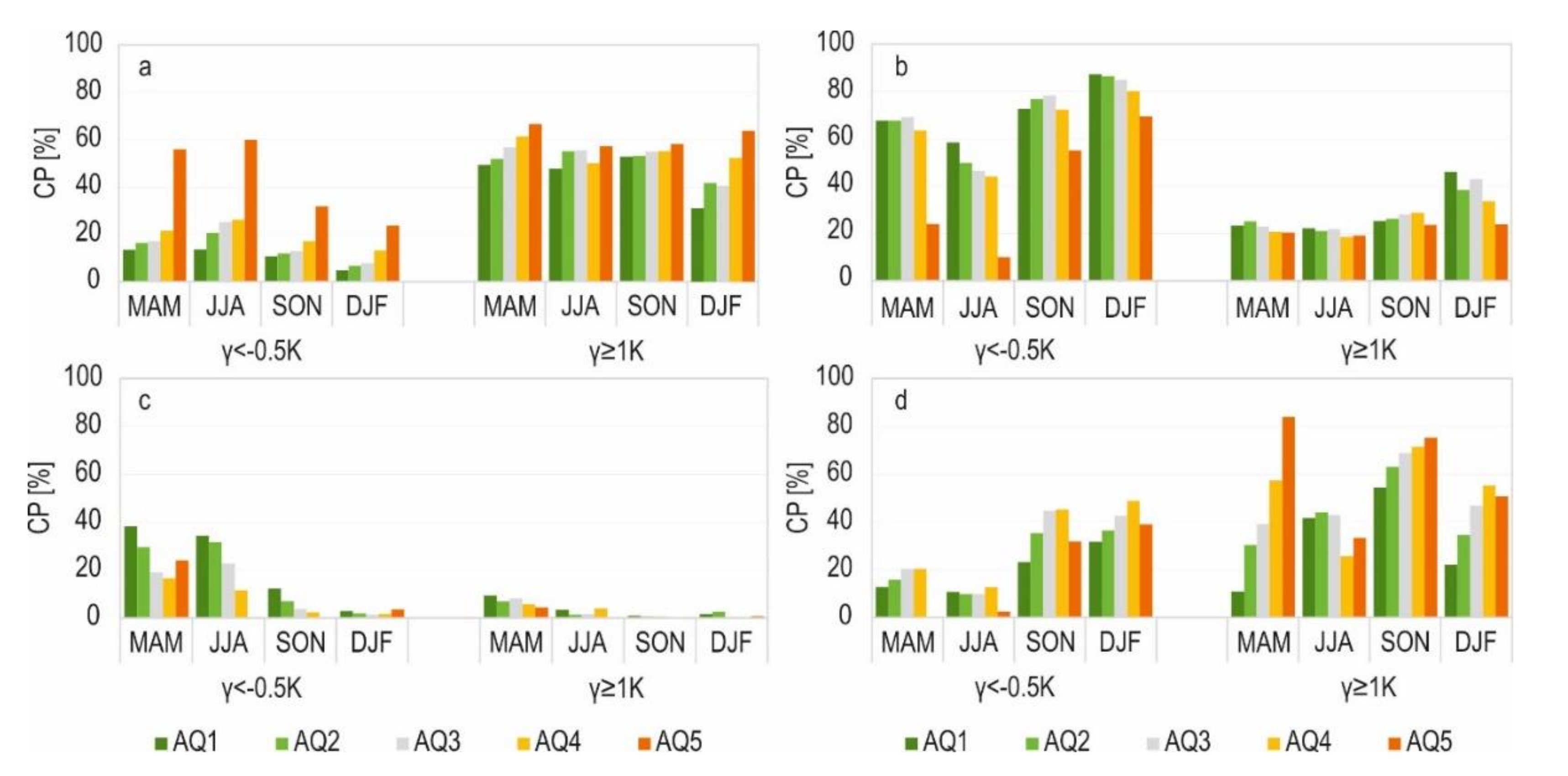
4. Daily, Monthly and Seasonal Variability in Air Quality Classes

Daily courses of the probability of AQ classes are presented in Figure 6. Light grey dots connected with a line represent the annual probabilities, while vertical bars represent seasonal ranges. Although the range of the vertical axis differs depending on AQ, the scales of the axes are the same, so the size of the graph and the degree of variability are comparable to each other. Most of the classes have a clear bimodal daily course, except for AQ2 due to its narrow range of diurnal variability (32–35% probability). AQ1 reached its primary maximum in the early afternoon between 13–15 UTC and was secondary in the early morning between 02–05 UTC (probability >44% annually). Seasonal variability in the AQ1 probability exhibited a wide range between 10 and 18 UTC, with the minimum and maximum values occurring in winter (23% on average) and summer (26% on average), respectively. Little seasonal variability was found between 04 and 06 UTC.

The probability of AQ45 (polluted air) had an inverted daily course compared to the clean air classes of AQ12. The primary maximum of AQ4 occurred in the evening (19–22 UTC), with the highest annual probability at 20–21 UTC (12.9%); the secondary maximum was observed in the morning between 07–08 UTC (9.2%). The winter maximum AQ4 probability was shifted to occur later in the morning (09–10 UTC) and earlier in the afternoon (19–20 UTC) compared to the annual values. A similar daily course was characteristic of a moderate AQ class (AQ3) (Figure 6). The probability of the most polluted air class (AQ5) was highest between 20 and 22 UTC and in the morning between 08 and 09 UTC. The characteristic feature of that class was that a relatively high probability persisted until midnight. In the case of AQ4_, the probability diminished after 20 UTC. The range of seasonal variability in the AQ5 probability class was determined by the winter maximum and summer minimum. Such a daily course of the AQ classes indicates the main sources of PM₁₀ in the GZM, which are mostly domestic premises and transport/traffic (near the ground emission sources). However, very rarely, the AQ5 class also occurred in summer with the exception of the hours between 12 and 14 UTC. Summer episodes of high PM₁₀ concentrations occurred within various hours and on various days depending on the station and were most frequent in Sosnowiec, which suggests their local sources.

Monthly and seasonal variabilities in the AQ probabilities are presented in Figure 7. In the GZM, clean air was most likely to occur in the warm part of a year—between May and July (AQ1 > 50%) or between April and August (AQ2 almost 40%). Polluted air classes were numerous between November and January (AQ4: 14.3–16.7%; AQ5: 4.5–6.8%) (Figure 7a). The seasonal probability of polluted air (AQ45) reached 23.4% in winter and 14.2% in autumn (Figure 7b).

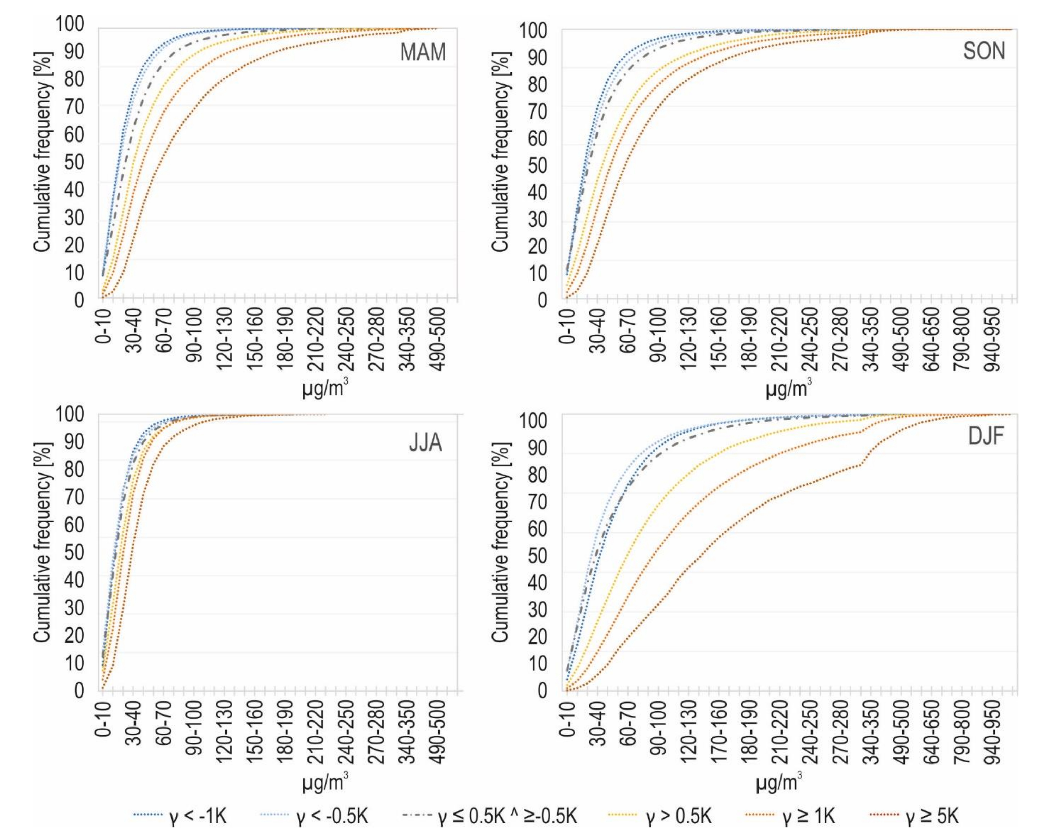
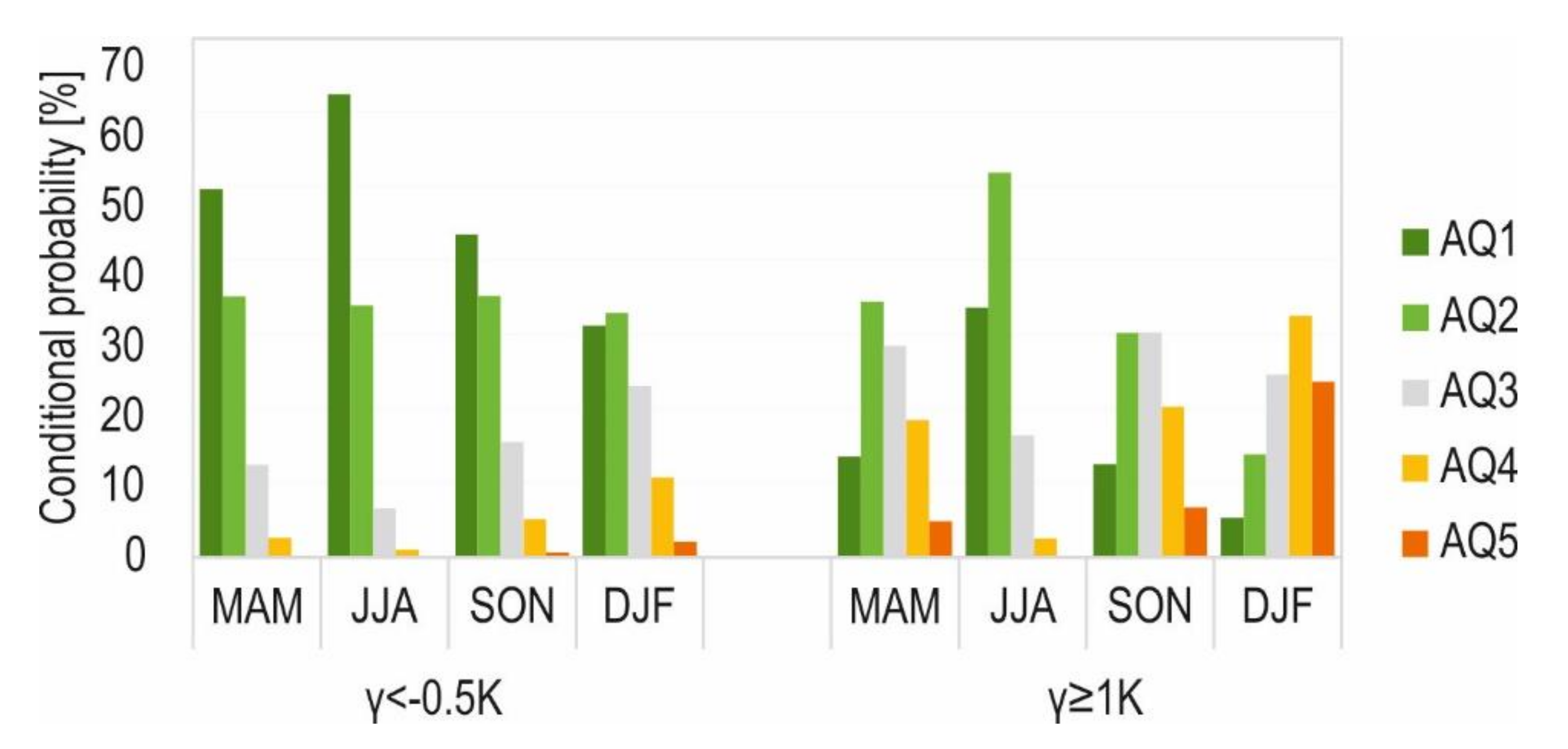
5. Relationships between Air Temperature Gradients and Air Quality Classes

The air quality depends on γ, which is presented in Figure 8, showing the frequency distribution of PM₁₀ concentrations for particular γ classes. The relation between PM₁₀ concentrations and γ varies throughout the year and is the strongest in winter and most noticeable in spring and autumn.

In winter, the PM₁₀ concentrations most frequently reached 20–40 μg/m³ during unstable conditions. In the other seasons, the range with the maximum frequency shifted to 10–20 μg/m³. During weak inversions, the PM₁₀ range of 30–40 μg/m³ was most frequent in winter and spring, while in autumn, a range of 20–30 μg/m³ dominated. Although air was generally clear under unstable conditions, episodes of very high PM₁₀ concentrations (>180 μg/m³) were also noted and constituted approximately 2.3% of the cases occurring in DJF, 0.2% in MAM and 0.6% in SON (values averaged over γ < −1 K and <−0.5 K). The level of pollutants in these conditions depends only on the amount of emissions. During moderate and strong SBI, the most frequent PM₁₀ concentrations were higher, reaching 50–70 μg/m³ in DJF and 30–40 μg/m³ in both transitional seasons. Although these PM₁₀ ranges fall into good and moderate AQ classes, the frequency of hours where PM₁₀ > 90 μg/m³ and 180 μg/m³ was high. In winter, AQ45 occurred during 54% of hours with medium SBI and 73% of hours with strong SBI. AQ5 (PM₁₀ > 180 μg/m³) constituted 22% of hours with medium SBI and 39% of hours with strong SBI. In transitional seasons during moderate SBI, the air was polluted (>90 μg/m³) in 21% (MAM) and 25% (SON) of cases and very polluted (>180 μg/m³) in 4% (MAM) and 6% (SON) of cases. During strong inversions, the situation was worse. The air was polluted in 35% of cases and very polluted in 9% of cases in both seasons.

The highest hourly PM₁₀ concentrations were all noted in winter months, mostly in January at night during moderate or strong inversion, i.e., Sosnowiec—1118 μg/m³ on 12 February 2012 at 21 UTC with γ = 5.1 K; Katowice—672 μg/m³ on January 09, 2017 at 03 UTC with γ = 7.9 K; Zabrze—1236 μg/m³ on January 09, 2017 at 22 UTC with γ = 4.6 K; and Gliwice—824 μg/m³ on 04 January 2002, at 04 UTC with γ = 2.2 K. The maximum winter PM₁₀ concentration occurring during unstable conditions reached 787 μg/m³ on 13 February 2012, at 07 UTC in Sosnowiec, 532 μg/m³ on 10 December 2001, at 01 UTC in Katowice, 767 μg/m³ on 9 January 2017, at 10 UTC in Zabrze and 687 μg/m³ on 04 December 2010, at 23 UTC in Gliwice.

Seasonal variability in the conditional probability (CP) of AQ classes occurring during unstable and stable conditions is presented in Figure 9. The left half of the figure (γ < −0.5 K) represents strong and conditionally unstable conditions, while the right half represents moderate and strong SBI events (γ ≥ 1 K). The CP of clean air (AQ12) dominated the CP of other AQ classes in all seasons during unstable conditions and in summer during SBI (Figure 9). The AQ1 probability varied seasonally from 67.3% in JJA to 34.2% in DFJ during unstable conditions and was similar (36.6%) during SBI in JJA. The occurrence of polluted air (AQ45) was more dependent on air stability and varied seasonally. Both classes of bad and very bad AQ were most likely to occur in winter (AQ4: 36.8%, AQ5: 26.7%) during SBI. In spring and autumn, AQ4 occurrence had a nearly equal probability (20.3 and 21.4%) but decreased by ca. 16% in winter. During SBI, the probability of very bad air quality in transitional seasons (SON: 7.0%, MAM: 5.4%) was 4–5 times lower than that in winter (Figure 9). AQ5 also sporadically registered under strong and conditionally unstable conditions in winter.

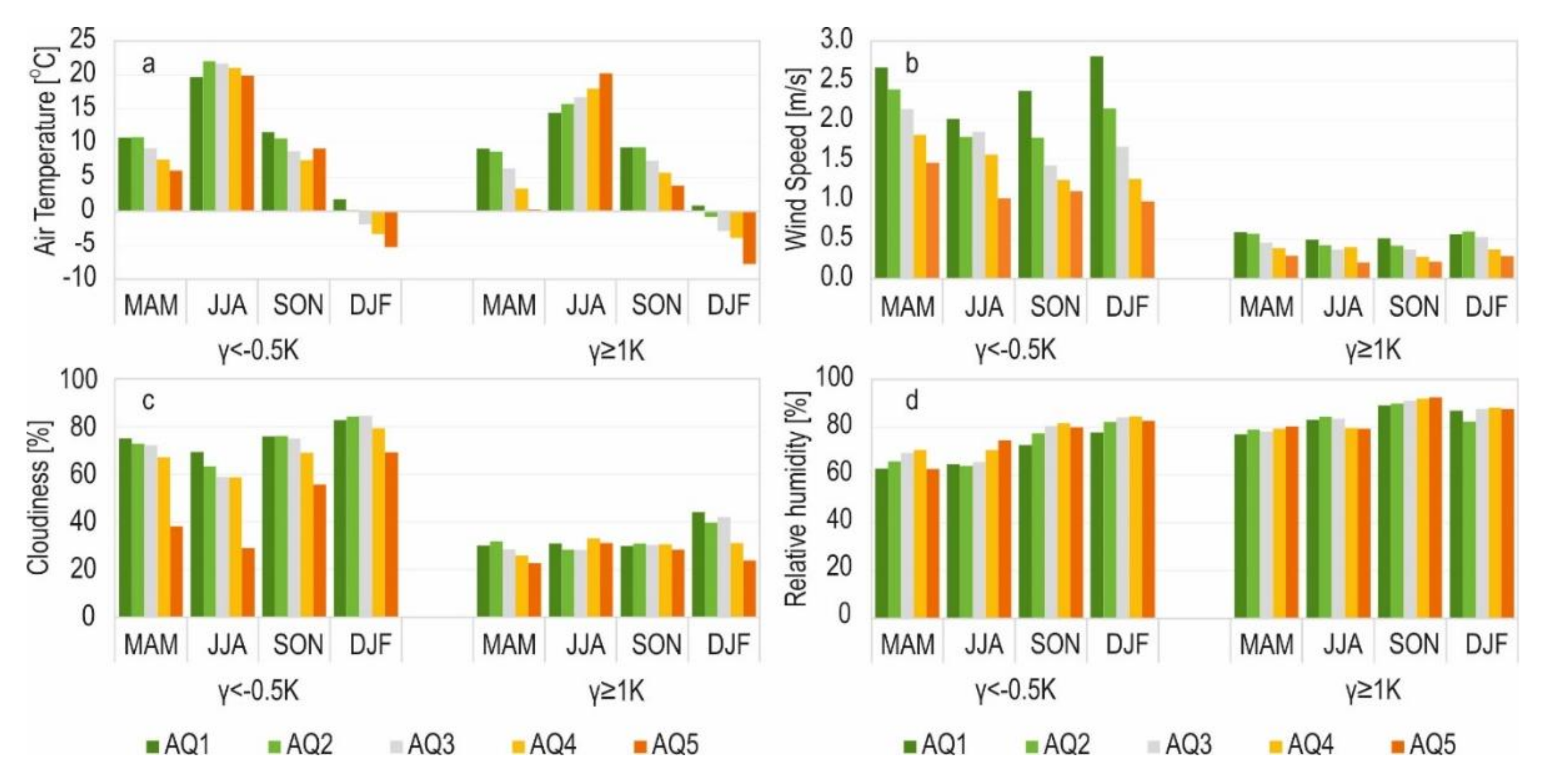
6. Meteorological Conditions for Vertical Temperature Gradients and Air Quality Classes

This section compares the average values of the selected meteorological elements calculated under unstable and stable conditions and for AQ classes. Figure 10, Figure 11 and Figure 12 deliver complex information on these relationships and their seasonal variability. We assumed that the larger the difference in the averages between stable and unstable conditions is, the greater the impact on the formation of SBI. Moreover, we also assumed that the apparent differences in the average values of meteorological elements between the AQ classes during particular seasons (hereinafter called the range of variability) indicate that an element significantly impacts the AQ.

6.1. Air Temperature (AT)

In the case of air temperature, the differences between stable and unstable condition partly results from the daily cycle in their occurrence; however, these differences are not large. The average seasonal AT during SBI, that occurred mostly at night, was reduced by 3.8 °C (JJA) to 1.2 °C (DJF) relative to that during unstable conditions, that occurred mostly during a daytime. In particular seasons, the range of variability in AT depending on AQ was larger during SBI (MAM: 8.9 °C, JJA: 5.8 °C, SON: 5.7 °C, DJF: 8.6 °C) than under unstable conditions (MAM: 4.9 °C, JJA: 2.4 °C, SON: 4.1 °C, DJF: 7.0 °C). In both spring and autumn, the AQ worsened in line with a decrease in air temperature. The AT reached approximately 10 °C during AQ1 and AQ2 and approximately 4 °C (SON) or 0 °C (MAM) during AQ5. In winter, independent of the vertical gradient, the air temperature was close to 0 °C during days with clean air, and it was negative for the other AQ classes, with a minimum for AQ5 reaching −5 °C during unstable conditions and −8 °C during SBI (Figure 10a). In summer, the air temperature was the highest during AQ5; however, the frequency of that AQ5_PM10 class was very low in that season. Moreover, summer AQ5 occurred on various days depending on the station, suggesting local emission sources of PM₁₀.

6.2. Wind Speed (V)

Wind speeds apparently differed during unstable conditions (MAM: 2.1 m/s, JJA and SON: 1.6 m/s, DJF: 1.8 m/s) and SBI (MAM and DJF: 0.5 m/s, JJA and SON: 0.4 m/s), demonstrating that this meteorological element is decisive for SBI development. Low wind speeds during SBI resulted in a small range of variability depending on the AQ, which equaled 0.3 m/s in all seasons. No seasonal variability in this range indicates that the relationships are stable throughout a year. However, the well-known dependency of AQ on reduction in wind speed is still apparent (Figure 10b). During SBI, the average wind speed for AQ5 did not exceed 0.3 m/s, while for AQ1, it varied seasonally between 0.5–0.6 m/s. Wind speed for hours with bad and very bad AQ during unstable conditions was higher than during SBI; however, it was still at least two times lower compared to the very good and good AQ classes and varied seasonally between 1.2 and 1.8 m/s for AQ4 and between 1.0 and 1.5 m/s for AQ5 (Figure 10b).

Table 4. Average values of meteorological elements separately for various γ classes and AQ classes.

ME	γ Class	MAM	JJA	SON	DJF	AQ Class	MAM	JJA	SON	DJF
AT	γ < −0.5K	10.7	21.1	10.4	0.0	AQ12	10.0	19.0	10.0	1.4
	γ ≥ 1.0 K	6.7	16.1	7.7	−3.5	AQ45	4.2	19.8	5.7	−3.3
	Diff.γ	−4.0	−5.0	−2.7	−3.4	Diff.AQ	−5.8	0.8	−4.2	−4.7
V	γ < −0.5 K	2.5	2.0	2.0	2.1	AQ12	2.2	1.6	1.8	2.3
	γ ≥ 1.0 K	0.5	0.5	0.4	0.5	AQ45	0.9	1.0	0.6	0.8
	Diff.γ	−2.0	−1.5	−1.6	−1.6	Diff.AQ	−1.3	−0.5	−1.2	−1.5
N	γ < −0.5 K	72	64	77	85	AQ12	67	59	71	82
	γ ≥ 1.0 K	34	35	36	41	AQ45	45	49	51	59
	Diff.γ	−38	−29	−41	−44	Diff.AQ	−22	−11	−20	−23
RH	γ < −0.5 K	63	60	77	83	AQ12	68	70	81	82
	γ ≥ 1.0 K	78	83	90	86	AQ45	76	75	89	87
	Diff.γ	15	23	13	3	Diff.AQ	9	6	9	5

AT [°C]—air temperature, V [m/s]—wind speed, N [%]—cloudiness, RH [%] –relative humidity, Diff.γ—difference between γ < −0.5 K and γ ≥ 1.0 K, Diff.AQ—difference between AQ12 and AQ45, values for summer are in grey due to low frequency of bad and very bad air quality in that season.

includes meteorological elements averaged separately for the AQ and γ classes. As stated in the previous section, we assumed that the apparent differences in the weather elements between stable and unstable conditions or between clean and dirty conditions can be used to indicate the relationships between these variables. Only in the case of air temperature were the differences between AQ classes larger than the differences between γ classes. However, it should be repeated that this difference also results from the fact that most SBI occur during the night, while unstable conditions mainly occur during the daytime, which is usually warmer than the night-time. In the case of other elements, the differences suggested their more substantial impact on SBI than AQ (Table 4).

6.3. Cloudiness (N)

Differences in cloudiness between unstable conditions (55–80% on average) and SBI (28–36% on average) are also apparent in Figure 10, which indicates its more substantial role in SBI development than for AQ. During SBI, the range of cloudiness variability with respect to AQ was largest in DJF (20.3%), noticeable in MAM (9.2%) and minor in SON (2.6%) and JJA (4.8%). This means that in winter and to a lower degree in MAM, cloudiness alters AQ. For example, in DJF, the cloudiness was approximately 24% for AQ5_PM10 and one time higher (44%) for AQ1. During unstable conditions, the range of cloudiness variability depending on AQ during a particular season was higher, mostly due to the much lower cloudiness for AQ5 compared to other classes of AQ (Figure 10c). Thus, a reduction in cloudiness also favors the occurrence of very bad AQ5 during unstable conditions (Figure 10). However, it must be noted that the frequency of AQ5 during unstable air was low in most seasons, particularly in JJA.

6.4. Relative Humidity (RH)

The average humidity revealed minor differences depending on both the air temperature gradient and AQ. In all seasons, it was slightly higher during SBI than unstable conditions by about 12–14%, except for winter, when the difference was so slight that it was negligible (4%). The range of variability depending on AQ was also small, which together implies the nature of the weak relationships between RH, SBI and AQ (Figure 10).

Aside from meteorological elements that are known to influence air quality and SBI, we also determined the frequency of wet (RH ≥ 90%) and dry (RH ≤ 50%) hours and clear (N ≤ 20%) and cloudy (N ≥ 80%) hours during the occurrence of particular AQ and γ classes. The results of these analyses are presented in Figure 11d.

6.5. Wet and Dry Hours

Wet hours were more common during SBI; they occurred during 10 (JJA) to 22% (SON) of hours under unstable conditions as averaged over all AQ, while they constituted 37.5 (JJA) to 66.7% (SON) of cases during SBI. Excluding summer, during SBI, the frequency of wet hours increased in line with worsening AQ. The range of variability in the frequency of wet hours depending on AQ during SBI reached 21% in SON, 33% in DJF and 73% in MAM. For example, in MAM during SBI, wet conditions occurred during more than 80% of hours with AQ5, and in other seasons, wet conditions constituted 75% (SON) and 50.7% (DJF) of hours with AQ5. It can be concluded that wet conditions favor the occurrence of both SBI and polluted air in most seasons except for summer. This conclusion is also supported by the frequency of dry days (Figure 11), which constituted an irrelevant percentage of hours with SBI. However, dry days are generally infrequent in the temperate climate type of Poland and the GZM. The maximum probability of dry hours (9% for AQ1) during stable conditions was reached in MAM. During unstable conditions, dry hours were most frequent in MAM and JJA and constituted 30–40% of hours with clean air (AQ1 and AQ2).

6.6. Clear and Cloudy Hours

It has already been shown that cloudiness is a crucial element impacting the occurrence of SBI and, to a lesser extent, AQ. We decided to further study the relationships between these elements and considered the probability of clear and cloudy hours conditioned by AQ and γ. Clear hours occurred much more frequently during SBI and constituted, on average, 55–60% of SBI cases, except for DJF (46%). Cloudy hours dominated during unstable conditions (on average, more than 60% to 80% of cases), excluding summer (Figure 11). During SBI, the percentage of clear hours varied depending on AQ in DJF, thereby impacting air quality. An increased probability of clear hours was also found during unstable conditions, particularly for AQ5 in MAM and JJA (a small number of cases), i.e., approximately 60% for AQ5 vs. 10–20% for other AQ classes (Figure 11). It can be concluded that a low cloudiness favors the occurrence of SBI and AQ5.

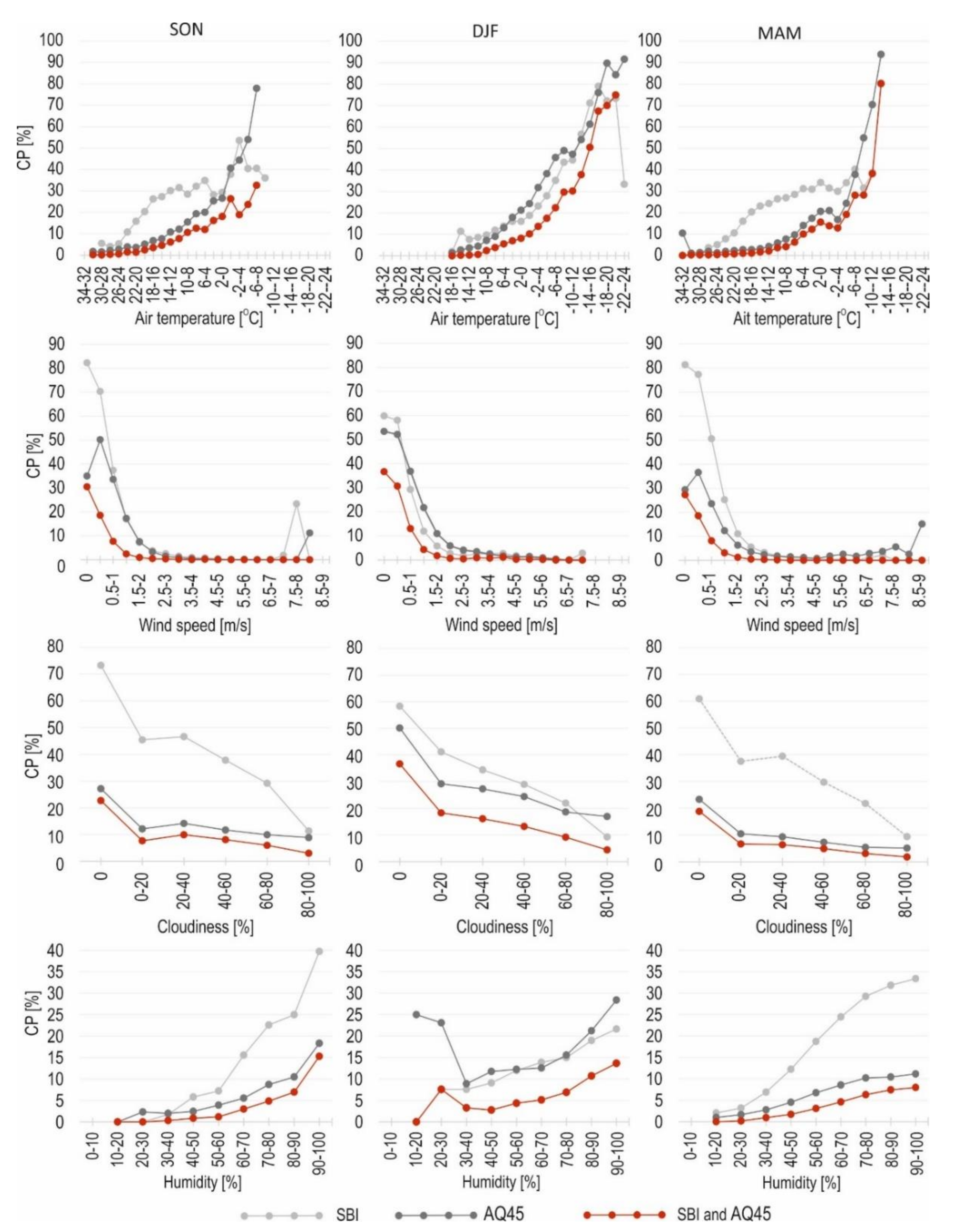
7. Probability of Air Temperature Inversions and Bad Air Quality Conditioned by Ranges of Weather Elements

In this section, the conditional probability (CP) of AQ45 and SBI for particular ranges of meteorological elements is discussed. Such analysis enabled us to identify the specific values of weather elements with the highest probability of SBI and AQ45 and distinguish the thresholds for a clear increase/decrease in the probabilities (SBI and AQ45). Figure 12 shows the CP of SBI (light grey line), AQ45 (dark grey line) and simultaneous SBI and AQ45 (red line, hereafter AQ45 and SBI) for particular ranges of air temperature, wind speed, cloudiness and humidity. The highest probability is the essential role of an element in the development of SBI or bad AQ. Similar to the previous sections, we excluded summer due to the low frequency of AQ45.

The most important factor driving the occurrence of AQ45, AT, had strongest influence in MAM and DJF; the highest CP of AQ45 reached 94% and 92%, respectively, while the maximum probability of joint AQ45 and SBI occurrence reached 80% (MAM) and 75% (DJF). The CP of AQ45 and SBI was accelerating by 2% when AT dropped below 8 °C in MAM and SON and 0 °C in DJF. CP enhancement was faster below −2 °C in SON, −6 °C in DJF and −4 °C in MAM. The role of AT on SBI and AQ45 varied depending on the range of AT.

In the case of other meteorological elements, the maximum probability of AQ45 in the period 1993–2020 during SBI was much lower; however, the apparent acceleration of CP indicates wind speed as the second most important driver of AQ45 during SBI. In each season, the maximum probability of AQ45 and SBI, reaching approximately 40%, was a characteristic of calm (0 m/s) conditions, and it rapidly dropped in line with increasing wind speeds to less than 3% at 1.5 m/s. Wind speed impacts the SBI occurrence to the greatest extent, which is indicated by a very high CP within the low wind speed range, particularly in SON and MAM (more than 80%, Figure 12). A rapid increase in the CP of AQ45 and SBI was found below 2–2.5 m/s. The relationships between SBI, AQ and wind speed did not change seasonally.

The CP of the joined SBI and AQ45 event was also enhanced by a clear sky. However, the maximum CP found during the cloudless hours (N = 0%), reaching 19% (MAM) to 37% (DJF), was lower than the maximum AT and wind speed. The development of cloudiness (N > 20%) decreased the CP to less than 10% in SON and MAM and 18% in DJF. For N > 20%, the CP reduction in the subsequent N ranges was much smaller (Figure 12). Cloudiness had the strongest impact on SBI, in SON and MAM. The CP of SBI reached a maximum of 70–60% during cloudless hours (N = 0%) and was at least 40% for the cloudiness range of 20–40%. The probabilities of AQ45 and SBI were almost equal during cloudy hours (N = 100%) (Figure 12).

The impact of relative humidity on SBI and AQ45 was the weakest of all meteorological elements. The maximum probability of AQ45 and SBI varied between 8% (MAM) and 15% (SON) during hours with RH in the range of 80–100% and was lower than 10% for most of the RH range. The high CP of AQ45 for RH < 30% results from the low number of cases and should be disregarded. Moreover, the RH more strongly impacted the development of SBI than the occurrence of bad AQ. This is demonstrated by a steeper increase in SBI probabilities between RH 20% and 80%.

8. Discussion

The GZM was shown to be a seriously polluted area. The average annual concentration of PM₁₀ in its central part (Sosnowiec: 44.7 μg/m³, Katowice: 43.5 μg/m³, Zabrze: 47.6 μg/m³, and Gliwice: 50.1 μg/m³) was higher by at least 50% compared to other European cities such as Bern: 35.9 μg/m³, Basel: 22.9 μg/m³, Zurich: 24.0 μg/m³, Lugano: 33.0 μg/m³ [86], Liverpool: 25.0 μg/m³ [87], and Helsinki: 18.7 μg/m³ [88], and was lower by only 6 μg/m³ compared to Tel Avive (50 μg/m³), which is impacted by the transport of mineral dust from the surrounding deserts [89]. Although our study concerns PM₁₀ concentrations, it is also representative of PM₂.₅ since many studies have indicated a strong correlation between these variables [81,86]. In the GZM, PM₂.₅ has only been measured in Katowice since 2009, and the series includes many gaps.

Analyzed as a background, the climatology of γ and AQ showed that the daily course of various γ follows the daily cycle of solar radiation that peaks at midday and results in the extreme probability of unstable conditions [6] in summer (maximum) and winter (minimum). The wide seasonal range of the probability of unstable conditions during a day results from varying a solar angle throughout the year. The daily course of SBI in the GZM area is also typical, with most SBIs occurring at night when radiative cooling prevails [45,61,90,91]. The probability of summer nocturnal SBI in the GZM area is comparable to its probability in other parts of southern Poland, as described by Palarz et al. [45], who used reanalysis data. However, the probability of winter nocturnal SBI was lower in the GZM area (approximately 25%) than in southern Poland (40–50% by Palarz et al. [45]), which may confirm the findings of a previous study by Bokwa [42], which indicated the lower frequency of winter SBI in an urban environment than in its surroundings. This can be attributed to the large heat capacity and increased thermal turbulence of cities [92]. A comparable probability of winter nocturnal SBI was noted in Łeba, which is located at the sea coast where the air is more dynamic [44]. In the GZM, the strongest and longest SBI occurred in autumn when wind speeds and cloudiness factors were lower than those in winter [93]. The frequency of all day-round SBI is low, unlike that observed at higher latitudes [8,23,24,27,32,94,95] and in concave terrains [9,26,70,96,97], due to shorter nights and milder weather conditions and more exposure to general weather conditions in upland conditions than in valleys and basins. Daytime SBI mainly occurs in summer, when favorable weather conditions for SBI development are more frequent than in winter. These conditions include lower wind speeds and cloudiness. Although rare, all-day SBIs at temperate latitudes are usually related to the general synoptic situation and are frequently of the advective type [98]. The role of high-pressure systems, wedges or anticyclonic ridges on SBI development regardless of whether they occur during the daytime has been confirmed in many studies [33,61,91,98,99,100,101,102,103,104], including those completed in the GZM area [98,105]. Large-scale circulation can also lead to a strengthening of near-surface inversion [106].

The annual course of unstable conditions was also typical, with a maximum probability in summer and June when the longest days, maximum global radiation and highest daily effective sunshine occurred in Poland [93]. Outside the city, where seasonal changes in types of ground cover play an influential role (vegetation), the maximum probability of unstable conditions can be shifted to months with initial vegetation due to the rapid warming of the surface, with a low amount of heat absorbed during transpiration, which was found in Moscow and its suburbs [54].

Our study indicated apparent bimodal SBI distributions with a primary maximum in August and secondary maximum in April and minimums in December and June. Such an annual course also slightly differs from that found in Łeba in northern Poland, where a comparably high frequency of SBI persists from April to August but minimum also occurred in winter [44]. The lowered probability of SBI in the GZM area can result from the warmer urban surface in the warmest months of a year. Apart from these differences, generally, the summer maximum and winter minimum of SBI probability are driven by the annual cycle of wind speed, the number of clear and cloudy conditions and the net longwave radiation in Poland [93]. The highest probability of the longest and strongest SBI in SON (not in DJF) results from the lower wind speed and cloudiness in that season in the GZM area compared to that in DJF. In Teheran, the strongest SBI also occurs in SON [79].

The daily and annual courses of the AQ classes are linked to the activity of urban inhabitants. The highest probability of moderate and bad AQ coincided with rush hour (07–08 UTC and 20 UTC), as is the case in many other urban areas e.g., [107,108,109,110]. The probability of AQ5 remained relatively high throughout the entire night because the very bad air quality usually occurred during very low air temperatures and was related to more intense emissions in the near the ground level of atmosphere. Moreover, frosty conditions are usually associated with clear nights promoted by anticyclonic conditions that enhance SBI intensity and duration. The nocturnal maximums of the AQ4 and AQ5 probabilities are compatible with increased night-time SBI occurrence. The similarities in the daily course of these phenomena are not surprising and have already been reported by many studies [57,58,59,76,111,112,113,114,115,116]. In contrast, the annual courses of SBI and the bad and very bad AQ class were opposite. However, although rare, winter inversions are of utmost concern due to enormously intense emissions in the lowest part of air on winter freezing nights in this region. In the GZM, the maximum hourly PM₁₀ concentrations occurred in winter during SBI and were higher than the threshold for the very bad AQ class (>180 μg/m³) by 350% to more than 600% depending on the city. In the GZM, the permissible number of polluted days (35 days a year) is exceeded by more than 200% in most cities of Metropolis, with a maximum of more than 400% (140 days a year) in Wodzisław Śląski about 55 km on SW from Sosnowiec (not analyzed in this study). Most of the hours with AQ5 occurred in the winter months.

The influence of weather conditions on γ and AQ depended on weather elements and seasons. The relationships between SBI, AQ and weather conditions in the GZM located in the upland area may be more complicated than those under concave terrain. This can be concluded based on Whiteman et al. [9], who found that the mechanism of SBI development and dissipation in basins are more complicated than those in valleys, where the atmosphere is better protected by the surrounding topography from synoptic-scale flow intrusions. In the GZM, the wind most directly and immediately affected the SBI dissipation, particularly in SON and MAM, when the probability of SBI reached more than 80% during calm condition and ca. 70% under wind speeds up to 0.5 m/s. In most studies based on daily data, winds below 3 m/s [65], or below 4 m/s [64] were found to be most favorable to SBI build-up. Our study determined that these speeds act as thresholds below which a noticeable increase in SBI probability was found. The hourly average wind speed during SBI (V ≤ 0.5 m/s) is lower than the daily averages because the latter also includes speeds during the daytime when SBI is rare. The impact of wind speed on AQ was noticeable under both stable and unstable conditions. Low wind speeds also significantly affect AQ in other locations e.g., [66,67,68,69,70,71]. However, in the GZM, the regional wind speed can be more important than in other cities located in concave terrains that are isolated by topography, which causes reduced wind speeds [15]. The increased wind speed may also have an adverse effect on air quality in the case of the long-range transport of pollutants [76] or recirculation from surrounding emitters [117].

Probability analysis indicated that air temperature triggered air quality reductions, particularly in winter, because it determines the intensity of emissions in the lowest part of atmosphere (heating of houses). The effect of air temperature is minor in summer but only during unstable conditions when the variation in air temperature between the AQ classes was small. However, the episodes of bad AQ in summer were sporadic with a slightly enhanced frequency in Sosnowiec, which implies the local nature of the sources of these episodes. Our previous study of biomass burning organic tracers based on year-round samplings in Sosnowiec indicated an enormously high concentration of levoglucosan during summer [118]. This may indicate the local burning of biomass on allotment gardens and home fireplaces, which, as a consequence, elevate the PM₁₀ concentrations in summer.

We also found that most bad AQ cases in summer during unstable conditions occurred in the morning between 06–07 UTC (much more common), while bad AQ occurrence under stable conditions was mostly noted in the evening between 19 and 21 UTC. Some of these episodes might have had external sources and could have been related to atmospheric circulation. Previous research showed that in Sosnowiec during JJA, the highest/enhanced PM₁₀ concentration was found during southerly and south-westerly air advection under the influence of anticyclones [112,119]. Such air advection usually causes an increase in air temperature and possible inversion of certain advection types [98].

The highest air temperature observed in summer and the lowest observed in winter are frequently linked to anticyclonic conditions, with a frequently low cloudiness favoring radiative cooling. Consequently, we found cloudiness to be an important factor for SBI development, but its role in AQ was much lower and limited to clear hours (N ≤ 20%), which also enhanced the concentration of PM₁₀ during unstable conditions. All cases of enhanced PM₁₀ concentrations during unstable conditions and clear hours (N ≤ 20%) were also accompanied by low wind speeds and negative air temperatures. We speculate that unstable conditions occurring during clear hours, low wind speeds and low air temperatures could have been limited to the urban environment due to the presence of heat islands that prevented SBI development in the city but not outside the city. This, however, needs further research.

The relative humidity varied little depending on both γ and AQ. Stronger relations were found when only dry (RH < 20%) and humid (RH > 90%) hours were considered. We suppose that the relationship between γ, AQ and RH could be, to some degree, an indirect effect of the relationships between air temperature and SBI due to the well-known inverse association of RH and AT. Moreover, the complicated relationships between γ, AQ and humidity can rise from the fact that the RH in Poland is relatively high and does not vary substantially within a year [93]. The impact of RH on air quality and temperature inversion may be more apparent in more arid climates or areas with more a variable RH throughout the year. We noticed that in transitional seasons (MAM and SON), when the humidity was generally lower than in winter, its relationship with SBI was stronger, as shown by a noticeable increase in SBI probability in line with an increasing RH. However, in some studies, the correlation between RH and air pollution was significant [39,120].

9. Conclusions

In summary, it is complicated to quantify the role of particular meteorological elements on γ and AQ due to interactions between the meteorological elements. However, it is clear that air temperature determines the intensity of PM₁₀ emissions, thereby affecting its concentration in the air, which is seriously enhanced by SBI, particularly in winter. SBI is directly related to wind speed and the degree of cloudiness, which determines the intensity of radiative cooling and the development of SBI and a further decrease in temperature, which translates to an increased relative humidity. In SON and MAM, cloudiness drives SBI more than air temperature. In winter, the impact of air temperature on SBI rises, and the maximum SBI probability conditioned by AT is higher than that conditioned by cloudiness. The relative humidity exhibits a weaker impact on AQ and SBI than all other elements. The relation between RH, AQ and SBI could, to some degree, result from its strong correlation with air temperature.

The maximum probability of strong SBI (γ > 5 K) in the early morning (03-06 UTC) and early evening (17-19 UTC) was found in autumn.

In the annual course, the SBI probability reached its maximum between April and August. The bimodal shape of the annual course of SBI caused by a reduced SBI occurrence in May, June and July may result from solar heating of urban surfaces that diminish the frequency of surface based inversions.

Although the most intense and longest SBI occurred in SON, winter SBI events are of profound importance due to their strong impact on air quality in the GZM.

Air quality heavily depended on the air temperature gradient, particularly in winter, when the PM₁₀ concentrations were the highest. Bad and very bad air quality (>90 μg/m³) constituted 54% and 73% of cases during moderate and strong SBI, respectively. During SBI in winter, the probability of AQ5 was 4–5 times higher than that in transitional seasons and 12 times higher than that during unstable conditions.

Air temperature strongly impacts AQ, particularly in winter during SBI in clear and calm nights. Wind speed is crucial for SBI development and significant for AQ. A low cloudiness also favours the occurrence of SBI, alters air quality in winter and spring during stable conditions and favours the occurrence of AQ5. Wet conditions (RH > 90%) favour the occurrence of both SBI and polluted air except in summer. Smog episodes (AQ45 during fog) mainly occurred in autumn and winter, and they constituted a maximum of 20% of cases with AQ5 in MAM during SBI.

The probability of oppressive episodes of high PM₁₀ concentrations enhanced by SBI rapidly increases in the GZM area when the air temperature drops below −2 °C in SON, −6 °C in DFJ and −4 °C in MAM, the wind speed decreases below 1.5 m/s in SON and DJA and 2.5 m/s in MAM, and the sky is clear (N = 0%) regardless of the season. A change in RH did not cause a notable change (more than 5%) in the conditional probability of AQ45 during SBI.

References

1. Allen, M.A.; Holmes, B.A. Seasonal and Diurnal Patterns of Temperature Inversion Formation and Breakup in a Topographically Complex Urban Environment. In Proceedings of the National Conference on Undergraduate Research (NCUR) 2015, Cheney, WA, USA, 16–18 April 2015; pp. 430–438. [Google Scholar]
2. Holzworth, C.G. Estimates of mean maximum mixing depths in the contiguous United States. Mon. Weather Rev. 1964, 92, 235–242. [Google Scholar] [CrossRef] [Green Version]
3. Elsom, D.; Chandler, T. Meteorological controls upon ground level concentrations of smoke and sulphur dioxide in two urban areas of the United Kingdom. Atmos. Environ. (1967) 1978, 12, 1543–1554. [Google Scholar] [CrossRef]
4. Pissimanis, D.; Karras, G.; Notaridou, V. On the meteorological conditions during some strong smoke episodes in Athens. Atmos. Environ. Part B Urban Atmos. 1991, 25, 193–202. [Google Scholar] [CrossRef]
5. Wang, X.Y.; Wang, K.C. Estimation of atmospheric mixing layer height from radiosonde data. Atmos. Meas. Tech. 2014, 7, 1701–1709. [Google Scholar] [CrossRef] [Green Version]
6. Oke, T.R. Boundary Layer Climates; Routledge: London, UK; New York, NY, USA, 1987; p. 435. [Google Scholar]
7. Sager, L. Estimating the effect of air pollution on road safety using atmospheric temperature inversions. J. Environ. Econ. Manag. 2019, 98, 102250. [Google Scholar] [CrossRef]
8. Serreze, M.C.; Schnell, R.; Kahl, J.D. Low-Level Temperature Inversions of the Eurasian Arctic and Comparisons with Soviet Drifting Station Data. J. Clim. 1992, 5, 615–629. [Google Scholar] [CrossRef]
9. Whiteman, C.D.; Bian, X.; Zhong, S. Wintertime Evolution of the Temperature Inversion in the Colorado Plateau Basin. J. Appl. Meteorol. 1999, 38, 1103–1117. [Google Scholar] [CrossRef]
10. Malingowski, J.; Atkinson, D.; Fochesatto, J.; Cherry, J.; Stevens, E. An observational study of radiation temperature inversions in Fairbanks, Alaska. Polar Sci. 2014, 8, 24–39. [Google Scholar] [CrossRef] [Green Version]
11. Juda, J.; Chróściel, S. Ochrona Powietrza Atmosferycznego [Atmospheric Air Protection]; Wyd. Nauk. Techn.: Warszawa, Poland, 1974; p. 439. (In Polish) [Google Scholar]
12. Bil, G. Prawdopodobieństwo Występowania Inwersji Temperatury Powietrza W Sosnowcu. In Górnośląsko-Ostrawski Region Przemysłowy: Wybrane Problemy Ochrony i Kształtowania Środowiska; Materiały Sympozjum Polsko-Czeskiego; Pełka-Gościniak, J., Rzętała, M., Eds.; University of Silesia: Sosnowiec, Poland, 1999; pp. 33–36. (In Polish) [Google Scholar]
13. Bil, G. Meteorologiczne wskaźniki zapylenia atmosfery (Katowice 1981–1996). Pol. Tow. Mineral. Pr. Spec. 1999, 15, 21–26. (In Polish) [Google Scholar]
14. Corsmeier, U.; Kossmann, M.; Kalthoff, N.; Sturman, A. Temporal evolution of winter smog within a nocturnal boundary layer at Christchurch, New Zealand. Theor. Appl. Clim. 2005, 91, 129–148. [Google Scholar] [CrossRef]
15. Oleniacz, R.; Rzeszutek, M. Assessment of the Impact of Spatial Data on the Results of Air Pollution Dispersion Modeling. Geoinform. Pol. 2014, 13, 57–68. [Google Scholar] [CrossRef]
16. Trinh, T.T.; Le, T.T.; Nguyen, T.D.H.; Tu, B.M. Temperature inversion and air pollution relationship, and its effects on human health in Hanoi City, Vietnam. Environ. Geochem. Health 2018, 41, 929–937. [Google Scholar] [CrossRef]
17. Cohen, L.; Helmig, D.; Neff, W.; Grachev, A.; Fairall, C. Boundary-layer dynamics and its influence on atmospheric chemistry at Summit, Greenland. Atmos. Environ. 2007, 41, 5044–5060. [Google Scholar] [CrossRef]
18. Huff, D.M.; Joyce, P.L.; Fochesatto, G.J.; Simpson, W.R. Deposition of dinitrogen pentaoxide, N2O5, to the snowpack at high latitudes. Atmos. Chem. Phys. Discuss. 2011, 11, 4929–4938. [Google Scholar] [CrossRef] [Green Version]
19. Chen, N.; Guan, D.; Jin, C.; Wang, A.; Wu, J.; Yuan, F. Influences of snow event on energy balance over tem-perate meadow in dormant season based on eddy covariance measurements. J. Hydrol. 2011, 399, 100–107. [Google Scholar] [CrossRef]
20. Bowling, S.A.; Ohtake, T.; Benson, C.S. Winter Pressure Systems and Ice Fog in Fairbanks, Alaska. J. Appl. Meteorol. 1968, 7, 961–968. [Google Scholar] [CrossRef] [Green Version]
21. Bradley, R.S.; Keimig, F.T.; Díaz, H.F. Climatology of surface-based inversions in the North American Arctic. J. Geophys. Res. Space Phys. 1992, 97, 15699–15712. [Google Scholar] [CrossRef] [Green Version]
22. Frederiks, T.M.; Christopher, J.T.; Sutherland, M.W.; Borrell, A.K. Post-head-emergence frost in wheat and barley: Defining the problem, assessing the damage, and identifying resistance. J. Exp. Bot. 2015, 66, 3487–3498. [Google Scholar] [CrossRef] [Green Version]
23. Kahl, J.D. Characteristics of the low-level temperature inversion along the Alaskan Arctic coast. Int. J. Clim. 1990, 10, 537–548. [Google Scholar] [CrossRef]
24. Kahl, J.D.; Serreze, M.C.; Schnell, R. Tropospheric low-level temperature inversions in the Canadian Arctic. Atmos. Ocean. 1992, 30, 511–529. [Google Scholar] [CrossRef]
25. Hartmann, B.; Wendler, G. Climatology of the winter surface temperature inversion in Fairbanks, Alaska. In Proceedings of the 85th Annual Meeting of the American Meteorological Society, San Diego, CA, USA, 9–13 January 2005; pp. 1–7. [Google Scholar]
26. Whiteman, C.D.; Zhong, S. Downslope Flows on a Low-Angle Slope and Their Interactions with Valley Inversions. Part I: Observations. J. Appl. Meteorol. Clim. 2008, 47, 2023–2038. [Google Scholar] [CrossRef] [Green Version]
27. Bourne, S.; Bhatt, U.; Zhang, J.; Thoman, R. Surface-based temperature inversions in Alaska from a climate perspective. Atmos. Res. 2010, 95, 353–366. [Google Scholar] [CrossRef]
28. Bintanja, R.; Graversen, R.G.; Hazeleger, W. Arctic winter warming amplified by the thermal inversion and consequent low infrared cooling to space. Nat. Geosci. 2011, 4, 758–761. [Google Scholar] [CrossRef]
29. Zhang, Y.; Seidel, D.J.; Golaz, J.-C.; Deser, C.; Tomas, R.A. Climatological Characteristics of Arctic and Antarctic Surface-Based Inversions. J. Clim. 2011, 24, 5167–5186. [Google Scholar] [CrossRef] [Green Version]
30. Zhang, Y.; Seidel, D.J. Challenges in estimating trends in Arctic surface-based inversions from radiosonde data. Geophys. Res. Lett. 2011, 38, 1–7. [Google Scholar] [CrossRef] [Green Version]
31. Pietroni, I.; Argentini, S.; Petenko, I. One Year of Surface-Based Temperature Inversions at Dome C, Antarctica. Bound. Layer Meteorol. 2013, 150, 131–151. [Google Scholar] [CrossRef] [Green Version]
32. Hudson, S.R.; Brandt, R.E. A Look at the Surface-Based Temperature Inversion on the Antarctic Plateau. J. Clim. 2005, 18, 1673–1696. [Google Scholar] [CrossRef]
33. Mayfield, J.A.; Fochesatto, G.J. The Layered Structure of the Winter Atmospheric Boundary Layer in the Interior of Alaska. J. Appl. Meteorol. Clim. 2013, 52, 953–973. [Google Scholar] [CrossRef]
34. Feng, X.; Wei, S.; Wang, S. Temperature inversions in the atmospheric boundary layer and lower troposphere over the Sichuan Basin, China: Climatology and impacts on air pollution. Sci. Total Environ. 2020, 726, 138579. [Google Scholar] [CrossRef]
35. Milionis, A.E.; Davies, T.D. The effect of the prevailing weather on the statistics of atmospheric temperature inversions. Int. J. Clim. 2007, 28, 1385–1397. [Google Scholar] [CrossRef]
36. Byers, H.R.; Starr, V.P. The Circulation of the Atmosphere in High Latitudes during Winter. Mon. Weather Rev. 1941, 47, 1–34. [Google Scholar]
37. Cassano, E.N.; Cassano, J.J.; Nolan, M. Synoptic weather pattern controls on temperature in Alaska. J. Geophys. Res. Space Phys. 2011, 116, 1–19. [Google Scholar] [CrossRef]
38. Fochesatto, G.J. Methodology for determining multilayered temperature inversions. Atmos. Meas. Tech. 2015, 8, 2051–2060. [Google Scholar] [CrossRef] [Green Version]
39. Al-Hemoud, A.; Al-Sudairawi, M.; Al-Rashidi, M.; Behbehani, W.; Al-Khayat, A. Temperature inversion and mixing height: Critical indicators for air pollution in hot arid climate. Nat. Hazards 2019, 97, 139–155. [Google Scholar] [CrossRef]
40. Milionis, A.E.; Davies, T.D. A five-year climatology of elevated inversions at Hemsby (UK). Int. J. Clim. 1992, 12, 205–215. [Google Scholar] [CrossRef]
41. Shahi, S.; Abermann, J.; Heinrich, G.; Prinz, R.; Schöner, W. Regional Variability and Trends of Temperature Inversions in Greenland. J. Clim. 2020, 33, 9391–9407. [Google Scholar] [CrossRef]
42. Bokwa, A. Influence of air temperature inversions on the air pollution dispersion conditions in Krakow. Pr. Geogr. 2011, 126, 41–51. [Google Scholar]
43. Czarnecka, M.; Nidzgorska-Lencewicz, J. The impact of thermal inversion on the variability of PM10 concentration in winter seasons in Tricity. Environ. Prot. Eng. 2017, 43, 157–172. [Google Scholar] [CrossRef]
44. Czarnecka, M.; Nidzgorska-Lencewicz, J.; Rawicki, K. Temporal structure of thermal inversions in Łeba (Poland). Theor. Appl. Clim. 2018, 136, 1–13. [Google Scholar] [CrossRef] [Green Version]
45. Palarz, A.; Celiński-Mysław, D.; Ustrnul, Z. Temporal and spatial variability of surface-based inversions over Europe based on ERA-Interim reanalysis. Int. J. Clim. 2017, 38, 158–168. [Google Scholar] [CrossRef]
46. Palarz, A.; Luterbacher, J.; Ustrnul, Z.; Xoplaki, E.; Celiński-Mysław, D. Representation of low-tropospheric temperature inversions in ECMWF reanalyses over Europe. Environ. Res. Lett. 2020, 15, 074043. [Google Scholar] [CrossRef]
47. Niedźwiedź, T.; Łupikasza, E.B.; Małarzewski, Ł.; Budzik, T. Surface-based nocturnal air temperature inversions in southern Poland and their influence on PM10 and PM2.5 concentrations in Upper Silesia. Theor. Appl. Clim. 2021, 146, 897–919. [Google Scholar] [CrossRef]
48. Dalrymple, P.C.; Lettau, H.H.; Wollaston, S.H. South Pole micrometeorology program: Data analysis. In Studies in Antarctic Meteorology: Antarctic Research Series; Rubin, M.J., Ed.; American Geophysical Union: Washington, DC, USA, 1996; Volume 9, pp. 13–57. [Google Scholar]
49. Lettau, H.H.; Schwerdtfeger, W. Dynamics of the surface-wind regime over the interior of Antarctica. Antarct. JUS 1967, 2, 155–158. [Google Scholar]
50. Li, X.; Miao, Y.; Ma, Y.; Wang, Y.; Zhang, Y. Impacts of synoptic forcing and topography on aerosol pollution during winter in Shenyang, Northeast China. Atmos. Res. 2021, 262, 105764. [Google Scholar] [CrossRef]
51. Malek, E.; Davis, T.; Martin, R.S.; Silva, P. Meteorological and environmental aspects of one of the worst national air pollution episodes (January, 2004) in Logan, Cache Valley, Utah, USA. Atmos. Res. 2006, 79, 108–122. [Google Scholar] [CrossRef]
52. Fan, J.; Zhang, Y.; Li, Z.; Hu, J.; Rosenfeld, D. Urbanization-induced land and aerosol impacts on sea-breeze circulation and convective precipitation. Atmos. Chem. Phys. Discuss. 2020, 20, 14163–14182. [Google Scholar] [CrossRef]
53. Milionis, A.E.; Davies, T.D. Associations between atmospheric temperature inversions and vertical wind profiles: A preliminary assessment. Meteorol. Appl. 2002, 9, 223–228. [Google Scholar] [CrossRef]
54. Aikawa, M.; Hiraki, T. Characteristic seasonal variation of vertical air temperature profile in urban areas of Japan. Theor. Appl. Clim. 2009, 104, 95–102. [Google Scholar] [CrossRef]
55. Lokoshchenko, M.A. Temperature stratification of the lower atmosphere over Moscow. Russ. Meteorol. Hydrol. 2007, 32, 35–42. [Google Scholar] [CrossRef]
56. Olofson, K.F.G.; Andersson, P.U.; Hallquist, M.; Ljungström, E.; Tang, L.; Chen, D.; Pettersson, J.B. Urban aerosol evolution and particle formation during wintertime temperature inversions. Atmos. Environ. 2009, 43, 340–346. [Google Scholar] [CrossRef]
57. Largeron, Y.; Staquet, C. Persistent inversion dynamics and wintertime PM10 air pollution in Alpine valleys. Atmos. Environ. 2016, 135, 92–108. [Google Scholar] [CrossRef]
58. Li, J.; Chen, H.; Li, Z.; Wang, P.; Cribb, M.; Fan, X. Low-level temperature inversions and their effect on aerosol condensation nuclei concentrations under different large-scale synoptic circulations. Adv. Atmos. Sci. 2015, 32, 898–908. [Google Scholar] [CrossRef]
59. Li, J.; Chen, H.; Li, Z.; Wang, P.; Fan, X.; He, W.; Zhang, J. Analysis of Low-level Temperature Inversions and Their Effects on Aerosols in the Lower Atmosphere. Adv. Atmos. Sci. 2019, 36, 1235–1250. [Google Scholar] [CrossRef]
60. Nidzgorska-Lencewicz, J.; Czarnecka, M. Thermal Inversion and Particulate Matter Concentration in Wrocław in Winter Season. Atmosphere 2020, 11, 1351. [Google Scholar] [CrossRef]
61. Kassomenos, P.A.; Paschalidou, A.K.; Lykoudis, S.; Koletsis, I. Temperature inversion characteristics in relation to synoptic circulation above Athens, Greece. Environ. Monit. Assess. 2014, 186, 3495–3502. [Google Scholar] [CrossRef] [PubMed]
62. Domínguez-López, D.; Vaca, F.; Hernández-Ceballos, M.; Bolívar, J. Identification and characterisation of regional ozone episodes in the southwest of the Iberian Peninsula. Atmos. Environ. 2015, 103, 276–288. [Google Scholar] [CrossRef]
63. Hosseiniebalam, F.; Ghaffarpasand, O. The effects of emission sources and meteorological factors on sulphur dioxide concentration of Great Isfahan, Iran. Atmos. Environ. 2015, 100, 94–101. [Google Scholar] [CrossRef]
64. Tie, X.; Zhang, Q.; He, H.; Cao, J.; Han, S.; Gao, Y.; Li, X.; Jia, X.C. A budget analysis of the formation of haze in Beijing. Atmos. Environ. 2014, 100, 25–36. [Google Scholar] [CrossRef]
65. Masiol, M.; Harrison, R.M. Quantification of air quality impacts of London Heathrow Airport (UK) from 2005 to 2012. Atmos. Environ. 2015, 116, 308–319. [Google Scholar] [CrossRef] [Green Version]
66. Hitzenberger, R.; Berner, A.; Dusek, U.; Alabashi, R. Humidity-Dependent Growth of Size-Segregated Aerosol Samples. Aerosol Sci. Technol. 1997, 27, 116–130. [Google Scholar] [CrossRef]
67. Okada, K.; Hitzenberger, R.M. Mixing properties of individual submicrometer aerosol particles in Vienna. Atmos. Environ. 2001, 35, 5617–5628. [Google Scholar] [CrossRef]
68. Puxbaum, H.; Gomiscek, B.; Kalina, M.; Bauer, H.; Salam, A.; Stopper, S.; Preining, O.; Hauck, H. A dual site study of PM2.5 and PM10 aerosol chemistry in the larger region of Vienna, Austria. Atmos. Environ. 2004, 38, 3949–3958. [Google Scholar] [CrossRef]
69. Masiol, M.; Squizzato, S.; Rampazzo, G.; Pavoni, B. Source apportionment of PM2.5 at multiple sites in Venice (Italy): Spatial variability and the role of weather. Atmos. Environ. 2014, 98, 78–88. [Google Scholar] [CrossRef]
70. Whiteman, C.D.; Hoch, S.W.; Horel, J.D.; Charland, A. Relationship between particulate air pollution and meteorological variables in Utah’s Salt Lake Valley. Atmos. Environ. 2014, 94, 742–753. [Google Scholar] [CrossRef]
71. Wonaschütz, A.; Demattio, A.; Wagner, R.; Burkart, J.; Zizkova, N.; Vodička, P.; Ludwig, W.; Steiner, G.; Schwarz, J.; Hitzenberger, R. Seasonality of new particle formation in Vienna, Austria—Influence of air mass origin and aerosol chemical composition. Atmos. Environ. 2015, 118, 118–126. [Google Scholar] [CrossRef]
72. Russo, A.; Trigo, R.; Martins, H.; Mendes, M.T. NO2, PM10 and O3 urban concentrations and its association with circulation weather types in Portugal. Atmos. Environ. 2014, 89, 768–785. [Google Scholar] [CrossRef]
73. Hellack, B.; Quass, U.; Beuck, H.; Wick, G.; Kuttler, W.; Schins, R.P.F.; Kuhlbusch, T.A.J. Elemental compo-sition and radical formation potency of PM10 at anurban background station in Germany in relation to origin of airmasses. Atmos. Environ. 2015, 105, 1–6. [Google Scholar] [CrossRef]
74. Wolf-Grosse, T.; Esau, I.; Reuder, J. The large-scale circulation during air quality hazards in Bergen, Norway. Tellus A Dyn. Meteorol. Oceanogr. 2017, 69, 1–17. [Google Scholar] [CrossRef] [Green Version]
75. Wang, H.; Xu, J.; Zhang, M.; Yang, Y.; Shen, X.; Wang, Y.; Chen, D.; Guo, J. A study of the meteorological causes of a prolonged and severe haze episode in January 2013 over central-eastern China. Atmos. Environ. 2014, 98, 146–157. [Google Scholar] [CrossRef]
76. Leśniok, M.; Małarzewski, Ł.; Niedźwiedź, T. Classification of circulation types for Southern Poland with an application to air pollution concentration in Upper Silesia. Phys. Chem. Earth Parts A/B/C 2010, 35, 516–522. [Google Scholar] [CrossRef]
77. Janhäll, S.; Olofson, K.; Andersson, P.; Pettersson, J.; Hallquist, M. Evolution of the urban aerosol during winter temperature inversion episodes. Atmos. Environ. 2006, 40, 5355–5366. [Google Scholar] [CrossRef]
78. Wolf, T.; Esau, I.; Reuder, J. Analysis of the vertical temperature structure in the Bergen valley, Norway, and its connection to pollution episodes. J. Geophys. Res. Atmos. 2014, 119, 10645–10662. [Google Scholar] [CrossRef] [Green Version]
79. Tavousi, T.; Abadi, N.H. Investigation of inversion characteristics in atmospheric boundary layer: A case study of Tehran, Iran. Model. Earth Syst. Environ. 2016, 2, 1–6. [Google Scholar] [CrossRef] [Green Version]
80. Karki, R.; Hasson, S.U.; Schickhoff, U.; Scholten, T.; Boehner, J.; Gerlitz, L. Near surface air temperature lapse rates over complex terrain: A WRF based analysis of controlling factors and processes for the central Himalayas. Clim. Dyn. 2019, 54, 329–349. [Google Scholar] [CrossRef]
81. Adães, J.; Pires, J.C.M. Analysis and Modelling of PM2.5 Temporal and Spatial Behaviors in European Cities. Sustainability 2019, 11, 6019. [Google Scholar] [CrossRef] [Green Version]
82. Jablonska, M.; Janeczek, J. Identification of industrial point sources of airborne dust particles in an urban environment by a combined mineralogical and meteorological analyses: A case study from the Upper Silesian conurbation, Poland. Atmos. Pollut. Res. 2019, 10, 980–988. [Google Scholar] [CrossRef]
83. Fabiańska, M.J.; Smółka-Danielowska, D. Biomarker compounds in ash from coal combustion in domestic furnaces (Upper Silesia Coal Basin, Poland). Fuel 2012, 102, 333–344. [Google Scholar] [CrossRef]
84. Nádudvari, A.; Fabiańska, M.; Marynowski, L.; Kozielska, B.; Konieczyński, J.; Smołka-Danielowska, D.; Ćmiel, S. Distribution of coal and coal combustion related organic pollutants in the environment of the Upper Silesian Industrial Region. Sci. Total Environ. 2018, 628, 1462–1488. [Google Scholar] [CrossRef]
85. Elshout, S.; van den Bartelds, H.; Heich, H.; Léger, K. Citeair II, Common Information to European Air, CAQUI Air Quality Index. European Union. 2012. Available online: https://www.airqualitynow.eu/download/CITEAIR-Comparing_Urban_Air_Quality_across_Borders.pdf (accessed on 17 January 2020).
86. Gehrig, R.; Buchmann, B. Characterizing seasonal variations and spatial distribution of ambient PM10 and PM2.5 concentrations based on long-term Swiss monitoring data. Atmos. Environ. 2003, 37, 2571–2580. [Google Scholar] [CrossRef]
87. Seinfeld, J.H.; Pandis, S.N. Chapter 20. Wet Deposition. In Atmospheric Chemistry and Physics: From Air Pollution to Climate Change, 3rd ed.; John Wiley & Sons, Inc.: Hoboken, NJ, USA, 2006; pp. 856–888. [Google Scholar]
88. Laakso, L.; Hussein, T.; Aarnio, P.; Komppula, M.; Hiltunen, V.; Viisanen, Y.; Kulmala, M. Diurnal and annual characteristics of particle mass and number concentrations in urban, rural and Arctic environments in Finland. Atmos. Environ. 2003, 37, 2629–2641. [Google Scholar] [CrossRef]
89. Dayan, U.; Levy, I. The Influence of Meteorological Conditions and Atmospheric Circulation Types on PM10 and Visibility in Tel Aviv. J. Appl. Meteorol. 2005, 44, 606–619. [Google Scholar] [CrossRef]
90. Stryhal, J.; Huth, R.; Sládek, I. Climatology of low-level temperature inversions at the Prague-Libuš aerological station. Theor. Appl. Clim. 2015, 127, 409–420. [Google Scholar] [CrossRef]
91. Palarz, A. Variability of air temperature inversions over Cracow in relation to the atmospheric circulation. Pr. Geogr. 2014, 138, 29–43. (In Polish) [Google Scholar] [CrossRef]
92. Rendón, A.M.; Salazar, J.; Palacio, C.; Wirth, V. Temperature Inversion Breakup with Impacts on Air Quality in Urban Valleys Influenced by Topographic Shading. J. Appl. Meteorol. Clim. 2015, 54, 302–321. [Google Scholar] [CrossRef]
93. Woś, A. Klimat Polski W Drugiej Połowie XX Wieku (Climate of Poland in the Second Half of the 20th Century); Wydawnictwo Naukowe UAM: Poznań, Poland, 2010; p. 489, (In Polish, Summary In English). [Google Scholar]
94. Bradley, R.S.; Keimig, F.T.; Diaz, H.F. Recent changes in the North American Arctic boundary layer in winter. J. Geophys. Res. Space Phys. 1993, 98, 8851–8858. [Google Scholar] [CrossRef]
95. Andreas, E.L.; Claffy, K.J.; Makshtas, A.P. Low-Level Atmospheric Jets and Inversions Over the Western Weddell Sea. Bound. -Layer Meteorol. 2000, 97, 459–486. [Google Scholar] [CrossRef]
96. Whiteman, C.D.; Eisenbach, S.; Pospichal, B.; Steinacker, R. Comparison of Vertical Soundings and Sidewall Air Temperature Measurements in a Small Alpine Basin. J. Appl. Meteorol. 2004, 43, 1635–1647. [Google Scholar] [CrossRef]
97. Yao, W.; Zhong, S. Nocturnal temperature inversions in a small, enclosed basin and their relationship to ambient atmospheric conditions. Arch. Meteorol. Geophys. Bioclimatol. Ser. B 2009, 103, 195–210. [Google Scholar] [CrossRef]
98. Caputa, Z.A.; Lesniok, M.R.; Niedźwiedź, T.; Knozova, G.B. The influence of atmospheric circulation and cloudiness on the intensity of temperature inversions in Sosnowiec (Upper Silesia, Southern Poland). Int. J. Environ. Waste Manag. 2009, 4, 17–31. [Google Scholar] [CrossRef]
99. Katsoulis, B.D. Aspects of the occurrence of persistent surface inversions over Athens basin, Greece. Theor. Appl. Clim. 1988, 39, 98–107. [Google Scholar] [CrossRef]
100. Walczewski, J. (Ed.) Characteristics of the Atmospheric Boundary Layer over An Urban Area—the Case of Cracow. In Materiały Badawcze, Seria: Meteorologia; IMGW: Warszawa, Poland, 1994; Volume 22. (In Polish) [Google Scholar]
101. Walczewski, J. Some data on occurrence of the all-day inversions in the atmospheric boundary-layer in Cracow and on the factors stimulating this occurrence. Przegląd Geofiz. 2009, 54, 183–191. (In Polish) [Google Scholar]
102. Prezerakos, N.G. Lower tropospheric structure and synoptic scale circulation patterns during prolonged temperature inversions over Athens, Greece. Theor. Appl. Climatol. 1998, 60, 63–76. [Google Scholar] [CrossRef]
103. Bailey, A.; Chase, T.N.; Cassano, J.J.; Noone, D. Changing Temperature Inversion Characteristics in the U.S. Southwest and Relationships to Large-Scale Atmospheric Circulation. J. Appl. Meteorol. Clim. 2011, 50, 1307–1323. [Google Scholar] [CrossRef]
104. Vitasse, Y.; Klein, G.; Kirchner, J.; Rebetez, M. Intensity, frequency and spatial configuration of winter temperature inversions in the closed La Brevine valley, Switzerland. Theor. Appl. Clim. 2016, 130, 1073–1083. [Google Scholar] [CrossRef]
105. Bil, G. Inwersje temperatury w Sosnowcu (The temperature inversion in Sosnowiec). In Środowisko Przyrodnicze Regionu Górnośląskiego—Stan Poznania, Zagrożenia I Ochrona; Jankowski, A.T., Ed.; University of Silesia: Sosnowiec, Poland, 2000; pp. 13–20. (In Polish) [Google Scholar]
106. Ji, F.; Evans, J.P.; Di Luca, A.; Jiang, N.; Olson, R.; Fita, L.; Argüeso, D.; Chang, L.T.-C.; Scorgie, Y.; Riley, M. Projected change in characteristics of near surface temperature inversions for southeast Australia. Clim. Dyn. 2018, 52, 1487–1503. [Google Scholar] [CrossRef]
107. Chtioui, H.; Bouchlaghem, K.; Gazzah, M.H. Identification and assessment of intense African dust events and contribution to PM10 concentration in Tunisia. Eur. Phys. J. Plus 2019, 134, 575. [Google Scholar] [CrossRef]
108. Wang, J.; Xie, X.; Fang, C. Temporal and Spatial Distribution Characteristics of Atmospheric Particulate Matter (PM10 and PM2.5) in Changchun and Analysis of Its Influencing Factors. Atmosphere 2019, 10, 651. [Google Scholar] [CrossRef] [Green Version]
109. Chirasophon, S.; Pochanart, P. The Long-term Characteristics of PM10 and PM2.5 in Bangkok, Thailand. Asian J. Atmos. Environ. 2020, 14, 73–83. [Google Scholar] [CrossRef]
110. Kim, S.-U.; Kim, K.-Y. Physical and chemical mechanisms of the daily-to-seasonal variation of PM10 in Korea. Sci. Total Environ. 2020, 712, 136429. [Google Scholar] [CrossRef]
111. Sheridan, S.C.; Power, H.C.; Senkbeil, J.C. A further analysis of the spatio-temporal variability in aerosols across North America: Incorporation of lower tropospheric (850-hPa) flow. Int. J. Clim. 2007, 28, 1189–1199. [Google Scholar] [CrossRef]
112. Leśniok, M.R.; Caputa, Z.A. The role of atmospheric circulation in air pollution distribution in Katowice Region (Southern Poland). Int. J. Environ. Waste Manag. 2009, 4, 62–74. [Google Scholar] [CrossRef]
113. Grundstrom, M.; Tang, L.; Hallquist, M.; Nguyen, H.; Chen, D.; Pleijel, H. Influence of atmospheric circulation patterns on urban air quality during the winter. Atmos. Pollut. Res. 2015, 6, 278–285. [Google Scholar] [CrossRef] [Green Version]
114. Grundström, M.; Hak, C.; Chen, D.; Hallquist, M.; Pleijel, H. Variation and co-variation of PM10, particle number concentration, NOx and NO2 in the urban air—Relationships with wind speed, vertical temperature gradient and weather type. Atmos. Environ. 2015, 120, 317–327. [Google Scholar] [CrossRef]
115. Pleijel, H.; Grundström, M.; Karlsson, G.P.; Karlsson, P.E.; Chen, D. A method to assess the inter-annual weather-dependent variability in air pollution concentration and deposition based on weather typing. Atmos. Environ. 2016, 126, 200–210. [Google Scholar] [CrossRef]
116. Liu, Y.; Zhao, N.; Vanos, J.K.; Cao, G. Effects of synoptic weather on ground-level PM 2.5 concentrations in the United States. Atmos. Environ. 2017, 148, 297–305. [Google Scholar] [CrossRef]
117. Triantafyllou, A.G. PM10 pollution episodes as a function of synoptic climatology in a mountainous industrial area. Environ. Pollut. 2001, 112, 491–500. [Google Scholar] [CrossRef]
118. Marynowski, L.; Łupikasza, E.; Dąbrowska-Zapart, K.; Małarzewski, Ł.; Niedźwiedź, T.; Simoneit, B.R. Seasonal and vertical variability of saccharides and other organic tracers of PM10 in relation to weather conditions in an urban environment of Upper Silesia, Poland. Atmos. Environ. 2020, 242, 117849. [Google Scholar] [CrossRef]
119. Widawski, A. The influence of atmospheric circulation on the air pollution concentration and temperature inversion in Sosnowiec. Case study. Environ. Socio-Econ. Stud. 2015, 3, 30–40. [Google Scholar] [CrossRef] [Green Version]
120. Zhao, D.; Chen, H.; Yu, E.; Luo, T. PM2.5/PM10 Ratios in Eight Economic Regions and Their Relationship with Meteorology in China. Adv. Meteorol. 2019, 2019, 1–15. [Google Scholar] [CrossRef] [Green Version]
Figure 1. The research area (GZM), location of the gradient meteorological station with measurement points at 2 m and 88 m above ground level, and air monitoring stations.
Atmosphere 13 00125 g001
Figure 2. Daily course of air temperature (upper graph) and wind speed vs. (lower graph) at gradient meteorological station between 24 November 2020 16:00 (UTC+2) and 27 November 2020 08:00 (UTC+2) showing various air temperature differences (dt = T88 − T2) that determines the thermodynamic state of the air.
Atmosphere 13 00125 g002
Figure 3. Daily course of conditional probability of air temperature gradients (γ) and its seasonal variability; the bottom of the bars—minimum seasonal probability, top of the bars—maximum seasonal probability. Time: 12 UTC = 13:20 local mean solar time. Explanations: (a)—strong instability, (b)—and strong instability, (c)—isothermal conditions, (d)—strong inversion, (e)—moderate and strong inversion, (f)—all inversions.
Atmosphere 13 00125 g003
Figure 4. Monthly (a) and seasonal (b) variability in probability of air temperature gradients (γ).
Atmosphere 13 00125 g004
Figure 5. Daily (a) and annual (b) variability in maximum SBI intensity based on 1 h data. Time: 12 UTC = 13:20 local mean solar time.
Atmosphere 13 00125 g005
Figure 6. Daily variability in probability of air quality classes (AQ) and their seasonal variability; grey dots linked with line represent probability calculated based on data for the entire year, vertical bars—seasonal variability in probability, the bottom of the bars—minimum seasonal probability, top of the bars—maximum seasonal probability (usually in winter), daily courses in AQ calculated as arithmetical average from 4 monitoring stations (Sosnowiec, Katowice, Zabrze, Gliwice). Time: 12 UTC = 13:20 local mean solar time.
Atmosphere 13 00125 g006
Figure 7. Monthly (a) and seasonal (b) probability of air quality classes (AQ see Section 2.2) in Silesia. The AQ recognised based on hourly PM10 data. Average probability for Silesia calculated as arithmetical average from station probabilities.
Atmosphere 13 00125 g007
Figure 8. Cumulated frequency of hourly PM10 concentration [μg/m3] depending on air temperature gradients γ from seasonal perspective.
Atmosphere 13 00125 g008
Figure 9. Average probability of air quality classes conditioned by strong and conditionally unstable (γ ≤ −0.5 K) and stable (γ ≥ 1.0 K) atmospheres from seasonal perspective in GZM; average probability calculated from station probabilities; for example, AQ1 conditional probability for all unstable conditions was calculated as a quotient of the number of hours with AQ1 and the number of hours with γ < −0.5 K in a given season and expressed in percentage.
Atmosphere 13 00125 g009
Figure 10. Average air temperature (a), wind speed (b), cloudiness (c) and relative humidity (d) for strong and conditionally unstable (γ < −0.5 K) and stable (γ ≥ 1.0 K) atmospheres depending on air quality classes in Sosnowiec.
Atmosphere 13 00125 g010
Figure 11. Conditional probability (CP) of clear (a), cloudy (b), dry (c) and wet (d) hours conditioned by air stability (strong and conditionally unstable conditions: γ < −0.5 K, stable conditions: γ ≥ 1.0 K) and air quality (AQ) in GZM. CP calculated as a quotient of the number of particular days (e.g., clear days) and the number of days with particular AQ and air stability (e.g., AQ5 and γ ≥ 1.0 K) and expressed in percentages.
Atmosphere 13 00125 g011
Figure 12. Average conditional probability (CP) of all air temperature inversions (SBI, γ > 0.5 K), polluted air (AQ45 = AQ4 + AQ5) and simultaneous occurrence of SBI and AQ45 for ranges of selected meteorological elements in autumn (SON) winter (DJF) and spring (MAM) based on hourly data; averages calculated from air monitoring station.
Atmosphere 13 00125 g012