
Analysis of the Air Quality of a District Heating System with a Biomass Plant


1
DIIN-Department of Industrial Engineering, University of Salerno, Via Giovanni Paolo II, 132, 84084 Fisciano, Italy
2
Research Department, Sense Square Srl, 84123 Salerno, Italy
*
Author to whom correspondence should be addressed.
Atmosphere 2022, 13(10), 1636; https://0-doi-org.brum.beds.ac.uk/10.3390/atmos13101636
Submission received: 31 August 2022
/
Revised: 24 September 2022
/
Accepted: 6 October 2022
/
Published: 8 October 2022
(This article belongs to the Special Issue Feature Papers in Air Quality)
Abstract
:Heating is one of the major causes of pollution in urban areas, producing high concentrations of aero-dispersed particulate matter (PM) that can cause serious damage to the respiratory system. A possible solution is the implementation of a district heating system, which would decrease the presence of conventional heating systems, reducing PM emissions. The case study considered involves the municipality of Serra San Bruno (Italy), located near a biomass plant, which could play the role of a thermal conversion plant for a possible district heating network. To determine the heating incidence on pollution, the large users in the area were identified. The large users’ consumption estimation was carried out, obtaining the thermal energy requirement linked to the residential, which is about 3.5 times that of all the large users. Through air quality measuring devices, PM concentrations were measured for the winter and the summer period. PM emissions were then estimated using emission factors and the decreases in PM concentrations were calculated if part of the domestic users were converted to district heating, compatibly with the possibility of supplying energy to the biomass power plant. The replacement of conventional plants in favor of a district heating network has a positive impact on PM pollution.
1. Introduction
Heating is one of the major sources of pollution found in urban areas: this applies to domestic systems, but above all, to large users. The latter have large levels of consumption and, consequently, contribute more to worsening the air quality of the areas in which they are present. Conventional heating—that is, the type that involves burning fuel to generate heat—emits a large number of pollutants (CO2, CO, NOx, volatile organic compounds, particulate matter); the quantity of these emitted substances depends on the type of fuel used in the heating system [1]. In particular, solid particulate matter is one of the most dangerous pollutants: every concentration value [2], even slightly higher than the limits set by the legislation, can entail significant risks for the health of individuals, as well as a decrease in life expectancy [3]. It is, therefore, evident that in an urban context it is desirable to minimize the presence of harmful substances in the air and to preserve human health [4,5]. Consequently, it is also desirable to significantly reduce emissions due to heating. To achieve this goal, an alternative solution to conventional systems must be found.
This case study concerns the municipality of Serra San Bruno, a small city in the south of Italy, which is shares a neighborhood with a thermal conversion plant for woody biomass. It simultaneously generates mechanical energy, which is subsequently transformed into electrical energy, and heat, which can be exploited for heating purposes. This simultaneous production is called cogeneration.
Woody biomass is a renewable energy source and represents a valid alternative to fossil fuels [6] as long as it is exploited in a sustainable way. Combustion must take place, but if the process is carried out in optimal conditions and with the best available technologies, it emits a quantity of pollutants that is much lower than other conventional energy sources [7]. Furthermore, the use of the aforementioned renewable source involves the emission of CO2, but other biomass will absorb it. This makes this energy source carbon neutral, or with a net emission of carbon dioxide that is equal to zero [8].
District heating allows heat to be conveyed over longer or shorter distances so that it can be used for domestic heating, in order to obtain domestic hot water and, possibly, for the buildings’ cooling and air conditioning. This objective is achieved through a system in which the heat, generated by a thermal power plant, is transported to the various users by means of a heat transfer fluid (generally water or steam). It is, therefore, possible to identify three main elements in a plant of this type [9]:
- Thermal conversion plant;
- Piping network;
- System of sub-exchanges.
The thermal conversion plant can generate heat in many ways. It is possible to exploit numerous energy sources, renewable or not (fossil fuels, biomass, urban waste, geothermal energy, etc.). The high-temperature water that leaves the plant is sent to a pipes network—a process called delivery—which reaches the users, and it is essential that this network is thermally insulated in order to minimize energy losses along the way. The heat distribution can take place directly or indirectly. In the first case, there is a single hydraulic circuit that seamlessly connects the production unit to the user’s heating elements. Conversely, in the second case, which is much more common, there are two or more separate circuits that maintain contact through sub-exchanges; in the latter, the heat transfer fluid transfers the heat to the home system, allowing the energy to transfer between the network and the single user in the most efficient way possible [9]. Once the heat exchange has been carried out, the water returns to the starting point by means of a return piping system (which does not necessarily have to be insulated) to be heated once more and then to start its cycle again. The recently developed district heating systems are technologically advanced and based on artificial intelligence to guarantee effective energy production and distribution [10].
The advantages of district heating are numerous: it is possible to exploit a large variety of energy sources and fuels, allowing the best use of the resources available where the plant is located. If the thermal power plant also produces electricity in cogeneration, the overall consumption of fuel is limited compared to separate production; it is possible to prevent users that are served by district heating from installing or, in any case, maintaining conventional heating systems such as boilers, which overall, could have a much more significant environmental impact. In addition to these advantages, there are also social and economic benefits due to the reduction in energy costs [9]. In Italy, district heating systems are widely diffused (above all in the north), while in the Eastern European areas the traditional systems are used more [11]. A district heating network can have a tree, ring or mesh configuration. The tree structure foresees that the main backbone runs through the areas that are contiguous to the major users, and then branches off into different sub-routes destined to reach the minor users. In the ring configuration, there is a single closed circuit that can be traversed in both directions. The delivery and return circuits are in parallel, and at each point of the ring the branches can be created to reach the users. This configuration has the advantage of greater reliability and the possibility of developing future extensions. Further, in the event of a problem, the supply of the service is not suspended, but the water is made to flow in the opposite direction. The knitted configuration consists of several closed rings that are in contact with each other at different points and powered by a minimum of two production plants, depending on the extent of the network. It has greater reliability than the previous configuration and the possibility of further expansions, but it also has higher investment costs.
The use of alternative energy transport systems such as district heating could be useful for the environmental improvement of areas in which there are high levels of pollution and plants that could be used in this sense [12]. Furthermore, district heating systems are a valid support for the renewable fuels use, which would not only lead to CO2 reduction that in some cases reaches 30–40% [13], but also to an economic advantage in reducing the plant costs [14].
In this case study, the thermal conversion plant at Serra San Bruno is not exploited to its full potential, as the sensible heat of the combustion fumes is not used. From the perspective of environmental impact, given the importance of the decrease in the presence of conventional heating systems in the area, it could be possible to use this latent heat to build a district heating system. This paper also analyzes the reduction in PM concentrations following the possible implementation of the district heating system. This reduction was calculated starting from the data that were measured by the air quality monitoring network in the area considered.
Air quality monitoring has developed in recent years thanks to the use of smart sensors based on Internet of Things (IoT), which, with a high spatial and temporal resolution, are able to provide information on pollutant levels [15]. The subsequent development of the sensors led to the implementation of a new generation of measurement systems called ROMs (Real-Time On-Road Monitoring stations) [16]. Thanks to the moving sensor, these systems allow the pollution levels to be mapped with a resolution of up to km2, and the data obtained are protected by the blockchain, which guarantees its integrity [17].
2. Materials and Methods
2.1. Large Users Identification
2.2. Estimated Consumption Due to Heating
Since data relating to the energy consumption of the large users under consideration were not available, the heating consumption was estimated by analogy. The energy needs of the individual users were effectively estimated by referring to similar structures for which the consumption related to heating was known. In particular, users that were similar in size and number to the users under consideration were chosen. It was also verified that they are located in cities where the average monthly temperatures are similar to those of the municipality of Serra San Bruno. Secondly, a literature search was carried out to obtain the specific consumption values (generally expressed in kWh/m2 year) for each type of user, in order to relate the energy used for heating with the surface of the building.
2.3. Emission Factors Definition
A pollutant emission factor is defined as the ratio between the quantity of the substance emitted and a term relative to the considered source consumption. In this case study, the emission factors relating to conventional heating systems must be considered. They were obtained from “Energy and environmental impacts of fuels in residential heating” [18] and are summarized in Table 2.
2.4. Air Quality
Pollutants concentrations, particularly of PM2.5 and PM10, were measured with two measuring devices. The measuring devices are part of the city’s air quality network and allow the real-time measurement of the particulate matter PM2.5 and PM10 and the meteorological parameters (temperature, relative humidity, pressure, wind intensity and direction).
The measuring devices are equipped with laser scattering sensors for the detection of particulate matter with an accuracy of ±5 µg/m3. For the meteorological parameters measurements, the devices have a band-gap sensor for the temperature and a capacitive sensor for the relative humidity (accuracy of ±0.3 °C and ±2%, respectively). The wind intensity and direction are given by an ultrasonic sensor with an accuracy of ±5% m/s and ±0.3°, respectively. The sensors used for measuring the air quality are IoT-based, and the data are processed every three minutes and then sent to a central server, where this information is recorded and stored.
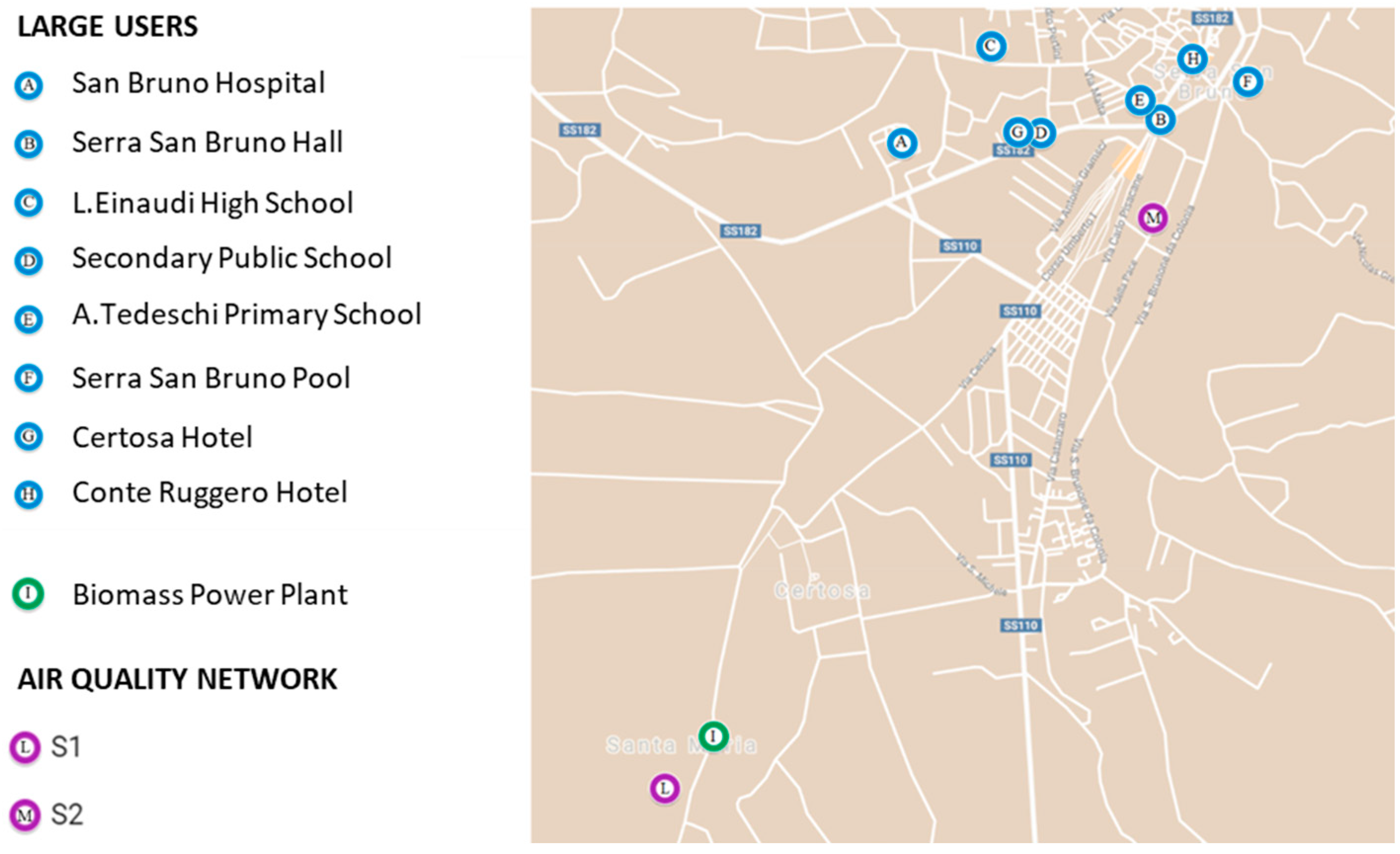
During the network design phase, the measurement systems were positioned in sensitive points of the considered area [19]. The first (S1), was positioned near the biomass power plant, while the second, (S2), was placed in the city center; Figure 2 shows their positions together with those of the major users considered.
3. Results
3.1. Estimated Consumption per Analogy
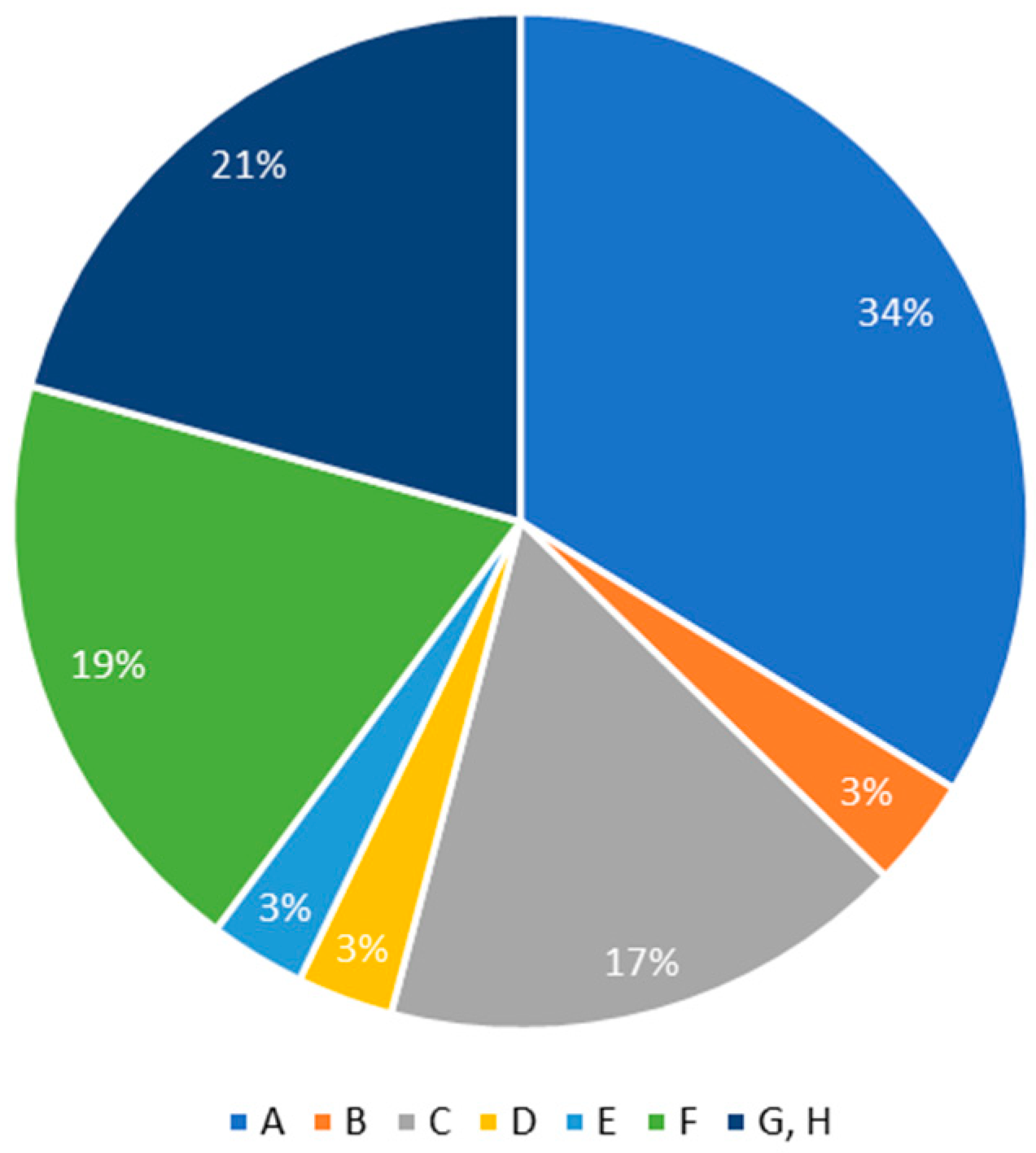
Energy consumption, as previously mentioned, was estimated for each large user by analogy with the structures reported in previous case studies. For user A, from the “Report on data collection for the determination and characterization of the types of systems for winter and summer air conditioning in hospital buildings” [20], which was drawn up by the ENEA, it is possible to obtain the total annual consumption per place and bed according to the size of the structure. From the data-set provided by the Italian Ministry of Health [21], it is possible to know the number of beds in the San Bruno Hospital, which is 34. Considering that the specific consumption for a hospital of this size is equal to 36,447 thermal kWh per year per bed, a total of about 1239 MWh/year is obtained. For user B, it is possible to make an analogy with a municipality with a population and average temperature similar to the one considered, and for which an energy diagnosis of the municipal building is available [22]. From the aforementioned energy diagnosis, the average consumption relating to the heating of the municipal building can be obtained, which is quantified at about 128 MWh/year. To obtain the information relating to the consumption of school users C-D-E, similar school structures with a comparable number of students and located in climatic conditions similar to the place considered were used as a reference. Considering the data reported in the APEA CT document [23], it is possible to estimate a consumption of about 617 thermal MWh/year for user C. From the energy census [24], it is possible to obtain a consumption of about 112 MWh/year for user D, and since user E is similar to D, it is reasonable to assume that the consumptions are similar and, therefore, also in this case equal to 112 MWh/year. The pool (user F) consists of five semi-Olympic lanes (length of 25 m). An energy audit is used as a reference relating to a plant that is similar in size to the swimming pools [25], from which a consumption of approximately 700 MWh per year is assumed. The energy consumption due to the heating of both hotels (users G and H) can be assimilated to those of a hotel for which data from an energy census carried out by APEA CT, already used previously, are available [23]. From the aforementioned energy census, data can be obtained regarding the heating needs for the reference hotel, which requires, on average, 379,32 kWh per year. Assuming that the two users G and H have a consumption, in thermal kWh/year, that equals double that of the hotel considered (reasonable hypothesis examining the number of rooms and floors of the buildings), it is possible to estimate the energy needs of both hotels of 759 MWh/year. The results are summarized in Table 3 and reported in Figure 3.
It is clear from Figure 3 that user A has the greatest thermal consumption at almost double that of user F, which is instead the second user for estimated consumption. The users C, G and H, representative of the school and the accommodation facilities, make a contribution that equals about 20% of the total, and therefore, almost comparable to that of user F. On the other hand, the consumptions due to users B, D and E are negligible. If considered individually, they consume about a tenth of the most energy-intensive structure (A) and represent just 3% of the total consumption considered.
3.2. Estimated Consumption with Coefficients
From a literature analysis, after taking into account the considered building area, it is possible to identify coefficients that allow us to obtain the annual thermal consumption. The coefficients were obtained from detailed energy analyses of structures that were used for the same purposes as those considered. In particular:
- For a hospital building (user A), a specific thermal consumption value of 15.93 thousandths of tons of oil equivalent (mTEP) per year per square meter was obtained, which is equal to approximately 185.3 kWh/m2 year [26];
- For primary and secondary schools (users D, E) a specific consumption, due to heating, of 130 kWh/m2 year was obtained [27];
- A value of 160 kWh/m2 year was obtained for a high school [27];
- For an outdoor swimming pool (user F) there is a specific consumption of 82 mTEP per year per square meter. However, this is due to both the heating and the electricity used. Assuming that the thermal rate is 50% of the total, a coefficient of 476.5 kWh/m2 year is obtained [28];
- The accommodation facilities (users G, H) and the municipal building (user B) share the same specific consumption as a house located in a climatic zone E (the same to which the municipality of Serra San Bruno belongs) with a high surface/volume form factor, i.e., 110 kWh/m2 year [29].
By multiplying the coefficients that were obtained for the considered area (Table 1), it is possible to obtain an annual thermal consumption value expressed in MWh/year. The results are summarized in Table 4.
To evaluate the domestic heating consumption, the residential buildings’ total area of Serra San Bruno was estimated; subsequently, we defined a specific average consumption per house, but only the quantity of energy used annually for heating was obtained. In particular, in the area considered, there are 2586 residential buildings, and the average surface area per dwelling is 97.4 m2 [30]. Furthermore, the data relating to the total area occupied by dwellings are directly known, which is equal to 244,460 m2 [30] (see Table 4). An intermediate specific thermal consumption value of 75 kWh/m2 year can be used, which is obtained from Annex C of D.Lgs 311/2006 [29], in which the limit values of the energy performance index for winter air conditioning are expressed. By multiplying this value by the total surface considered, an annual consumption of 18,334.5 thermal MWh is obtained (Table 4).
3.3. Comparison between Heat Consumption Estimated by Analogy and Obtained through Coefficients
By comparing the thermal consumption of large users obtained by analogy and those obtained considering a specific annual consumption per square meter of surface, it is possible to verify that the values belong to the same order of magnitude (Table 5). For further computations, the greater of the two values, or the more critical, will be taken into consideration.
3.4. Air Quality Analysis
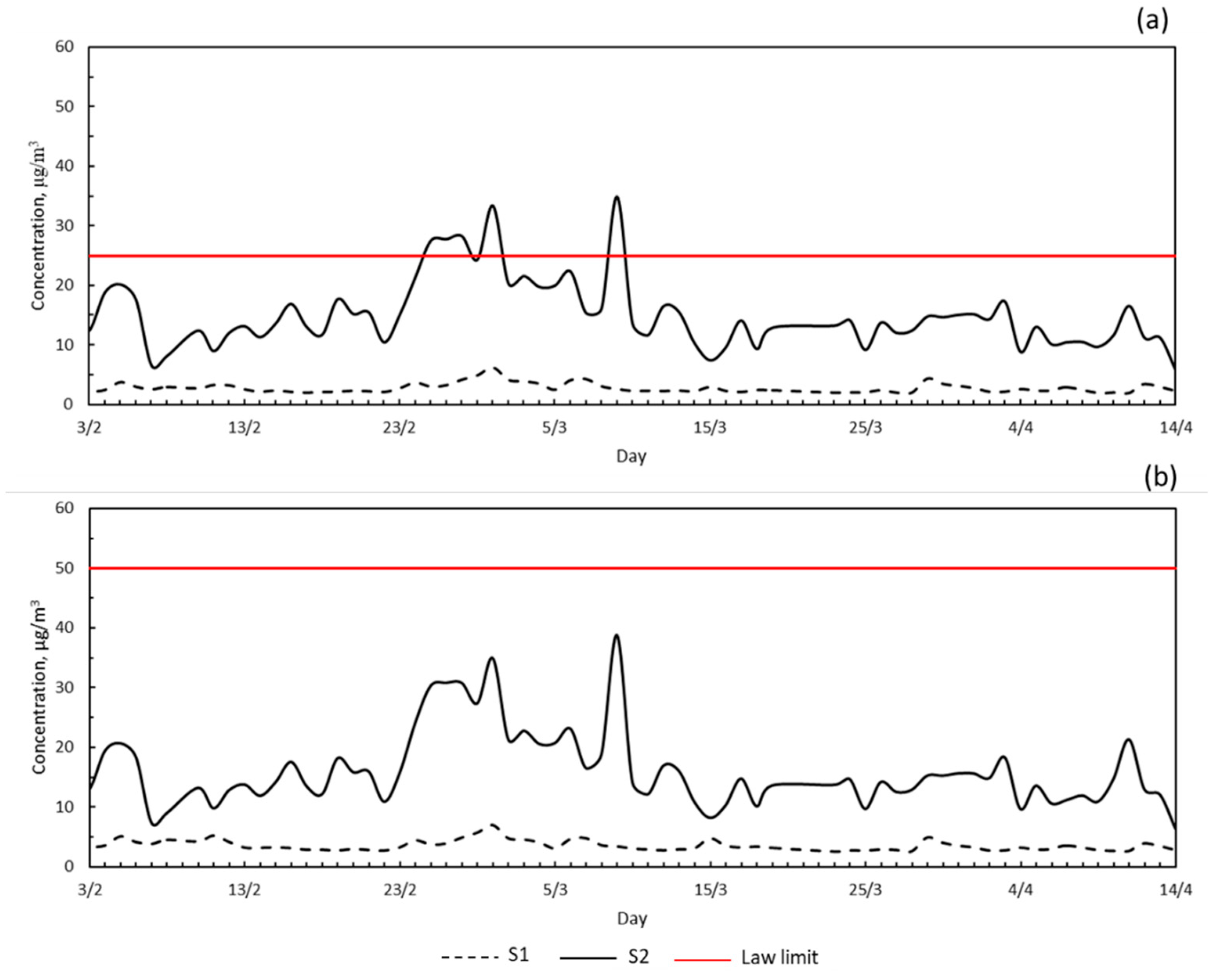
The values recorded by the S1 and S2 measuring devices are reported in Figure 4 and Figure 5, and for the period 1 February 2021–15 April 2021 as well as 16 April 2021–5 July 2021. The daily emission limit is represented by a red horizontal line and is 25 µg/m3 for PM2.5 and 50 µg/m3 for PM10. As can be seen from Figure 4 and Figure 5, the trend of average concentrations is similar for both PM10 and PM2.5 in the winter as in the summer. Only the concentration values vary, which appear to be slightly higher for PM10. However, this was predictable, since PM2.5 is a fraction of the latter.
It is important to highlight the presence of some peaks in concentrations during the winter period, for which values are very high from the average calculated previously. This led to the PM2.5 emission limit being exceeded, which was set at 25 µg/m3. These peaks occurred between 24th of February and 1st of March and 9th of March recorded by S2 (Figure 4).
Considering the average monthly temperatures of February and March, that are, respectively, 6.3 °C and 8.6 °C [31], it is found that the minimum measured is very close to them, in some cases even lower (for 01/03 and 09/03). In addition, 27th and 28th February are weekend days, leading to a greater presence of people inside their homes and, consequently, to an intensive use of heating. This means that it is possible to attribute the peaks in PM emissions largely to the prolonged use of domestic heating systems, with the other main source being vehicular traffic.
The pollutants’ dispersion is strongly influenced by meteorological phenomena; in particular, wind and rain can affect pollution levels. In the winter period there were about 25 days of rain, which corresponds to 35% of the period, while the wind had an average intensity of 7–35 km/h [31]. The rain and the high intensity of the wind certainly lowered the concentrations of airborne pollutants on some days, positively influencing the measurements. In different meteorological conditions, an increase in the concentrations of pollutants cannot be excluded. However, the introduction of the district heating system could mitigate this effect, offsetting the increase in pollutants due to stagnation.
With reference to the summer period, it can be noted that PM concentrations never exceed the law limit; in this case, values that differ slightly from the average value may be due to an intense presence of vehicles or fires. Another aspect to take into consideration is the considerable difference between the concentrations that was detected by the two different measuring devices, S1 and S2. This highlights that the quantity of pollutants emitted by the biomass power plant (measured by S1) is much lower than that measured in the inhabited center (measured by S2). This discrepancy is due to two factors, namely the presence of heating systems in the inhabited center and vehicular traffic. These elements do not influence the measurements of S1, as it is located in an area where there are no other buildings and far from main roads. On the contrary, S2 is located in the city center, therefore, it is in a very busy area with a high presence of heating systems.
3.5. Domestic Heating Contribution Evaluation
Starting from the values measured by S1 and S2, it is possible to calculate the average concentrations of PM2.5 and PM10 for the winter period (1 February 2021–15 April 2021) and the summer period (16 April 2021–5 July 2021); values are reported in Table 6. The winter period is characterized by the presence of domestic heating, while the summer period is characterized by the heating remaining switched off.
Assuming that vehicular traffic and any other sources that emit particulate matter contribute in the same way in both winter and in summer, the difference between the average concentration calculated in the winter and summer period represents the contribution due to heating of 7.7 µg/m3 for PM2.5 and 7.5 µg/m3 for PM10. Therefore, emissions due to heating comprise51% of the total PM2.5 emissions during the winter period, while those of PM10 are 46.5%.
To evaluate the impact due to domestic heating in relation to the particulate emissions into the atmosphere, the emissions of large users and residential buildings are evaluated by means of emission factors (Table 2, [18]). Finally, the weight of homes is evaluated in the PM issue. Given the characteristics of the area considered, the fuel used for heating homes is assumed to be 40% wood and the remaining natural gas [30], while for large users it is considered to be exclusively diesel. The estimated energy consumption and the relative PM10 and PM2.5 emitted are reported in Table 7.
It is, therefore, clear that homes account for 99.4% of particulate emissions due to heating. This result is not in line with the statistics published by ISPRA [32], according to which the residential sector is responsible for 64% of PM2.5 emissions, considering all sources. This contribution reaches about 76% if the rate due to productive activities is eliminated. This discrepancy may be because in the municipality in question, due to both its small size and mainly agricultural economy, there are fewer working activities than in other inhabited centers; another explanation could be found in the great difference between the fuels used by homes, with a quantity of wood very close to that of natural gas, and those used by the large users that were examined.
3.6. District Heating System Definition
It is possible to estimate the PM concentration variation if part of the utilities considered were converted to a district heating network. The presence of this system would entail the total replacement of the heating system currently present and, consequently, the emissions of particulate matter for the user considered.
Downstream of the analyses carried out in the previous sections, it is clear that, in the situation under consideration, the impact of homes is much greater than that of large structures: for this reason, the possible replacement of only domestic heating systems is considered. Due to the net losses caused by the distribution network, the biomass thermal conversion plant can deliver a power of 1 MW in the winter months (about 150 days), which translates into an energy equal to 3600 thermal MWh per year. They can be used, through district heating, in place of the energy that is generated by conventional domestic systems. In particular, two scenarios are considered:
- Fair replacement of wood and natural gas systems;
- Replacement of wood heating systems only.
3.6.1. Scenario 1
The contribution of the biomass power plant is removed half from the consumption that is due to wood-fired plants and half from those of gas plants. The results of this replacement are summarized in Table 8.
A decrease in PM10 concentration of 1.81 µg/m3 is obtained, while for PM2.5 the reduction is equal to 1.86 µg/m3.
3.6.2. Scenario 2
If the contribution of the biomass power plant is removed exclusively from the consumption linked to wood heating systems, the effects summarized in Table 9 are obtained.
This results in decreases in the concentrations of PM10 and PM2.5 of 3.6 µg/m3 and 3.72 µg/m3, respectively.
4. Discussion
The impact of heating (downstream of the considerations made) on PM emissions into the atmosphere is evident. In particular, about 50% of particulate pollution is attributable to it (51% for PM2.5, 46.5% for PM10).
It is also clear that the impact of a user does not depend exclusively on the amount of energy used, but also on the type of fuel used. This is the case of homes which, despite having an estimated consumption that is about 3.5 times that of all large users added together, weigh on particulate pollution for 99.4%. PM10 and PM2.5 emissions are practically entirely due to residential systems; in fact, it is verified that, of the 7.59 µg/m3 of PM2.5 due to heating in general, 7.54 µg/m3 derives from domestic heating systems. The reason for this high importance is not to be found only in energy consumption, which could be decreased by improving the thermal efficiency of the houses, but above all in the energy mix used (which was considered to be composed of 40% wood and 60% from natural gas).
The implementation of a district heating system, exploiting the heat of the fumes leaving the plant, could be particularly advantageous if it were carried out in a residential environment. This would allow the most to be made of the plant’s potential, which uses woody biomass, an energy source that is renewable and, if used correctly, carbon neutral. The district heating network would, therefore, make it possible to reduce the use of conventional heating systems, with a consequent decrease in particulate emissions. Specifically, if gas and wood-fired systems were to be replaced in equal measure, a reduction in the concentration of PM emissions due to heating would be obtained by approximately 24.5% (approximately one eighth of the total); if, on the other hand, only conventional heating systems that use wood were replaced, the decrease in the concentration of particulate emissions due to heating would be about 49% (about one eighth of the total). It is evident that wood, being a fuel with a very high PM emission factor, has a greater impact on particulate pollution. In fact, the decrease in concentration is significantly greater if they are eliminated, compatibly with the energy that the biomass power plant can only supply heating systems that use this energy source.
Furthermore, as shown in Figure 4 and Figure 5, the emissions of the thermal conversion plant are much lower than those due to the heating systems in the city center, even the net of the contribution of vehicular traffic.
Undoubtedly, since the construction of a district heating network is not without difficulties, other studies are needed to verify the actual benefits—not only environmental but also socio-economic—that the introduction of this system could entail.
Author Contributions
Conceptualization, N.L. and D.S.; methodology, N.L. and D.S.; software, N.L.; validation, N.L. and D.S.; formal analysis, N.L.; investigation, D.S.; data curation, N.L.; writing—original draft preparation, N.L.; writing—review and editing, N.L. and D.S.; visualization, D.S.; supervision, D.S.; project administration, D.S. All authors have read and agreed to the published version of the manuscript.
Funding
This research received no external funding.
Institutional Review Board Statement
Not applicable.
Informed Consent Statement
Not applicable.
Data Availability Statement
Not applicable.
Acknowledgments
The authors are very thankful to Aniello Di Giacomo for his helpful work.
Conflicts of Interest
The authors declare no conflict of interest.
References
- Shen, H.; Luo, Z.; Xiong, R.; Liu, X.; Zhang, L.; Li, Y.; Du, W.; Chen, Y.; Cheng, H.; Shen, G.; et al. A critical review of pollutant emission factors from fuel combustion in home stoves. Environ. Int. 2021, 157, 106841. [Google Scholar] [CrossRef] [PubMed]
- Hanigan, I.C.; Rolfe, M.I.; Knibbs, L.D.; Salimi, F.; Cowie, C.T.; Heyworth, J.; Marks, G.B.; Guo, Y.; Cope, M.; Bauman, A.; et al. All-cause mortality and long-term exposure to low level air pollution in the ‘45 and up study’ cohort, Sydney, Australia, 2006–2015. Environ. Int. 2019, 126, 762–770. [Google Scholar] [CrossRef] [PubMed]
- Apte, J.S.; Brauer, M.; Cohen, A.J.; Ezzati, M.; Pope, C.A. Ambient PM2.5 Reduces Global and Regional Life Expectancy. Environ. Sci. Technol. Lett. 2018, 5, 546–551. [Google Scholar] [CrossRef] [Green Version]
- Lotrecchiano, N.; Montano, L.; Bonapace, I.M.; Giancarlo, T.; Trucillo, P.; Sofia, D. Comparison Process of Blood Heavy Metals Absorption Linked to Measured Air Quality Data in Areas with High and Low Environmental Impact. Processes 2022, 10, 1409. [Google Scholar] [CrossRef]
- Varol, G.; Tokuç, B.; Ozkaya, S.; Çağlayan, Ç. Air quality and preventable deaths in Tekirdağ, Turkey. Air Qual. Atmos. Health 2021, 14, 843–853. [Google Scholar] [CrossRef]
- Sofia, D.; Coca Llano, P.; Giuliano, A.; Iborra Hernández, M.; García Peña, F.; Barletta, D. Co-gasification of coal–petcoke and biomass in the Puertollano IGCC power plant. Chem. Eng. Res. Des. 2014, 92, 1428–1440. [Google Scholar] [CrossRef]
- Magnani, F. Carbonio, energia e biomasse forestali: Nuove opportunità e necessità di pianificazione. For.-Riv. Selvic Ecol. For. 2005, 2, 270–272. [Google Scholar] [CrossRef] [Green Version]
- Sofia, D.; Giuliano, A.; Poletto, M.; Barletta, D. Techno-economic analysis of power and hydrogen co-production by an IGCC plant with CO2 capture based on membrane technology. In Computer Aided Chemical Engineering; Gernaey, K.V., Huusom, J.K., Gani, R., Eds.; Elsevier: Amsterdam, The Netherlands, 2015; Volume 37, pp. 1373–1378. [Google Scholar] [CrossRef]
- Bagaini, A.; Croci, E.; Molteni, T.; Pontoni, F.; Vaglietti, G. Valutazione Economica dei Beni Sociali dello Sviluppo del Teleriscaldamento; Bocconi Research Report N. 2; GREEN: Milan, Italy, 2020. [Google Scholar]
- Gong, M.; Zhao, Y.; Sun, J.; Han, C.; Sun, G.; Yan, B. Load forecasting of district heating system based on Informer. Energy 2022, 253, 124179. [Google Scholar] [CrossRef]
- Silveira, C.; Ferreira, J.; Monteiro, A.; Miranda, A.I.; Borrego, C. Emissions from residential combustion sector: How to build a high spatially resolved inventory. Air Qual. Atmos. Health 2018, 11, 259–270. [Google Scholar] [CrossRef]
- Assanov, D.; Zapasnyi, V.; Kerimray, A. Air Quality and Industrial Emissions in the Cities of Kazakhstan. Atmosphere 2021, 12, 314. [Google Scholar] [CrossRef]
- Zajacs, A.; Borodinecs, A.; Vatin, N. Environmental Impact of District Heating System Retrofitting. Atmosphere 2021, 12, 1110. [Google Scholar] [CrossRef]
- Haq, H.; Valisuo, P.; Kumpulainen, L.; Tuomi, V. An economic study of combined heat and power plants in district heat production. Clean. Eng. Technol. 2020, 1, 100018. [Google Scholar] [CrossRef]
- Sofia, D.; Giuliano, A.; Gioiella, F.; Barletta, D.; Poletto, M. Modeling of an air quality monitoring network with high space-time resolution. In Computer Aided Chemical Engineering; Friedl, A., Klemeš, J.J., Radl, S., Varbanov, P.S., Wallek, T., Eds.; Elsevier: Amsterdam, The Netherlands, 2018; Volume 43, pp. 193–198. [Google Scholar] [CrossRef]
- Lotrecchiano, N.; Sofia, D.; Giuliano, A.; Barletta, D.; Poletto, M. Real-time on-road monitoring network of air quality. Chem. Eng. Trans. 2019, 74, 241–246. [Google Scholar] [CrossRef]
- Sofia, D.; Lotrecchiano, N.; Trucillo, P.; Giuliano, A.; Terrone, L. Novel air pollution measurement system based on ethereum blockchain. J. Sens. Actuator Netw. 2020, 9, 49. [Google Scholar] [CrossRef]
- Virdis, M.R.; Gaeta, M.; Ciorba, U.; D’Elia, I. Impatti Energetici e Ambientali dei Combustibili nel Riscaldamento Residenziale; ENEA Report; ENEA: Rome, Italy, 2017. [Google Scholar]
- Sofia, D.; Lotrecchiano, N.; Giuliano, A.; Barletta, D.; Poletto, M. Optimization of number and location of sampling points of an air quality monitoring network in an urban contest. Chem. Eng. Trans. 2019, 74, 277–282. [Google Scholar] [CrossRef]
- Baldazzi, S.; Beltrone, E.; D’Alessandris, P.; Mostacci, A.; Mura, A.; Napoleoni, D.; Pasquino, F.; Santangelo, A.; Stemperini, A.; Toso, F. Rapporto Sulla Raccolta Dati per la Determinazione e Caratterizzazione Delle Tipologie di Impianto per il Condizionamento Invernale ed Estivo Negli Edifici ad Uso Ospedaliero; Report RdS/PAR2013/115; ENEA: Rome, Italy, 2014. [Google Scholar]
- Italian Ministry of Health. Posti Letto per Struttura Ospedaliera dal 2010 al 2019. Available online: https://www.dati.salute.gov.it/dati/dettaglioDataset.jsp?menu=dati&idPag=18 (accessed on 20 January 2022).
- Comune di Dorgali. Diagnosi Energetica di un Edificio; Comunali: Nuoro, Italy, 2007. [Google Scholar]
- Apea CT. Censimento Edifici 2013. Available online: http://censimento.apea.ct.it/edifici/edificio/087021_01 (accessed on 20 January 2022).
- VA17; Veneto Agricoltura; Natali, G. Diagnosi Energetica della Scuola Elementare Giovanni XXIII di Polverara (PD). Available online: https://www.venetoagricoltura.org/upload/audit%20energetico%20scuola%20elementare.pdf (accessed on 20 January 2022).
- Comune di Motta Visconti. L’audit Energetico degli Edifici e il Risparmio Energetico. Available online: https://www.comune.mottavisconti.mi.it/comune/documenti/libretto_audit_motta.pdf (accessed on 20 January 2022).
- Grassi, W.; Testi, S.; Menchetti, E.; Della Vista, D.; Bandini, M.; Niccoli, L.; Grassini, G.L.; Fasano, G. Valutazione dei Consumi Nell’edilizia Esistente e Benchmark Mediante Codici Semplificati: Analisi di Edifici Ospedalieri; Report RSE/2009/117; ENEA: Rome, Italy, 2009. [Google Scholar]
- Bianchi, F.; Altomonte, M.; Cannata, M.E.; Fasano, G. Definizione Degli Indici e Livelli di Fabbisogno dei vari Centri di Consumo Energetico Degli Edifici Adibiti a Scuole-Consumi Energetici delle Scuole Primarie e Secondarie; Report RSE/2009/119; ENEA: Rome, Italy, 2009. [Google Scholar]
- Santini, E.; Elia, S. Modello Matematico e Strumento Informatico User-Friendly per la Valutazione del Consumo e degli Interventi di Risparmio Energetico dei Centri Sportivi; RdS/PAR2014/080; ENEA: Rome, Italy, 2014. [Google Scholar]
- Decreto Legislativo 29 Dicembre 2006, n. 311. Available online: https://www.gazzettaufficiale.it/eli/id/2007/02/01/007G0007/sg (accessed on 20 January 2022).
- National Statistical Institute (ISTAT). Censimento Popolazione e Abitazioni. Available online: http://dati-censimentopopolazione.istat.it/Index.aspx (accessed on 20 January 2022).
- Climate Data. Dati Climatici Sulle città del Mondo. Available online: https://it.climate-data.org/ (accessed on 20 January 2022).
- Istituto superiore per la protezione ambientale. La Qualità Dell’aria in Italia; Edizione 2020; Istituto Superiore Per la Protezione Ambientale: Ispra, Italy, 2020. [Google Scholar]
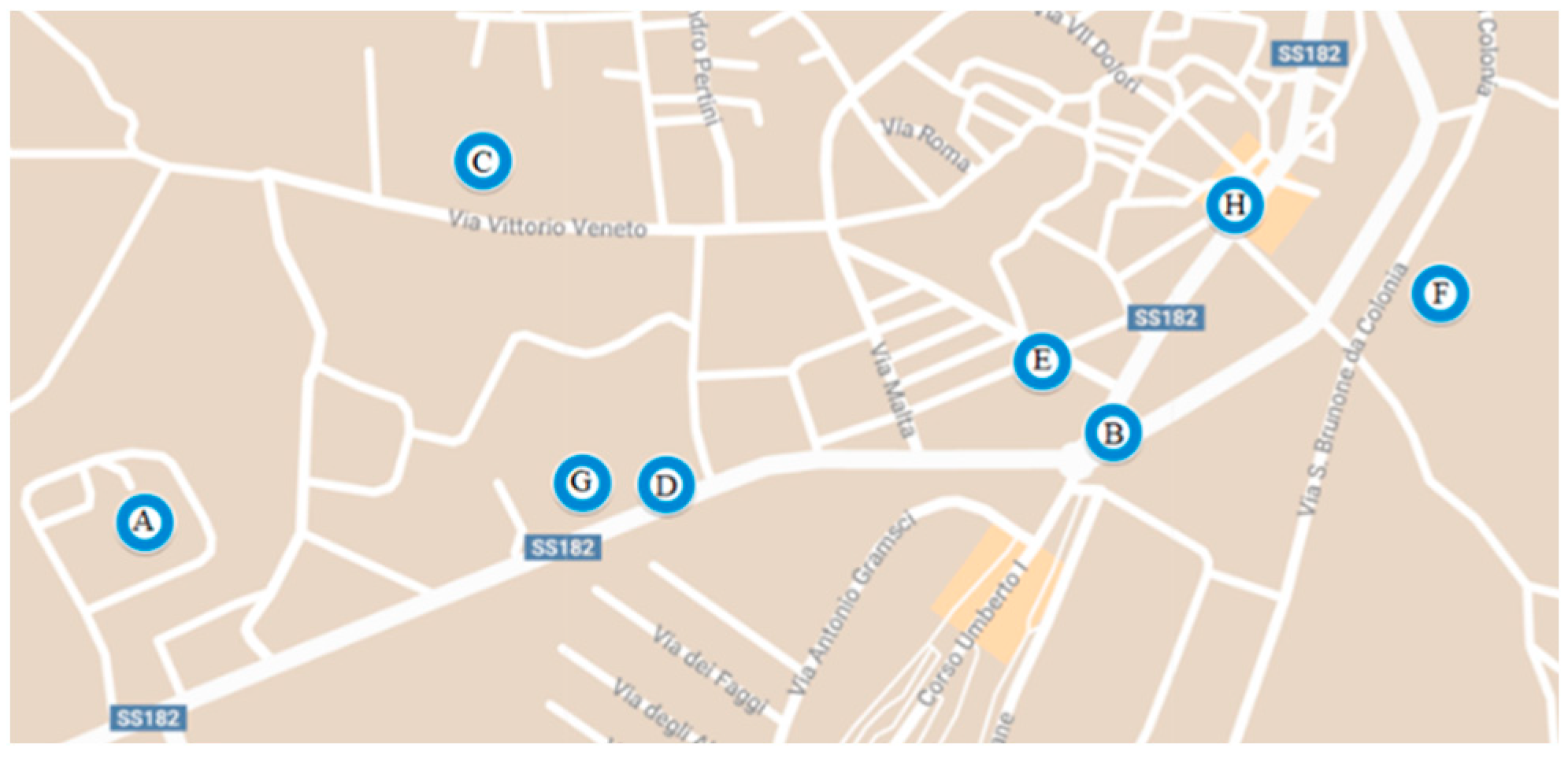
Figure 1.
Large users located in Serra San Bruno. (A) San Bruno Hospital, (B) Serra San Bruno Hall, (C) L.Einaudi High School, (D) Secondary Public School, (E) A.Tedeschi Primary School, (F) Serra San Bruno Pool (F), Certosa (G) and Conte Ruggero (H) Hotels.
Figure 1.
Large users located in Serra San Bruno. (A) San Bruno Hospital, (B) Serra San Bruno Hall, (C) L.Einaudi High School, (D) Secondary Public School, (E) A.Tedeschi Primary School, (F) Serra San Bruno Pool (F), Certosa (G) and Conte Ruggero (H) Hotels.

Figure 2.
Large users and air quality monitoring devices located in Serra San Bruno.

Figure 3.
Thermal energy consumption for the large users.

Figure 4.
Daily average concentration of (a) PM2.5 and (b) PM10 measured in S1 (black dashed line) and S2 (solid black line) in the period 1 February 2021–15 April 2021. Red solid line represents the law limit concentration for PM10 and PM2.5 according to D.Lgs 155/2010.
Figure 4.
Daily average concentration of (a) PM2.5 and (b) PM10 measured in S1 (black dashed line) and S2 (solid black line) in the period 1 February 2021–15 April 2021. Red solid line represents the law limit concentration for PM10 and PM2.5 according to D.Lgs 155/2010.

Figure 5.
Daily average concentration of (a) PM2.5 and (b) PM10 measured in S1 (black dashed line) and S2 (solid black line) in the period 16 April 2021–5 July 2021. Red solid line represents the law limit concentration for PM10 and PM2.5 according to D.Lgs 155/2010.
Figure 5.
Daily average concentration of (a) PM2.5 and (b) PM10 measured in S1 (black dashed line) and S2 (solid black line) in the period 16 April 2021–5 July 2021. Red solid line represents the law limit concentration for PM10 and PM2.5 according to D.Lgs 155/2010.


Table 1.
Large users characteristics.
| User | Total Area, m2 |
|---|---|
| San Bruno Hospital (A) | 12,387 |
| Serra San Bruno Hall (B) | 1312 |
| L. Einaudi High School (C) | 3224 |
| Secondary Public School (D) | 1870 |
| A. Tedeschi Primary School (E) | 1887 |
| Serra San Bruno Pool (F) | 1894 |
| Certosa (G) and Conte Ruggero (H) Hotels | 2304 |
Table 2.
Emission factors for domestic heating.
| Fuel | CO2 [kg/GJ] | CH4 [kg/GJ] | NOx [kg/GJ] | CO [kg/GJ] | NMVOC [kg/GJ] | SO2 [kg/GJ] | PM10 [g/GJ] | PM2.5 [g/GJ] |
|---|---|---|---|---|---|---|---|---|
| Coke | 105.93 | 0.015 | 0.07 | 5 | 0.005 | 0.682 | 439 | 219.5 |
| Steam coal | 91.66 | 0.2 | 0.05 | 5 | 0.2 | 0.646 | 439 | 219.5 |
| Wood | 92.71 | 0.32 | 0.06 | 5.39 | 0.638 | 0.013 | 403.9 | 400.2 |
| Diesel | 73.69 | 0.007 | 0.05 | 0.02 | 0.003 | 0.047 | 3.6 | 3.6 |
| GPL | 64.94 | 0.001 | 0.05 | 0.01 | 0.002 | - | 2 | 2 |
| Natural gas | 56.76 | 0.003 | 0.03 | 0.03 | 0.005 | - | 0.2 | 0.2 |
Table 3.
Thermal consumption estimated for the large users.
| User | Thermal Consumption Estimated, MWh/year |
|---|---|
| San Bruno Hospital (A) | 1239 |
| Serra San Bruno Hall (B) | 128 |
| L. Einaudi High School (C) | 617 |
| Secondary Public School (D) | 112 |
| A. Tedeschi Primary School (E) | 112 |
| Serra San Bruno Pool (F) | 700 |
| Certosa (G) and Conte Ruggero (H) Hotels | 759 |
Table 4.
Consumption due to heating considering the surface of the buildings.
| User | Total Area [m2] | Consumption [kWh/m2 year] | Consumption [MWh/year] |
|---|---|---|---|
| San Bruno Hospital (A) | 12,387 | 185.3 | 2295.3 |
| Serra San Bruno Hall (B) | 1312 | 110 | 144.3 |
| L. Einaudi High School (C) | 3224 | 160 | 515.5 |
| Secondary Public School (D) | 1870 | 130 | 243.1 |
| A. Tedeschi Primary School (E) | 1887 | 130 | 245.3 |
| Serra San Bruno Pool (F) | 1894 | 476.5 | 902.5 |
| Certosa (G) and Conte Ruggero (H) Hotels | 2304 | 110 | 253.4 |
| Domestic heating | |||
| Residential buildings | 244,460 | 75 | 18,334.5 |
Table 5.
Consumption due to heating calculated for analogy and considering the surface of the buildings.
Table 5.
Consumption due to heating calculated for analogy and considering the surface of the buildings.
| User | Consumption Estimated for Analogy, MWh/year | Consumption Estimated Considering the Surface, MWh/year | Critical Value, MWh/anno |
|---|---|---|---|
| San Bruno Hospital (A) | 1239 | 2295.3 | 2295.3 |
| Serra San Bruno Hall (B) | 128 | 144.3 | 144.3 |
| L. Einaudi High School (C) | 617 | 515.5 | 617 |
| Secondary Public School (D) | 112 | 243.1 | 243.1 |
| A. Tedeschi Primary School (E) | 112 | 245.3 | 245.3 |
| Serra San Bruno Pool (F) | 700 | 902.5 | 902.5 |
| Certosa (G) and Conte Ruggero (H) Hotels | 759 | 253.4 | 759 |
Table 6.
Average particulate matter concentration during the summer and winter period.
| Winter Period | Summer Period | |
|---|---|---|
| PM2.5 average concentration, µg/m3 | 15.0 | 7.3 |
| PM10 average concentration, µg/m3 | 16.0 | 8.5 |
Table 7.
PM10 and PM2.5 emissions for the large users and the residential buildings.
| User | Estimated Energy Consumption [MWh/year] | PM10 Emitted [kg/year] | PM2.5 Emitted [kg/year] |
|---|---|---|---|
| San Bruno Hospital (A) | 2295.3 | 29.75 | 29.75 |
| Serra San Bruno Hall (B) | 144.3 | 1.97 | 1.87 |
| L.Einaudi High School (C) | 515.5 | 8 | 8 |
| Secondary Public School (D) | 243.1 | 3.15 | 3.15 |
| A.Tedeschi Primary School (E) | 245.3 | 3.18 | 3.18 |
| Serra San Bruno Pool (F) | 902.5 | 11.7 | 11.7 |
| Certosa (G) and Conte Ruggero (H) Hotels | 253.4 | 9.84 | 9.84 |
| Total | 5206.5 | 67.48 | 67.48 |
| Residential buildings | |||
| Wood | 7333.8 | 10,663.64 | 10,565.95 |
| Natural gas | 11,000.7 | 7.92 | 7.92 |
| Total | 18,334.5 | 10,671.56 | 10,573.87 |
Table 8.
PM10 and PM2.5 emissions obtained by replacing wood and gas systems.
| User | Estimated Energy Consumption [MWh/year] | PM10 Emitted [kg/year] | PM2.5 Emitted [kg/year] |
|---|---|---|---|
| Wood | 5533.8 | 8046.4 | 7972.7 |
| Natural gas | 9200.7 | 6.62 | 6.62 |
| Total | 14,734.5 | 8053 | 7979.3 |
Table 9.
PM10 and PM2.5 emissions obtained by replacing wood and gas systems.
| User | Estimated Energy Consumption [MWh/year] | PM10 Emitted [kg/year] | PM2.5 Emitted [kg/year] |
|---|---|---|---|
| Wood | 3733.8 | 5429.08 | 5379.38 |
| Natural gas | 11,000.7 | 7.92 | 7.92 |
| Total | 14,734.5 | 5437 | 5387.3 |
Publisher’s Note: MDPI stays neutral with regard to jurisdictional claims in published maps and institutional affiliations. |
© 2022 by the authors. Licensee MDPI, Basel, Switzerland. This article is an open access article distributed under the terms and conditions of the Creative Commons Attribution (CC BY) license (https://creativecommons.org/licenses/by/4.0/).
Share and Cite
MDPI and ACS Style
Lotrecchiano, N.; Sofia, D. Analysis of the Air Quality of a District Heating System with a Biomass Plant. Atmosphere 2022, 13, 1636. https://0-doi-org.brum.beds.ac.uk/10.3390/atmos13101636
AMA Style
Lotrecchiano N, Sofia D. Analysis of the Air Quality of a District Heating System with a Biomass Plant. Atmosphere. 2022; 13(10):1636. https://0-doi-org.brum.beds.ac.uk/10.3390/atmos13101636
Chicago/Turabian StyleLotrecchiano, Nicoletta, and Daniele Sofia. 2022. "Analysis of the Air Quality of a District Heating System with a Biomass Plant" Atmosphere 13, no. 10: 1636. https://0-doi-org.brum.beds.ac.uk/10.3390/atmos13101636
Note that from the first issue of 2016, this journal uses article numbers instead of page numbers. See further details here.