Article

Machine Learning-Based Fog Nowcasting for Aviation with the Aid of Camera Observations

1
MicroStep-MIS, Čavojského 1, 841 04 Bratislava, Slovakia
2
Department of Astronomy, Physics of the Earth, and Meteorology, Comenius University Bratislava, Mlynská dolina, 842 48 Bratislava, Slovakia
*
Author to whom correspondence should be addressed.
Submission received: 8 September 2022 / Revised: 7 October 2022 / Accepted: 10 October 2022 / Published: 14 October 2022
(This article belongs to the Special Issue Decision Support System for Fog)

Abstract

:
In aviation, fog is a severe phenomenon, causing difficulties in airport traffic management; thus, accurate fog forecasting is always appreciated. The current paper presents a fog forecast at the Poprad-Tatry Airport, Slovakia, where various methods of machine learning algorithms (support vector machine, decision trees, k-nearest neighbors) are adopted to predict fog with visibility below 300 m for a lead time of 30 min. The novelty of the study is represented by the fact that beyond the standard meteorological variables as predictors, the forecast models also make use of information on visibility obtained through remote camera observations. Cameras observe visibility using tens of landmarks in various distances and directions from the airport. The best performing model reached a score level of 0.89 (0.23) for the probability of detection (false alarm ratio). One of the most important findings of the study is that the predictor, defined as the minimum camera visibilities from eight cardinal directions, helps improve the performance of the constructed machine learning models in terms of an enhanced ability to forecast the initiation and dissipation of fog, i.e., the moments when a no-fog event turns into fog and vice versa. Camera-based observations help to overcome the drawbacks of the automated sensors (predominantly point character of measurements) and the human observers (complex, but lower frequency observations), and offer a viable solution for certain situations, such as the recent periods of the COVID-19 pandemic.

1. Introduction

Fog, i.e., horizontal visibility below 1000 m on the ground [1] due to floating small water droplets in the air, is a hazardous meteorological phenomenon affecting various aspects of human life, from the safety of different ways of transportation (road, water, or air transport) to agriculture and tourism. In aviation, fog results in difficulties in landing/take-off, causes delays at airports, and generally, complicates the everyday work of air traffic controllers. Consequently, high-quality fog forecasting is also needed to more effectively plan airport routines, optimize flight diversions and additional fuel consumption, minimize economic losses, and just as importantly, reduce the inconvenience of passengers.
One of the most recent comprehensive overviews of the progress in the field of fog forecasting is the monograph chapter in a book by Koračin (2017) [2] (preceded by a similar review paper [3]). Even though the book is specifically devoted to marine fog, the reader can get acquainted with the evolution of various fog forecasting techniques, their conceptual differences, and their pros and cons, as well as the trends and the current challenges in fog forecasting.
In principle, fog can be forecasted by two conceptually different approaches. The first one is dynamic fog forecasting, in which the occurrence of the phenomenon is predicted on the basis of numerical weather prediction models (NWPs). Despite rapid improvements in the complexity of NWPs, the parametrization of the atmospheric processes/feedbacks involved, and the growing capacities of computational resources in the last few decades, the accurate forecasting of fog by means of NWPs still remains a huge challenge [4,5,6,7,8].
A significant supplement to the dynamic method is statistical fog forecasting, which has greatly expanded in recent years. Its basic process, in general, involves collecting a large set of meteorological variables (measurements or even NWP outputs) as potential predictors of fog, finding (by certain statistical tools) a limited number of significant predictors, and deriving (linear or non-linear) relationships to predict fog. Statistical fog forecasting models are computationally highly efficient; on the other hand, their validity is usually restricted to a limited site/area [2]. In the last couple of years, studies in statistical fog forecasting have been conducted, which make use of various machine learning (ML) algorithms. Without striving for completeness, these are, e.g., artificial neural networks [9,10,11], deep learning [12], feed-forward neural networks and tree-based ensemble approaches [13], random forests [14], decision trees [15,16], support vector machines [17], autoregressive time series analyses [18], and Bayesian decision networks [19]. Salcedo-Sanz et al. (2022) [20] presents a detailed review of the applications of ML methods in the statistical modelling of extreme meteorological phenomena, including fog. On top of these, the study of Castillo-Botón et al. (2022) [21] can be regarded as a benchmark in the field of statistical fog forecasting. They were the first in the literature to attempt to carry out an elaborate analysis of and test the performance of different ML algorithms for classification and regression problems. In regards to classification tasks (which is the core topic of the current study), they concluded that the most suitable methods were ensemble-based ones, such as random forest and gradient boosting techniques, since ‘learners are tree structures, which behave good for fog-events classification’ [21].
The efforts of our research team in the field of fog forecasting started with the study of Bartok et al. (2012) [22], which focused on the analysis of fog generation mechanisms, and particularly fog predictions on the north coast of the Arabian Peninsula, where the land–sea breeze circulation was found to be the specific climatic factor supporting fog generation. Their methodological approach consisted in the coupling of a one-dimensional PAFOG fog model [23] with a three-dimensional WRF 3.0 (Weather Research and Forecast, [24]) NWP system. The proposed method allowed for the construction of an efficient operative road traffic warning system for the occurrence of fog in the target region.
This fog prediction model was later further developed for the coastal desert area of Dubai, based on ML algorithms [16]. High-frequency observations from automatic weather stations were utilized as a database for the analysis of potential patterns. The inclusion of the decision trees approach for a lead time of six hours indicated a better model performance compared to that of the coupled WRF/PAFOG fog model from [22]. The results were further improved by integrating the output of the coupled numerical fog forecasting models into the training database of the decision trees.
In recent years, we have also adjusted the development of the fog forecasting models in our research group to the challenges of aviation meteorology and continued within the framework of the SESAR research projects [25]. A fog prediction model (with a lead time of 30 min and for a visibility below 300 m, as described in this study) was designed specifically for the systems of air traffic controllers to allow for the effective management of the queues of arriving and departing aircrafts (PJ.04-29.2, [26]). In parallel, the task ‘Remote Tower’ (PJ.05, [27]) was launched, which was related to the development of air traffic services by a remote air traffic controller, and this was followed by the task ‘Remote Observer’ (PJ.05-05, [28]) that focused on monitoring visibility, weather phenomena, and clouds by visual and infrared camera systems, with special attention given to inhomogeneous weather conditions.
During periods of bad weather, particularly in fog, airports may become completely invisible from the towers. In such cases, the control centers have to switch to radar and ‘low visibility procedures’ to ensure that airport operations can continue safely. These special procedures cover aircrafts upon approach and departure, as well as movements on the ground. In foggy conditions, aircrafts follow the instrument landing system (ILS) at airports to be automatically guided to the runway. After landing, an aircraft has to get far enough away from the runway such that it no longer interferes with the ILS radio beams before the next one can be given landing clearance. Aircrafts also have to be more widely spaced when maneuvering or taxiing. All these operations take extra time and they often result in considerable delays [29].
In aviation, an additional, visibility-based variable is defined, namely the runway visual range (RVR), which is the distance over which a pilot of an aircraft on the center line of the runway can see the runway’s surface markings delineating the runway and identifying its center line [30]. The RVR is used to support precision landing and take-off operations for aircraft pilots. The RVR, among others, determines local and international practices, such as airport operation categories (see an example in Table 1). Besides the main factor of visibility, the RVR is influenced by the runway lights’ intensity and background luminance. More intense runway lights increase the RVR, whereas low background luminance (cloudy sky, twilight) decreases it. Nevertheless, the most essential natural phenomenon that causes unexpected and significant degradation of the RVR is decreased visibility, which predominantly appears due to fog.
The current study was motivated by novel ideas in several directions. First, it was inspired by the ability of human aeronautical forecasters to accurately estimate approaching fog based on their visual perception of the fog and its time evolution in specific directions. Thus, a scientific question emerged on whether this knowledge could possibly be transformed into a ML predictor. Secondly, an automatic camera system for determining visibility for airports was developed within the above-mentioned SESAR project (PJ.05-05, [28]). Having installed this system at the Poprad-Tatry Airport in Slovakia, a very detailed database of omnidirectional visibility observations had become available. As a combination of the forecasters’ experiences and the technological developments, it was possible to construct a data mining model for forecasting fog, which was also based on predictors derived from the camera system beyond the ones from traditional meteorological observations.
The paper is structured as follows: After a description of the geographical/climatological settings of the target site (Section 2.1), the methodological approach to the analysis is described, which includes the principles of the camera-based remote observations (Section 2.2), the dataset (Section 2.3), and the data mining/machine learning methods (Section 2.4 and Section 2.5). The Results (Section 3) section starts with the long-term fog climatology, and continues with an analysis of the fog occurrence (types, frequencies, durations, etc.) on the basis of METAR messages (Section 3.1). Afterwards, the target attribute of the ML methods is defined (Section 3.2), and data-based (Section 3.2.1) and then figure-based analyses (Section 3.2.2) of the fog events are presented. The core of the modelling (Section 3.4) consists of two parts. First, the performances of the three selected ML methods are compared, and following this step, a detailed analysis of the various statistical scores related to the two best performing ML methods is carried out. The Discussion section attempts to put the results of the current study into a broader context (Section 4), and finally, the Conclusions section aims at summarizing the most relevant outcomes and possible pathways for the future development of the presented fog forecasting approaches (Section 5).

2. Materials and Methods

2.1. The Target Site and Its Climatology

The analysis focuses on a single target site, which is the Poprad-Tatry Airport (ICAO: LZTT, IATA: TAT). It is located in Northern Slovakia, at an altitude of 718 m above the sea level, which means that the LZTT is the highest elevated airport in the country, and one of the highest elevated airports for short- and medium-haul commercial aircrafts in Central Europe. The airport has one runway oriented in the east–west direction (09/27), of a dimension of 2600 m × 45 m. A significant feature of the airport is its geographical surroundings. The LZTT lies in the Poprad basin that is formed by the High Tatras Mountain (with peaks exceeding 2500 m) in the north, and the Low Tatras Mountain (with peaks up to 2000 m) in the south. In the west and east, the basin is open and without hills or obstacles.
The geographical settings of the LZTT significantly determine the local climatic conditions, mostly the wind speed and direction, and consequently, the occurrence of meteorological phenomena affecting aviation, such as turbulence, wind shear, fog, etc. Clearly, at the LZTT, the wind rose is dominated by the winds from the west: in about 30% (10%) of the cases, it blows from W (SW). The prevalence of the W and SW winds is underpinned by the fact that their average speed is about 4.5 m/s, whereas the wind speed averaged across all directions is 3.2 m/s (based on observations in the period 2001–2010 [31]). This average wind speed (3.2 m/s) is a typical value (between 2 and 4 m/s) for sites located in open basins in Slovakia [31]. Wind shear of orographic origin appears in the case of winds from the NW, N, or NE, while vertical rotors tend to occur on the luv side of the High Tatras.
The LZTT has a professional meteorological observatory, equipped with a standard automatic weather observation system (AWOS), and its professional observers regularly issue common meteorological messages, such as METAR. In the current study, we made use of the observations of meteorological variables at the LZTT from the period from January 2018 to March 2021, as this correlated with the availability of camera observations from the same site.

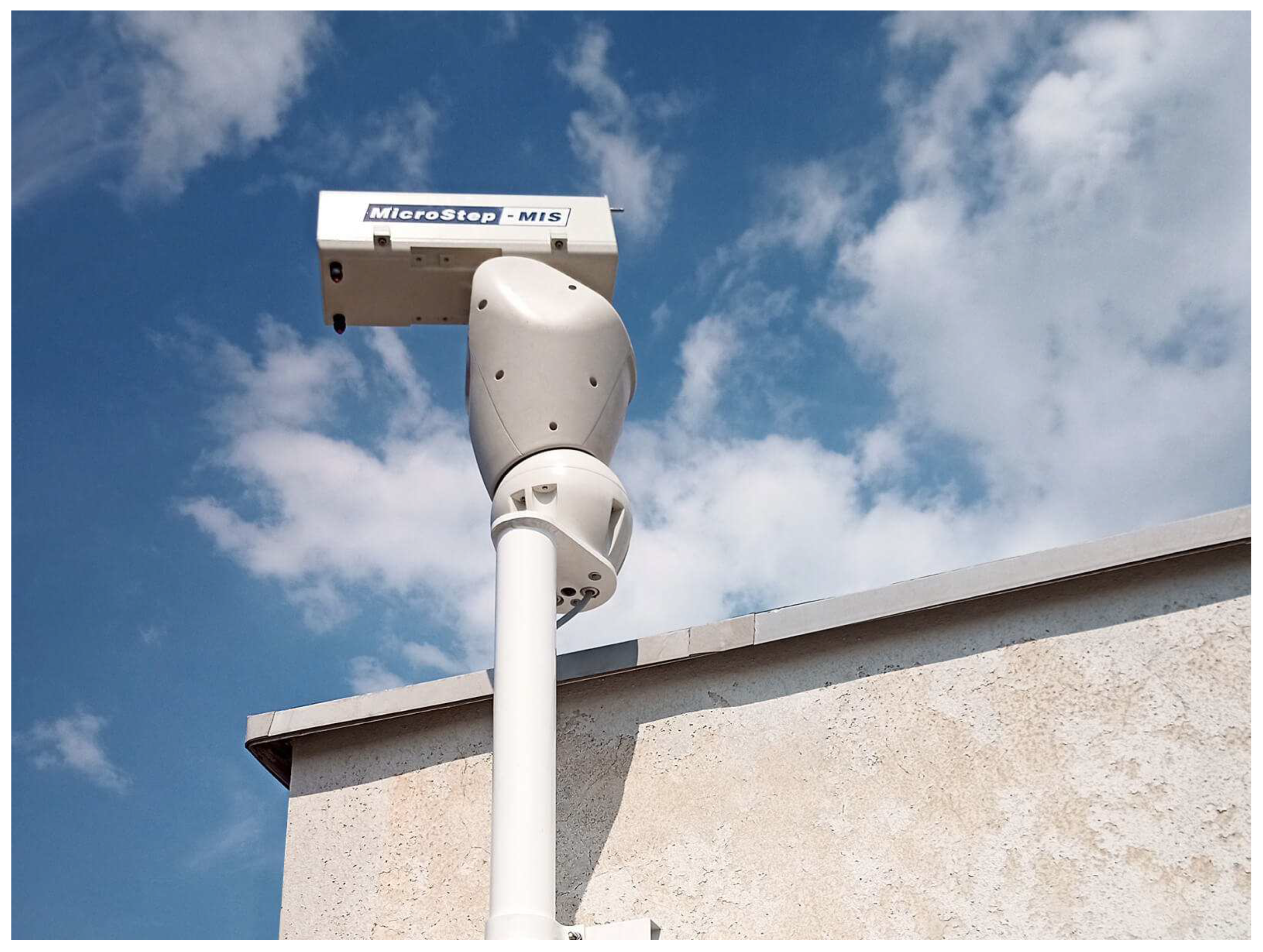
2.2. Camera-Based Observations of Visibility

There is a general tendency in aviation to automatize meteorological measurements as much as possible, with the aid of the AWOS. These are useful tools for the measurement of a wide variety of meteorological variables, mostly those that only require a specific, calibrated measurement device and in situations in which the subjective human decision procedure may completely be eliminated, e.g., air temperature, dew point temperature, pressure, wind characteristics, etc. Nevertheless, there are still a few variables that can be automatized with only a few compromises and that need complex human perception, e.g., in cases of estimating the prevailing visibility, cloud types/coverage, or occurrence of hazardous weather phenomena. Even though there are also efforts to replace these kinds of human observations with specific automated devices, one cannot disregard their universal drawback: they can only report point measurements, thus in the case of inhomogeneous weather conditions, the data provided by those sensors may not be representative for their entire surroundings.
This is exactly the case when the prevailing visibility is estimated, usually by one of the two types of automated devices: transmissiometers and forward scatter (FS) sensors [32]. Both types of sensors are generally designed to measure visibility by assuming that the conditions between the sensors’ receiver and transmitter represent the nominal conditions around the horizon. As the actual visibility may not be homogeneous over the entire domain (e.g., fog in patches), it is quite possible that the visibility estimates by the sensor at the point of its installation could differ from that of the human observer. A further major drawback related to automated visibility sensors is, in general, their inability to report the minimum visibility in specific directions required by the International Civil Aviation Organization (ICAO) [33].
A novel approach to the determination of visibility by remote and/or automatic means is using camera images. Cameras are generally available at affordable prices, even with programmable rotators included. Camera photos, in contrast to the visibility sensors, can cover the entire environment, and as a result of this feature, the minimum visibility and its direction can be determined in a relatively straightforward way.
Remote observations of visibility are carried out by means of a high-resolution camera for the visible spectrum that was installed at the LZTT at the location where the visibility for METAR messages is being regularly reported every half an hour by professional aviation observers. The camera installed on a rotator (Figure 1) sends eight images of the horizon covering all the cardinal directions (N, NE, E, SE, S, SW, W, and NW) to the central system. Each image has a full HD resolution, i.e., has a dimension of 1920 × 1080 pixels. For the current study, the target area was scanned by the camera at a 5 min interval.
The markers (landmarks) in all directions represent the cornerstone of the directional visibility estimation. These were selected carefully to cover the variability in the distances in each direction, and their distances to the observation point were measured using local maps of the airport and its surroundings. The number of markers was quite large, and thus, this made the estimation of the visibility more precise. Table 2 presents the basic statistics of the marker settings at the LZTT. The division of the markers into the distance categories was carried out according to the recommendations of the ICAO [33].
Figure 2 presents the spatial distribution of the markers in the vicinity of the LZTT, with a focus on the nearest ones within the two circles with radii of 0.6 and 1.5 km, corresponding to Table 2.
The basic principles of visibility estimation based on the set of markers assigned to the camera images are as follows:
  • If all the markers are visible in a given direction, then the visibility is larger than the distance of the most distant marker in this direction.
  • If some markers are not recognizable in a given direction, then the visibility is determined by the distance of the nearest visible marker preceding the first obscured one.
During nighttime, in accordance with the definition of the nighttime visibility by the ICAO Annex 3 [33], the camera observes visible lights (obstruction lights, buildings, street and highway lighting, etc.). Since the distances of these sources of lights are known, the same principles apply as in the case of the landmarks during the daytime.
All of these principles mimic the procedure that is followed by professional aeronautical observers.
The visibility from the camera imagery was determined manually by meteorologists, taking the above-mentioned principles into account.

2.3. Dataset

The initial dataset of observations at the LZTT originates from the period of January 2018–March 2021. One entry represents the whole set of observations for the given time. This includes:
  • information from the METAR messages available with a frequency of 30 min;
  • FS sensor measurements available with a frequency of 1 min, averaged through a 10 min moving window as per ICAO rules [33];
  • other AWOS sensor measurements at the same intervals;
  • camera imagery with frequency of 5 min supplemented by preceding sensor/camera measurements to these times.
Overall, 6.1% of the entries have no or some missing values. After removing the entries with missing/no values, 52,064 entries remained for modelling. A total of 1.7% (1.2%) of these are associated with a visibility lower than 1000 m (lower or equal to 300 m), which underpins the fact that the dataset is unbalanced from the point of view of the fog/no-fog ratio, and it needs to be resampled before adopting the ML procedures (Section 2.4.2).

2.4. Data Mining Methods

The goal of this study, i.e., developing a data mining method that can predict the occurrence of fog (class 1) and distinguish it from a no-fog event (class 0) in the near future, can be defined as a classification task. Common approaches are the classical rule-based methods [34] that rely on human expertise and machine learning methods [35] that rely on tagged datasets. Rule-based methods apply a set of rules derived by humans, such as ‘at Poprad-Tatry Airport, fog does not occur during the summer months at temperatures higher than 16 °C’, to a given input and reach a conclusion. These methods are easily interpretable and implementable; however, they might miss some of the insights gained by data mining. An update or a modification of rules can be easily implemented without the need to retrain the whole system. ML methods are less transparent, the quality of the predictions heavily depends on the quality of the dataset, and the implementation for production is less trivial; on the other hand, they are much better at recognizing patterns in data. ML methods range from easily interpretable decision trees to ‘black-box’ approaches, such as sophisticated deep learning methods. A methodically sound modelling protocol is essential for obtaining reliable outputs. It can help spot model flaws and detect irregularities in a given dataset. In order to update the ML model to account for additionally available data, retraining is necessary. Sometimes, a combination of rule-based and ML methods can significantly improve the results.

2.4.1. Rule-Based Methods in the Context of Unbalanced Datasets

It is known that classification problems in meteorology often involve unbalanced datasets [36]. In this case, it is not straightforward to implement a classification ML algorithm. One typically resamples the training dataset (so that the distribution of both classes is more balanced either by oversampling [37] or undersampling [38]), selects an adequate penalty function [39,40], or resorts to anomaly detection [41].
Since the aim of this study is to develop a generally applicable method for fog detection, undersampling was chosen because it reduces the existing bias towards the majority class. Undersampling describes a class of procedures that discard some of the dominant class samples (no-fog events) in order to improve the balance. In the current study, a rule-based method was applied, which systematically eliminated the no-fog events, based on a set of ‘IF-THEN’ rules collected by an expert.
Rule-based methods are expert systems that determine the outcome of a query, based on a set of rules called the ‘rule base’. A semantic reasoner reads in the input and evaluates the outcome based on the rule base by deciding which of the rules applies to the given situation and acting on it.
Utilizing the rule-based methods, a two-phase model was constructed:
  • Rule-based system: Based on the input features, determine whether one can safely conclude the occurrence of ‘no-fog’ event. If yes, end the task. Else, continue to step #2.
  • Machine learning classification: Based on the input features, predict the outcome (‘fog’ or ‘no-fog’).
The entire model of fog forecasting in the current study, described in detail in Section 2.3 and Section 2.4, is visualized in the form of a flowchart in Figure 3. The key element of the decision procedure is the above-described two-phase model of the prediction of ‘no-fog’ or ‘fog’ events.

2.4.2. Machine Learning Methods

There exists a wide range of ML methods used for classification tasks in weather forecasting [36]. In the following subsections, we briefly introduce the general features of the ones adopted in the current study. Further information on them (e.g., the most essential relationships) can be found in Appendix A.

K-Nearest Neighbors

The k-nearest neighbors algorithm (KNN; [42,43]) was originally developed in 1951 and can be used both for classification and regression tasks. It is a lazy supervised learning method. The algorithm can only be used with a labelled dataset. It is computationally cheap, because during the training phase, it simply stores the training dataset and does not perform any calculations. During the evaluation, the algorithm determines the distance between the data point being considered and all the stored training points in the feature space, selects k points, which are the ones nearest to the considered data point, and assigns a predicted label based on the majority vote. This algorithm is universally applicable since it makes no assumption about the data distribution and is well suited for pattern recognition. Its main disadvantages are the need to determine an optimal value of the neighbors, its sensitivity to irrelevant features, and a high likelihood of overfitting if many features are considered. Feature reduction either by a field expert or by automated feature reduction algorithms, such as a principal component analysis [44], is strongly encouraged.

Support Vector Machine

Support vector machine algorithms (SVM; [45]) were developed at AT&T Bell Laboratories in 1995. It is a class of supervised learning models with learning algorithms typically used for classification tasks, although suited for regression tasks as well. Each data point in the training dataset is plotted in an n-dimensional space, where n is the number of considered features. SVMs optimize the boundaries between the considered classes. These algorithms are effective in high-dimensional spaces and perform well even if the number of features is significantly larger than the number of samples. On the downside, these algorithms do not perform well with overlapping target classes.

Decision Trees

Decision trees (DTs; [46]) are a non-parametrical supervised learning algorithm, which can be used both in statistics and data mining. They can be applied both to discrete and continuous variables. During training, a DT searches for the most significant splitters, which can optimally divide the subset of the training dataset into several subsets. These algorithms are transparent, easily identify the most relevant features, can deal with different data types and noisy data, and make no assumptions about dataset distributions. Unfortunately, these algorithms tend to overfit. This can be remedied by using either an automatized or expert-based feature selection method. Therefore, in this study, an upper limit was set to the number of features (max. 20) considered at once in all ML models, including the DTs.

2.5. Verification Methodology

Generally, the success of ML highly depends on the settings of the training and testing processes. Our modelling process consists of six steps:
1.
Create a list of promising ML methods.
i.
For each ML method, create a list of hyperparameters.
The list should include ML methods suitable both from performance and deployment perspectives—accurate and fast enough, moderately computationally demanding, with modest memory requirements, etc. The corresponding hyperparameters can help in fine-tuning the performance of the methods. An example could be KNN with k = 3 or 5.
2.
Based on the available dataset, create systematic sets of features.
One should start by making a full list of available features, and subsequently, imposing restrictions, such as no more than a certain amount of N features at a time, to avoid overfitting. The generated subsets should each contain N or less elements. Another option would be to rely on expert knowledge/intuition and select elements based on rules.
3.
Split the dataset into training and testing parts.
It is a common practice to divide the dataset into two parts: the first one for training the ML models and the second one for testing their performance. In the current study, the data were randomly divided into two groups in a ratio of 70% for training to 30% for testing with a random seed, which ensured the reproducibility of the splitting.
4.
Loop over models, hyperparameters, and features:
i.
Train the model;
ii.
Evaluate the model.
In this step, the actual ML modelling was performed. The protocol can be best explained with a pseudocode:
   for model in models:
      for parameter in parameters:
        for set in features set:
          train model (parameter, set)
          evaluate model (parameter, set)
5.
Repeat steps #3 and #4 with different random splits.
Generally speaking, this step is optional. However, inspired by the statistical technique of bootstrapping [47], in order to obtain more accurate and robust results, the original dataset was resampled 200 times with the same ratio (70:30) and with random seed repetition.
6.
Evaluate the overall statistics.
In this step, the obtained results were analyzed. The overall statistical scores were calculated as the mean of the 200-model runs with different random seeds.
The performance of the forecast models, in general, is evaluated on the basis of the 2 × 2 confusion matrix (contingency table):
T N F P F N T P = c o r r e c t   n e g a t i v e s f a l s e   a l a r m s m i s s e s h i t s
where
  • TN is the number of cases, in which no fog was predicted and no fog occurred (true negatives or correct negatives or zeros);
  • FP is the number of cases with a fog forecast but fog did not occur (false positives or false alarms);
  • FN is the number of cases, in which no fog was predicted but fog occurred (false negatives or misses); and
  • TP is the number of cases, in which fog was forecasted and fog also occurred (true positives or hits).
The elements of the contingency table are then used for the definition of various scores giving detailed information about the statistical behavior of the examined forecast models. The most frequently used measures in atmospheric sciences are the probability of detection (POD) and the false alarm ratio (FAR). For rare events, such as fog, it is advised to use Gilbert’s skill score (GSS) and the true skill score (TSS) [48]. All of these can be complemented by the F1 score (F1), commonly used with ML processes, representing the harmonic mean of POD and precision (1 − FAR). Utilizing the elements of the contingency table (Equation (1)), these measures are defined as [49]
P O D = T P F N + T P = h i t s m i s s e s + h i t s
F A R = F P F P + T P = f a l s e   a l a r m s f a l s e   a l a r m s + h i t s
T S S = T N T P F P F N T N + F P F N + T P
G S S = T P T P r a n d o m T P + F N + F P T P r a n d o m
where
T P r a n d o m = T P + F N T P + F P T N + F P + F N + T P
F 1 = h i t s h i t s + 1 2 m i s s e s + f a l s e   a l a r m s = T P T P + 1 2 F N + F P
In addition to the above listed standard evaluation tools, it is interesting to track how good the models are at predicting significant changes. Therefore, we will try to evaluate, through an adequately defined metric, the per cent ratio of the correctly predicted fog starts (fog initiation) as well as the fog ends (fog dissipation). From a practical point of view, the metric related to the prediction of fog starts and ends is of particular importance in the everyday routines of air traffic controllers and airport staff.

3. Results

3.1. Statistical Analysis of Local Fog Patterns

Fog, i.e., when visibility drops below 1000 m [1], occurs at the LZTT, on average 52.1 days a year (1961–2010 [31]). Even though this is quite a substantial share of each year for airport operators and pilots to cope with consequences of fog, Poprad is classified in the set of Slovak stations with below-average values for the annual frequency of fog occurrence. A similar conclusion, although showing a slight increase in fog events in recent decades, was presented by Michalovič and Jarošová (2019) [50], who ranked the LZTT in third place among the four analyzed Slovak airports, in terms of their average annual fog occurrence (77.8 days), based on an analysis of METAR messages from the period 1998–2018. From a seasonal perspective, fog predominantly occurs during the autumn and winter seasons [31,50]. From the aspect of the diurnal cycle, most of the fog appears at night in the morning hours (between 12 p.m. and 12 a.m.)—this comprises 71% of all fog occurrences at the LZTT [50]. The annual and diurnal regime of fog occurrence in the target region is in line with the general features of its continental type of climate.
For the purposes of the current study, fog characteristics from the 39-month period (Section 2.3) were processed. Figure 4 shows the frequency of fog occurrence at the target site for the analyzed period, stratified according to hours of the day and the individual months. Herein, the observed low-visibility phenomena were classified as fog as soon as the METAR message reported: (i) visibility below 1000 m; and (ii) any type of fog. The figures in the matrix as well as the color shading of the cells in Figure 4 indicate the frequency of the occurrence of fog, expressed in the per cent of the total available number of METAR messages for the given hours and month.
Figure 4 clearly indicates that the most frequent occurrence of fog is associated with the cold half of the year, defined customarily as the period from October to March (though, in March, the fog occurrence is not significant). This is the main reason why the current study focuses on fog in cold seasons. From the perspective of the daytime occurrence of fog, Figure 4 reveals that fog at the LZTT typically occurs in the period from midnight to 8–9 a.m., which corresponds with the most intensive cooling of the Earth’s surface in the nighttime, and which is in line with the findings of the above-mentioned studies. The secondary maximum occurs in the late evening hours.
Table 3 ranks the fog types reported by professional meteorological observers in METAR messages that are issued each half an hour at the LZTT, according to their average annual frequency of occurrence. Note that the observers reported 20 further combinations of phenomena containing fog, but due to their low frequency of occurrence (less than three times per year), they were omitted from Table 3.
In METAR messages, fog (FG) is reported when the visibility drops below 1000 m [33]. Fog is classified as freezing fog (FZFG) when it consists of supercooled water droplets. Special cases of fog appear when the visibility inside the fog is less than 1000 m, but the visibility in the remaining sectors is 1000 m or higher. METAR messages distinguish the following special types of fog:
  • BC—fog patches randomly covering the aerodrome;
  • MI—shallow fog, reaching at most 2 m (6 ft) above ground level;
  • PR—partial fog, in which a substantial part of the aerodrome is covered by fog whereas the remainder is clear;
  • VC—fog in the vicinity, i.e., between the radii of approx. 8 and 16 km of the aerodrome reference point.
In cases, in which the visibility is at least 1000 m but not more than 5000 m, mist (BR) is reported in the METAR messages. Note that the abbreviation of ‘BR BCFG’ in Table 3 indicates the special case, in which patches of fog occur with a visibility inside them of less than 1000 m, but at the same time, the visibility in the remaining air space is between 1000 and 5000 m [33].
Unlike Table 3 which presents statistics related to the occurrence of different fog types in individual METAR messages, Figure 5 focuses on fog events. A fog event was defined by an uninterrupted sequence of fog reports in subsequent METAR messages. If, in a longer sequence of fog reports, even a single METAR message with no fog report was found, then the two parts of the sequence before and after the interruption were considered as two separate fog events.
Beyond the elementary finding that short fog events are significantly more frequent than the long ones, Figure 5 also indicates that the fog duration, in general, also depends on the fog type. Fog in patches (BCFG) rarely last longer than 4 h, whereas the duration of standard fog (and regardless of the air temperature, FG and FZFG) may exceed 10–12 h; in the outermost case, fog with a duration of 22.5 h was observed (not indicated directly in Figure 5, due to the scarce occurrence of fog events of longer durations). The average length of the BCFG (FG and FZFG) category was approximately 3.4 (7.5) METAR messages, i.e., 1.7 (3.8) h.
The presented analysis of the local fog patterns reveals that the fog in Poprad is of a local nature, with quite a patchy structure in time, and therefore, according to the analogy of Taylor’s hypothesis, also disjointed in space. This ‘non-continuous’ behavior classifies fog as a meteorological phenomenon that is rather hard to predict.

3.2. Target Attribute Definition

The variability of fog types, their occurrence, and/or the length of fog events indicated that the exact definition of the target attribute of the ML algorithms should be very carefully considered, i.e., which fog properties should be used for prediction. The decision procedure was mostly based on the following three findings:
  • The majority of fog occurs in the cold half of the year (Figure 4); thus, fog forecasting has the right justification in this time of the year;
  • The operationally significant visibility threshold for air traffic controllers and airport operators is 300 m (see ILS CAT II in Table 1; additionally, personal communication with several air traffic controllers);
  • On the basis of the METAR records, the number of events in the cold half of the year with a visibility below 300 m that were caused by meteorological phenomena not related to any type of fog was negligible. The detailed analysis of these low-visibility events revealed that they were exclusively caused by heavy snow, and consequently, they were excluded from the fog occurrences.
Having considered the above-listed facts, the dataset of meteorological observations at the LZTT was limited to the cold half of the year, and the binary target attribute was defined as follows:
  • ‘fog’ event (fog = 1/true) = when the 10 min running average of the visibility standardly available in METAR messages is less than or equal to 300 m;
Conversely:
  • ‘no-fog’ event (fog = 0/false) = when the 10 min running average of the visibility standardly available in METAR messages is higher than 300 m.

3.2.1. First Step of Modelling

The first task of fog modelling was to derive a set of rules for the rule-based step of our algorithm (Section 2.4.1) and prepare the undersampled dataset for the ML modelling that is required in its second step. This was carried out on the basis of the statistical distributions of the observed meteorological variables (extremes and selected quantiles of their distribution) and their relationship with the fog vs. no-fog events, as presented in Table 4.
The following meteorological variables were selected:
  • ws—wind speed in 10 m [m/s];
  • wg—wind gust in 10 m [m/s];
  • wd—wind direction in 10 m [degrees];
  • at—air temperature in 2 m [°C];
  • rh—relative humidity [%];
  • ap—atmospheric pressure [hPa];
  • ps—precipitation sum [mm/h];
  • sr—solar radiation [W/m2].
Note that wd is missing in Table 4 since fog occurred in connection with almost any wind direction, and this fact did not allow for the generation of a rule.
On the basis of the summary in Table 4, and also based on the expert knowledge of the long-term climatological conditions of the target region, the following conditions were defined as those favoring fog genesis at the LZTT:
  • ws: [0.2 m/s; 3.0 m/s]— neither wind calm nor strong wind support fog genesis;
  • wg: [0.3 m/s; 4.0 m/s]—the same reasoning as in the case of the common wind speed holds true;
  • at: [−14 °C; 16 °C]—considerably low air temperatures during the winter are associated with a low relative humidity; thus, no fog genesis is expected in such cases;
  • rh: [86%; 100%]— lower humidity favors no-fog;
  • ap: [920 hPa; 955 hPa];
  • ps: 0 mm/hr;
  • sr: [0 W/m2; 300 W/m2].
The decision algorithm, in accordance with the two-phase model described in Section 2.4.1 and Figure 3, can be formulated as follows:
  • IF all the above-listed seven conditions are met, keep the dataset sample and proceed to step #2 (ML classification);
  • ELSE discard the dataset sample and predict ‘no-fog’.
This algorithm has significantly reduced the initial dataset to the total number of 4214 entries potentially related to the occurrence of fog. Due to the applied rule-based model, the ratio of fog events, in which the visibility was ≤300 m (<1000 m), increased to 35% (47%), effectively balancing the dataset. Since the reduced dataset loses the character of the time series (as the remaining events are sparsely distributed in time), there is no need to account for the autocorrelation in later stages of the analysis [51].

3.2.2. Figure Based Analysis

Using camera imagery, one can gain deeper insight into the directional differences in the fog distribution as well as into the dynamics and temporal evolution of fog.
Figure 6, showing the situation on 17 October 2019 at 5:00 a.m., serves as an example of a spatially inhomogeneous fog event. As the camera records from different directions illustrate, the visibility is reduced in some directions (1.1 km NE, 1.5 km N), whereas in other segments of the horizon, the visibility is fairly good (7.5 km W). This kind of information on the spatial extent of the phenomena significantly differs from that obtained from the FS sensor (24,097 m in a 10 min average), which is only able to provide data of the point character.
Figure 7 demonstrates various stages of the morning fog approaching the airport on 17 October 2019. The sequence of records provides detailed information on the dynamics of the changes in the visibility in the given direction, which, in the presented example, changes from about 1500 m (at 05:20 a.m.) to about 50 m (at 06:05 a.m.).
Figure 8 presents the frequency distribution of the directions of the minimum visibility determined on the basis of the camera records. Low visibility at the LZTT tends to occur due to fog predominantly in southerly directions (S, SE, SW), whereas the second peak may be observed in the opposite directions (N, NW). Note that Figure 8 underpins the added value of the camera-based observations. Such a figure can be constructed neither on the basis of the METAR messages (since METAR contains information on the minimum visibility only in operationally significant cases; otherwise, only the prevailing visibility is standardly reported) nor based on the records of the FS sensor (since it only measures visibility at a fixed point).
The findings summarized in Figure 8 are best interpreted in light of Figure 9, which presents a composition of METAR-based wind roses for the target site from three different aspects. The first one (Figure 9, top) is the wind rose illustrating the wind conditions in Poprad for all climatology, i.e., for the entire analyzed period from January 2018 to March 2021, regardless of fog occurrence. This wind rose is fully in line with the overall wind climatology of the target site, also depicted in Section 2.1, with a dominance of winds from the W and SW, with an abundance of N and NW winds due to the blockage by the High Tatra Mountains, and with nearly the same mean (3.3 m/s) as for the average from the 2001–2010 period (3.2 m/s).
The remaining two wind roses are then directly related to the occurrence of fog, indicating the distribution of the wind speed and wind direction half an hour before fog onset (Figure 9, middle), and exactly at the time of fog onset (Figure 9, bottom), respectively. Both wind roses, according to expectations, show clearly decreased wind speeds in comparison with all climatology. Additionally, the distribution of the wind directions indicates a higher ratio of weaker winds from the southerly directions, which are also the directions with the highest frequency of the lowest visibilities, as illustrated in Figure 8.
Figure 6. Example of the records taken by the camera: directionally variable visibility at the LZTT on 17 October 2019 at 5:00 a.m.
Atmosphere 13 01684 g006
Figure 7. Example of the records taken by the camera: temporal evolution of fog in a fixed (Northern) direction on 17 October 2019.
Atmosphere 13 01684 g007
Figure 8. Distribution of the occurrence of the minimum visibility (below 300 m) in the cardinal directions, determined on the basis of camera records.
Atmosphere 13 01684 g008
Figure 9. Wind roses constructed on the basis of METAR messages for the entire period of January 2018–March 2021 (top), half an hour before fog onset (middle) and at the time of fog onset (bottom).
Atmosphere 13 01684 g009

3.3. Feature Selection

Since ML algorithms generally are sensitive to overfitting on a moderate-size dataset, the number of features entering the individual models should be low. Thus, the procedure of predictor selection started with the ‘basic’ variables from the set of AWOS measurements based on the judgement of meteorological experts: the hour of the day; month of the year; and the meteorological variables as listed in Section 3.2.1.
Subsequently, about 700 further derived predictors were constructed from these basic variables, mainly ‘delayed’ variables and ‘differences’. A delayed variable means that instead of the measured value at the time of the model run, an older value is used, e.g., relative humidity 5, 10, 15, … or 60 min before the model run time. Differences, on the other hand, indicate temporal changes in the basic variables (within the time window of 5, 10, 15, … 60 min). The working hypothesis was that the temporal changes could be important features for fog initiation. Nevertheless, the results did not meet these expectations. During the experiments, the performance of a multitude of various sets with the inclusion of the derived predictors (not more than a total of 20 predictors at once) was tested, but finally, the scores of the different ML models did not change significantly, only at the third significant figure (not shown). It was therefore concluded that the derived predictors were unimportant, except for those related to visibility. More specifically, each of the above-listed predictors (Section 3.2.1) should be used in the ML modelling with its value relating to the moment of the model run. The only exception is the visibility, which, beyond the time of the model run, is also significantly important 5 and 10 min earlier.

3.4. Machine Learning Performance

At this stage of the research, it was crucial to find out how the various ML methods perform in comparison to each other. To answer this question, an experiment was carried out, which was initialized with the same set of predictors for the entire set of ML methods, to examine the possible differences in their performances. The R [52,53,54] and PyTorch [55] libraries were used for implementation; their parameter/option settings can be found in Appendix A.4.
The results of this experiment are summarized in Figure 10, with the ML methods sorted in a descending order according to the POD values. In accordance with the findings of Lakshmanan et al. (2010) [56], the statistical scores of the various methods are generally quite similar: they are all able to detect the signal in the data. SVM exhibited the highest POD, followed closely by the DTs, with both methods having reasonably low FAR. KNN performed worse, but a trend can be distinguished, in which a higher number of neighbors leads to better results. On the other hand, a further increase in neighbors did not lead to a better performance; thus, the nine neighbors seem to be the optimum selection. The lowest value of the FAR is reached by the DTs, and with the second-highest POD value, this method seems to be suitable for decision support systems with a low tolerance for false alarms. All in all, the best results were reached by the SVM and DT methods, and consequently, a more elaborate analysis was dedicated to them.
Detailed results related to the different variants of the two best performing methods, SVM and DT, are presented in Table 5 and Table 6 and Figure 11. All of these outcomes are constructed on the basis of 200 resamplings, in which in each turn, 70% of the data was used to train the ML models, and the remaining 30% represented the verification dataset (Section 2.5). Table 5 and Table 6 present the average values of the resamplings, whereas Figure 11 allows for a deeper insight into the distributions of the selected major statistical scores.
Beyond the statistical scores POD, FAR, F1, GSS, and TSS, Table 5 and Table 6 involve two additional characteristics: FgIni and FgEnd, which were introduced especially for the purposes of the current study. The abbreviation FgIni stands for ‘fog initiation’, and it was defined to evaluate the successful prediction of the moments when a no-fog event ‘0’ changes to fog ‘1’, i.e., in terms of the target attribute, the visibility caused by fog decreases below the threshold of 300 m. Technically, FgIni is the number of successful predictions normalized by the total number of fog events. A similar line of reasoning also holds true in the opposite case: FgEnd (‘fog ending’ or ‘fog dissipation’ score) expresses the ratio of the successful forecast of the cases when a fog event ‘1’ changes to no-fog ‘0’, i.e., the visibility caused by fog increases above the threshold of 300 m. The values of these newly defined scores indicate the complexity and difficulty of the task of fog forecasting.
The analyzed variants of the SVM and DT methods differ from the perspective of the predictors included. In all of the ML variants, the core of the predictors consists of the same set of elementary meteorological variables, which are ws, wd, at, rh, ap, and ps. Nevertheless, more importantly, the individual variants of the ML models differ in terms of which of the three sources of visibility information they utilize. These are as follows:
  • the forward scatter sensor (vsFS), i.e., the visibility measured by the automated tool with a 1 min frequency (averaged through a 10 min window);
  • the METAR messages (vsMM), i.e., visibility determined by professional observers with a 30 min frequency;
  • the camera records (vsCR) with a 5 min frequency; more specifically, the minimum camera visibility constructed on the basis of the concurrent values from the eight cardinal directions.
Furthermore, as mentioned before, visibility data may also be used with a 5 or 10 min delay (D05/D10, i.e., earlier records) with respect to the model run-time. Note that the character of the ‘delayed’ variables (whether they are averaged or instantaneous) corresponds with their real-time counterparts. In other words, the variable vsFS-D05 (Table 6) is a 10 min average, since all the data from the forward scatter sensor are, in the very first step of the evaluation, averaged through a 10 min window. On the other hand, the variable vsCR-D10 (Table 5 and Table 6) is instantaneous, as it was derived from a still camera picture.
The traditional statistical scores (POD, FAR, F1, GSS, TSS) in Table 5 and Table 6 can be examined from several aspects. Firstly, the differences are small, and the models behave in a similar way. The variant DT #3 shows both the worst POD (0.84) and the best FAR value (0.22) among the analyzed ML variants (also in Figure 11). In terms of the F1 score, which combines all four elements of the confusion matrix (Equation 1), the best F1 score is associated with the DT #1 variant (again, see Figure 11). The TSS score values are quite similar in individual model groups, and are especially close in the SVM models.
As the figures in Table 5 and Table 6 indicate, the type of visibility data did not significantly affect the traditional statistical scores. On the other hand, the increase in the fog initiation score FgIni is noticeable from around 0.40 to 0.50 in the case of the SVM method and from 0.32–0.36 to 0.40 in case of the DT methods. The fog dissipation score FgEnd increased from 0.13–0.16 to 0.25 for the SVM method, and an even more remarkable increase was found for the DT method, from around 0.09 to 0.40. The presented figures underpin the importance of the camera system in the detection of changes in foggy situations. A deeper analysis related to these results is included in the Discussion section.
Concerning the selection of the optimal fog forecast model, the summary in Table 5 and Table 6 does not offer a straightforward guide but rather a set of recommendations for different decision support systems. Taking a holistic view of the traditional scores (F1, GSS, TSS), the best selection would be the DT #1 variant. Nonetheless, for a decision support system, the change scores FgIni and FgEnd may also be important since with changes in weather situations, the operative rules at the airport also change, and the system has to adapt to it, e.g., maintaining wider gaps between aircrafts when calculating the planes’ arrival and departure queues in fog. One may select either a model with higher fog initiation scores (FgIni = 0.50) but with the worst ability to predict the dissipation of fog (FgEnd = 0.25), which is the case of the variant SVM #3, or alternatively, one can select the DT #3 variant with levelled scores both for the initiation and dissipation of fog (equally 0.40 for both processes). The final choice should be governed by the preferences of the decision support system in the operative work. It can be based on an individual’s need, such as whether one prefers a more precise forecast of the beginning of an adverse weather event or a somehow balanced ability to predict both the start and the end of an unfavorable meteorological phenomena.
As an extension of Table 5 and Table 6, Figure 11 presents, in terms of box plots, some further properties of the distribution of the score values from the series of the resampling experiment (Section 2.5). Even though the box plots are restricted to the three most frequently used statistical scores, POD, FAR, and F1, it is obvious that they reproduce similar figures and overall, the same rankings of the individual ML variants as in Table 5 and Table 6. However, most importantly, the boxes are dense, indicating the low variability of each score; therefore, the average scores presented in Table 5 and Table 6 are robust and representative, and each of the resampled ML models is acceptably good.

4. Discussion

In the current paper, three different machine learning methods were adopted to predict the occurrence of fog in a short time horizon. The selection of the particular ML methods was partially influenced by the trends in the relevant and up-to-date research in the subject area; nonetheless, the scope of our methods could not be exhaustive. There is still a possibility to adopt further ML approaches, since any of the multitude of methods and/or configurations can lead to even a minor improvement in the statistical scores of the constructed models.
Herein, we attempt to compare the findings of our study with the baseline metrics. The first one is a simple fog forecast model based on the local fog climatology, i.e., using the knowledge of the long-term frequency of fog occurrence [51]. The second source of information is the ‘TREND nowcast’ message. These are special messages that are also issued by aviation forecasters; they follow the format of the TAF messages, but they are appended to the METAR messages. The results related to both approaches are summarized in Table 7. One can immediately see the poor performance of the climate-driven fog forecast model, which clearly confirms the unsuitability of using climate-type information in synoptic-type/local predictions in our target area. On the other hand, the quality of the fog predictions on the basis of the TREND nowcasts is higher. This is what currently is in operative use at the LZTT. From the aspect of FAR, the performance of the ‘TREND nowcast’ model is comparable with the SVM model variants (Table 5), but it does not reach the level of the DT variants (Table 6). In terms of the POD and F1, the ML models from Table 5 and Table 6 outperform the TREND message-based fog prediction model.
Since the cameras at the airport are a novel observation technique, it was not possible to find any study that analyzes the added value of the camera-based observations of visibility, which prevented us from evaluating the proposed camera-based approaches using some independent sources.
The trichotomy of visibility measurements and consequently, the construction of camera-based predictors are also worth a broader discussion. All of the three sources of visibility data have their pros and cons. The standard visibility sensors (used at the majority of airports globally) provide visibility measurements with a high frequency (~1 min) in an objective way; however, they characterize a localized point of the space, and therefore, they cannot principally distinguish directional changes in visibility and approaching fog. In contrast to this, METAR messages may contain detailed information on the directional visibility, since human observers are able (and have) to perform such observations. On the other hand, the frequency of METAR messages (30 min) may represent a serious issue in fog forecasting since significant changes in the fog density/structure may occur on smaller temporal scales. Cameras can distinguish directions and work operationally with a ~1 min frequency (though, we used a 5 min setting); thus, in this regard, they are possibly a valuable extension to the methods of observation by automated sensors and human professionals, at least in terms of the timings of fog initiation and dissipation.
Beyond the traditional statistical scores (POD, FAR, F1, GSS, ...), the special indicators FgIni and FgEnd (Table 5 and Table 6) were supposed to express the success of the predictions of the changes in the foggy conditions. The figures in Table 5 and Table 6 indicate that camera-based predictors indeed helped to increase the performance of the ML models, both in terms of the fog initiation score (FgIni) and the fog dissipation score (FgEnd). It is, therefore, worth of a closer examination of what is behind those findings. A schematic in Figure 12 was constructed to illustrate a typical situation at the airport with approaching fog.
Let us suppose that a cloud of fog is approaching the airport, but still has not reached it. At that moment, the meteorological variables at the airport are, generally, not able to indicate any discernible temporal change in the current weather (Section 3.3). On the other hand, based on camera records, one is able to recognize that fog is coming, i.e., fog is in the vicinity of the airport, but has not reached the area. Consequently, including the camera-based visibility as a ML predictor increases the performance of the ML models in forecasting the moments when the no-fog event turns into a fog event.
The procedure in the opposite direction, i.e., fog dissipation, seems to be more complex in comparison with fog initiation. The values of the FgEnd indicator are generally lower than those for the FgIni indicator (this also holds true for the variants of the ML approach without the camera-based predictors). This could be, in principle, explained by the fact that the FgEnd score comprises a superposition of two slightly different situations: (i) the camera is located entirely out of the fog; thus, it has the chance to ‘see’ the receding fog (which is exactly the inverse to the approaching fog); and (ii) the camera is covered by fog; therefore, it has limited ability to see the surroundings and to ‘help’ to the other predictors in the ML estimation.

5. Conclusions

In the recent years/decades, several studies worldwide (including the contributions of our research group to the topic) have confirmed that fog forecasting based on the various approaches of machine learning (ML) methods has potential. In particular, the transportation sector (road, air, or water) is probably the most affected by difficulties due to low visibility and the associated phenomena caused by fog (wet/slippery roads, freezing deposits, etc.). We limited our study to the field of aviation meteorology, in which the decision support systems of the air traffic controllers indeed need timely and accurate forecasting of any type of adverse weather phenomena, including fog at the airport. The innovation of the presented paper was the idea to use visibility information obtained from a camera system as a predictor in an ML-based fog forecast.
Observing systems with the use of cameras do not yet belong to the standard equipment in airport observatories. Their development for the purposes of aviation meteorology have just started recently, within the framework of several tasks of the manifold SESAR initiative [27,28]. Nevertheless, it is supposed that such observation systems capable of remote operation will expand in the coming years. A camera-aided system can qualitatively, objectively, and effectively complement standard meteorological observations [32]. Beyond helping to overcome the limitations stemming in the point character of the current automated measuring devices, these systems offer a viable option for professional observers to do their job remotely, e.g., from a distant airport, centralized office, or even from home. Remote observation gained more interest during the episodes of the COVID-19 pandemic, which forced both employers and employees to adapt to different levels of travelling restrictions or unprecedented living and working conditions.
In terms of traditional scores (POD, FAR, F1, etc.), the performance of the ML models was quite good, comparable to other approaches. One of the several positive findings of the current study is that the predictor constructed on the basis of the camera-based system is able to improve the forecast of both the start and the end of fog events (herein, when visibility drops below 300 m, or conversely, rises above this limit). This information is appreciated by air traffic controllers when scheduling special airport regimes in the case of the initiation or dissipation of fog. In a broader sense, more accurate fog predictions bring benefits for all participants in air transport: the passengers might not suffer from the consequences of delays and re-routed flights, the airlines may save fuel and additional costs, and overall, society as a whole may benefit from a higher level of air transport safety.
These first outcomes of the novel, camera-aided approach to fog forecasting are encouraging; however, further research is necessary to achieve more significant improvements in fog forecasting models. It is expected that in a time horizon of two to three years, the size of the available database of meteorological measurements will be doubled, which would naturally positively influence data-driven analyses. The same effect is anticipated by including further target sites into statistical fog modelling. From a long-term perspective, it would also be beneficial to extend the dataset of potential predictors with information derived from satellite imagery. Up to a point, satellite data are similar to those from the cameras: both offer a ‘visual’ view of the approaching/receding fog; however, due to the high local variability of fog, high-resolution satellite images should be used, such as those of the currently commencing METEOSAT Third Generation (MTG).
A further and important direction of future research will be to reach a phase of the automated recognition of visibility landmarks captured by cameras. In our research group, attempts have been made to use neural networks for the pattern recognition of visibility markers, and recently, deep learning algorithms are being implemented to boost the methods’ performance. To succeed in this challenge would be a step forward.

Author Contributions

Conceptualization, I.B. and J.B.; methodology, J.B., I.B. and I.M.O.; software, P.Š.; validation, P.Š., I.B. and I.M.O.; formal analysis, L.I.; investigation, P.Š.; resources, L.I.; data curation, L.I. and P.Š.; writing—original draft preparation, I.B., J.B., L.G. and I.M.O.; writing—review and editing, L.G. and J.B.; visualization, L.G.; supervision, J.B, L.G. and I.M.O.; project administration, L.I.; funding acquisition, J.B. All authors have read and agreed to the published version of the manuscript.

Funding

This work was supported by the Slovak Research and Development Agency under the contract no. APVV-20-0571 (ICONTROL) and by the SESAR Joint Undertaking under the European Union’s Horizon 2020 Research and Innovation Programme under the grant agreement No. 733121 (Solution PJ04-02: ‘Enhanced Collaborative Airport Performance Management’).

Institutional Review Board Statement

Not applicable.

Informed Consent Statement

Not applicable.

Data Availability Statement

Not applicable.

Acknowledgments

We would like to thank Martin Housa and the Department of Aviation Meteorology of the Slovak Hydrometeorological Institute for their support with the remote camera observations.

Conflicts of Interest

The authors declare no conflict of interest.

Appendix A. Basic Relationships and Settings of the Adopted Machine Learning Methods

Appendix A.1. K-Nearest Neighbors

The first step in the k-nearest neighbors algorithm is the determination of the distances between the evaluated instance and the instances in the training dataset, and subsequently, the selection of the k closest neighbors. Thus, a distance metric between the two feature vectors xi and xj should be defined. For an L-dimensional space of features, typically a special case of the Minkowski distance is chosen:
d M i n x i , x j = l = 1 L x i l x j l p 1 p
where the parameter p specifies the particular Minkowski space. If p = 2, we obtain the Euclidean distance:
d E x i , x j = l = 1 L x i l x j l 2
For p = 1, we obtain the Manhattan distance:
d M x i , x j = l = 1 L x i l x j l

Appendix A.2. Support Vector Machine

For linear separable data, support vector machines search for the best linear discriminator (a multidimensional hyperplane), which is located at the maximum possible distance from the planes of the training data. For a two-class classification, the training data can be represented as x 1 , y 1 , , x N , y N , where x i R L ,     y i 1 , 1 . The function of the linear discriminator is a hyperplane:
y x = w T x + b
where w is a weight vector and b is the shift of the hyperplane with regard to the origin.
The points closest to the separating hyperplane, satisfying y(x) = 1 or y(x) = −1 are called support vectors. The problem can thus be written as:
y i x i · w + b 1 0     for   i
The maximum distance to the hyperplane is equal to 1 w ; in other words, we are minimizing w . In general, the solution of this minimizing problem can be expressed as:
w = i = 1 N α i x i
where αi are optimization coefficients. Thus, the decision function can be written as:
y x = sign i = 1 N α i y i x · x i + b

Appendix A.3. Decision Trees

The iterative dichtomiser 3 (ID3, [57]) is one of the first and the simplest algorithms of the decision trees methodology. ID3 is a recursive algorithm, which chooses a feature for a root of the decision subtree for a set D with the largest information gain. The amount of information required to specify a class based on a selected feature can be described by the entropy H(D) or the information gain IG(α). Entropy describes the amount of uncertainty in the dataset D:
H D = c C p c log 2 p c
where C is the set of classification classes, p(c) the ratio of the instances belonging to class c to all instances in the dataset D.
The information gain IG(α) of the feature α is the difference in the entropies before and after the division of the set D based on this feature:
I G α = H D s S p s H S
where S is the disjunct set of instances created by dividing D based on the feature in such a way that their union is D.

Appendix A.4. Parameter/Option Settings for the Machine Learning Modelling

The following libraries were used in our implementation: kernlab [52], rpart [53], class [54] and PyTorch [55]. Unless specified otherwise, default parameter settings were adopted.
The parameters/options of the individual ML models were set as follows:
  • KNN—default values, number of neighbors varied depending on the model;
  • SVM—kernel = rbfdot (Radial Basis kernel ‘Gaussian’), type = C-svc (classification), C = 5 (regularization constant), sigma = 0.05 (inverse kernel width for the Radial Basis kernel function ‘rbfdot’ and the Laplacian kernel ‘laplacedot’);
  • DT—loss matrix = 0 1 1.5 0 , method = class (decision tree).

References

  1. WMO—World Meteorological Organization. Manual on Codes–International Codes, Volume I.1, Annex II to the WMO Technical Regulations: Part A Alphanumeric Codes; WMO–No. 306; WMO: Geneva, Switzerland, 2011; 480p. [Google Scholar]
  2. Koračin, D. Modeling and Forecasting Marine Fog. In Marine Fog: Challenges and Advancements in Observations, Modeling, and Forecasting; Koračin, D., Dorman, C.E., Eds.; Springer Atmospheric Sciences: Berlin/Heidelberg, Germany, 2017. [Google Scholar] [CrossRef]
  3. Koračin, D.; Dorman, C.E.; Lewis, J.M.; Hudson, J.G.; Wilcox, E.M.; Torregrosa, A. Marine Fog: A Review. Atmos. Res. 2014, 143, 142–175. [Google Scholar] [CrossRef]
  4. Wilkinson, J.M.; Porson, A.N.F.; Bornemann, F.J.; Weeks, M.; Field, P.R.; Lock, A.P. Improved Microphysical Parametrization of Drizzle and Fog for Operational Forecasting Using the Met Office Unified Model. Q. J. R. Meteorol. Soc. 2013, 139, 488–500. [Google Scholar] [CrossRef]
  5. Boutle, I.A.; Finnenkoetter, A.; Lock, A.P.; Wells, H. The London Model: Forecasting Fog at 333 m Resolution. Q. J. R. Meteorol. Soc. 2016, 142, 360–371. [Google Scholar] [CrossRef]
  6. Ducongé, L.; Lac, C.; Vié, B.; Bergot, T.; Price, J.D. Fog in Heterogeneous Environments: The Relative Importance of Local and Non-Local Processes on Radiative-Advective Fog Formation. Q. J. R. Meteorol. Soc. 2020, 146, 2522–2546. [Google Scholar] [CrossRef]
  7. Smith, D.K.; Renfrew, I.A.; Dorling, S.R.; Price, J.D.; Boutle, I.A. Sub-km Scale Numerical Weather Prediction Model Simulations of Radiation Fog. Q. J. R. Meteorol. Soc. 2021, 147, 746–763. [Google Scholar] [CrossRef]
  8. Boutle, I.; Angevine, W.; Bao, J.-W.; Bergot, T.; Bhattacharya, R.; Bott, A.; Ducongé, L.; Forbes, R.; Goecke, T.; Grell, E.; et al. Demistify: A Large-Eddy Simulation (LES) and Single-Column Model (SCM) Intercomparison of Radiation Fog. Atmos. Chem. Phys. 2022, 22, 319–333. [Google Scholar] [CrossRef]
  9. Colabone, R.O.; Ferrari, A.L.; Vecchia, F.A.S.; Tech, A.R.B. Application of Artificial Neural Networks for Fog Forecast. J. Aerosp. Technol. Manag. 2015, 7, 240–246. [Google Scholar] [CrossRef]
  10. Durán-Rosal, A.M.; Fernández, J.C.; Casanova-Mateo, C.; Sanz-Justo, J.; Salcedo-Sanz, S.; Hervás-Martínez, C. Efficient Fog Prediction with Multi-Objective Evolutionary Neural Networks. Appl. Soft. Comput. 2018, 70, 347–358. [Google Scholar] [CrossRef]
  11. Cornejo-Bueno, S.; Casillas-Pérez, D.; Cornejo-Bueno, L.; Chidean, M.I.; Caamaño, A.J.; Cerro-Prada, E.; Casanova-Mateo, C.; Salcedo-Sanz, S. Statistical Analysis and Machine Learning Prediction of Fog-Caused Low-Visibility Events at A-8 Motor-Road in Spain. Atmosphere 2021, 12, 679. [Google Scholar] [CrossRef]
  12. Zhu, L.; Zhu, G.; Han, L.; Wang, N. The Application of Deep Learning in Airport Visibility Forecast. Atmos. Clim. Sci. 2017, 7, 314–322. [Google Scholar] [CrossRef] [Green Version]
  13. Bari, D.; Ouagabi, A. Machine-Learning Regression Applied to Diagnose Horizontal Visibility from Mesoscale NWP Model Forecasts. SN Appl. Sci. 2020, 2, 556. [Google Scholar] [CrossRef] [Green Version]
  14. Benáček, P.; Borovička, P. Application of Machine Learning in Fog Prediction in the Czech Republic. Meteorol. Bull. 2021, 74, 141–148. (In Czech) [Google Scholar]
  15. Dutta, D.; Chaudhuri, S. Nowcasting Visibility During Wintertime Fog Over the Airport of a Metropolis of India: Decision Tree Algorithm and Artificial Neural Network Approach. Nat. Hazards 2015, 75, 1349–1368. [Google Scholar] [CrossRef]
  16. Bartoková, I.; Bott, A.; Bartok, J.; Gera, M. Fog Prediction for Road Traffic Safety in a Coastal Desert Region: Improvement of Nowcasting Skills by the Machine-Learning Approach. Bound. Layer Meteorol. 2015, 157, 501–516. [Google Scholar] [CrossRef]
  17. Negishi, M.; Kusaka, H. Development of Statistical and Machine Learning Models to Predict the Occurrence of Radiation Fog in Japan. Meteorol. Appl. 2022, 29, e2048. [Google Scholar] [CrossRef]
  18. Guijo-Rubio, D.; Gutiérrez, P.A.; Casanova-Mateo, C.; Sanz-Justo, J.; Salcedo-Sanz, S.; Hervás-Martínez, C. Prediction of Low-Visibility Events Due to Fog Using Ordinal Classification. Atmos. Res. 2018, 214, 64–73. [Google Scholar] [CrossRef]
  19. Boneh, T.; Weymouth, G.T.; Newham, P.; Potts, R.; Bally, J.; Nicholson, A.E.; Korb, K.B. Fog Forecasting for Melbourne Airport Using a Bayesian Decision Network. Weather Forecast. 2015, 30, 1218–1233. [Google Scholar] [CrossRef]
  20. Salcedo-Sanz, S.; Pérez-Aracil, J.; Ascenso, G.; Del Ser, J.; Casillas-Pérez, D.; Kadow, C.; Fister, D.; Barriopedro, D.; García-Herrera, R.; Restelli, M.; et al. Analysis, Characterization, Prediction and Attribution of Extreme Atmospheric Events with Machine Learning: A Review. arXiv 2022, arXiv:2207.07580. [Google Scholar] [CrossRef]
  21. Castillo-Botón, C.; Casillas-Pérez, D.; Casanova-Mateo, C.; Ghimire, S.; Cerro-Prada, E.; Gutierrez, P.A.; Deo, R.C.; Salcedo-Sanz, S. Machine Learning Regression and Classification Methods for Fog Events Prediction. Atmos. Res. 2022, 272, 106157. [Google Scholar] [CrossRef]
  22. Bartok, J.; Bott, A.; Gera, M. Fog Prediction for Road Traffic Safety in a Coastal Desert Region. Bound. Layer Meteorol. 2012, 145, 485–506. [Google Scholar] [CrossRef]
  23. Bott, A.; Trautmann, T. PAFOG—A New Efficient Forecast Model of Radiation Fog and Low-Level Stratiform Clouds. Atmos. Res. 2002, 64, 191–203. [Google Scholar] [CrossRef]
  24. Skamarock, W.C.; Klemp, J.B.; Dudhia, J.; Gill, D.O.; Barker, D.; Duda, M.G.; Huang, X.; Wang, W.; Powers, J.G. A Description of the Advanced Research WRF Version 3; (No. NCAR/TN-475+STR); University Corporation for Atmospheric Research: Boulder, CO, USA, 2008; 125p, NCAR Technical Notes 475. [Google Scholar] [CrossRef]
  25. SESAR Joint Undertaking. Available online: https://sesarju.eu/ (accessed on 22 August 2022).
  26. MET Performance Management. Available online: https://sesarju.eu/sesar-solutions/met-performance-management (accessed on 22 August 2022).
  27. Remote Tower. Available online: https://www.remote-tower.eu/ (accessed on 22 August 2022).
  28. Solution PJ.05-05 ‘Advanced Automated MET System’: TRL4 Data Pack. Available online: https://www.remote-tower.eu/wp/wp-content/uploads/2022/02/PJ05-05_TRL4_Data_Pack.zip (accessed on 22 August 2022).
  29. NATS–National Air Traffic Services. Available online: https://www.nats.aero/ (accessed on 26 August 2022).
  30. ICAO–International Civil Aviation Organization. Annex 6 to the Convention on International Civil Aviation—Operation of Aircraft. Part I—International Commercial Air Transport—Aeroplanes, 12th ed.; ICAO: Montreal, QC, Canada, 2022. [Google Scholar]
  31. Slovak Hydrometeorological Institute. Climate Atlas of Slovakia; Slovak Hydrometeorological Institute: Bratislava, Slovakia, 2015; 132p. [Google Scholar]
  32. Bartok, J.; Ivica, L.; Gaál, L.; Bartoková, I.; Kelemen, M. A Novel Camera-Based Approach to Increase the Quality, Objectivity and Efficiency of Aeronautical Meteorological Observations. Appl. Sci. 2022, 12, 2925. [Google Scholar] [CrossRef]
  33. ICAO–International Civil Aviation Organization. Meteorological Service for International Air Navigation. In Annex 3 to the Convention on International Civil Aviation, 17th ed.; ICAO: Montreal, QC, Canada, 2010. [Google Scholar]
  34. Grosan, C.; Abraham, A. Intelligent Systems: A Modern Approach; Springer Science & Business Media: Berlin, Germany, 2011. [Google Scholar] [CrossRef]
  35. Mitchell, T.M. Machine Learning; McGraw Hill: New York, NY, USA, 1997; 432p. [Google Scholar]
  36. Zeyad, M.; Hossain, M.S. A Comparative Analysis of Data Mining Methods for Weather Prediction. In Proceedings of the International Conference on Computational Performance Evaluation (ComPE), Online, 1–3 December 2021; pp. 167–172. [Google Scholar] [CrossRef]
  37. Chawla, N.V.; Bowyer, K.W.; Hall, L.O.; Kegelmeyer, W.P. SMOTE: Synthetic Minority Over-Sampling Technique. J. Artif. Intell. Res. 2002, 16, 321–357. [Google Scholar] [CrossRef]
  38. Barua, S.; Islam, M.M.; Yao, X.; Murase, K. MWMOTE—Majority Weighted Minority Oversampling Technique for Imbalanced Dataset Learning. IEEE T. Knowl. Data En. 2014, 26, 405–425. [Google Scholar] [CrossRef]
  39. Ting, K.M. A Comparative Study of Cost-Sensitive Boosting Algorithms. In Proceedings of the 17th International Conference on Machine Learning, Stanford University, Stanford, CA, USA, 29 June–2 July 2000; pp. 983–990. [Google Scholar]
  40. Jiang, L.; Li, C.; Wang, S. Cost-Sensitive Bayesian Network Classifiers. Pattern Recogn. Lett. 2014, 45, 211–216. [Google Scholar] [CrossRef]
  41. Goldstein, M.; Uchida, S. A Comparative Evaluation of Unsupervised Anomaly Detection Algorithms for Multivariate Data. PLoS ONE 2016, 11, e0152173. [Google Scholar] [CrossRef] [Green Version]
  42. Fix, E.; Hodges, J.L. Discriminatory Analysis. Nonparametric Discrimination: Consistency Properties. Int. Stat. Rev. 1951, 57, 238–247. [Google Scholar] [CrossRef]
  43. Altman, N.S. An Introduction to Kernel and Nearest-Neighbor Nonparametric Regression. Am. Stat. 1992, 46, 175–185. [Google Scholar] [CrossRef] [Green Version]
  44. Jolliffe, I.T.; Cadima, J. Principal Component Analysis: A Review and Recent Developments. Phil. Trans. R. Soc. A 2016, 374, 2015020220150202. [Google Scholar] [CrossRef] [Green Version]
  45. Cortes, C.; Vapnik, V. Support-Vector Networks. Mach. Learn. 1995, 20, 273–297. [Google Scholar] [CrossRef]
  46. Rokach, L.; Maimon, O. Data Mining with Decision Trees: Theory and Applications, 2nd ed.; World Scientific Pub Co., Inc.: Singapore, 2014. [Google Scholar] [CrossRef]
  47. Efron, B. Bootstrap Methods: Another Look at the Jackknife. Ann. Statist. 1979, 7, 1–26. [Google Scholar] [CrossRef]
  48. Marzban, C. Scalar Measures of Performance in Rare-Event Situations. Weather Forecast. 1998, 13, 753–763. [Google Scholar] [CrossRef]
  49. Wilks, D.S. Statistical Methods in the Atmospheric Sciences, 3rd ed.; Academic Press: New York, NY, USA, 2011; 676p. [Google Scholar]
  50. Michalovič, A.; Jarošová, M. Comparison of fog Occurrence at Slovak International Airports for the Period 1998-2018. In Studies of the Air Transport; Department of the University of Žilina: Žilina, Slovakia, 2021; Volume 10, pp. 159–162. [Google Scholar] [CrossRef]
  51. Vorndran, M.; Schütz, A.; Bendix, J.; Thies, B. Current Training and Validation Weaknesses in Classification-Based Radiation Fog Nowcast Using Machine Learning Algorithms. Artif. Intell. Earth Syst. 2022, 1, e210006. [Google Scholar] [CrossRef]
  52. Karatzoglou, A.; Smola, A.; Hornik, K. Kernlab: Kernel-Based Machine Learning Lab. R Package Version 0.9-31. 2022. Available online: https://CRAN.R-project.org/package=kernlab (accessed on 20 August 2022).
  53. Therneau, T.; Atkinson, B.; Ripley, B. Rpart: Recursive Partitioning. R Package Version 4.1-3. 2013. Available online: http://CRAN.R-project.org/package=rpart (accessed on 20 August 2022).
  54. Venables, W.N.; Ripley, B.D. Modern Applied Statistics with S., 4th ed.; Springer: New York, NY, USA, 2002. [Google Scholar]
  55. Paszke, A.; Gross, S.; Massa, F.; Lerer, A.; Bradbury, J.; Chanan, G.; Killeen, T.; Lin, Z.; Gimelshein, N.; Antiga, L.; et al. PyTorch: An Imperative Style, High-Performance Deep Learning Library. In Advances in Neural Information Processing Systems 32; Wallach, H., Larochelle, H., Beygelzimer, A., d’Alché-Buc, F., Fox, E., Garnett, R., Eds.; Curran Associates, Inc.: Red Hook, NY, USA, 2019; pp. 8024–8035. [Google Scholar]
  56. Lakshmanan, V.; Elmore, K.L.; Richman, M.B. Reaching Scientific Consensus Through a Competition. Bull. Am. Meteorol. Soci. 2010, 91, 1423–1427. [Google Scholar] [CrossRef]
  57. Quinlan, J. Induction of Decision Trees. Mach. Learn. 1986, 1, 81–106. [Google Scholar] [CrossRef]
Figure 1. Construction of the camera with the rotator.
Atmosphere 13 01684 g001
Figure 2. Spatial distribution of the markers with distance labels, used to identify directional visibility in the vicinity of the LZTT. (Map background: www.openstreetmap.org, accessed on 22 August 2022).
Atmosphere 13 01684 g002
Figure 3. Flowchart describing the entire procedure of fog forecasting, starting with the data collection and treatment of missing data, and the two-phase decision procedure that consists of the rule-based and machine learning methods. Abbreviations: AWOS—automated weather observing system; ML—machine learning.
Atmosphere 13 01684 g003
Figure 4. Frequency of fog occurrence, expressed as a per cent ratio of the total available number of METAR messages for the given hour (vertically) and month (horizontally) at the LZTT, in the period of January 2018–March 2021. Herein, the low visibility was declared as fog as soon as the METAR message included report of any type of fog and the visibility was below 1000 m.
Atmosphere 13 01684 g004
Figure 5. Histogram of the occurrence of fog events of different duration. Note that the duration is expressed in the unit of the frequency of METAR messages, i.e., in a ½ hour step. BCFG—fog in patches; FZFG and FG—freezing fog and fog with no further specification.
Atmosphere 13 01684 g005
Figure 10. Performance of different machine learning methods in terms of POD (probability of detection), FAR (false alarm ratio), and F1 (F1 score). The abbreviations of the models stand for: SVM—support vector machine, DT—decision trees, and 9NN/5NN/3NN—k-nearest neighbors (with numbers indicating the number of neighbors).
Atmosphere 13 01684 g010
Figure 11. Box plots of the distribution of three selected statistical scores of the models’ performance (POD—probability of detection, FAR—false alarm ratio, F1—F1 score), based on a validation experiment with 200 repetitions for each of the three variants of the SVM (support vector machine) and three variants of the DT (decision trees) methods. The box plots indicate the standard characteristics of the data distribution: median (middle line), the 25th and 75th percentiles (bottom and top edges of the boxes), the most extreme data points not considered outliers (whiskers), and the outliers (markers ‘o’).
Atmosphere 13 01684 g011
Figure 12. A schematic to illustrate the approaching fog (in the bottom right corner) at the airport. Green (red) markers indicate visible (invisible, fog-covered) landmarks. The position of the camera is indicated by the blue dot in the middle of the mesh of concentric circles.
Atmosphere 13 01684 g012
Table 1. Airport operation categories and the corresponding requirements for the minimum visibility in horizontal and vertical directions at a typical airport. Abbreviations: VFR—visual flight rules; ILS CAT—instrument landing system category; RVR—runway visual range; DH—decision height.
CategoriesMinimum Visibility [m]Height of the Lowest
Cloud Base > 4 Octas [ft]
VFR50001500
ILS CAT IRVR ≥ 550DH ≥ 200
ILS CAT IIRVR ≥ 300DH ≥ 100
ILS CAT IIIRVR ≥ 200DH < 100/no DH
Table 2. The number of landmarks used to identify directional visibility by the camera-based system at the LZTT. The original stratification by the ICAO distance categories was kept, but the first interval (0–600 m) was split in line with the settings of the current study.
Distance Interval [m]Number of Markers
0–30035
300–60021
600–150026
1500–500030
>500041
Total153
Table 3. Average annual frequency of occurrence of different type of fogs in METAR messages at the LZTT during the analyzed period of 3 and ¼ years. For a detailed explanation of the fog type codes, see Section 3.1.
RankFog Type—
Code
Fog Type—
Short Explanation
Annual Frequency
of Occurrence
1BCFGfog in patches225.5
2FZFGfreezing fog221.2
3FGfog with no further specification112.6
4MIFGshallow fog36.0
5PRFGpartial fog33.5
6VCFGfog in the vicinity24.6
7BR BCFGmist and fog in patches13.2
Table 4. Statistical characteristics (minimum, maximum, lower and upper 2.5% quantiles) of the selected meteorological variables influencing the occurrence of fog vs. no-fog events. Abbreviations: ws—wind speed, wg—wind gust, at—air temperature, rh—relative humidity, ap—atmospheric pressure, ps—precipitation sum, sr—solar radiation, min—minimum, max—maximum, q2.5%—the lower 2.5th quantile of the distribution, and q97.5%—the upper 2.5th quantile of the distribution.
No-FogFog
VariableMinq2.5%q97.5%MaxMinq2.5%q97.5%Max
ws [m/s]0.10.68.919.90.20.42.25.6
wg [m/s]0.10.911.224.10.30.52.88.4
at [°C]−22.8−9.714.033.2−14.4−10.812.915.9
rh [%]1036979986909999
ap [hPa]906.4919.6948.7962.0921.7923.4948.9953.0
ps [mm/hr]0001.50000
sr [W/m2]00824139200158296
Table 5. Average statistical scores (based on 200 resamplings) of three variants of the support vector machine (SVM) method. Abbreviations: POD—probability of detection, FAR—false alarm ratio, F1—F1 score, GSS—Gilbert’s skill score, TSS—true skill score, FgIni—fog initiation score, FgEnd—fog ending score, ws—wind speed, wd—wind direction, at—air temperature, rh—relative humidity, ap—atmospheric pressure, ps—precipitation sum, vsFS—visibility from the forward scatter sensor, vsMM—visibility from the METAR messages, vsCR—visibility from the camera records, and D05/D10—delay in minutes.
VariantPredictorsPODFARF1GSSTSSFgIniFgEnd
SVM #1ws, wd, at, rh, ap, ps, vsFS0.860.280.780.500.700.390.13
SVM #2ws, wd, at, rh, ap, ps, vsMM0.860.290.780.490.700.430.16
SVM #3ws, wd, at, rh, ap, ps, vsCR-D100.850.300.770.480.690.500.25
Table 6. The same as for Table 5, but for the three variants of the decision trees (DT) method.
VariantPredictorsPODFARF1GSSTSSFgIniFgEnd
DT #1ws, wd, at, rh, ap, ps, vsFS0.890.230.830.570.750.360.09
DT #2ws, wd, at, rh, ap, ps, vsFS-D050.870.230.810.550.730.320.08
DT #3ws, wd, at, rh, ap, ps, vsCR-D100.840.220.810.540.710.400.40
Table 7. Statistical scores of fog prediction models utilizing different inputs: fog climatology and TREND nowcast messages.
Fog Prediction ModelPODFARF1
fog climatology0.350.500.41
TREND nowcast0.680.310.69
Publisher’s Note: MDPI stays neutral with regard to jurisdictional claims in published maps and institutional affiliations.

