
Simulation of Air Pollutants Emission by Trucks and Their Health Effects

Department of Civil Engineering, Universidad Nacional de Colombia at Medellín, Calle 65 78-28, Building M1, Office 201, 050034 Medellín, Colombia
*
Author to whom correspondence should be addressed.
Atmosphere 2022, 13(10), 1691; https://0-doi-org.brum.beds.ac.uk/10.3390/atmos13101691
Submission received: 9 September 2022
/
Revised: 9 October 2022
/
Accepted: 12 October 2022
/
Published: 15 October 2022
(This article belongs to the Collection Measurement of Exposure to Air Pollution)
Abstract
:This paper analyzes the amount of truck emissions and their variations according to changes in travel schedules or routes and the impact on human health represented by cases of Acute Respiratory Infections (ARI) due to PM2.5 emissions in Medellín, Colombia. To accomplish this, information on each vehicle was collected, including model, year, type of fuel used, Euro, and engine power trucks. The commercial vehicles were equipped with GPS to obtain second-to-second speed, location, acceleration, and deceleration; the rest of the data were provided by the vehicles’ owners. All this information was used to estimate emissions with the HBEFA model. The main findings show a decrease of approximately 38% in emissions by changing the truck circulation schedule to off-hours and a generation of 2.35 annual cases of ARI if the amount of PM2.5 increases 1 μg/m3. Moreover, this investigation proposes that the optimal inter-city speed for truck circulation is between 40 km/h and 50 km/h, and it is recommended that some cargo transport operations should be carried out during off-hours, especially at night.
1. Introduction
Air pollution is the presence of toxic elements in the air that affect its normal composition and alter the constituent of the ecosystem [1]. According to their origin, pollutants are classified as anthropogenic, derived from human activity, or those derived from nature [2]. Furthermore, atmospheric pollutants are classified as primary and secondary. Primary atmospheric pollutants are those that remain in the atmosphere as they were emitted from the source, such as particles, carbon monoxide (CO), carbon dioxide (CO2), oxides of nitrogen (NOX), sulfur oxides (SOx), and hydrocarbons (HC) [3]. Secondary ones are those that have been subjected to chemical changes or the product of reactions of two or more primary pollutants in the atmosphere, such as sulfuric acid (H2SO4), nitric acid (HNO3), ozone (O3), photochemical smog, and compounds volatile organic compounds (VOC) [4].
The generation of polluting gases is congenital to any combustion process. However, the characteristics of the cycle used in the engine and the physical-chemical properties of the fuel directly influence the emissions that occur during operation [5]. Emissions related to the use of energy include emissions of CO2, methane (CH4), nitrous oxide (N2O), NOX, CO, volatile organic compounds other than methane (COVDM), and sulfur dioxide (SO2) emissions [6]. In combustion, there are several compounds, some of which are harmless and others toxic to human health; among the harmless are nitrogen (N), oxygen (O), CO2, hydrogen (H), and water vapor. However, the harmful ones include CO, HC, NOX, lead (Pb) and lead compounds, SO2, soot, and particulate matter (PM) [7]. Table 1 shows some pollutants, their health effects, and their emission origin.
Vehicles emit different pollutants into the atmosphere; the level of emission of these gases depends on the type of fuel used (gasoline, diesel, ACPM, natural gas vehicle (NGV)) and the state of the engine. The gear regime has a significant influence on the quantity and composition of the leaks, according to the type of circulation and topography of the land. Emissions from vehicles may be of polluting gases, evaporative emissions, and emissions from the exhaust pipe [8,9]. Freight vehicles mostly run-on diesel, which constitutes a mixture of various organic and inorganic substances in the form of gases and fine particles (composed of solid and liquid materials) [8,10]. Diesel emissions have significant quantitative differences, as illustrated in Table 2. The higher air/fuel ratio produces more complete combustion at higher temperatures with lower concentrations of carbon monoxide and hydrocarbons. However, they generate higher levels of NOX particles and sulfur compounds. Diesel engines of light vehicles emit approximately 50–80 times more particles than gasoline counterparts, and heavy ones generate 100–200 times more. However, the differences are decreasing with new engine models [10]. Table 2 shows the fuel types and their amount level of pollutants (concentration). Diesel fuel contains high levels of sulfur [11] and emits high levels of PM and SOX with respect to CO. Gasoline vehicles emit more CO pollutant.
Based on Table 2, to reduce sulfur levels in Diesel, a European standard on pollutant emissions was created [12]. The European standard is a set of requirements that regulate the acceptable limits for fuel gas emissions from vehicles that are in circulation. Selective catalytic reduction (SCR) is a system that reduces the emission of nitrogen oxides (NOX) and particles from the environment with the help of a reducing agent and a catalyst [13]. Current research [14,15] focuses on sustainability and the reduction of Green House Gas Emissions, among other important topics related to energy and pollution. Thus, it is important to have cutting-edge research to improve the living conditions in our countries. For example, in Colombia, Euro IV technology began in January 2015 [16], and the idea is to reduce emissions nationwide and, therefore, improve human health.
An increase in vehicular emissions deteriorates the air quality of metropolis cities. For example, in Madrid (Spain), the fleet cars contribute approximately 81.5% of the total undesirable compounds released into the atmosphere [2], an aspect that shows its importance compared to the other sources of pollution. In the case of Medellín city and its metropolitan area (Medellín Metropolitan Area (MMA)), transportation contributes 79% of the emissions, of which 49.8% of particulate matter (PM) is generated by trucks [17].
Most trucks are powered by diesel engines, which are very polluting due to their high sulfur content. This factor and others (e.g., emission technologies, vehicle age, and the weight of the load) affect the performance of the engine producing more emissions [18]. All these pollutants affect the environment, especially human health, contributing, for example, to respiratory diseases such as Acute Respiratory Infections (ARI) due to PM2.5 emissions. This topic has been deeply studied in developing countries [2]. However, the importance of the emissions in human health has not been studied in much detail in developing economies. Thus, the objective of this study is to know the variation in the number of emissions generated by trucks that circulate in urban areas due to the change in routes, which leads to a variation in the speed of circulation. To this effect, the authors collected information about truck circulation in urban areas during several hours of the day: conventional hours (HCON) and unconventional hours (HNC) using GPS technology. This information was the input to the Handbook Emission Factors for Road Transport (HBEFA) model to estimate the emissions according to vehicle circulation and operation parameters, among others, in the Medellín Metropolitan Area.
In Colombia and Latin America, Medellín is recognized as one of the cities with the highest pollution index [19]. This is mainly due to the topography (narrow and semi-closed valley). A city between mountains does not favor air circulation and hinders the dispersion of polluting gases [20]. Pollution levels exceed the standard established by WHO (PM2.5 10 μg/m3 annual average and 25 μg/m3 on average in 24 h; for PM10 20 μg/m3 annual average 50 μg/m3 on average in 24 h) [21] in Colombia, Resolution 2254 of 2017 governs which establishes as the maximum permitted levels of PM2.5 37 μg/m3 on an annual average and 25 μg/m3 on average in 24 h [22]. In Medellín, in the months of March and April, the permissible limits for both Colombia and the WHO standards [23] were due to weather conditions. The region has highly changing characteristics due to its tropical condition, orography, and high humidity availability which affects the dispersion in both the horizontal and vertical directions. Vehicular sources are the main cause of air pollution in Medellín because they emit 79% of the emitted gases [24]. The evidence found in the city ranges from measurements of environmental pollution levels in different areas of the Medellín Metropolitan Area (MMA), which is a region where Medellín is located with nine other municipalities. Until its relationship with respiratory problems [25,26,27], the evidence of these studies carried out in the city is based on the effect of pollution on human health [23].
Data from Air Quality Surveillance Network (Air network) [18,28] show that the daily, monthly, and annual averages of PM2.5 in most monitoring stations exceed the WHO standard. As mentioned earlier, vehicular sources emit 79% of emissions in MMA; that is, trucks emit 49.8% of PM2.5 emissions and 34.6% of NOX generated in MMA [24].
Trucks represent 4% of the total fleet of vehicles for 2015, and 86% of them use diesel fuel. However, this type of fuel is equivalent to 80.3% of PM2.5 and 68.5% of NOX of the total emission in MMA according to the inventory of emissions in 2015, when compared with Gasoline and Natural Gas Vehicles (NGV) [29].
Based on the above, it is necessary to know how the emissions are estimated, what quantity is estimated and what the behavior of truck emissions is. The main contribution of our paper is that we estimated emissions for commercial vehicles in a developing economy (Medellín, Colombia)—that was not performed before—and we found the relationship between Acute Respiratory Infections (ARI) and PM2.5 emissions, as presented below.
2. Materials and Methods
The methods described below explain the steps for estimating truck emissions on a given route in an urban area in the Medellín case study. The methodology could be applicable in urban areas like this city.
2.1. Base Information
In this process, primary and secondary information was collected. The primary information was collected with GPS on trucks that circulated in Medellín. The selected measurement equipment has been used in studies with trucks in New York, Santiago de Chile, Rio de Janeiro, Barranquilla, and Bogotá, among others, which is the GPS Columbus V-900. It is a data logger unit used to receive and record the geographical position and speed information second by second in an external memory card, saving the information in cvs format. To collect the data, the authors contacted different freight transport companies, which agreed that the drivers carry the GPS with them while driving. In this way, we could analyze the speed and driving cycles of the commercial vehicles. The secondary information was collected from the companies in which the tours were carried out. This information includes data related to the vehicle (model, year, type of fuel, Euro technology, engine power). This information was collected in order to estimate the emissions considering the characteristics of the vehicle.
The routes were selected based on the tours made by the companies. The analyses were conducted on those routes in both HCON and HNC to estimate the emissions of atmospheric pollutants. On the other hand, the GPS supplied in some trucks that circulated within the study area was used to analyze the cycle of conduction based on the geographical location and the second-by-second speed of the commercial vehicles.
Table 3 shows the vehicle characteristics considered in the selected routes. Heavy vehicles work with Euro VI [30]. The fact that vehicles use this Euro means that they emit a higher percentage of pollutant emissions into the atmosphere because they are an old version of Euro technology (IV) compared to the latest one (VI) that works worldwide [30].
2.2. Estimation of Emissions
For vehicle emissions, the Handbook Emission Factors for Road Transport (HBEFA) model (V3.2) was used (it does not measure emissions but estimates them). The HBEFA is a model that estimates emissions for all current categories of road vehicles (passenger cars, light vehicles, heavy vehicles, and motorcycles). In addition, it also estimates the emissions of some pollutants such as CO2, CO, NOX, HC, and PM2.5 [31], according to equation 1. HBEFA is used to estimate road transport emissions at different levels of space aggregation from the national level to the street level (route of a vehicle) [30]. The model was originally developed on behalf of the German Environmental Protection Agencies (UBA), Switzerland (FOEN/BAFU), and Austria (Umweltbundesamt). Meanwhile, other countries (Sweden, Norway, and France) and the Joint Research Center of the European Commission (JRC) support HBEFA [13,32,33]. The authors chose the HBEFA model because it is based on the Gaussian air pollutant dispersion model in the vicinity of linear emitters. The HBEFA emissions model was developed based on the results of exhaust gas measurements with dynamometric tests of light-duty vehicles (LDV) and heavy-duty vehicles (HDV), including dynamometric test measurements of LDV and HDV vehicles from real-world driving patterns. These procedures made it possible to obtain results that correspond to realistic traffic scenarios with the highest possible degree of accuracy [34].
HBEFA includes emission factors for vehicles of gasoline and diesel categories, with emission standards from EURO 0 to EURO 6. It has 272 traffic situations that are related to emission factors and fuel consumption for each vehicle segment and sub-segment. In addition, it considers the slope of the roads for values of −6%, −4%, −2%, 0%, +2%, +4%, +6%. Moreover, the model calculates fuel consumption and seven exhaust components (CO2, NOx, NO2, HC, CO, PM, PN) with the unit g/km for each of them [32,35]. The emission and fuel consumption of a vehicle depends on numerous parameters, such as the vehicle speed and load conditions, the longitudinal slope of the road, and dynamic driving parameters [36]. To describe the emission behavior of a vehicle, it is necessary to have information on emissions and fuel consumption for the typical driving patterns in real traffic situations. A driving pattern describes the course of speed over time (drive cycle), which tracks the driving behavior of a vehicle for a given driving situation, four of which are defined in HBEFA (“free flow”, “saturated traffic”, “heavy traffic”,“ Stop + Go ”) [32].
Equation (1) presents the HBEFA model.
where:
e = emission
v = Speed (m/s)
a = acceleration (m/s2)
ci= Calibration coefficients
The model estimates the emissions based on the speed, acceleration/deceleration of the vehicle in addition to the characteristics of the vehicle, such as the Euro technology used. The emissions estimated with the model are shown in detail from second to second, and the routes with higher emission percentages are presented. The coefficient values of the HBEFA model are presented in Appendix.
The customized procedure to estimate the emissions with the HBEFA model and see the effect of pollutants on human health in this research is as follows:
- Emissions estimation: Once the vehicles have been instrumented with the GPS, the information is extracted and processed to enter the data in the HBEFA model. To this effect, the information must be adjusted (units), that is, the GPS speed in km/h, the speed in m/s, and additionally, it is necessary to calculate the acceleration of the vehicle during the journey. The model must be adjusted according to the characteristics of the vehicle, knowing the type of truck and the EURO technology. With this, the emission of CO2, CO, NOx, HC, and PM2.5 is estimated.
- The routes are loaded with the emissions in GIS software, and the routes are drawn to know the critical areas of the study area.
- Analyze the literature to know the emission range in which a person can experience a health problem due to some type of pollutant and what diseases they can manifest.
- Information from the department of health is analyzed to seek the zones with the highest levels of pollution and people from those zones that present cases of ARI disease.
- Obtain the costs generated by the diseases caused by the different pollutants in people and thus know the economic value of this.
- Different scenarios must be analyzed, that is, routes in HCON and HNC, to make a comparison of the emissions generated at different times.
2.3. Change of Circulation Schedule
After having emissions of air pollutants in conventional hours HCON (scheduled between 06:00 and 18:00), emissions were estimated in unconventional hours HNC (between 18:00 and 06:00) of the following day to analyze the behavior of the emissions in the two periods of time and to define if changing the circulation schedule influences decreasing the amount of air pollutants.
3. Results
The emissions of a lot of routes were estimated. For illustration purposes, only a sample of five routes is presented. These routes were selected considering the main roads of the city. The type of trucks used in the routes were small trucks with two axles.
Table 4 shows a summary of the information provided by the GPS. The information obtained was the second-to-second speed and acceleration, and it allowed the authors to estimate the emissions. The tours were made during the daytime, which started and ended in the same place between 06:00 and 14:00. Full-cycle tours were made, and the average tours had a median duration of 8 h, as shown in Table 4. The average speed of the routes was 20 km/h, which shows that the city of Medellín is congested. Thus, it is implied that the studied trucks produce higher levels of air pollutants than in free-flow or uncongested conditions. For these commercial vehicles, it is necessary to improve their technology to have better results as regards the emission. These vehicles currently produce 580 Ton/year of PM2.5, according to the AMVA 2015 emissions inventory. In this city, there are approximately 1,200,000 vehicles, of which 27,000 are trucks.
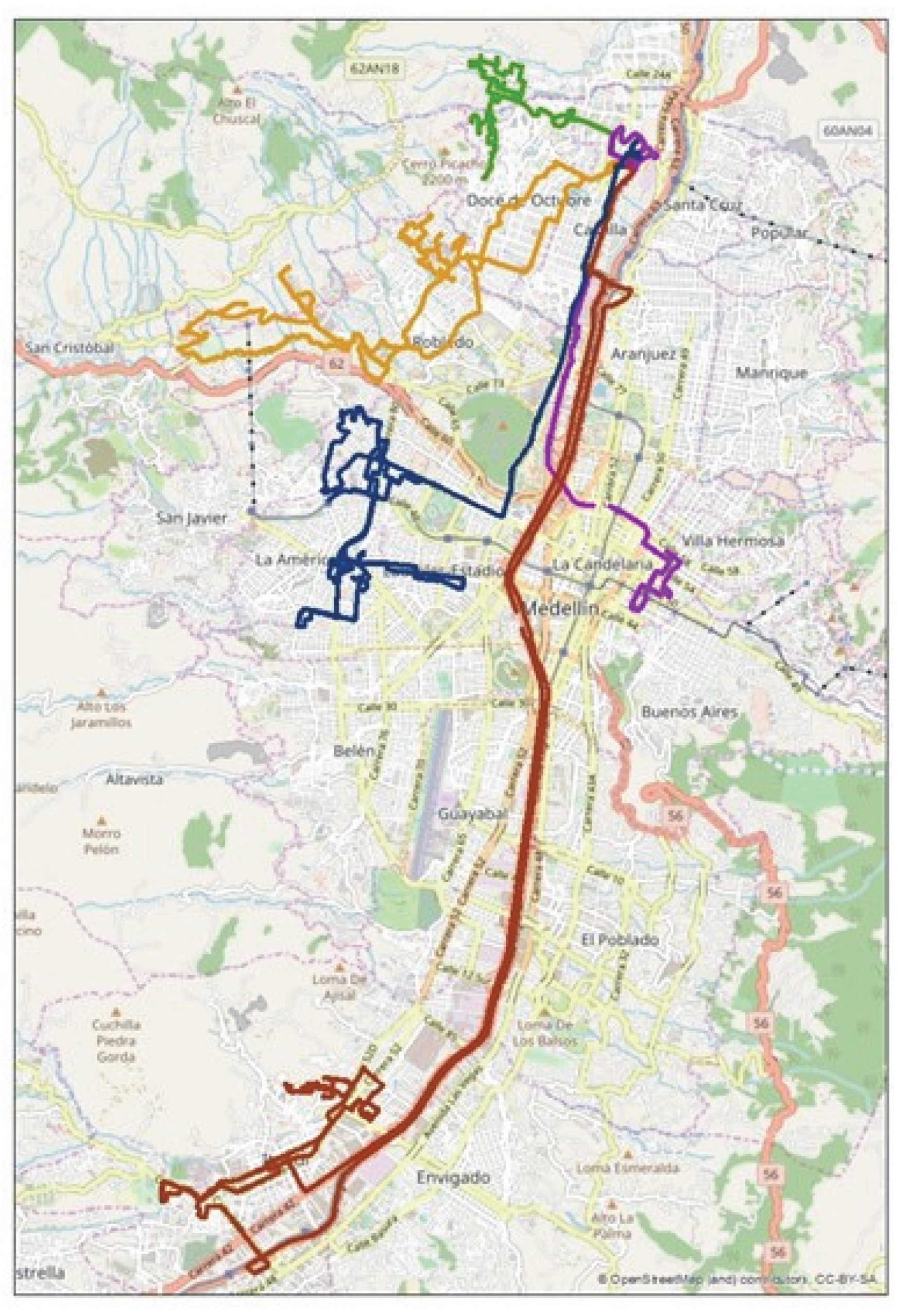
Figure 1 depicts the routes made within the city of Medellín, where each color represents a route that is created with the GPS information that reports the position of the vehicle second by second. Part of the routes is made on the main road of the urban area (the north highway, Regional Avenue, and Guayabal Avenue). These roads have an average slope of 2%; they are paved roads and, in general, dual carriageways with two lanes in each direction. The average speed is 60 km/h. Additionally, a tour was performed in the downtown area of Medellín and the western part of the city, including neighborhoods such as Laureles, Castilla, Robledo, Floresta, and Itagüí. The roads in these neighborhoods have steeper slopes than the roads described above. The average slope goes between 8% and 12%; they are dual carriageways with one lane in each direction, where the average speed is 40 km/h.
3.1. Results by Route
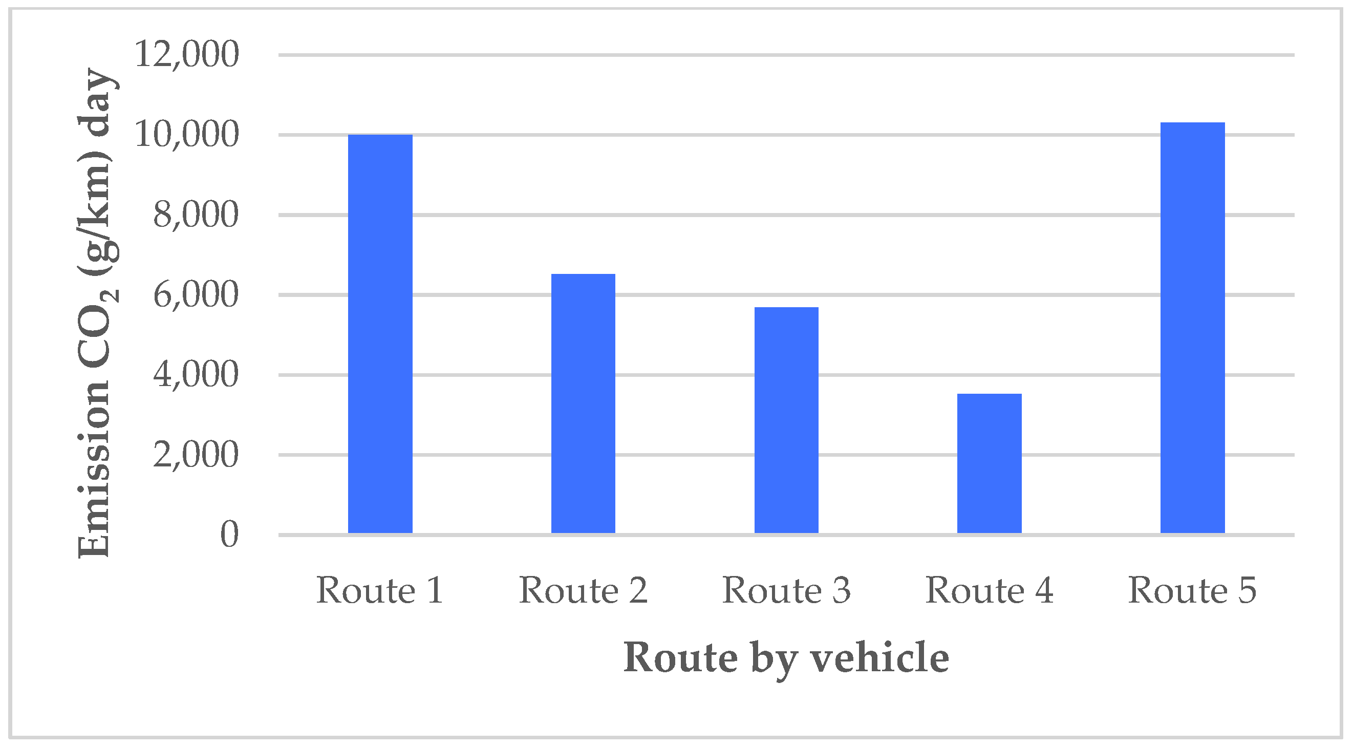
The results of the emissions from the vehicular sources of the different routes using the HBEFA model are shown in Figure 2, which represents the daily emission generated by the truck analyzed on each route. It can be observed that Route 5 is the route that emits the most CO2, with a value of 10,499.64 g/km, followed by Route 1, with 9919.82 g/km.
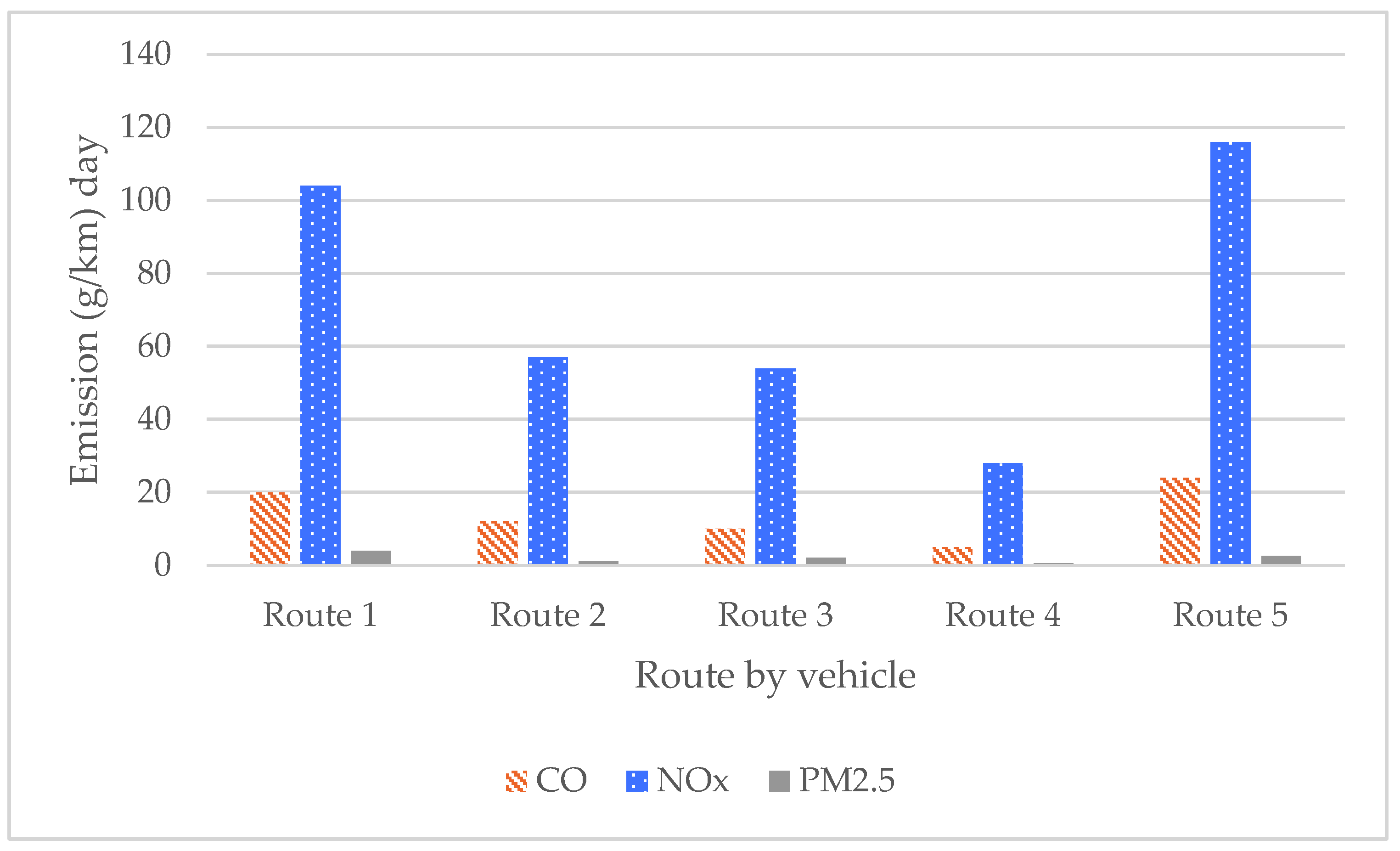
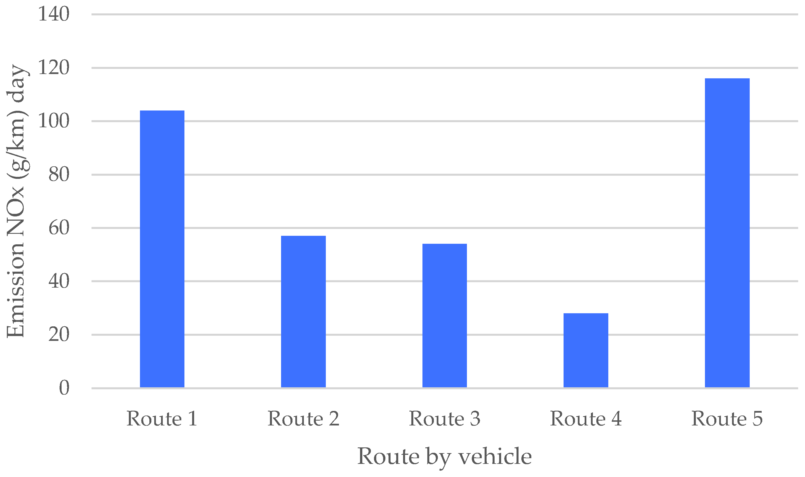
Figure 3 shows the information on the pollutants CO, NOx, and PM2.5 in g/km. It can be deduced that for all pollutants, Route 1 and Route 5 are the ones that generated the most emissions. The emission of NOX is shown in Figure 4, which indicates that Route 1 and Route 5 were the ones that emitted the most of this pollutant.
3.2. Speed
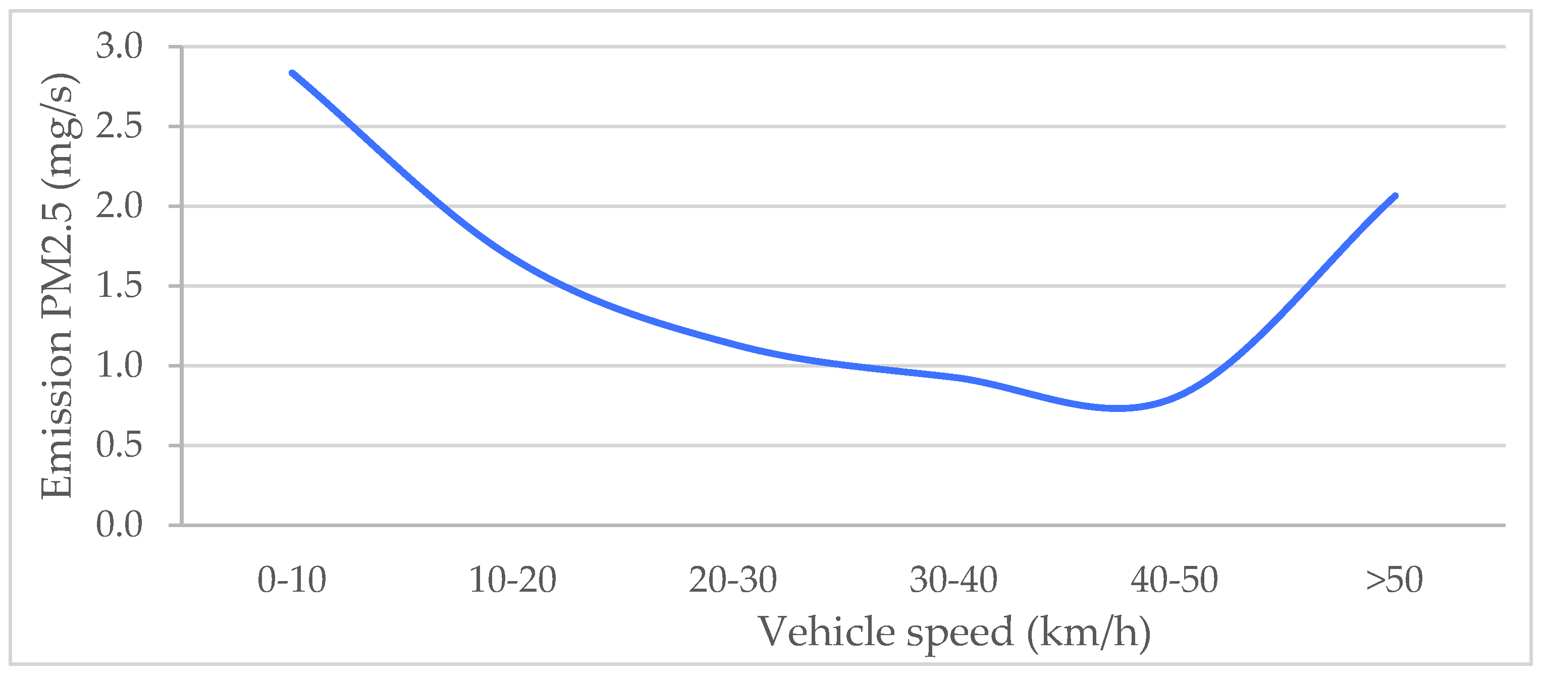
Figure 5 shows the behavior of speed and emissions. This graph was generated based on the information collected by GPS (the five analyzed routes), whereby the behavior of emissions and speed is consistent with that exposed by authors like [35,37,38]. Speeds lower than 10 km/h and greater than 50 km/h generate an increase in emissions. Based on the results, the authors recommend that trucks should move at an average speed of 50 km/h to reduce pollutant emissions in Medellín Metropolitan Area. The model estimates the emission in m/s, but the conversion is made in Figure 5 and Figure 6 for ease of analysis since it is more understandable to work in units of km/h.
3.3. Speed Comparison in HCON and HNC
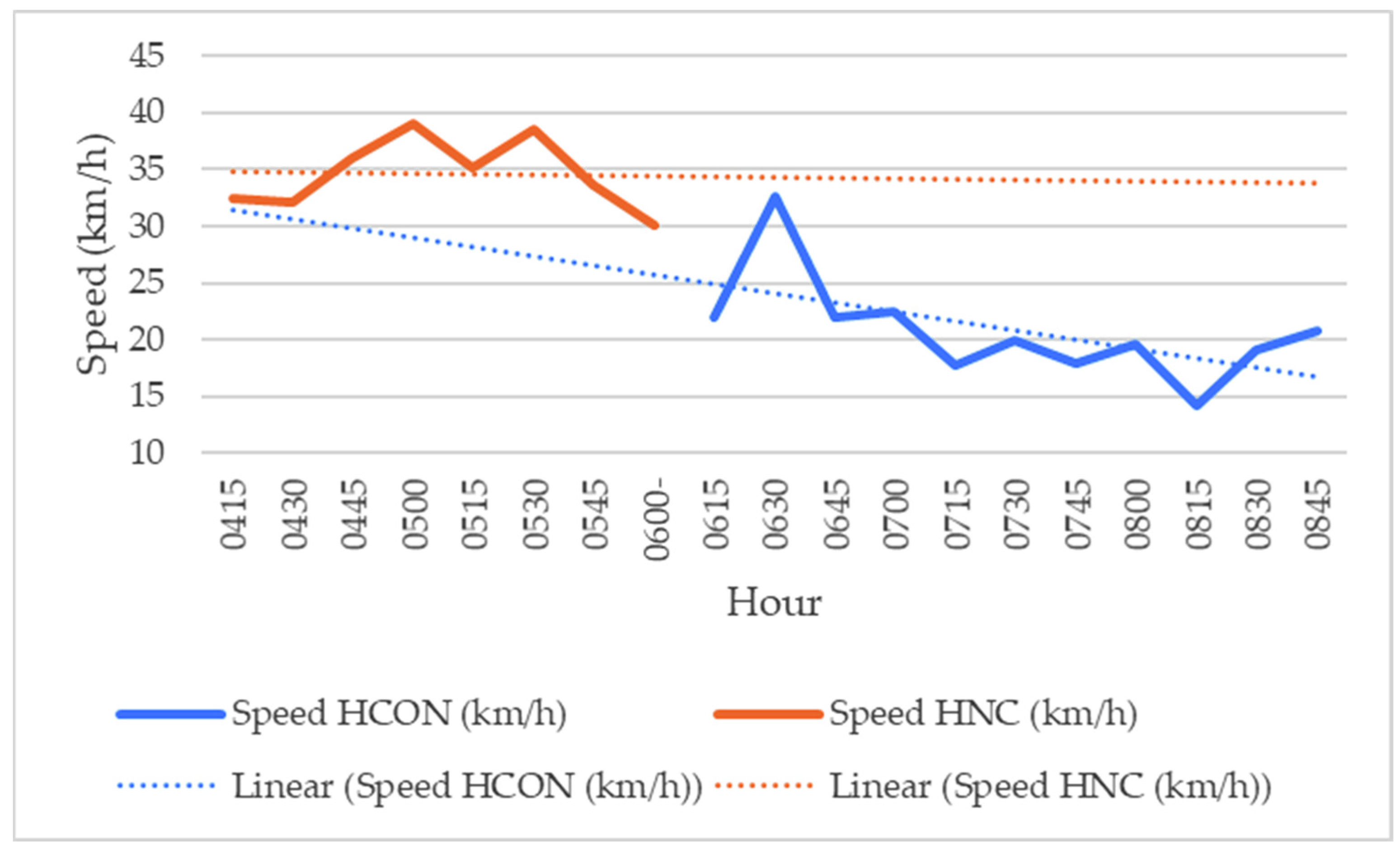
According to the available information from the five routes, a comparison was made between the speed in HCON and HNC, it is observed (see Figure 6) that between 04:10 am and 06:00 (HNC), the speed is higher, and the trend line remains the same in time. Between 06:00 and 08:45 (HCON), the speed tends to decrease as well as the trend line; in HNC, the speed remains constant; in HCON, on the contrary, it is observed that the speed changes abruptly, this is because at 06:00 it begins increased traffic flow in the city due to start working hours.
3.4. Schedule Change
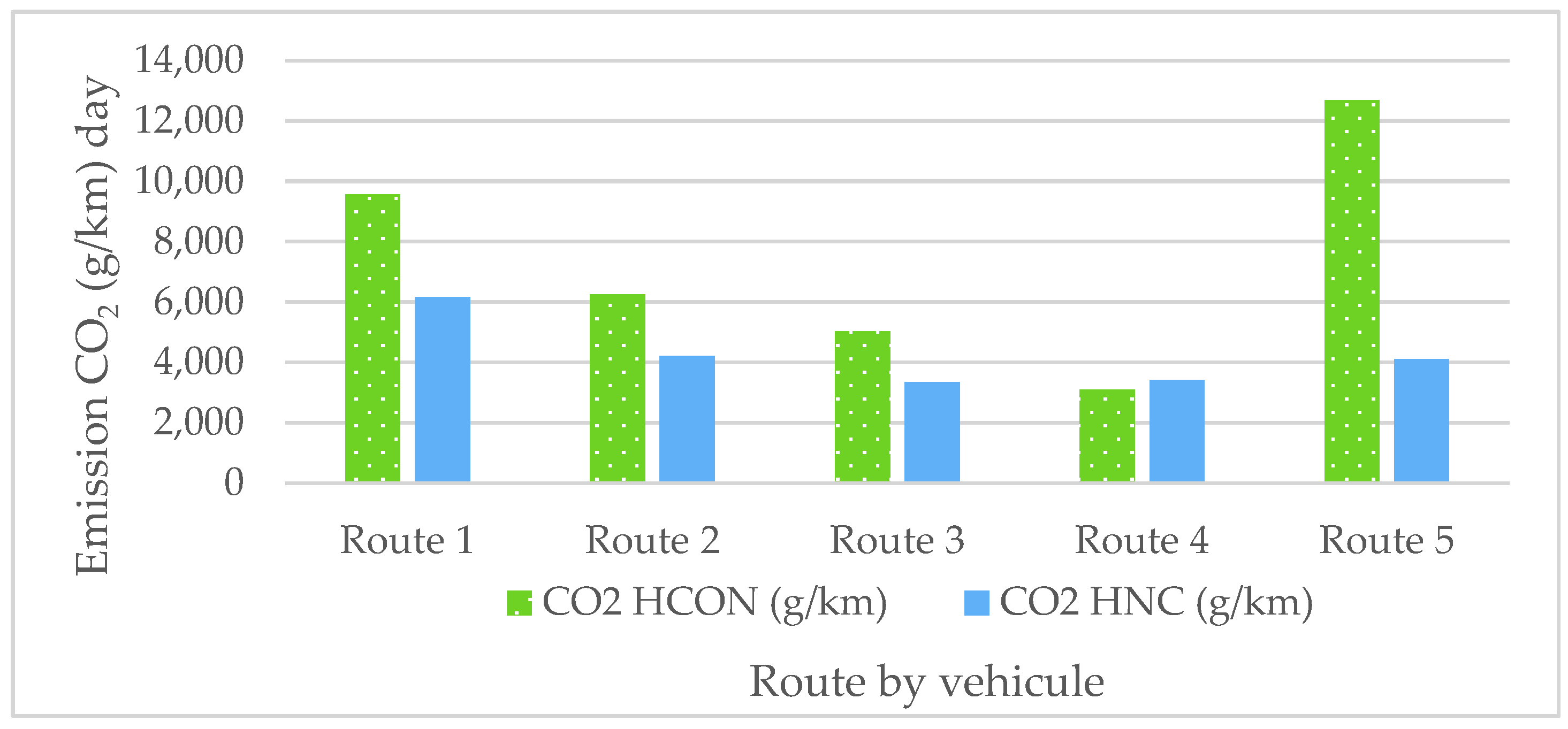
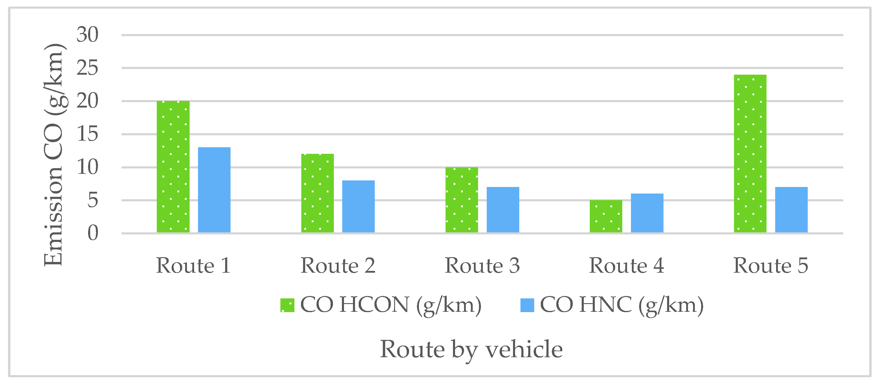
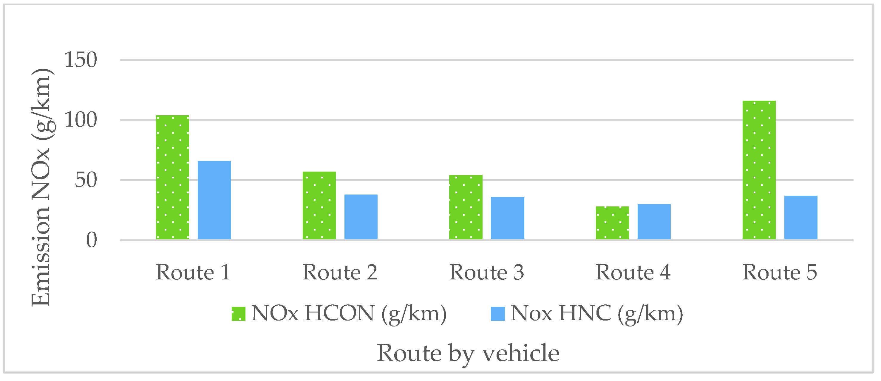
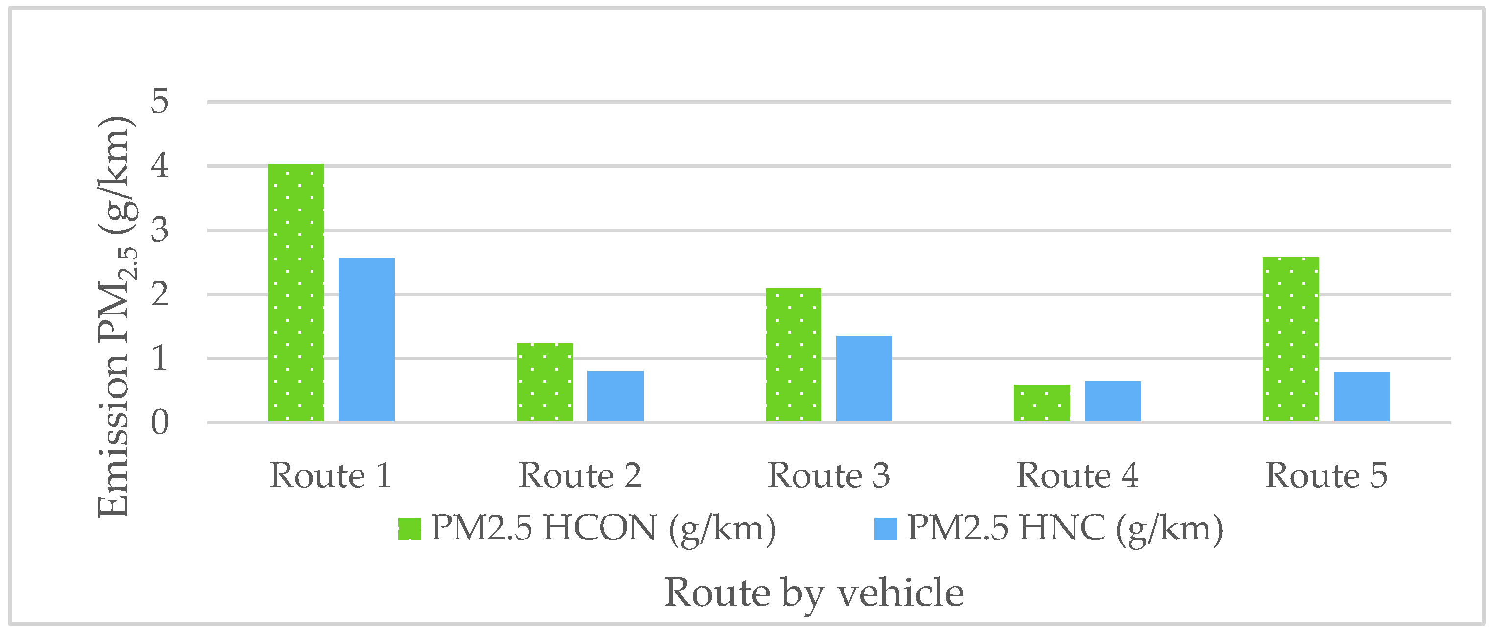
Based on the results shown above, some tours are carried out in HCON and HNC to know the behavior of emissions at different times. Figure 7, Figure 8, Figure 9 and Figure 10 show the emissions information of the CO2, CO, NOX, and PM2.5 pollutants. The results show that in all cases the emissions are lower in HNC and higher in HCON. Averagely, CO2 emissions decreased by 37% on average. Thus, for the CO and NOX, they decreased by 40% and 41% for PM2.5. The decrease in pollutants at the time change was greater than 30% in all cases.
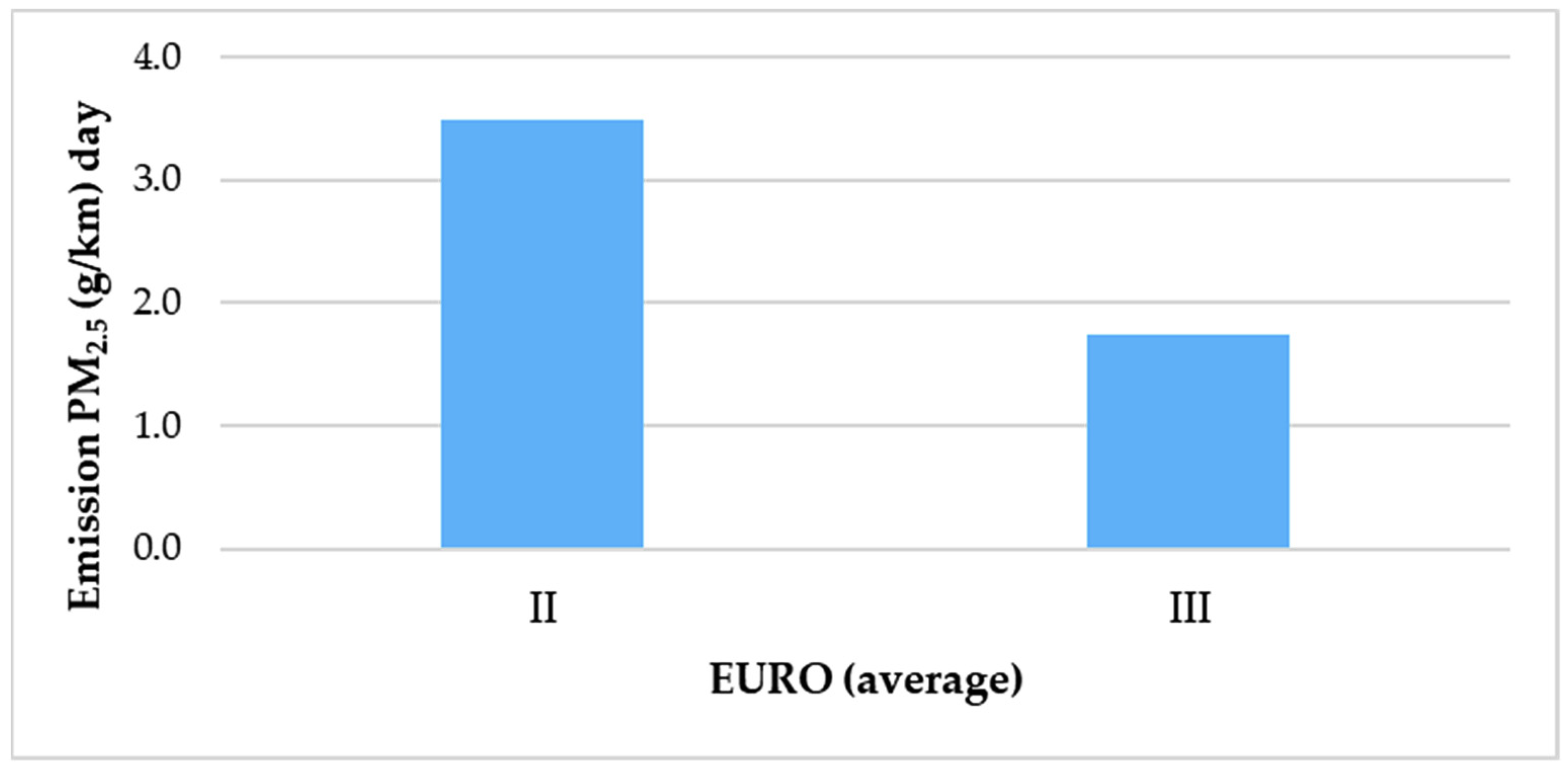
Figure 11 shows the emission information of PM2.5 according to Euro engines technology. It is shown that vehicles with Euro II emit 45% more than Euro III vehicles. These results are consistent and imply that the newer the vehicle technology, the lower the PM2.5 emission.
3.5. Comparison between Pollutant Emission Methodologies
Based on the emission results obtained through the HBEFA model, this is compared with the emission factors estimated by the University of Antioquia (UA). This University, through the GIMEL research group, has made progress since 2017 in determining the driving cycle and the real emission factors for light and heavy vehicles, considering the particularities of the technologies of the most representative vehicle fleet in the Medellín Metropolitan Area and Antioquia, their topographic and demographic conditions, and driving guidelines (calm and aggressive).
The FE emission factors (mass of a determined pollutant per unit of distance traveled) are usually determined from widely accepted models in the international arena, such as those proposed by the IVE (International Vehicle Emissions) and by the European Environment Agency (AEM) called the COPERT model. The values of each emission factor of these models are conditioned by a significant number of correction parameters that attempt to capture the reality of each country or region. However, it is advisable to measure them locally to have more approximate values of the inventories of issuers. To compare both methodologies and validate the information used in the present study, the total length of each route and emission factors (CO2 724,90 g/km and PM2.5 0,26 g/km) are required [39].
Table 5 shows the comparison between the methodology with emission factors (UA) and HBEFA. The results show that the difference between both methods is less than 20% in all studied routes. This validates that the obtained results with the HBEFA model have a good fit with the local conditions of Medellín.
Table 6 presents the model validation for both CO2 and PM2.5 using ANOVA testing hypothesis
The objective of ANOVA is to see if the initial hypothesis is fulfilled. If the value F is greater than the critical value of F, we will reject the hypothesis that the means of the groups are equal.
Analyzing the ANOVA table for CO2, the value of F is 0.06, and the critical value for F is 5.52. As F is lower, this means that the initial hypothesis is accepted in that the averages of the tests are statistically the same.
The same happens with PM2.5 as F corresponds to a value of 0.000095, and the critical value for F is 5.32.
3.6. Pollutants Amount and Health Issues
As mentioned, all these pollutants affect the environment, especially human health, contributing, for example, to respiratory diseases such as Acute Respiratory Infections (ARI) due to PM2.5 emissions. Based on the information provided by the secretary of public health of Medellín, the authors consulted information related to the health conditions of the inhabitants of different zones of the city, especially ARI, and the authors sought a relationship between ARI cases and vehicle emissions in these zones. To this effect, the authors estimated a linear model using ordinary least squares where a linear correlation analysis is performed in which the cases of ARI are compared for different zones in Medellín with the emission of PM2.5, as shown in Figure 12. The results show that an increase of 1 μg/m3 of PM2.5 can generate around 2.35 cases of ARI per year. This is an important output of the study and should be considered by the local authorities to work on public health policies to reduce the negative impact of emissions of trucks on human health.
4. Conclusions
This paper analyzes the amount of truck emissions and their variations according to changes in travel schedules or routes and the impact on human health represented by cases of Acute Respiratory Infections (ARI) due to PM2.5 emissions in Medellín, Colombia. To accomplish this, the authors collected data on commercial vehicles, including model, year, type of fuel used, Euro, and engine power trucks. The commercial vehicles were equipped with GPS to obtain second-to-second speed, location, acceleration, and deceleration, among others. All this information was used to estimate emissions with the Handbook Emission Factors for Road Transport (HBEFA) model, which provides emission factors for all current vehicle categories (passenger cars, LDV, HGV, urban buses, cars, and motorcycles).
The application of computational models is the starting point for establishing critical space-time scenarios in certain regions. The methods and model used in this study turn out to be acceptably adequate for the evaluation of traffic emissions. In this way, they could be simply applied in other cases and could be a tool for planning and evaluating the effects of traffic, as well as for measuring sensitivity to structural changes in transport.
In urban areas, speeds lower than 10 km/h and greater than 50 km/h generate an increase in emissions. The results of the investigation show that the optimal speed for truck circulation is between 40 km/h and 50 km/h. Moreover, the results show that if the vehicles circulate at that speed range, the emissions would be lower. Thus, in cities with reduced mobility due to congestion, it is recommended to change the traffic conditions for trucks through freight initiatives such as exclusive truck lanes.
In terms of human health, the results show that the increment of 1 μg/m3 in PM2.5 increases the cases of ARI by 2.35 per year. This has social and economic consequences that should be considered by the local government to improve public health in the city.
Emissions in HNC were lower than in HCON; on average, CO2 emissions were 37% lower, 40% lower for CO, 40% for NOX, and 41% for PM2.5. Thus, it is desirable that some cargo transport operations are carried out at off hours (HNC), such as during the night.
Finally, it is recommended to update the truck vehicle fleet with better EURO technology to reduce emissions. The newer the EURO technology, the lower the emissions.
Author Contributions
J.J.P.-H.: conceptualization, methodology, formal analysis, investigation, resources, writing—review and editing, visualization, supervision, project administration, funding acquisition; H.M.R.-P.: conceptualization, methodology, validation, formal analysis, resources, data curation, writing—original draft, visualization, funding acquisition; C.A.G.-C.: methodology, formal analysis, writing—review and editing, visualization, supervision, funding acquisition. All authors have read and agreed to the published version of the manuscript.
Funding
This research received no external funding.
Institutional Review Board Statement
Not applicable
Informed Consent Statement
Not applicable.
Data Availability Statement
Not applicable.
Acknowledgments
The authors acknowledge the Facultad de Minas in the Universidad Nacional de Colombia at Medellín, where the authors made their graduate and postgraduate studies.
Conflicts of Interest
The authors declare no conflict of interest.
Appendix A
Coefficients HBEFA model
- -
- Units: [mg/s]
- -
- HBEFA Model version 3
// HDV
{2.657e+04, 7076, 0.0, 1753, 0.0, 0.0}, // CO2 (total)
{54.72, 7.864, 0.0, 1.669, 0.0, 0.0}, // CO
{0.0, 0.0, 0.0, 0.0, 0.0, 0.0}, // HC
{8358, 2226, 0.0, 551.4, 0.0, 0.0}, // mKr
{305.6, 55.28, 0.0, 9.505, 0.0, 0.0}, // NOx
{7.952, 0.854, 0.0, 0.1195, 0.0, 0.0}, // PM2.5
},
{
// HDV_D_EU0
{3.251e+04, 7256, 0.0, 1631, 0.0, 0.0}, // CO2 (total)
{52.89, 12.75, 0.0, 4.547, 0.0, 0.0}, // CO
{27.82, 1.453, 0.0, 0.2468, 0.0, 0.0}, // HC
{1.023e+04, 2283, 0.0, 513.1, 0.0, 0.0 }, // mKr
{428.6, 104.2, 0.0, 24.18, 0.0, 0.0}, // NOx
{14.15, 2.335, 0.0, 0.6566, 0.0, 0.0}, // PM2.5
},
{
// HDV_D_EU1
{2.749e+04, 6533, 0.0, 1538, 0.0, 0.0}, // CO2 (total)
{58.3, 8.423, 0.0, 1.86, 0.0, 0.0}, // CO
{19.78, 1.929, 0.0, 0.2819, 0.0, 0.0}, // HC
{8647, 2055, 0.0, 483.7, 0.0, 0.0}, // mKr
{299.3, 67.56, 0.0, 14.89, 0.0, 0.0}, // NOx
{11.9, 1.744, 0.0, 0.3954, 0.0, 0.0}, // PM2.5
},
{
// HDV_D_EU2
{2.537e+04, 6723, 0.0, 1689, 0.0, 0.0}, // CO2 (total)
{41.4, 5.325, 0.0, 1.366, 0.0, 0.0}, // CO
{13.69, 1.19, 0.0, 0.1655, 0.0, 0.0}, // HC
{7980, 2115, 0.0, 531.2, 0.0, 0.0}, // mKr
{298.4, 67.21, 0.0, 15.36, 0.0, 0.0}, // NOx
{4.584, 0.789, 0.0, 0.2434, 0.0, 0.0}, // PM2.5
},
{
// HDV_D_EU3
{2.598e+04, 6712, 0.0, 1728, 0.0, 0.0}, // CO2 (total)
{51.47, 4.238, 0.0, 1.078, 0.0, 0.0}, // CO
{12.25, 0.9033, 0.0, 0.1305, 0.0, 0.0}, // HC
{8174, 2111, 0.0, 543.5, 0.0, 0.0}, // mKr
{241.1, 51.57, 0.0, 11.42, 0.0, 0.0}, // NOx
{5.436, 0.5336, 0.0, 0.1604, 0.0, 0.0}, // PM2.5
},
{
// HDV_D_EU4
{2.429e+04, 7180, 0.0, 1835, 0.0, 0.0}, // CO2 (total)
{50.68, 6.655, 0.0, 0.8349, 0.0, 0.0}, // CO
{1.119, 0.1747, 0.0, 0.03217, 0.0, 0.0}, // HC
{7639, 2259, 0.0, 577.1, 0.0, 0.0}, // mKr
{202.2, 42.34, 0.0, 8.858, 0.0, 0.0}, // NOx
{1.267, 0.131, 0.0, -0.006405, 0.0, 0.0}, // PM2.5
},
{
// HDV_D_EU5
{2.396e+04, 7231, 0.0, 1868, 0.0, 0.0}, // CO2 (total)
{51.51, 6.785, 0.0, 0.8496, 0.0, 0.0}, // CO
{1.124, 0.175, 0.0, 0.03241, 0.0, 0.0}, // HC
{7536, 2274, 0.0, 587.6, 0.0, 0.0}, // mKr
{164.8, 33.84, 0.0, 7.036, 0.0, 0.0}, // NOx
{1.305, 0.1324, 0.0, -0.007715, 0.0, 0.0}, // PM2.5
},
{
// HDV_D_EU6
{2.353e+04, 7227, 0.0, 1889, 0.0, 0.0}, // CO2 (total)
{30.78, 4.512, 0.0, 0.6383, 0.0, 0.0}, // CO
{0.7469, 0.136, 0.0, 0.03002, 0.0, 0.0}, // HC
{7400, 2273, 0.0, 594.2, 0.0, 0.0}, // mKr
{47.47, 11.68, 0.0, 2.737, 0.0, 0.0}, // NOx
{0.1279, 0.01668, 0.0, 0.00329, 0.0, 0.0}, // PM2.5
},
References
- Vieira, S.E.; Stein, R.T.; Ferraro, A.A.; Pastro, L.D.; Pedro, S.S.C.; Lemos, M.; da Silva, E.R.; Sly, P.D.; Saldiva, P.H. Urban Air Pollutants Are Significant Risk Factors for Asthma and Pneumonia in Children: The Influence of Location on the Measurement of Pollutants. Arch. Bronconeumol. 2012, 48, 389–395. [Google Scholar] [CrossRef]
- D’amato, G.; Cecchi, L.; Amato, D’.; Liccardi, G. Urban Air Pollution and Climate Change as Environmental Risk Factors of Respiratory Allergy: An Update. J. Investig. Allergol. Clin. Immunol. 2010, 20, 95–102. [Google Scholar] [PubMed]
- Rahman Khan, A.S.; Clark, N.N.; Thompson, G.J.; Wayne, W.S.; Gautam, M.; Lyons, D.W.; Hawelti, D. Idle Emissions from Heavy-Duty Diesel Vehicles: Review and Recent Data. J. Air Waste Manag. Assoc. 2006, 56, 1404–1419. [Google Scholar] [CrossRef] [PubMed] [Green Version]
- Gallardo, L.; Escribano, J.; Dawidowski, L.; Rojas, N.; de Fátima Andrade, M.; Osses, M. Evaluation of Vehicle Emission Inventories for Carbon Monoxide and Nitrogen Oxides for Bogotá, Buenos Aires, Santiago, and São Paulo. Atmos. Environ. 2012, 47, 12–19. [Google Scholar] [CrossRef]
- Sivalingam, M.; Mahapatra, S.S.; Hansdah, D.; Horák, B. Validation of Some Engine Combustion and Emission Parameters of a Bioethanol Fuelled Di Diesel Engine Using Theoretical Modelling. Alexandria Eng. J. 2015, 54, 993–1002. [Google Scholar] [CrossRef] [Green Version]
- Hong, J.; Goodchild, A. Land Use Policies and Transport Emissions: Modeling the Impact of Trip Speed, Vehicle Characteristics and Residential Location. Transp. Res. Part D Transp. Environ. 2014, 26, 47–51. [Google Scholar] [CrossRef]
- Propper, R.; Wong, P.; Bui, S.; Austin, J.; Vance, W.; Alvarado, Á.; Croes, B.; Luo, D. Ambient and Emission Trends of Toxic Air Contaminants in California. Environ. Sci. Technol. 2015, 49, 11329–11339. [Google Scholar] [CrossRef] [PubMed] [Green Version]
- Wu, B.; Shen, X.; Cao, X.; Zhang, W.; Wu, H.; Yao, Z. Carbonaceous Composition of PM2.5 Emitted from on-Road China III Diesel Trucks in Beijing, China. Atmos. Environ. 2015, 116, 216–224. [Google Scholar] [CrossRef]
- Sociedad Nacional de Mineria, Petroleo y Energía. El Gas Natural Vehícular-GNV; Sociedad Nacional de Minería, Petróleo y Energía: Magdalena del Mar Lima, Peru, 2011. [Google Scholar]
- U.S. Environmental Protection Agency; Office of Research and Development; National Center for Environmental Assessment. U.S. EPA. Health Assessment Document For Diesel Engine Exhaust (Final 2002); Environmental Protection Agency: Washington, DC, USA, 2002.
- Pino-Cortés, E.; Díaz-Robles, L.A.; Cubillos, F.; Fu, J.S.; Vergara-Fernández, A. Sensitivity Analysis of Biodiesel Blends on Benzo[a]Pyrene and Main Emissions Using MOVES: A Case Study in Temuco, Chile. Sci. Total Environ. 2015, 537, 352–359. [Google Scholar] [CrossRef] [PubMed]
- European Parliament and Council. REGULATION (EU) 2019/1242 OF THE EUROPEAN PARLIAMENT AND OF THE COUNCIL of 20 June 2019 Setting CO2 Emission Performance Standards for New Heavy-Duty Vehicles and Amending Regulations (EC) No 595/2009 and (EU) 2018/956 of the European Parliament and of Th; European Union: Paris, France, 2019; Volume 198. [Google Scholar]
- Rexeis, M.; Hausberger, S.; Kühlwein, J.; Luz, R. Update of Emission Factors for EURO 5 and EURO 6 Vehicles for the HBEFA Version 3.2; Graz University of Technology: Graz, Austria, 2013; Volume 43. [Google Scholar]
- Yusuf, A.A.; Inambao, F.L.; Ampah, J.D. Evaluation of Biodiesel on Speciated PM2.5, Organic Compound, Ultrafine Particle and Gaseous Emissions from a Low-Speed EPA Tier II Marine Diesel Engine Coupled with DPF, DEP and SCR Filter at Various Loads. Energy 2022, 239, 121837. [Google Scholar] [CrossRef]
- Yusuf, A.A.; Dankwa Ampah, J.; Soudagar, M.E.M.; Veza, I.; Kingsley, U.; Afrane, S.; Jin, C.; Liu, H.; Elfasakhany, A.; Buyondo, K.A. Effects of Hybrid Nanoparticle Additives in N-Butanol/Waste Plastic Oil/Diesel Blends on Combustion, Particulate and Gaseous Emissions from Diesel Engine Evaluated with Entropy-Weighted PROMETHEE II and TOPSIS: Environmental and Health Risks of Plastic Waste. Energy Convers. Manag. 2022, 264, 115758. [Google Scholar] [CrossRef]
- Boldo, E.; Querol, X. Nuevas Políticas Europeas de Control de La Calidad Del Aire: ¿un Paso Adelante Para La Mejora de La Salud Pública? New European Policies for Air Pollution Control: A Step Forward in Improving Public Health? Gac Sanit 2014, 28, 263–266. [Google Scholar] [CrossRef] [PubMed]
- Aguiar Gil, D.; Calle Palacio, J.M.; Hernández Vasco, D.F.; González Manosalva, J.L. Medellín y Su Calidad Del Aire; Instituto Tecnológico Metropolitano: Medellín, Colombia, 2016. [Google Scholar]
- Zhang, Y.; Yao, Z.; Shen, X.; Liu, H.; He, K. Chemical Characterization of PM2.5 Emitted from on-Road Heavy-Duty Diesel Trucks in China. Atmos. Environ. 2015, 122, 885–891. [Google Scholar] [CrossRef]
- Arango, J.H. Calidad de Los Combustibles en Colombia. Rev. Ing. Univ. los Andes 2009, 29, 100–108. [Google Scholar] [CrossRef]
- Clean Air Institute; Área metropolitana Valle de Aburrá. Estrategia Ambiental Integrada Para una Movilidad Sustentable en el Área Metropolitana del Valle de Aburrá; Área Metropolitana del Valle de Aburrá: Medellín, Colombia, 2011. [Google Scholar]
- ESCAP-Economic and Social Commission for Asia and the Pacific; United Nations. Transport and Communications Bulletin for Asia and the Pacific No. 80 Sustainable Urban Freight Transport; United Nations: Bangkok, Thailand, 2011. [Google Scholar]
- Ministerio de ambiente y Desarrollo Sostenible, República de Colombia. Resolución 2254. “Por la Cual se Adopta la Norma de Calidad del Aire Ambiente y se Dictan Otras Disposiciones”; Ministerio de Ambiente y Desarrollo Sostenible: Medellín, Colombia, 2017; pp. 1–11.
- Ballester, F.; Llop, S.; Querol, X.; Esplugues, A. Evolución de Los Riesgos Ambientales en el Contexto de la Crisis Económica. Informe SESPAS 2014. Gac. Sanit. 2014, 28, 51–57. [Google Scholar] [CrossRef] [PubMed] [Green Version]
- Área Metropolitana del Valle de Aburrá; Universidad Pontificia Bolivariana. Inventario de Emisiones Atmosféricas del Valle de Aburrá, Año Base 2013; Área Metropolitana del Valle de Aburrá: Medellín, Colombia, 2014. [Google Scholar]
- Morales-Pinzón, T.; Arias Mendoza, J.J. Contaminación Vehicular En La Conurbación Pereira-Dosquebradas. Luna Azul 2013, 37, 101–129. [Google Scholar]
- Janssen, N.A.H.; Brunekreef, B.; van Vliet, P.; Aarts, F.; Maliefste, K.; Harssema, H.; Fischer, P. The Relationship between Air Pollution from Heavy Traffic and Allergic Sensitization, Bronchial Byperresponsiveness, and Respiratory Symptoms in Dutch Schoolchildren. Environ. Health Perspect. 2003, 111, 1512–1518. [Google Scholar] [CrossRef] [PubMed] [Green Version]
- Pérez, L.; Sunyer, J.; Künzli, N. Estimating the Health and Economic Benefits Associated with Reducing Air Pollution in the Barcelona Metropolitan Area (Spain). Gac. Sanit. 2009, 23, 287–294. [Google Scholar] [CrossRef] [PubMed] [Green Version]
- Wallace, H.W.; Jobson, B.T.; Erickson, M.H.; McCoskey, J.K.; VanReken, T.M.; Lamb, B.K.; Vaughan, J.K.; Hardy, R.J.; Cole, J.L.; Strachan, S.M.; et al. Comparison of Wintertime CO to NO x Ratios to MOVES and MOBILE6.2 on-Road Emissions Inventories. Atmos. Environ. 2012, 63, 289–297. [Google Scholar] [CrossRef]
- Gonzalez Valencia, A.; Gomez Gallo, M.H. Diagnóstico Ambiental y Técnico Mecánico del Sector Volquetas del Área Metropolitana del Valle de Aburrá. Prod. + Limpia 2010, 5, 39–57. [Google Scholar]
- Borrego, C.; Amorim, J.H.; Tchepel, O.; Dias, D.; Rafael, S.; Sá, E.; Pimentel, C.; Fontes, T.; Fernandes, P.; Pereira, S.R.; et al. Urban Scale Air Quality Modelling Using Detailed Traffic Emissions Estimates. Atmos. Environ. 2016, 131, 341–351. [Google Scholar] [CrossRef] [Green Version]
- Gallus, J.; Kirchner, U.; Vogt, R.; Börensen, C.; Benter, T. On-Road Particle Number Measurements Using a Portable Emission Measurement System (PEMS). Atmos. Environ. 2016, 124, 37–45. [Google Scholar] [CrossRef]
- Keller, M.; MK Consulting. HEBFA-Status, Outlook HBEFA-Overview; Keller Consulting: Kansas City, MO, USA, 2014. [Google Scholar]
- Hausberger, S.; Rexeis, M.; Zallinger, M.; Luz, R. Emission Factors from the Model PHEM for the HBEFA Version 3; Balint, G., Antala, B., Carty, C., Mabieme, J.-M.A., Amar, I.B., Kaplanova, A., Eds.; Graz University of Technology: Graz, Austria, 2009; Volume 7. [Google Scholar]
- Maneva Mitrovikj, K.; Skácel, F.; Maneva Mitrovikj, K.; Skácel, F. Verification of Traffic Emission Factors Using Measurements in a Short Tunnel in the Czech Republic. Atmósfera 2019, 32, 213–223. [Google Scholar] [CrossRef]
- Zamboni, G.; André, M.; Roveda, A.; Capobianco, M. Experimental Evaluation of Heavy Duty Vehicle Speed Patterns in Urban and Port Areas and Estimation of Their Fuel Consumption and Exhaust Emissions. Transp. Res. Part D Transp. Environ. 2015, 35, 1–10. [Google Scholar] [CrossRef]
- Posada-Henao, J.J. Efecto de La Cantidad de Carga en el Consumo de Combustible en Camiones; Universidad Nacional de Colombia, Sede Medellín: Medellín, Colombia, 2012. [Google Scholar]
- Brodrick, C.-J.; Dwyer, H.A.; Farshchi, M.; Harris, D.B.; King, F.G. Effects of Engine Speed and Accessory Load on Idling Emissions from Heavy-Duty Diesel Truck Engines. J. Air Waste Manag. Assoc. 2002, 52, 1026–1031. [Google Scholar] [CrossRef] [PubMed]
- Goel, R.; Guttikunda, S.K.; Mohan, D.; Tiwari, G. Benchmarking Vehicle and Passenger Travel Characteristics in Delhi for On-Road Emissions Analysis. Travel Behav. Soc. 2015, 2, 88–101. [Google Scholar] [CrossRef]
- Agudelo Santamaria, J.R.; Grupo de Manejo Eficiente de la Energía (GIMEL). Articulación Universidad-Empresa-Estado Para Establecer los Factores de Emisión Reales de Vehículos Pesados en el Valle de Aburrá (FEVA-II); Universidad de Antioquia: Medellín, Colombia, 2019. [Google Scholar]
Figure 1.
Tours made with GPS: Route 1 (Blue) (La América and San Javier), Route 2 (Red) (Itagüí city), Route 3 (Purple) (Downtown), Route 4 (Orange) (October 12 and Robledo) and route 5 (Green) (Castilla).
Figure 1.
Tours made with GPS: Route 1 (Blue) (La América and San Javier), Route 2 (Red) (Itagüí city), Route 3 (Purple) (Downtown), Route 4 (Orange) (October 12 and Robledo) and route 5 (Green) (Castilla).

Figure 2.
Emission CO2 by route.

Figure 3.
Emission of CO, NOx, and PM2.5 of the different routes.

Figure 4.
NOX emissions of the different routes.

Figure 5.
PM2.5 Emission vs. Speed.

Figure 6.
Speed HCON vs. HNC.

Figure 7.
CO2 emission in HCON and HNC.

Figure 8.
CO emission in HCON and HNC.

Figure 9.
NOX emission in HCON and HNC.

Figure 10.
Emission of PM2.5 in HCON and HNC.

Figure 11.
Emission PM2.5 vs. Euro.

Figure 12.
Cases ARI vs. Emission PM2.5.


Table 1.
Air pollutants.
| Pollutant | Origin and Health Effects |
|---|---|
| CO | Product of incomplete combustion of hydrocarbons. Intoxicates the blood preventing oxygen transport. |
| NOX | Released into the air from the emission of vehicles (combustion). Irritation eyes, nose, throat, and lungs, dilatation of throat and upper respiratory tract, reducing oxygenation of body tissues. |
| SOX | Produced by gases from car leakages. Levels 1–10 ppm induces increased respiratory rate and pulse. |
| PM | The main anthropogenic sources of small particles include burning solid fuels such as wood and coal. They can be inhaled and easily penetrate the human respiratory system causing effects on people’s health. |
Table 2.
Fuel type vs. Pollutant concentration.
| Pollutant | Fuel | ||
|---|---|---|---|
| Gasoline | Diesel | NGV | |
| CO | High | Medium | Low |
| NOX | Medium | High | High |
| SOX | Medium | High | Low |
| PM2.5 | Medium | High | Low |
Table 3.
Vehicle characteristics.
| Brand | Year | Fuel Type | Euro | Cylindrical |
|---|---|---|---|---|
| Chevrolet | 2011 | Diesel | III | 2771 |
| Hino | 2015 | Diesel | III | 5123 |
| Chevrolet | 2005 | Diesel | III | 2771 |
| Chevrolet | 2013 | Diesel | III | 2771 |
| Chevrolet | 2007 | Diesel | III | 2700 |
Table 4.
Summary of route information.
| Route | Initial Hour hhmmss | Final Hour hhmmss | Time (h) | Average Speed (km/h) | Max. Speed (km/h) | Distance (Km) |
|---|---|---|---|---|---|---|
| 1 | 04:20:16 | 11:02:44 | 5 | 23.5 | 76.0 | 31.0 |
| 2 | 04:36:44 | 13:02:14 | 7 | 22.0 | 67.0 | 52.0 |
| 3 | 05:10:22 | 13:14:37 | 8 | 23.9 | 74.0 | 15.4 |
| 4 | 04:38:45 | 13:55:09 | 8 | 18.8 | 57.0 | 31.5 |
| 5 | 04:53:59 | 14:35:54 | 9 | 12.7 | 40.0 | 17.3 |
Table 5.
Summary information covered.
| Route | Emissions HBEFA | Emissions UA | Comparison (%) | |||
|---|---|---|---|---|---|---|
| CO2 | PM2.5 | CO2 | PM2.5 | CO2 | PM2.5 | |
| (g/km) | (g/km) | (g/km) | (g/km) | (g/km) | (g/km) | |
| 1 | 9566.00 | 4.04 | 11,235.95 | 4.03 | 17.5 | 0.2 |
| 2 | 6247.00 | 1.24 | 6524.10 | 1.30 | 4.4 | 4.8 |
| 3 | 5027.00 | 2.09 | 5690.47 | 2.21 | 13.2 | 5.7 |
| 4 | 3099.00 | 0.59 | 3530.26 | 0.70 | 13.9 | 18.6 |
| 5 | 12,685.00 | 2.58 | 12,540.77 | 2.34 | 1.1 | 9.3 |
Table 6.
Model validation for CO2 and PM2.5 using ANOVA testing hypothesis.
| Validation CO2 | ||||||
|---|---|---|---|---|---|---|
| Origin of Variations | Sum of Squares | Degrees of Freedom | Average of the Squares | F | Probability | Critical Value for F |
| Between groups | 839,579.60 | 1 | 839,579.60 | 0.06 | 0.82 | 5.32 |
| Within groups | 116,588,611.81 | 8 | 14,573,576.48 | |||
| Total | 117,428,191.41 | 9 | ||||
| Validation PM2.5 | ||||||
| Origin of Variations | Sum of Squares | Degrees of Freedom | Average of the Squares | F | Probability | Critical Value for F |
| Between groups | 1.60 × 10⁻⁴ | 1 | 1.60 × 10⁻⁴ | 9.55 × 10⁻⁵ | 9.92 × 10⁻¹ | 5.32 |
| Within groups | 13.4 × 101 | 8 | 1.68 | |||
| Total | 13.40696 | 9 | ||||
Publisher’s Note: MDPI stays neutral with regard to jurisdictional claims in published maps and institutional affiliations. |
© 2022 by the authors. Licensee MDPI, Basel, Switzerland. This article is an open access article distributed under the terms and conditions of the Creative Commons Attribution (CC BY) license (https://creativecommons.org/licenses/by/4.0/).
Share and Cite
MDPI and ACS Style
Posada-Henao, J.J.; Restrepo-Peña, H.M.; González-Calderón, C.A. Simulation of Air Pollutants Emission by Trucks and Their Health Effects. Atmosphere 2022, 13, 1691. https://0-doi-org.brum.beds.ac.uk/10.3390/atmos13101691
AMA Style
Posada-Henao JJ, Restrepo-Peña HM, González-Calderón CA. Simulation of Air Pollutants Emission by Trucks and Their Health Effects. Atmosphere. 2022; 13(10):1691. https://0-doi-org.brum.beds.ac.uk/10.3390/atmos13101691
Chicago/Turabian StylePosada-Henao, John Jairo, Heliana Marcela Restrepo-Peña, and Carlos A. González-Calderón. 2022. "Simulation of Air Pollutants Emission by Trucks and Their Health Effects" Atmosphere 13, no. 10: 1691. https://0-doi-org.brum.beds.ac.uk/10.3390/atmos13101691
Note that from the first issue of 2016, this journal uses article numbers instead of page numbers. See further details here.