Article

Variability of the Aerosol Content in the Tropical Lower Stratosphere from 2013 to 2019: Evidence of Volcanic Eruption Impacts

by
Mariam Tidiga
1,
Gwenaël Berthet
1,*,
Fabrice Jégou
1,
Corinna Kloss
1,
Nelson Bègue
2,
Jean-Paul Vernier
3,4,
Jean-Baptiste Renard
1,
Adriana Bossolasco
1,5,
Lieven Clarisse
6,
Ghassan Taha
7,8,
Thierry Portafaix
2,
Terry Deshler
9,
Frank G. Wienhold
10,
Sophie Godin-Beekmann
11,
Guillaume Payen
12,
Jean-Marc Metzger
12,
Valentin Duflot
2 and
Nicolas Marquestaut
12
1
Laboratoire de Physique de Chimie de l’Environnement et de l’Espace (LPC2E), CNRS, Université d’Orléans, 45071 Orléans, France
2
Laboratoire de l’Atmosphère et des Cyclones (LACy, UMR 8105 CNRS, Météo-France), Université de la Réunion, 97400 Saint-Denis de La Réunion, France
3
NASA Langley Research Center, Hampton, VA 23681, USA
4
National Institute of Aerospace (NIA), Hampton, VA 23681, USA
5
Now at Laboratorio de Física de la Atmósfera, INFINOA (CONICET), Universidad Nacional de Tucumán, San Miguel de Tucuman 40000, Argentina
6
Spectroscopy, Quantum Chemistry and Atmospheric Remote Sensing, Université Libre de Bruxelles (ULB), 1050 Bruxelles, Belgium
7
Morgan State University, Baltimore, MD 21251, USA
8
NASA Goddard Space Flight Center, Greenbelt, MD 20771, USA
9
Department of Atmospheric Science, University of Wyoming, Laramie, WY 82071, USA
10
Institute for Atmospheric and Climate Science (IAC), Federal Institute of Technology (ETHZ), 8092 Zurich, Switzerland
11
LATMOS/IPSL, UVSQ Université Paris-Saclay, Sorbonne Université, CNRS, 75000 Paris, France
12
Observatoire des Sciences de l’Univers de La Réunion (OSU-Réunion), UAR 3365, Université de la Réunion, CNRS, Météo-France, 97400 Saint-Denis de La Réunion, France
*
Author to whom correspondence should be addressed.
Submission received: 28 November 2021 / Revised: 24 January 2022 / Accepted: 26 January 2022 / Published: 31 January 2022
(This article belongs to the Special Issue Feature Papers in Atmosphere Science)

Abstract

:
This paper quantifies the tropical stratospheric aerosol content as impacted by volcanic events over the 2013–2019 period. We use global model simulations by the Whole Atmosphere Community Climate Model (WACCM) which is part of the Community Earth System Model version 1.0 (CESM1). WACCM is associated with the Community Aerosol and Radiation Model for Atmospheres (CARMA) sectional aerosol microphysics model which includes full sulphur chemical and microphysical cycles with no a priori assumption on particle size. Five main volcanic events (Kelud, Calbuco, Ambae, Raikoke and Ulawun) have been reported and are shown to have significantly influenced the stratospheric aerosol layer in the tropics, either through direct injection in this region or through transport from extra-tropical latitudes. Space-borne data as well as ground-based lidar and balloon-borne in situ observations are used to evaluate the model calculations in terms of aerosol content, vertical distribution, optical and microphysical properties, transport and residence time of the various volcanic plumes. Overall, zonal mean model results reproduce the occurrence and vertical extents of the plumes derived from satellite observations but shows some discrepancies for absolute values of extinction and of stratospheric aerosol optical depth (SAOD). Features of meridional transport of the plumes emitted from extra-tropical latitudes are captured by the model but simulated absolute values of SAOD differ from 6 to 200% among the various eruptions. Simulations tend to agree well with observed in situ vertical profiles for the Kelud and Calbuco plumes but this is likely to depend on the period for which comparison is done. Some explanations for the model–measurement discrepancies are discussed such as the inaccurate knowledge of the injection parameters and the presence of ash not accounted in the simulations.

1. Introduction

Changes in the decadal rate of global warming have been attributed to several factors including temporal changes in natural and anthropogenic emissions, solar irradiance, and the variability of the stratospheric aerosol load [1,2]. Sulphate aerosol in the stratosphere is expected to be mainly controlled by natural emissions of carbonyl sulfide (OCS) and sulphur dioxide (SO2), although anthropogenic contributions remain debated [3,4]. The subsequent formation of droplets composed of sulphuric acid and water through binary homogeneous nucleation, with an additional supply of smaller amounts of meteoritic and other non-sulphate material [5,6], is responsible for the presence of a ubiquitous stratospheric aerosol layer. The largest source of sulphate aerosols is due to explosive volcanic eruptions which inject large quantities of SO2 directly into the stratosphere. Produced volcanic plumes have the potential to impact the global radiative budget with warming in the stratosphere and cooling in the troposphere [7,8,9]. Furthermore, increased particle loads provide sites for heterogeneous chemical reactions enhancing stratospheric ozone depletion [10]. The last major eruption was Mount Pinatubo in 1991 (15.1° N, 120.3° E) which injected 14–23 Tg of SO2 into the stratosphere and subsequently produced a rapid global-averaged cooling at the Earth’s surface of several tenths of degrees over the following year [11], despite the significant warming effects of a coincident El Niño event [12].
Several studies have been focused on the general impacts of moderate-magnitude explosive volcanic eruptions. When such an event is considered individually, negligible effects on climate have been derived compared to large-magnitude eruptions [13,14]. A reduction of ~4% in the ozone burden have been reported in the mid-latitude lower stratosphere impacted by the Sarychev volcanic plume [15] but the most important impact has been inferred on stratospheric polar ozone with further loss of 25% in the Antarctic vortex resulting from the Calbuco aerosols [16].
The relatively high-frequency of moderate-magnitude eruptions is likely to modulate and maintain the global stratospheric aerosol burden significantly above background levels (i.e., conditions unperturbed by sporadic injections of aerosols or gaseous precursors by volcanoes or fires) as shown after year 2000 [17]. As a result, the cumulative impacts have been identified as a possible factor on recent climate trends [18,19] with a reported global cooling of –0.07 °C over the 2000 decade. Furthermore, the recently observed slowdown of the stratospheric circulation in the Northern Hemisphere would be by 50% attributable to stratospheric aerosol from post-2008 moderate-magnitude volcanic eruptions, reflecting that such events should no longer be neglected in climate simulations [20].
A moderate-magnitude eruption occurring at mid-latitudes typically modulates the stratospheric aerosol burden on scales of months [16,21,22]. Aerosols are redistributed horizontally after the eruption before being homogenized at the hemispheric scale. They descend diabatically to the mid-latitude lowermost stratosphere where they can be eventually removed in the troposphere through quasi-isentropic transport in tropopause folds [23]. The horizontal extent of mid-latitude volcanic plumes has been shown to be clearly bounded by the fluctuations of dynamical subtropical barrier and the polar vortex [24,25]. Volcanic aerosols produced from events which take place at tropical latitudes are rapidly transported zonally, especially if the volcanic plume is injected just below the tropical reservoir, with the mean stratospheric winds. They propagate upward via the ascending branch of the Brewer-Dobson circulation (BDC) within the tropical reservoir with reduced exchange with the extratropics [26], thus prolonging the particle residence time in the stratosphere [4,17]. This dynamical feature is mainly expected for eruptions injecting material above the tropical tropopause layer (TTL). The quasi-biennial oscillation (QBO) also influences the poleward transport of gas precursors and aerosols which become more effective during the QBO westerly phase [27,28]. Meridional transport and mixing between the tropics and extratropics are more efficient within the TTL which favors the fast horizontal propagation of volcanic plumes produced in the lowermost stratosphere [29]. Volcanic plume dynamics can be useful to derive vertical motion rates associated with the BDC from observations [30,31,32].
Microphysical processes through growth, coagulation, evaporation and sedimentation take place simultaneously as the volcanic particles are transported. Comprehensive simulations of volcanic plume properties and propagation patterns using global Climate-Chemistry models accounting for dynamical, chemical and microphysical mechanisms are a prerequisite of proper quantification of the impacts of volcanic aerosols on stratospheric ozone chemistry and radiative forcing. In turn, a robust simulation of a volcanic plume space-time extent is expected to critically depend on the knowledge of the injection parameters, in particular the amount of sulphur, the plume altitude and the injection timing. This can be achieved through comparisons with observations. As an example, a global simulation of the mid-latitude past moderate eruption of the Sarychev volcano in June 2009 has been assessed using satellite and balloon-borne in situ observations [22]. Even with a simple injection sequence, this study has demonstrated the ability of the model to reproduce both local and hemispherical features of this specific volcanic plume. Since then, several eruptions have impacted the stratospheric aerosol budget and for some of them it is not clear whether they can be simulated with the same efficiency as for the Sarychev event in terms of content and evolution of SO2 and sulphuric acid particles.
Our study investigates the robustness of a global model in its ability to simulate the optical and transport patterns of an ensemble of eruptions considering the full 2013–2019 period. Five main events have occurred over this period: Kelud in 2014, Calbuco in 2015, Ambae in 2018, Raikoke in 2019 and Ulawun in 2019. We use global model simulations using the global Community Earth System Model version 1.0 (CESM1) with its Whole Atmosphere Community Climate Model (WACCM) module for the simulation of the atmosphere, along with the sectional Community Aerosol and Radiation Model for Atmospheres module (CARMA) explicitly computing aerosol microphysical processes to derive the physical properties of the plumes and their time-space extent.
We specifically examine how these eruptions have influenced the stratospheric aerosol content on tropical latitudes, either for sulphur injection at mid-latitude or directly in the tropics, and compare the simulations with satellite data at a large scale to evaluate the simulated plume evolution and aerosol residence times. This work particularly benefits from ground-based and in situ observations, rarely available in tropical regions, and not used for comparisons with model outputs so far. This provides a model assessment at a more local scale.
The model initialisation is driven from information about injection parameters available in the literature. We use updated and improved satellite SO2 datasets in comparison with former studies to examine the modelled evolution of SO2. We discuss explanations for the model–measurement discrepancies at the large and local scale, such as the pertinence of the injection parameters and the importance of ash co-injection as reported in recent studies.

2. Methods

2.1. Space-Borne and In Situ Observations

IASI is a nadir-looking remote sounder on board the Meteorological Operational satellite (MetOp-A) launched in October 2006 into a Sun-synchronous polar orbit. IASI provides global coverage of the thermal outgoing radiation of the Earth in the 645–2760 cm−1 (3.62 to 15.5 μm) spectral range twice a day. The footprint is 12 km in diameter at nadir and the swath width is around 2200 km. Its spatial coverage makes the instrument suitable for monitoring a range of atmospheric species [33], in particular for detecting and tracking volcanic SO2 clouds [34,35]. IASI data have been interpolated on a 0.25 × 0.25° lat–long grid twice a day, corresponding to 09:30 and 21:30 LST. In this study we have used the latest available version of the IASI SO2 product which is an update of the dataset used in Clarisse et al., 2014 [34].
We use extinction measurements by the Ozone Mapping Profiler Suite Limb Profiler (OMPS-LP) instrument on board the Suomi National Polar-orbiting Partnership (Suomi NPP). OMPS-LP is a limb sounder that measures limb-scattering radiance and solar irradiance at the 290–1000 nm wavelength range with a vertical resolution is ~1.6 km [36,37]. The sensor employs three vertical slits separated horizontally by 250 km of the tangent points at the Earth’s surface to provide near-global coverage in 3–4 days. The current OMPS-LP version 2 (V2) follows Version 1.5 (V1.5) which was described by Chen et al. (2020) [38]. The OMPS-LP V2 algorithm uses the radiance measurements at six wavelengths (510, 600, 675, 745, 869, 997 nm) to estimate the aerosol extinction coefficient profile [39]. In this work we use extinction at 675 nm, center slit only, as in previous reported studies [31,40,41]. The 675 nm relative accuracy and precision derived from comparisons with other satellite datasets are on the order of 20% [39]. Data are provided from 10 to 40 km in altitude on a 1 km vertical grid. In our study, we use cloud filtered data as explained in Taha et al. (2021) [39]. The OMPS-LP algorithm identifies cloud-top height using the cloud detection method described in Chen et al. (2016) [42]. Cloud type classifies the identified cloud as cloud, enhanced aerosol or Polar Stratospheric Cloud (PSC). The enhanced aerosol definition requires the cloud altitude to be at least 1.5 km above the tropopause. To avoid removing aerosols from fresh volcanic or fire plumes, data have been filtered by removing the extinction coefficient at and below cloud-top height only if the reported cloud-top height is in the troposphere. Note that using cloud-unfiltered data does not change the observed characteristics of each volcanic plume (amplitude, extent, propagation) and the conclusions drawn from the comparisons with the model in the following (see Section 3.2). Tropopause altitude is provided by MERRA-2 forward processing [43,44]. Benefitting from its high sampling rate, OMPS-LP data (named as OMPS in the following) are used to study the global transport of the respective volcanic plumes in the stratosphere.
One part of the observations used in this study was performed during the MORGANE (Maïdo ObservatoRy Gas Aerosols NDACC Experiment) campaign, which took place at the Maïdo observatory on la Reunion Island (20.5° S, 55.5° E) in May 2015. The MORGANE ground-based observational systems combined lidars and balloon-borne payloads (including hygrometers and aerosol counters) to study the composition and the dynamics of the Upper Troposphere/Lower Stratosphere (UTLS) in the Southern Hemisphere (SH). The Differential Absorption Lidar (DIAL) system designed for stratospheric ozone monitoring [45] has been used to retrieve aerosols profiles in the 15–38 km altitude range. This instrument has been implemented in Saint-Denis de La Réunion since 2000 and moved to the Maïdo observatory in early 2013. The technical details and evaluation of its performance are given by Baray et al. (2013) [45]. The current configuration of the DIAL system mainly detects signals in the UV regions of the spectrum (308, 332, 355, and 387 nm). More details can be found in Bègue et al., 2017 [24]. For this study, we use the same dataset as Bègue et al., 2017 [24], i.e., daily records of backscattering signals obtained from the Maïdo facility between 1 November 2014 and 30 November 2016 (106 profiles). A lidar radio value of 60 sr is used which is quite common for volcanically quiescent conditions and periods of moderate eruptions [46]. The lidar ratio depends on the particle size distribution and the type of aerosol [47,48]. Error in the lidar ratio could significantly influence the uncertainty in aerosol extinction and optical depth [46,47,49].
The LOAC (Light Optical Aerosol Counter) instrument is an optical particle counter/sizer (OPC) that can be flown using meteorological latex balloons [50,51]. In our study, this is a former version of the instrument (v1.2) in contrast to the more recent one (v1.5) presented in Kloss et al. (2021) [41] with modified optics and reduced noise. The LOAC OPC provides particle number concentrations for 19 sizes in the 0.2–50 µm size range, with an uncertainty of ±20% for concentrations higher than 10 particles.cm−3. Following the Poisson statistics, the uncertainty increases to about ±30% for submicron particle concentrations higher than 1 particle.cm−3, and to about ±60% for concentrations smaller than 10−2 particle.cm−3. LOAC uses a statistical approach to retrieve the concentration of particles smaller than 1 µm. When the concentration of submicron particles is low, typically below 10 particles.cm−3 for sizes greater than 0.2 µm, the integration time must be increased up to 10 min. Thus, when used under balloon, the vertical resolution of LOAC is between 1 km and 3 km for an ascent speed of about 5 m.s−1.
The laser particle counter (LPC) flown by the University of Wyoming (Laramie, USA) provides vertical profiles, at a resolution of 50 m, of size-resolved aerosol concentration at 8 radii between 0.075 and 15 µm [52]. This instrument became the replacement for the previous Wyoming OPC [52,53] in 2009. In addition, a condensation nuclei (CN) counter was co-deployed on the balloon payload to measure the total aerosol number concentration for particle radii >10 nm [54]. Uncertainties in number concentration, based on Poisson statistics, for the LPC are 85, 25, and 8% for concentrations of 10−3, 10−2, and 10−1 cm−3, respectively, the same as discussed in Deshler et al. (2003) [52].
The Compact Optical Backscatter AerosoL Detector (COBALD) backscatter sonde is a light-weight (540 g) instrument, suitable for small balloon soundings [55]. The instrument is based on the principle described in Rosen and Kjome (1991) [56]. For COBALD, two high-power LEDs emit about 500 mW optical power at wavelengths of 455 and 940 nm. The light scattered back to the instrument from molecules, aerosols, cloud and ice particles is recorded by a silicon photodiode using phase sensitive detection. Uncertainties have been provided for the backscatter ratio (i.e., the ratio between aerosol and molecular backscatter evaluated in the post-processing of the raw data) and are confined to 5% for the absolute error interval and to 1% for precision in the UTLS region [57].

2.2. Model Experiments

The variability of the aerosol content in the tropical lower stratosphere from 2013 to 2019 was simulated using the Community Earth System Model, version 1 (CESM1), using its high top atmosphere Whole Atmosphere Community Climate Model (WACCM) module [58]. In this study, specified dynamics were used with a nudging towards the Modern-Era Retrospective analysis for Research and Application version 2 (MERRA2) at every time step (30 min) with a maximum weight factor of 0.1 towards the analysis.
We used WACCM with a longitude/latitude grid of 144 by 96 points (2.5° longitude × 1.875° latitude) and 88 vertical levels, which are set on a hybrid-sigma coordinates from the surface to approximately 150 km altitude with approximately 20 levels in the troposphere. Land, sea ice, and rivers were active modules, whereas oceans were data prescribed. WACCM transports water vapour, chemical species, and temperature consistently via a flux-form semi-Lagrangian transport scheme [59,60]. The chemical module is based upon the three-dimensional chemical transport Model for Ozone and Related Chemical Tracers, Version 4 [61].
The WACCM atmospheric chemistry scheme includes a detailed sulphur cycle and key stratospheric nitrogen (NOy), and halogenated (i.e., chlorine and bromine) and hydrogenated (in particular HOx radicals) compounds. The model includes emissions of Carbonyl Sulfide (OCS) and sulphur dioxide (SO2), two primary sulphur emissions of importance for the UTLS region. OCS was prescribed using data from Kettle et al. (2002) [62]. For SO2, NH3, black carbon, organic carbon, NOx, CH4, and CO, the MACCity data set including both anthropogenic and biomass burning emissions was used [63,64]. Anthropogenic CH4 emissions were added from the EDGAR v4.2 databases (available at https://edgar.jrc.ec.europa.eu; accessed on 1 April 2020); biogenic CO emissions were added from the Model of Emissions of Gases and Aerosols from Nature—Monitoring Atmospheric Composition and Climate (MEGAN-MACC) database [65]. CH2O was prescribed according to the IPCC RCP8.5 scenarios [66], and for H2 the ECCAD-GFED3 database was used [67]. For CO2, N2O, CCl4, CF2ClBr, CF3Br, CH3Br, CH3CCl3, CH3Cl, CFC11, CFC113, CFC12, and HCFC22 emissions, lower boundary conditions were prescribed following CCMI/RCP8.5 data.
WACCM is associated with the Community Aerosol and Radiation Model for Atmospheres (CARMA) microphysical module which contains a sectional aerosol scheme [68]. The module contains microphysical treatments of sulphuric acid aerosols which are relevant to address volcanic eruptions [22] and three types of Polar Stratospheric Clouds (PCS): Supercooled Ternary Solutions (STS), Nitric Acid Trihydrate (NAT) and ice. The formation and microphysics of sulphuric acid aerosol particles simulated by the CARMA module are described in detail in English et al. (2011) [69]. CARMA has been applied to multiple kinds of aerosols using a variety of dynamical models: smoke [70,71], stratospheric sulphate [3,69,72]; wind-blown dust [73]; sea salt [74]; noctilucent clouds [75]; cirrus clouds [76]; meteoric smoke [68,77]; and stratospheric black carbon [78,79]. The main computed microphysical processes include growth, evaporation and sedimentation.
The CARMA module in sectional configuration calculates particle concentration across 30 size bins ranging from approximately 0.68 nm to 3.25 μm in dry diameter. Since the bins do not include the contribution from water, the equivalent size of wet sulphuric acid droplets is determined offline in each model grid cell using a hygroscopic growth parameterization as a function of acid weight percentage, temperature and ambient humidity following Tabazadeh et al. (1997) [80]. This post-processing of the model output is used to determine offline the aerosol extinction at desired wavelengths by combining the particle concentrations across the sectional size bins with the corresponding wet radii and particle refractive indices following Beyer et al. (1996) [81], using a Mie scattering code [82]. The aerosol extinctions were integrated with altitude over the stratosphere (i.e., 1 km above the tropopause to 30 km as in Kloss et al. (2021) [41]) to yield stratospheric aerosol optical depth (SAOD).
In this study, only SO2 volcanic injections are considered, i.e., no other volcanic sources such as other sulphur compounds (considered as minor for stratospheric injections), water vapor or ash (which is discussed later in the manuscript) are included. Computed volcanic injections of SO2 in terms of altitude and sulphur burden (Table 1) are based on updates of the database provided by Mills et al. (2016) [83] using results available in the literature which are largely based on satellite and in situ observations. Depending on the volcanic event, more or less information on the injection characteristics is already available. For example, for the Kelud eruption, the total amount of injected SO2 has been estimated to be 0.1–0.2 Tg [84] and the injection altitude is based on the space-borne and in situ observations by Vernier et al. (2016) [85]. Note that this SO2 burden differs from the one by Mills et al. (2016) [83] who assumed an injection of 0.3 Tg of SO2. Our injection characteristics differ from the modelling work of Zhu et al. (2020) [86] who used a non-uniform vertical distribution of SO2 and a more geographically spread injection using an adapted version of WACCM-CARMA. Furthermore, Zhu et al. (2020) [86] have made several more complex simulation cases regarding the eruption properties (i.e., ash and water injection, microphysical interactions involving ash, gaseous sulphuric acid and pure sulphate, SO2 uptake on ash) and subsequently impacting the SO2 lifetime and the aerosol production. The Calbuco injection parameters are based on the work of Bègue et al. (2017) [24] who have combined space-borne observations by IASI and by the Cloud-Aerosol Lidar with Orthogonal Polarization (CALIOP) on board the Cloud-Aerosol Lidar and Infrared Pathfinder Satellite Observations (CALIPSO) satellite. For the eruptions of the Ambae, Raikoke and Ulawun volcanoes, our database is completed following Kloss et al. (2020) [31] and Kloss et al. (2021) [41]. These studies have derived eruption characteristics (altitude, sulphur burden) from brightness temperatures observed by the Himawari-8 geostationary satellite, from aerosol vertical distribution measured by OMPS and by the Stratospheric Aerosol and Gas Experiment on the International Space Station (SAGE III/ISS) instrument and information from various scientific communications. Specifically, for the Raikoke eruption, the characteristics of the SO2 plume injection have been largely discussed as a part of the SSiRC-SPARC Volcano Response (VolRes; https://wiki.earthdata.nasa.gov/display/volres/Volcano+Response; accessed on 17 October 2019) international initiative which provided first SO2 profiles and loadings one week after the eruption (Vernier et al., 2021, VolRes activities after the 2019 Raikoke eruption, paper under preparation).
To investigate the effect of the eruptions listed in Table 1 on the tropical stratospheric sulphuric acid population, the model is run globally for 7 years from 1 January 2013 to 31 December 2019. Simulations started on 1 January 2013, use the CESM1(WACCM) initial atmosphere state file at that date. This enabled a sufficiently long model spin-up period before the first eruption injection. The injections of volcanic SO2 in the model are spread evenly between the minimum and maximum altitudes listed in Table 1 and also in time, namely over 6 h between 12:00 UTC and 18:00 UTC for the Kelud, Calbuco and Ambae volcanoes and between 18:00 UTC and 00:00 UTC for Raikoke and Ulawun. The model horizontal grid resolution makes the simulated volcanic plumes initially too diluted compared to reality. These are nevertheless typical methodologies used in the literature [22,41,83,87].
A control run without the volcanic gas injection has also been performed, enabling anomalies to be calculated and will be referred to as “volcano-off” in the present paper. Model runs including the eruptions will be referred to as “volcano-on” simulations. In the following, the anomaly denotes the volcano-on minus the volcano-off run.

3. Results

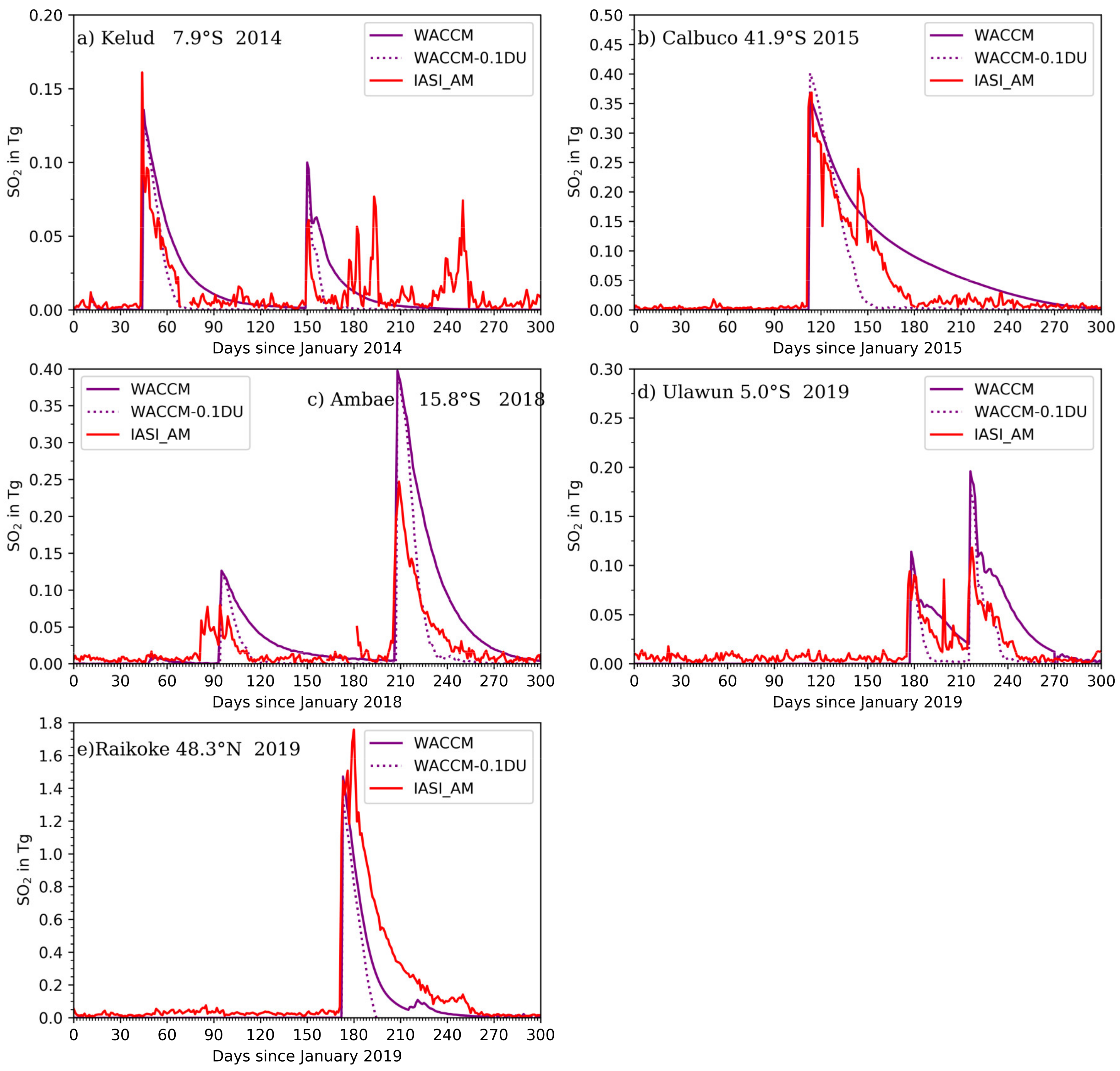
3.1. Temporal Evolution of the SO2 Burden

Figure 1 shows the modelled SO2 burden for each volcanic eruption, calculated by integrating the model anomalies (in teragrams) from WACCM simulations. For each event, the SO2 burden is shown in the region where the injection occurred, i.e., northern hemisphere (NH; 0–80° N), southern hemisphere (SH; 0–80° S) or tropics (20° S–20° N). Alongside is shown the observed evolution of SO2 burden derived from the IASI retrieval. Most of the peak burdens are correctly reproduced by the model but simulated SO2 generally tends to decline less rapidly than the IASI observations. This feature has already been observed in a similar study comparing WACCM outputs and IASI for the Sarychev eruption in 2009 and has been attributed to the greater dispersion of the SO2 plume transport in the coarse model grid cells than in reality [22,87]. In terms of peak amplitude, the model tends to largely overestimate IASI observations by 60% and 82% for the Ambae and Ulawun main injections, respectively. WACCM-CARMA shows underestimated SO2 peaks by 19 and 14% for the Kelud and Raikoke, respectively. The best agreement is obtained with the Calbuco case with a slight underestimation of 6% by the model.
The differences between WACCM and IASI in the SO2 column evolution can be quantified in terms of e-folding time corresponding to the time by which the concentration falls to 1/e of its initial value [22]. Results, summarized in Table 2 for all reported eruptions between 2013 and 2019, clearly show longer e-folding time derived from the model outputs for all the eruptions except for the Raikoke one. The e-folding values are quite disparate from one eruption to another. Carn et al. (2016) [88] have highlighted a correlation between the altitude of the SO2 injection and the lifetime of SO2. They have also suggested a related dependence of SO2 lifetime on the amount of injected SO2 and the latitude of injection which might explain the various e-folding times we have calculated in our study.
Too slow an oxidation time of SO2 in the model could be suggested to explain partly the differences with the IASI observations. However, as argued by Haywood et al. (2010) [87] and Lurton et al. (2018) [22], accounting for a detection limit in the IASI SO2 columns (a threshold below which SO2 amounts are not detected by the instrument) decrease the derived e-folding times. The higher the IASI detection limit, the faster the e-folding time decreases. The SO2 detection threshold of the new IASI algorithm is estimated to be around 0.1 DU, i.e., lower than the 0.3 DU value used in the former studies by Haywood et al. (2010) [87] and Lurton et al. (2018) [22]. Adjusting the WACCM-CARMA model outputs for a 0.1 DU SO2 lower value of the IASI retrieval clearly leads to a faster decay of the SO2 columns for all eruptions (Figure 1) and reduces the associated e-folding times, without however robustly matching the observed SO2 evolution, except for the Kelud case.
Specifically, for the Kelud case, we find a simulated e-folding time of ~18 days versus of value of ~26 days from the model set-up of Mills et al. (2016) [83]. Zhu et al. (2020) [86] have simulated an e-folding time of ~22 days for a simulation computing sulphate aerosols (with an uniform injection of SO2 between 17 and 26 km) and microphysical processes on ash. Ash particles emitted by the Kelud volcano have not been accounted for in our simulation. The reported presence of ash for the Kelud eruption has been shown to shorten the SO2 lifetime through uptake processes [86].
Zhu et al. (2020) [86] have shown that about 20% of the initial SO2 has been removed from the gas phase mostly during the first day of the eruption, with an uptake which typically saturates over time. Their simulations accounting for sulphur/ash microphysical processes and including SO2 uptake on ash better reproduces the temporal evolution of SO2 as observed from satellite instruments in the tropics, leading to a reduced modelled e-folding time of ~17 days. A similar value has been obtained from our simulation without including ash. Furthermore, accounting for the 0.1 DU detection threshold makes the model e-folding time match the value inferred from IASI. These are indications about the strong impact, perhaps dominating, of altitude ranges and areas of injection on the SO2 lifetime.
For the Raikoke, we find an average SO2 e-folding time of ~15 days whereas a value of 16 days is derived from IASI. A value of 14–15 days has been found de Leeuw et al. (2021) [89] using satellite observations from the TROPOspheric Monitoring Instrument (TROPOMI). The retrieved altitudes from IASI observations have shown large variations which affect the retrieval of the SO2 columns reflecting the complexity of this eruption. As discussed in Kloss et al. (2021) [41], differences between various observation sources in terms of injection sequence and altitude make it difficult to initialize properly the simulation for this specific event. The significant increase of the Raikoke SO2 lifetime suggested by IASI observations very likely implies a transport mechanism not represented in the model. The unambiguous presence of ash as detected from satellite observations [90] can have impacted the SO2 lifetime. However, as discussed above, the presence of ash is supposed to shorten the SO2 lifetime and this would even increase the difference between the simulations and IASI observations. The radiative heating effects due to the co-located presence of optically absorbing smoke particles emitted from wildfires in late spring and early summer 2019 is also under consideration by the VolRes community. Such radiative effects could have made the air masses rise to higher altitudes impacting the oxidation of SO2 [88].

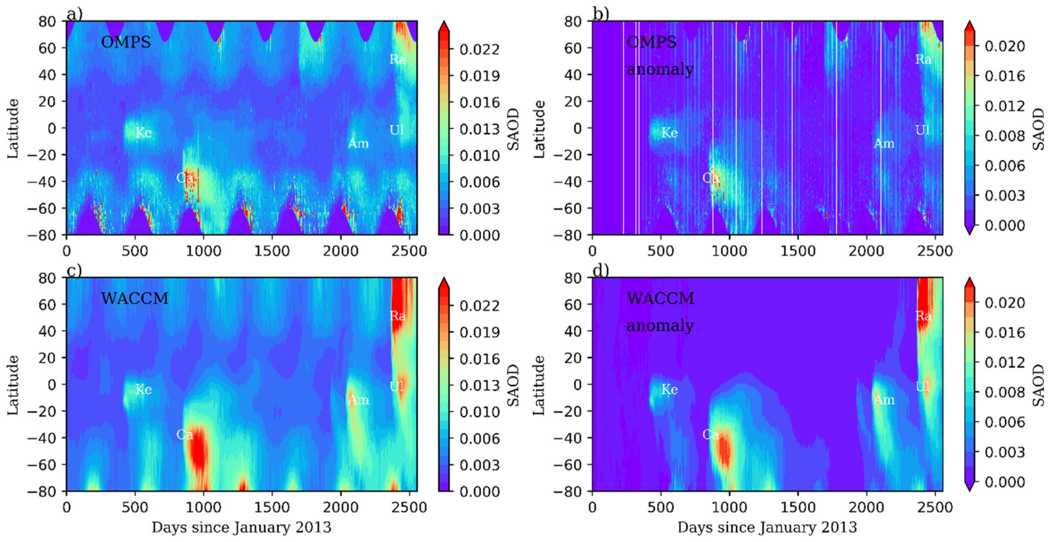
3.2. Modelled and Observed Space-Time Variability of the Stratospheric Aerosol Burden

3.2.1. The Kelud and Ambae Tropical Eruptions

Extinction data from satellite observations have been used for model and observational assessment of stratospheric aerosol impacts from moderate-magnitude volcanic eruptions in a number of studies [87,91], including the WACCM-CARMA model [22,41]. Figure 2 presents a time series of daily and zonal means of extinction coefficient at 675 nm in the tropics (20° S to 20° N) from 2013 to 2019 based on OMPS measurements and WACCM-CARMA simulations. OMPS extinction anomalies are calculated with respect to the 2013 volcanically quiescent year whereas WACCM-CARMA anomalies are derived from the volcano-on minus the volcano-off simulation. Note that WACCM-CARMA anomalies result in very similar values when calculated with respect to the year 2013 as done for OMPS. Overall, the simulated patches related to the formation of volcanic sulphuric acid aerosols match the positions of the bulk extinction patterns pointed out by OMPS in the stratosphere. The maximum vertical extents of the plumes seem also generally reproduced by the model both for the absolute values of extinctions and for anomalies.
Volcanic eruptions of the Kelud and Ambae volcanoes localized in the tropics show a clear signature in Figure 2 with a similar vertically propagating pattern in the observations and in the simulations. The upward transport of the Kelud and Ambae plumes reflects the “tape-recorder” effect, already highlighted by Vernier et al. (2011) [17] in former tropical eruptions and shows a more visible signal in OMPS observations. The modelled extinctions for the Kelud are ~25% higher (on average over the whole area covered by the plume) than the OMPS observed values. Around 15 km, we notice that a signature of high-altitude clouds is still present in the cloud-filtered OMPS data both in terms of absolute values of extinction (Figure 2a) and anomalies (Figure 2b).
The temporal distribution of zonally averaged SAOD for OMPS observations and WACCM-CARMA simulations for both hemispheres is presented in Figure 3. Here, again, observations and simulations show the same locations of the plumes. The intensity of the Kelud signal and its space-time extent seems well reproduced by the model (with ~6% differences on average over the whole areas covered by the plumes) both for absolute values of SAOD (Figure 3c) and anomalies (Figure 3d). The aerosol SAOD enhancement in the simulation between 40° S and 60° S is attributed to the propagation of the Kelud signal from the tropics to the SH mid-latitudes. This feature appears a bit less evident in OMPS SAOD observations but is more visible when observed extinction is integrated over lower altitude ranges (i.e., closer to the tropopause) to derive SAOD (not shown). The occurrence of such meridional transport would depend on the phase of the QBO [27,28] and the seasonal variations of the tropical dynamical barriers [24,92] which is not explored here.
The model–observation differences are very pronounced for the Ambae eruption both for the formation and decay phases of the aerosol plume. The WACCM-CARMA model shows much stronger extinction and SAOD with values ~200% higher than OMPS (Figure 2 and Figure 3). Some transport from tropical latitudes to the mid-latitude SH of the Ambae aerosol plume is simulated by the model (Figure 3c,d). However, as for the Kelud case, this is less clear in OMPS observed anomalies. Note that such transport features are more apparent if the OMPS SAODs are derived for maximum altitudes closer to the tropopause (not shown).
We note that the signal of the summer 2017 Canadian wildfires is visible in OMPS data in the northern hemisphere (Figure 3). Kloss et al. (2019) [40] have reported that a small part of the fire plume was transported towards tropical latitudes via the Asian monsoon anticyclone circulation but its signature is not visible in the zonally averaged extinctions presented in Figure 2. No smoke aerosols from the Canadian fires have been computed in our WACCM-CARMA simulation conversely to the work of Yu et al. (2019) [93].
Integrating the SAOD data on latitudinal bands provides another insight into the differences between the observations and the simulations (Figure 4a). Overall, the average difference for SAOD between WACCM-CARMA and OMPS after the sulphur injection is of 5.8% for Kelud. The evolution of integrated SAOD of the Kelud eruption shows a faster increase in the model at an early stage of the formation of the aerosol plume and a very similar behaviour between OMPS and WACCM-CARMA during the decay phase (Figure 4a). Only about 60 days after the eruption, the model and observations agree well in terms of absolute values of SAOD. The results of Zhu et al. (2020) [86] show a zonally averaged modelled aerosol content within 20% of CALIOP values between 20 and 60 days after the Kelud eruption when considering sulphur/ash interactions. In this case, the sulphate production is largely controlled when including SO2 chemical reaction on ash surfaces rather than the direct removal of sulphate and H2SO4 gas (i.e., through heterogeneous nucleation and coagulation processes) by ash, significantly impacting the temporal evolution of the sulphate burden. Based on these results of Zhu et al. (2020) [86] (see their Figure 6b), we would expect faster production of sulphate (than SO2 oxidation to sulphate in the gas phase) over the first days of the plume formation but a flattened evolution and reduced maximum values of SAOD over the first 60-day period after the Kelud eruption.
We note from Figure 4a that the SAOD from the volcano-off simulation over the period prior to the Kelud injection is higher than the values observed by OMPS perhaps reflecting some difficulty of the model to simulate the background aerosol content.
The SAOD simulated for the Ambae eruptions is strongly overestimated when compared to the OMPS record (Figure 4c) resulting in an averaged difference between WACCM-CARMA and OMPS of 202% for the period following the sulphur injection. Results for this specific event may reflect an inaccurate knowledge of the SO2 burden (as seen from the comparison with IASI in Figure 1) as well as injection timing and altitude for an eruption which was not widely reported in the literature.

3.2.2. The Calbuco Eruption and Its Impact on the Tropics

The Calbuco plume, though injected in the SH mid-latitudes, has shown a clear signal propagating to the tropics as observed from ground-based and spaceborne instruments [39,94] which is further confirmed by the OMPS observations and WACCM-CARMA simulations in Figure 3. The latitudinal extent within the tropics has been shown to be clearly bounded by the subtropical barrier [24]. The space-time extent of the Calbuco plume seems rather well reproduced by WACCM-CARMA (if we exclude the observed presence of clouds) although absolute values of mean extinction are overestimated by ~25% by the model (Figure 2) and by ~100% for SAOD (Figure 3). The volcanic aerosol signal, lasting until summer 2016, is more pronounced in the model than in OMPS. The anomalies shown in Figure 2b and Figure 3b indicate that a remaining slight signal of the Kelud from OMPS observations may have interfered with the one of the Calbuco on a zonal average basis whereas the model outputs do not indicate any overlapping between the two plumes from Figure 2d and Figure 3d. The remaining signature of the Kelud plume is visible from the simulated SAOD evolution in the tropics shown in Figure 4b with a calculated Kelud signal of less than 2 × 10⁻³ prior to the Calbuco injection. We note that the most significant aerosol signal has propagated in the poleward direction which has tended to strengthen the formation of polar stratospheric clouds in the Antarctic polar vortex [16]. The Calbuco aerosols are still present in the southern hemisphere mid-latitudes about one year after the eruption.
The observed and simulated evolutions of SAOD integrated over the SH and the tropics for Calbuco match well during the increase phase, i.e., when the sulphuric acid aerosols form (Figure 4b). The model computes higher integrated SAOD values during the decay period when the aerosols are transported and removed from the stratosphere. The averaged difference in SH SAOD between the model and the observations is of 111% for Calbuco. In the tropics, the simulated SAODs remain higher than the OMPS record following the volcanic injection with a model signal even tending to increase until the end of the year 2015, resulting in an averaged model–observation difference of 28% whereas a rather steady feature is observed by OMPS.
Differences between WACCM-CARMA and satellite observations in terms of SAOD evolution have already been reported by Lurton et al. (2018) [22] for the midlatitude Sarychev eruption in 2009 and have been partly attributed to a bias in the sampling of the OSIRIS version 5.07 datasets. Since then, sampling issues have been addressed with the release of OSIRIS version 7 [95]. As discussed by Kloss et al. (2021) [41], differences between model and OMPS observations may be partly attributed to sampling issues since the model outputs are provided globally twice a day whereas OMPS reaches a global coverage every ~3 days.

3.2.3. The Raikoke and Ulawun Eruptions in Summer 2019

The mid-latitude Raikoke eruption has been reported as the largest volcanic event since 1991 Mount Pinatubo eruption in terms of produced aerosol burden in the stratosphere. As shown by Kloss et al. (2021) [41], the plume mainly extended throughout the NH mid- and high latitudes but some part was transported to the tropics. Both tropical Ulawun eruptions occurred around the same period and their signal in the 20° S–20° N latitude band cannot be distinguished from the Raikoke one on a zonal view, both in the satellite and the model data (Figure 2). Figure 3 confirms the propagating pattern of the Raikoke plume from mid-latitudes to the tropics and the subsequent mixing of both volcanic plumes. Differences of ~150% are calculated between WACCM-CARMA and OMPS for extinction and SAOD (Figure 2 and Figure 3). We also note that for the period before the Raikoke eruption, the simulated signal is higher than the “background” one probably as a result of the remaining aerosols from the Ambae eruption (Figure 4d,e).
As reported by Kloss et al. (2021) [41], significant differences can be observed between OMPS and WACCM-CARMA for absolute values of extinction and for the space-time evolution of the plumes. This feature is reflected in the SAOD evolution shown in Figure 4d), especially during the early stage of the Raikoke plume formation (i.e., the first ~40 days after the eruption). The simulated SAODs tend to increase faster than the observed record, mirroring a stronger and faster formation of sulphuric acid aerosols in the model and showing a shorter decay. Averaged differences of 112% and 130% are calculated between WACCM-CARMA and OMPS for the period following the sulphur injection for Raikoke in the NH (Figure 4d) and Raikoke+Ulawun in the tropics (Figure 4e), respectively. This translates into differences in SAOD e-folding times (Table 2).
Sensitivity tests have been conducted to investigate the reasons for the model–OMPS discrepancies for the Raikoke plume. Modifying the altitude and timing of injection in the model set-up does not reduce significantly the differences in the aerosol content, the model still calculates a faster aerosol production during the weeks following the eruption (not shown). The injection of 1.5 Tg of SO2 seems a correct value among the various published and ongoing studies regarding this eruption (e.g., [89] and see VolRes initiative). As discussed for the Kelud eruption, the collateral presence of ash is expected to decrease the SO2 lifetime as well as the maximum sulphate SAOD values. An enhanced difference between IASI SO2 and WACCM-CARMA due to chemical and microphysical action of ash does not satisfactorily explain the OMPS-model discrepancy for aerosol extinction and SAOD, at least in the chosen model set-up of our work. However, Muser et al. (2020) [90] have shown evidence that aerosol–radiation interactions in presence of ash have impacted the dispersion of the Raikoke plume. This process has favoured the rise of the plume a few days after the eruption, higher up than simulated by the model, especially if smoke particles from wildfires were simultaneously present. As a result, we cannot exclude issues in the calculation of transport by the model if optically absorbing particles are not accounted for. This also suggests that our vertical range of injection may be not adequate. Finally, an injection of water in the stratosphere by the Raikoke volcano can have enhanced the OH production and then reduced the SO2 lifetime once again reinforcing the model–IASI difference. This hypothesis may be not plausible as large amounts of injected water would be necessary to reduce significantly the sulphate aerosol content as tested for the Kelud eruption [86]. The reason for the model–observation discrepancy is still to be determined. For the Ulawun case, we suspect that the information about the injection parameters (amount of SO2, altitude, timing) is not sufficiently accurate.

3.3. Comparisons of Model Simulations and In Situ Balloon-Borne Observations in the Tropics

3.3.1. Observations of the Kelud Plume from Darwin, Australia

During the first ten days after the eruption of the Kelud volcano of 13 February 2014, space-borne observations from CALIOP have revealed a maximum extinction signal at 20 km [85], i.e., the altitude of injection of sulphur computed in the WACCM-CARMA model. A significant signature of ash in the Kelud plume was observed by CALIOP, peaking in the ~18.5–19.5 km altitude range, i.e., below the maximum signal of sulphate at 20 km, with extinction values and altitude of ash decreasing with time. About three months after the Kelud eruption, aerosol profile measurements were conducted during the KlAsh (Kelud-Ash; https://science.larc.nasa.gov/KLASH/; accessed on 1 June 2021) field campaign in May 2014 in the area of Darwin, northern Australia (12.4° S, 130.8° E), using the COBALD and LPC in situ balloon-borne instruments [85].
Figure 5 presents four extinction profiles derived from COBALD backscatter observations using a lidar ratio of 45sr+/−10 calculated by averaging typical sulphate and ash lidar ratios of 50 sr and 40 sr, respectively, [85]. The signal at the 532 nm lidar wavelength has been interpolated using the Angström exponent deduced from the LED wavelength of 455 nm and 940 nm. The WACCM-CARMA model outputs agree well with COBALD observations by remaining within the uncertainty range. Below 20 km COBALD observations reflect some short-term variability which is partially captured by the model. However, comparisons with WACCM-CARMA show overall good agreement in terms of profile shape and peak altitude 3 months after the eruption, i.e., a period during which observed and simulated AOD agree well (Figure 4a). At the period of the KlAsh campaign, the average signal due to ash detected by CALIOP in the tropics (20° S–20° N) was much weaker than at an early stage of the plume with an ash fraction both estimated from CALIOP and LPC observations of 20–25% of AOD (excluding the contribution from background aerosols) [85]. This may explain why computing sulphate only appears sufficient for WACCM-CARMA to reproduce the observed extinction profiles in May 2014.
Observations of the optical properties and of size distributions by the ULPC on 20 May 2014 show a dominant contribution of non-volatile particles (most likely associated with ash) below 20 km for sizes greater than ~0.5 µm but volatile particles associated with sulphuric acid largely dominate in terms of total concentration for the whole altitude range [85].
Figure 6a,b show both the model and measured aerosol particle number concentrations for two particle size ranges: radii (r) > 10 nm and r > 150 nm. The measurements for r > 10 nm are made with CN counter and above 75 nm with an LPC. There is very good agreement between simulated and measured values in terms of total number concentrations and variation with respect to altitude indicating that nucleation and coagulation processes of stratospheric aerosols are well captured by the model as already pointed out by English et al. (2011) [69]. Note that model–measurement differences are greater in the troposphere since only sulphuric acid particles are simulated. For particles with r > 150 nm, the particle concentrations increase by a factor of ~6 with respect to the volcano-off simulation at the altitudes of the profile peak. The volcano-on simulated profile shows rather good agreement for maximum concentration values and overall reproduces well the shape of the profile. However, it shows a wider plume peak and tends to significantly overestimate the observed profile above the peak. Differences may arise from uncertainties in the initialization altitude and from the coarser model resolution which can lead to an anomalous sulphate plume structure over the measurement location as highlighted for a similar comparison exercise for the Sarychev volcanic plume in 2009 [22].

3.3.2. Observations of the Calbuco Plume over la Reunion Island

The Calbuco plume has been investigated from ground-based lidar, in situ balloon-borne OPC and satellite observations at la Reunion Island (Maïdo Observatory; Maido, France; 20.5° S, 55.5° E) in the framework of the MORGANE campaign. Details about the various instruments and the long-range transport characteristics of the plume from the location of its emission to the tropics can be found in Bègue et al. (2017) [24].
The LOAC OPC was launched on 19 May 2015 about one month after the eruption. A second flight was conducted on 19 August 2015 to explore the decay of the volcanic plume. Both concentration profiles are compared to WACCM-CARMA outputs at the grid point closest to the observation (Figure 7a). On 19 May, the particle concentrations increase by a factor of ~10 with respect to the volcano-off simulation at the altitudes of the profile maximum. The observed signature of the Calbuco plume is peaking at ~17.5 km which is reproduced by the model. Concentrations simulated by WACCM-CARMA at the altitude of the peak are a factor of ~10 lower than values observed by the OPC. Above, at altitude levels not impacted by the volcanic aerosols, the difference can reach a factor of more than 10 and concentration values observed by the LOAC OPC at these altitudes strongly exceed the concentrations in “background” conditions in the tropics [24]. Note that comparisons using other model grid points show similar differences (not shown).
On 19 August, locally the Calbuco plume had spread out vertically and the model show an increase of a factor of ~5 when volcanic aerosols are present (Figure 7b). Good agreement is observed between the model and the OPC, except above 25 km where the measured increase is not reproduced by the model. Such a high altitude feature has been occasionally observed and has not been yet clearly attributed to a specific phenomenon [6,96]. We note that the WACCM-OPC discrepancies on the concentration values do not match the WACCM-OMPS SAOD differences showing better agreement on 19 May than on 19 August 2015 (Figure 4).
Figure 8 depicts the evolution of the 532-nm SAOD calculated between 17 and 30 km from lidar observations at Reunion Island (Maïdo Observatory; 20.5° S, 55.5° E), from OMPS satellite overpasses within a 10° × 10° latitude and longitude grid around the lidar site and from the WACCM-CARMA volcano-on simulation between 1 April 2014 and 1 January 2017. Wavelength conversion from 675 and 532 nm has been conducted using Angström exponents [47], similarly to Bègue et al. (2017) [24].
A sharp increase in the stratospheric aerosol loading was observed above la Reunion a few weeks after the Calbuco eruption, with SAOD values increasing by a factor of 2–3 in the observed records with respect to the beginning of 2014 and by a factor of ~4 in comparison with the end of 2016. Overall good agreement is observed between the various datasets in the occurrence of the maximum Calbuco signal above la Reunion and decay trend. In late 2016, the aerosol content seemed back to “background” conditions which is similarly captured by the various datasets. The significant short term (i.e., daily) variability in the lidar observations and in the model outputs reflects a transient behaviour of the aerosol layers above la Reunion Island and inhomogeneous spatio-temporal distribution of the Calbuco plume controlled by the fluctuations of the subtropical dynamical barrier [24]. This may partly explain the differences between model and in situ observations in Figure 7a. Some periods show some discrepancies in terms of SAOD absolute values with the model tending to overestimate SAOD with respect to observations around day 300, and between 400 and 700 days after the eruption. At the period of the first LOAC OPC observations (around day 414), the simulations and the other datasets show very variable SAOD reflecting the presence of transient layers (with possible filamentary structures) highlighted by Bègue et al. (2017) [24].
During the period before the Calbuco pulse, the aerosol content showed more variability and higher levels than in late 2016 possibly due to some remaining signature of the Kelud aerosols estimated to be of ~3.10–3 from OMPS zonally averaged anomalies (Figure 2 and Figure 3) for days 0–200, i.e., close to the background values of 4.10–3 shown for day 1000. Discrepancies between OMPS and other datasets may be partly explained by the different geographical areas used to derive SAOD.

4. Conclusions

In this study we have analysed five moderate-amplitude volcanic eruptions which have impacted the stratospheric aerosol burden in the tropics over the 2013–2019 period, largely exceeding the signal of stratospheric aerosols under unperturbed conditions. Simulations with the WACCM(CESM1)-CARMA model have been used to investigate the variability and transport characteristics of the sulphate plumes produced from SO2 injections. Three of these volcanoes (Kelud in 2014, Ambae in 2018 and Ulawun in 2019) have directly injected material in the tropical stratosphere whereas two other ones (Calbuco in 2015 and Raikoke in 2019) are localized in extra-tropical latitudes with material subsequently transported to the tropics. The model has been driven from information available in the literature or from scientific communications in terms of SO2 burden, altitude range and time of injection. The timing of the SO2 column decay shows some differences between WACCM-CARMA simulations and IASI space-borne observations, with the model decreasing slower than the measurement for most of the eruptions, a feature already observed for the 2009 Sarychev mid-latitude plume [22]. Adjusting the WACCM-CARMA model outputs for a detection limit value of 0.1 DU SO2 of the IASI retrievals leads to a faster decay of the simulated columns, leading to underestimation by the model. The comparison for the Raikoke shows a different behaviour with the model decreasing faster in all cases. The simulated and observed amplitudes of the SO2 peaks do not perfectly match for some eruptions (especially for the Ambae and Ulawun) possibly due to inaccurate information available in the literature. Finally, the various e-folding times among the eruptions may indicate a dependence of the SO2 lifetime to the latitude of injection [88].
Although WACCM-CARMA simulations tend to reproduce OMPS observations for the spatial extent of the plumes (on a zonal average basis), significant differences are shown in terms of absolute values of aerosol burden (extinction and SAOD) especially for the Ambae, Raikoke and Ulawun eruptions, indicating again that the information on the injection parameters available for some of these eruptions should be reconsidered. These discrepancies are not explained by the 20% relative accuracy and precision of OMPS 675 nm extinction [39]. We did not find evidence of any bias in OMPS SAOD (missing values in the vertical profile of extinction leading to biased calculated SAOD and saturation effect above a certain value of extinction) as reported by Lurton et al. (2018) for other satellite data.
Model-measurement discrepancies are likely to arise from different sources of uncertainties related to the complex interplay between injection parameters, dynamics and chemistry specific to each plume. The knowledge of the injection timing (especially if the eruption is characterized by a series of pulses, i.e., multiple injections) and altitude ranges to drive models is of high importance for the SO2 lifetime and aerosol plume evolution. However, altitudes of SO2 injection are likely to differ between various satellite observations [41] due to insufficient vertical resolution, affecting the mass distribution estimate of SO2 relative to the tropopause. The horizontal extent of the SO2 injection can be a factor limiting the ability of the model to match the observations and the coarser model horizontal resolution can lead to an anomalous sulphate plume structure [22]. While we have chosen to inject the sulphur on a given model grid point (closest to the volcano location), Zhu et al. (2020) [86] have spread the injection over a given latitude-longitude band in order to capture enough wind shear to reproduce the horizontal SO2 patterns observed by the satellite instrument. This configuration, as well as increasing the horizontal resolution of the simulations, could be tested in the future. Another way of improving the model initialisation would be to use profiles of SO2 reconstructed by the combination of space-borne observations of SO2 column and vertically resolved aerosol profiles (from CALIOP) using [97]. Finally, using WACCM-CARMA in the free-running mode with different weight factors towards different operational analyses or reanalyses (e.g., MERRA2, ERA-5, JRA-55) which have shown some discrepancies in the representation of stratospheric winds [98,99,100] could be interesting tests to investigate the model ability to simulate stratospheric transport and the impact on volcanic plume dynamics (hemispheric spreading, meridional transport towards the tropics, vertical motion driven by the BDC, effects of dynamical barriers and of the QBO, phase, etc.).
Comparisons of the model outputs with in situ observations show contrasting results and illustrate issues with the horizontal and vertical resolutions differing between the datasets. Good agreement is obtained with the aerosol content COBALD backscatter sondes (extinction) and the LPC (concentrations) in the layers impacted by the Kelud plume. For the Calbuco aerosols, strong differences are shown between the WACCM simulations and LOAC OPC measurements at an early stage of the plume propagation (~4 weeks after the initial injection) whereas good agreement is observed at the period when the plume has spread throughout the SH (~4 months after). This result is also reflected in the comparisons with lidar observations from la Reunion Island and illustrates the difficulty of the model to simulate transient aerosol structures with a more local scale. Peak altitude differences between the model and in situ data can be caused by the mismatch of the vertical resolution of the model which is ~1 km in the stratosphere as well as inaccuracy in the injection parameters. For altitude levels free of volcanic influence, the model clearly shows some discrepancies with in situ observed concentrations, demonstrating the difficulty of the model to simulate the “background” aerosol content in the accumulation mode, whereas comparisons using parameters integrating the whole aerosol size spectrum (such as total concentrations and extinction) interestingly show good agreement.
The co-injection of ash is likely to play a significant role in aerosol production and plume evolution through uptake of SO2 [86]. The presence of ash has been reported for the Kelud eruption [85,86] and could explain why the WACCM-CARMA outputs overestimate the SAOD over the first few weeks after the emission (if we assume that the injection parameters used to drive the simulation are correct). For the Raikoke plume, some evidence about the presence of ash has been recently highlighted [90,91] and, following the work of Zhu et al. (2020) [86], its effect on the simulated aerosol evolution needs to be investigated, although one would expect increased differences between simulated and observed SO2 in this case, pointing out the specificity of this eruption. At this stage, significant contributions of ash from the other eruptions investigated in our study have not been reported yet in the literature. Aerosol–radiation interaction when optically absorbing ash (and possibly smoke particles emitted by fires in summer) is present may also be a major factor driving the plume dynamics and need to be investigated.
Finally, this study highlights some difficulties for our global model simulations in reproducing volcanic plumes for various reasons proposed above. The case study of the 2009 Sarychev plume previously reported by Lurton et al. (2018) [22] using WACCM-CARMA has shown good agreement with observations using a simple injection sequence but our results tend to indicate that this strategy may be not appropriate for each event. Combining various space-borne observations to catch the whole injection sequence are a prerequisite to robustly drive and assess model simulations. Furthermore, in situ observations using light balloons regularly conducted along the periods impacted by volcanic plumes owing to their high operational flexibility, would be particularly valuable to assess the model in terms of microphysical processes.

Author Contributions

Writing-original draft preparation, investigation, software, visualization, M.T.; methodology, supervision, funding acquisition, G.B. and F.J.; investigation and analysis of OMPS satellite data, C.K.; design of the LOAC instrument, data processing, investigation and analysis of in situ aerosol data, J.-B.R.; PI of the KlAsh Campaign, investigation and analysis of in situ balloon-borne aerosol data, J.-P.V.; investigation of model outputs and software, A.B.; methodology, investigation of IASI SO2 data, IASI data curation, L.C.; OMPS data processing, investigation of OMPS data, G.T.; design and PI of the LPC balloon-borne instrument, data processing and analysis, investigation, T.D.; processing and analysis of COBALD data, formal analysis, Methodology, F.G.W.; processing and investigation of lidar data, data curation, N.B., T.P., S.G.-B., G.P., V.D. and N.M.; balloon operations in la Réunion Island during the MORGANE campaign, J.-M.M. All authors have read and agreed to the published version of the manuscript.

Funding

This research was funded by the VOLTAIRE project (ANR-10-LABX-100-01) funded by ANR through the PIA (Programme d’Investissement d’Avenir), in particular through the IANU sub-project, is gratefully acknowledged. The authors are grateful for the support of Agence Nationale de La Recherche under grant ANR-17-CE01-295 0015 (TTL-Xing). The KLASH campaign was funded by the NASA Rapid Response and Novel Research in Earth Science. The authors acknowledge the European Communities, the Région Réunion, CNRS and Université de la Réunion for their support and contributions in the construction phase of the research infrastructure OPAR (Observatoire de Physique de l’Atmosphère de La Réunion) and the Bureau of Meteorology. OPAR is presently funded by CNRS (INSU) and Université de La Réunion and managed by OSU-R (Observatoire des Sciences de l’Univers de La Réunion, UAR 3365). Corinna Kloss was funded by the Deutsche Forschungsgemeinschaft (DFG, German Research Foundation)—409585735.

Data Availability Statement

The aerosol extinction dataset from OMPS v2 are available at https://daac.gsfc.nasa.gov/ (accessed on 27 November 2021). IASI Level 1c data are provided by the AERIS/ICARE data center (https://en.aeris-data.fr/direct-access-icare/ (accessed on 27 November 2021)) and may be requested from Lieven Clarisse for updated versions. LOAC in situ aerosol data are available in open access at https://zenodo.org/record/5918581#.YfV2vudCdEY (accessed on 27 November 2021). LPC in situ aerosol data are available in open access at ftp://cat.uwyo.edu/pub/permanent/balloon/Aerosol_InSitu_Meas/AU_Darwin_13S_132E/ (accessed on 27 November 2021). Lidar data have to be requested from Nelson Bègue. The model and simulation outputs may be requested from the corresponding author.

Acknowledgments

The authors wish to thank the CaSciModOT structure (Calcul Scientifique et Modélisation Orléans-Tours), part of the French national network of complex systems (RNSC–Réseau National des Systèmes Complexes), thanks to which the simulations could be completed. KLASH was a collaborative effort between NASA LaRC, the University of Wyoming and ETH. Mariam Tidiga would also like to thank the NCAR/CESM online discussion board for many helpful technical discussions that helped throughout this study.

Conflicts of Interest

The authors declare no conflict of interest. The funders had no role in the design of the study; in the collection, analyses, or interpretation of data; in the writing of the manuscript, or in the decision to publish the results.

References

  1. Haywood, J.M.; Jones, A.; Jones, G.S. The impact of volcanic eruptions in the period 2000-2013 on global mean temperature trends evaluated in the HadGEM2-ES climate model. Atmos. Sci. Lett. 2014, 15, 92–96. [Google Scholar] [CrossRef] [Green Version]
  2. Monerie, P.A.; Moine, M.P.; Terray, L.; Valcke, S. Quantifying the impact of early 21st century volcanic eruptions on global-mean surface temperature. Environ. Res. Lett. 2017, 12, 054010. [Google Scholar] [CrossRef] [Green Version]
  3. Neely, R.R.; Toon, O.B.; Solomon, S.; Vernier, J.P.; Alvarez, C.; English, J.M.; Rosenlof, K.H.; Mills, M.J.; Bardeen, C.G.; Daniel, J.S.; et al. Recent anthropogenic increases in SO2 from Asia have minimal impact on stratospheric aerosol. Geophys. Res. Lett. 2013, 40, 999–1004. [Google Scholar] [CrossRef]
  4. Kremser, S.; Thomason, L.W.; von Hobe, M.; Hermann, M.; Deshler, T.; Timmreck, C.; Toohey, M.; Stenke, A.; Schwarz, J.P.; Weigel, R.; et al. Stratospheric aerosol—Observations, processes, and impact on climate. Rev. Geophys. 2016, 54, 278–335. [Google Scholar] [CrossRef]
  5. Murphy, D.M.; Froyd, K.D.; Schwarz, J.P.; Wilson, J.C. Observations of the chemical composition of stratospheric aerosol particles. Q. J. R. Meteorol. Soc. 2014, 140, 1269–1278. [Google Scholar] [CrossRef]
  6. Renard, J.B.; Berthet, G.; Levasseur-Regourd, A.C.; Beresnev, S.; Miffre, A.; Rairoux, P.; Vignelles, D.; Jégou, F. Origins and spatial distribution of non-pure sulfate particles (Nsps) in the stratosphere detected by the balloon-borne light optical aerosols counter (loac). Atmosphere 2020, 11, 31. [Google Scholar] [CrossRef]
  7. McCormick, M.P.; Thomason, L.W.; Trepte, C.R. Atmospheric effects of the Mt Pinatubo eruption. Nature 1995, 373, 399–404. [Google Scholar] [CrossRef]
  8. Robock, A. Volcanic eruptions and climate. Rev. Geophys. 2000, 38, 191–219. [Google Scholar] [CrossRef]
  9. Arfeuille, F.; Weisenstein, D.; MacK, H.; Rozanov, E.; Peter, T.; Brönnimann, S. Volcanic forcing for climate modeling: A new microphysics-based data set covering years 1600-present. Clim. Past 2014, 10, 359–375. [Google Scholar] [CrossRef] [Green Version]
  10. Solomon, S. Stratospheric ozone depletion: A review of concepts and history. Rev. Geophys. 1999, 37, 275–316. [Google Scholar] [CrossRef]
  11. Canty, T.; Mascioli, N.R.; Smarte, M.D.; Salawitch, R.J. An empirical model of global climate-Part 1: A critical evaluation of volcanic cooling. Atmos. Chem. Phys. 2013, 13, 3997–4031. [Google Scholar] [CrossRef] [Green Version]
  12. Soden, B.J.; Wetherald, R.T.; Stenchikov, G.L.; Robock, A. Global cooling after the eruption of Mount Pinatubo: A test of climate feedback by water vapor. Science 2002, 296, 727–730. [Google Scholar] [CrossRef] [Green Version]
  13. Oman, L.; Robock, A.; Stenchikov, G.; Schmidt, G.A.; Ruedy, R. Climatic response to high-latitude volcanic eruptions. J. Geophys. Res. Atmos. 2005, 110, 1–13. [Google Scholar] [CrossRef]
  14. Kravitz, B.; Robock, A.; Bourassa, A. Negligible climatic effects from the 2008 Okmok and Kasatochi volcanic eruptions. J. Geophys. Res. 2010, 115, D00L05. [Google Scholar] [CrossRef] [Green Version]
  15. Berthet, G.; Jégou, F.; Catoire, V.; Krysztofiak, G.; Renard, J.B.; Bourassa, A.E.; Degenstein, D.A.; Brogniez, C.; Dorf, M.; Kreycy, S.; et al. Impact of a moderate volcanic eruption on chemistry in the lower stratosphere: Balloon-borne observations and model calculations. Atmos. Chem. Phys. 2017, 17, 2229–2253. [Google Scholar] [CrossRef] [Green Version]
  16. Zhu, Y.; Toon, O.B.; Kinnison, D.; Harvey, V.L.; Mills, M.J.; Bardeen, C.G.; Pitts, M.; Bègue, N.; Renard, J.B.; Berthet, G.; et al. Stratospheric Aerosols, Polar Stratospheric Clouds, and Polar Ozone Depletion After the Mount Calbuco Eruption in 2015. J. Geophys. Res. Atmos. 2018, 123, 12308–12331. [Google Scholar] [CrossRef]
  17. Vernier, J.P.; Thomason, L.W.; Pommereau, J.P.; Bourassa, A.; Pelon, J.; Garnier, A.; Hauchecorne, A.; Blanot, L.; Trepte, C.; Degenstein, D.; et al. Major influence of tropical volcanic eruptions on the stratospheric aerosol layer during the last decade. Geophys. Res. Lett. 2011, 38, 1–8. [Google Scholar] [CrossRef] [Green Version]
  18. Solomon, S.; Daniel, J.S.; Neely, R.R.; Vernier, J.P.; Dutton, E.G.; Thomason, L.W. The persistently variable “background” stratospheric aerosol layer and global climate change. Science 2011, 333, 866–870. [Google Scholar] [CrossRef] [Green Version]
  19. Ridley, D.A.; Solomon, S.; Barnes, J.E.; Burlakov, V.D.; Deshler, T.; Dolgii, S.I.; Herber, A.B.; Nagai, T.; Neely, R.R.; Nevzorov, A.V.; et al. Total volcanic stratospheric aerosol optical depths and implications for global climate change. Geophys. Res. Lett. 2014, 41, 7763–7769. [Google Scholar] [CrossRef] [Green Version]
  20. Diallo, M.; Ploeger, F.; Konopka, P.; Birner, T.; Müller, R.; Riese, M.; Garny, H.; Legras, B.; Ray, E.; Berthet, G.; et al. Significant Contributions of Volcanic Aerosols to Decadal Changes in the Stratospheric Circulation. Geophys. Res. Lett. 2017, 44, 10780–10791. [Google Scholar] [CrossRef]
  21. Jégou, F.; Berthet, G.; Brogniez, C.; Renard, J.B.; François, P.; Haywood, J.M.; Jones, A.; Bourgeois, Q.; Lurton, T.; Auriol, F.; et al. Stratospheric aerosols from the Sarychev volcano eruption in the 2009 Arctic summer. Atmos. Chem. Phys. 2013, 13, 6533–6552. [Google Scholar] [CrossRef] [Green Version]
  22. Lurton, T.; Jégou, F.; Berthet, G.; Renard, J.B.; Clarisse, L.; Schmidt, A.; Brogniez, C.; Roberts, T.J. Model simulations of the chemical and aerosol microphysical evolution of the Sarychev Peak 2009 eruption cloud compared to in situ and satellite observations. Atmos. Chem. Phys. 2018, 18, 3223–3247. [Google Scholar] [CrossRef] [Green Version]
  23. Carslaw, K.C.; Kärcher, B. Stratospheric aerosol processes. In Assessment of Stratospheric Aerosol Properties (ASAP); SPARC Report N°4; Thomason, L., Peter, T., Eds.; World Climate Research Programme (WCRP): Zurich, Switzerland, 2006; Volume 124, pp. 1–152. [Google Scholar]
  24. Bègue, N.; Vignelles, D.; Berthet, G.; Portafaix, T.; Payen, G.; Jégou, F.; Benchérif, H.; Jumelet, J.; Lurton, T.; Renard, J.B.; et al. Long-range transport of stratospheric aerosols in the Southern Hemisphere following the 2015 Calbuco eruption. Atmos. Chem. Phys. 2017, 17, 15019–15036. [Google Scholar] [CrossRef] [Green Version]
  25. Portafaix, T.; Morel, B.; Bencherif, H.; Baldy, S.; Godin-Beekmann, S.; Hauchecorne, A. Fine-scale study of a thick stratospheric ozone lamina at the edge of the southern subtropical barrier. J. Geophys. Res. Atmos. 2003, 108, 4196. [Google Scholar] [CrossRef] [Green Version]
  26. Holton, J.R.; Haynes, P.H.; Mcintyre, M.E.; Douglass, A.R.; Rood, B. Stratosphere-troposphere exchange. Rev. Geophys. 1995, 33, 403–439. [Google Scholar] [CrossRef]
  27. Trepte, C.R.; Hitchman, M.H. Tropical stratospheric circulation deduced from satellite aerosol data. Nature 1992, 355, 626–628. [Google Scholar] [CrossRef]
  28. Baldwin, M.P.; Gray, L.J.; Dunkerton, T.J.; Hamilton, K.; Haynes, P.H.; Randel, W.J.; Holton, J.R.; Alexander, M.J.; Hirota, I.; Horinouchi, T.; et al. The quasi-biennial oscillation. Rev. Geophys. 2001, 39, 111–129. [Google Scholar] [CrossRef]
  29. Pitari, G.; Di Genova, G.; Mancini, E.; Visioni, D.; Gandolfi, I.; Cionni, I. Stratospheric aerosols from major volcanic eruptions: A composition-climate model study of the aerosol cloud dispersal and e-folding time. Atmosphere 2016, 7, 75. [Google Scholar] [CrossRef] [Green Version]
  30. Vernier, J.P.; Pommereau, J.P.; Garnier, A.; Pelon, J.; Larsen, N.; Nielsen, J.; Christensen, T.; Cairo, F.; Thomason, L.W.; Leblanc, T.; et al. Tropical Stratospheric aerosol layer from CALIPSO Lidar observations. J. Geophys. Res. Atmos. 2009, 114, 1–12. [Google Scholar] [CrossRef] [Green Version]
  31. Kloss, C.; Sellitto, P.; Legras, B.; Vernier, J.P.; Jégou, F.; Venkat Ratnam, M.; Suneel Kumar, B.; Lakshmi Madhavan, B.; Berthet, G. Impact of the 2018 Ambae Eruption on the Global Stratospheric Aerosol Layer and Climate. J. Geophys. Res. Atmos. 2020, 125, 403–439. [Google Scholar] [CrossRef]
  32. Pitari, G.; Cionni, I.; Di Genova, G.; Visioni, D.; Gandolfi, I.; Mancini, E. Impact of stratospheric volcanic aerosols on age-of-air and transport of long-lived species. Atmosphere 2016, 7, 149. [Google Scholar] [CrossRef] [Green Version]
  33. Clerbaux, C.; Boynard, A.; Clarisse, L.; George, M.; Hadji-Lazaro, J.; Herbin, H.; Hurtmans, D.; Pommier, M.; Razavi, A.; Turquety, S. Monitoring of atmospheric composition using the thermal infrared IASI/MetOp sounder. Atmos. Chem. Phys. 2009, 9, 6041–6054. [Google Scholar] [CrossRef] [Green Version]
  34. Clarisse, L.; Coheur, P.F.; Theys, N.; Hurtmans, D.; Clerbaux, C. The 2011 Nabro eruption, a SO2 plume height analysis using IASI measurements. Atmos. Chem. Phys. 2014, 14, 3095–3111. [Google Scholar] [CrossRef] [Green Version]
  35. Clarisse, L.; Hurtmans, D.; Clerbaux, C.; Hadji-Lazaro, J.; Ngadi, Y.; Coheur, P.F. Retrieval of sulphur dioxide from the infrared atmospheric sounding interferometer (IASI). Atmos. Meas. Technol. 2012, 5, 581–594. [Google Scholar] [CrossRef] [Green Version]
  36. Loughman, R.; Bhartia, P.K.; Chen, Z.; Xu, P.; Nyaku, E.; Taha, G. The Ozone Mapping and Profiler Suite (OMPS) Limb Profiler (LP) Version 1 aerosol extinction retrieval algorithm: Theoretical basis. Atmos. Meas. Technol. 2018, 11, 2633–2651. [Google Scholar] [CrossRef] [Green Version]
  37. Torres, O.; Bhartia, P.K.; Taha, G.; Jethva, H.; Das, S.; Colarco, P.; Krotkov, N.; Omar, A.; Ahn, C. Stratospheric Injection of Massive Smoke Plume From Canadian Boreal Fires in 2017 as Seen by DSCOVR-EPIC, CALIOP, and OMPS-LP Observations. J. Geophys. Res. Atmos. 2020, 125, 1–25. [Google Scholar] [CrossRef]
  38. Chen, Z.; Bhartia, P.K.; Torres, O.; Jaross, G.; Loughman, R.; Deland, M.; Colarco, P.; Damadeo, R.; Taha, G. Evaluation of the OMPS/LP stratospheric aerosol extinction product using SAGE III/ISS observations. Atmos. Meas. Technol. 2020, 13, 3471–3485. [Google Scholar] [CrossRef]
  39. Taha, G.; Loughman, R.; Zhu, T.; Thomason, L.; Kar, J.; Rieger, L.; Bourassa, A. OMPS LP Version 2.0 multi-wavelength aerosol extinction coefficient retrieval algorithm. Atmos. Meas. Technol. 2021, 14, 1015–1036. [Google Scholar] [CrossRef]
  40. Kloss, C.; Berthet, G.; Sellitto, P.; Ploeger, F.; Bucci, S.; Khaykin, S.; Jégou, F.; Taha, G.; Thomason, L.W.; Barret, B.; et al. Transport of the 2017 Canadian wildfire plume to the tropics via the Asian monsoon circulation. Atmos. Chem. Phys. 2019, 19, 13547–13567. [Google Scholar] [CrossRef] [Green Version]
  41. Kloss, C.; Berthet, G.; Sellitto, P.; Ploeger, F.; Taha, G.; Tidiga, M.; Eremenko, M.; Bossolasco, A.; Jégou, F.; Renard, J.B.; et al. Stratospheric aerosol layer perturbation caused by the 2019 Raikoke and Ulawun eruptions and their radiative forcing. Atmos. Chem. Phys. 2021, 21, 535–560. [Google Scholar] [CrossRef]
  42. Chen, Z.; Deland, M.; Bhartia, P.K. A new algorithm for detecting cloud height using OMPS/LP measurements. Atmos. Meas. Technol. 2016, 9, 1239–1246. [Google Scholar] [CrossRef] [Green Version]
  43. Randles, C.A.; da Silva, A.M.; Buchard, V.; Colarco, P.R.; Darmenov, A.; Govindaraju, R.; Smirnov, A.; Holben, B.; Ferrare, R.; Hair, J.; et al. The MERRA-2 aerosol reanalysis, 1980 onward. Part I: System description and data assimilation evaluation. J. Clim. 2017, 30, 6823–6850. [Google Scholar] [CrossRef] [PubMed]
  44. Gelaro, R.; McCarty, W.; Suárez, M.J.; Todling, R.; Molod, A.; Takacs, L.; Randles, C.A.; Darmenov, A.; Bosilovich, M.G.; Reichle, R.; et al. The modern-era retrospective analysis for research and applications, version 2 (MERRA-2). J. Clim. 2017, 30, 5419–5454. [Google Scholar] [CrossRef] [PubMed]
  45. Baray, J.-L.; Courcoux, Y.; Keckhut, P.; Portafaix, T.; Tulet, P.; Cammas, J.-P.; Hauchecorne, A.; Godin Beekmann, S.; De Mazière, M.; Hermans, C. Maïdo observatory: A new high-altitude station facility at Reunion Island (21° S, 55° E) for long-term atmospheric remote sensing and in situ measurements. Atmos. Meas. Technol. 2013, 6, 2865–2877. [Google Scholar] [CrossRef] [Green Version]
  46. Sakai, T.; Uchino, O.; Nagai, T.; Liley, B.; Morino, I.; Fujimoto, T. Long-term variation of stratospheric aerosols observed with lidars over Tsukuba, Japan, from 1982 and Lauder, New Zealand, from 1992 to 2015. J. Geophys. Res. Atmos. 2016, 121, 10–283. [Google Scholar] [CrossRef]
  47. Jäger, H.; Deshler, T. Lidar backscatter to extinction, mass and area conversions for stratospheric aerosols based on midlatitude balloonborne size distribution measurements. Geophys. Res. Lett. 2002, 29, 1–5. [Google Scholar] [CrossRef]
  48. Young, S.A.; Vaughan, M.A. The retrieval of profiles of particulate extinction from Cloud-Aerosol Lidar Infrared Pathfinder Satellite Observations (CALIPSO) data: Algorithm description. J. Atmos. Ocean. Technol. 2009, 26, 1105–1119. [Google Scholar] [CrossRef]
  49. Khaykin, S.M.; Godin-Beekmann, S.; Keckhut, P.; Hauchecorne, A.; Jumelet, J.; Vernier, J.P.; Bourassa, A.; Degenstein, D.A.; Rieger, L.A.; Bingen, C.; et al. Variability and evolution of the midlatitude stratospheric aerosol budget from 22 years of ground-based lidar and satellite observations. Atmos. Chem. Phys. 2017, 17, 1829–1845. [Google Scholar] [CrossRef] [Green Version]
  50. Renard, J.; Dulac, F.; Berthet, G.; Lurton, T.; Vignelles, D.; Jégou, F.; Tonnelier, T.; Jeannot, M.; Couté, B.; Akiki, R.; et al. LOAC: A small aerosol optical counter / sizer for ground-based and balloon measurements of the size distribution and nature of atmospheric particles—Part 1: Principle of measurements and instrument evaluation. Atmos. Meas. Technol. 2016, 9, 1721–1742. [Google Scholar] [CrossRef] [Green Version]
  51. Renard, J.B.; Dulac, F.; Berthet, G.; Lurton, T.; Vignelles, D.; Jégou, F.; Tonnelier, T.; Jeannot, M.; Couté, B.; Akiki, R.; et al. LOAC: A small aerosol optical counter/sizer for ground-based and balloon measurements of the size distribution and nature of atmospheric particles—Part 2: First results from balloon and unmanned aerial vehicle flights. Atmos. Meas. Technol. 2016, 9, 3673–3686. [Google Scholar] [CrossRef] [Green Version]
  52. Deshler, T.; Hervig, M.E.; Hofmann, D.J.; Rosen, J.M.; Liley, J.B. Thirty years of in situ stratospheric aerosol size distribution measurements from Laramie, Wyoming (41° N), using balloon-borne instruments. J. Geophys. Res. Atmos. 2003, 108, 1–13. [Google Scholar] [CrossRef]
  53. Ward, S.M.; Deshler, T.; Hertzog, A. Quasi-Lagrangian measurements of nitric acid trihydrate formation over Antarctica. J. Geophys. Res. Atmos. 2014, 119, 245–258. [Google Scholar] [CrossRef] [Green Version]
  54. Campbell, P.; Deshler, T. Condensation nuclei measurements in the midlatitude (1982–2012) and Antarctic (1986–2010) stratosphere between 20 and 35 km. J. Geophys. Res. 2014, 119, 137–152. [Google Scholar] [CrossRef] [Green Version]
  55. Brabec, M.; Wienhold, F.G.; Luo, B.P.; VÃmel, H.; Immler, F.; Steiner, P.; Hausammann, E.; Weers, U.; Peter, T. Particle backscatter and relative humidity measured across cirrus clouds and comparison with microphysical cirrus modelling. Atmos. Chem. Phys. 2012, 12, 9135–9148. [Google Scholar] [CrossRef] [Green Version]
  56. Rosen, J.M.; Kjome, N.T. Backscattersonde: A new instrument for atmospheric aerosol research. Appl. Opt. 1991, 30, 1552–1561. [Google Scholar] [CrossRef]
  57. Vernier, J.P.; Fairlie, T.D.; Natarajan, M.; Wienhold, F.G.; Bian, J.; Martinsson, B.G.; Crumeyrolle, S.; Thomason, L.W.; Bedka, K.M. Increase in upper tropospheric and lower stratospheric aerosol levels and its potential connection with Asian pollution. J. Geophys. Res. 2015, 120, 1608–1619. [Google Scholar] [CrossRef] [Green Version]
  58. Marsh, D.R.; Mills, M.J.; Kinnison, D.E.; Lamarque, J.F.; Calvo, N.; Polvani, L.M. Climate change from 1850 to 2005 simulated in CESM1(WACCM). J. Clim. 2013, 26, 7372–7391. [Google Scholar] [CrossRef] [Green Version]
  59. Lin, S.; Rood, R.B. An explicit flux-form semi-Lagrangian shallow-water model on the sphere. Q. J. R. Meteorol. Soc. 1997, 123, 2477–2498. [Google Scholar] [CrossRef]
  60. Lin, S.-J.; Rood, R.B. Multidimensional flux-form semi-Lagrangian transport schemes. Mon. Weather Rev. 1996, 124, 2046–2070. [Google Scholar] [CrossRef]
  61. Kinnison, D.E.; Brasseur, G.P.; Walters, S.; Garcia, R.R.; Marsh, D.R.; Sassi, F.; Harvey, V.L.; Randall, C.E.; Emmons, L.; Lamarque, J.F.; et al. Sensitivity of chemical tracers to meteorological parameters in the MOZART-3 chemical transport model. J. Geophys. Res. Atmos. 2007, 112, 1–24. [Google Scholar] [CrossRef] [Green Version]
  62. Kettle, A.J.; Kuhn, U.; Von Hobe, M.; Kesselmeier, J.; Andreae, M.O. Global budget of atmospheric carbonyl sulfide: Temporal and spatial variations of the dominant sources and sinks. J. Geophys. Res. Atmos. 2002, 107, 1–16. [Google Scholar] [CrossRef]
  63. Van Der Werf, G.R.; Randerson, J.T.; Giglio, L.; Collatz, G.J.; Kasibhatla, P.S.; Arellano, A.F. Interannual variability in global biomass burning emissions from 1997 to 2004. Atmos. Chem. Phys. 2006, 6, 3423–3441. [Google Scholar] [CrossRef] [Green Version]
  64. Lamarque, J.F.; Bond, T.C.; Eyring, V.; Granier, C.; Heil, A.; Klimont, Z.; Lee, D.; Liousse, C.; Mieville, A.; Owen, B.; et al. Historical (1850–2000) gridded anthropogenic and biomass burning emissions of reactive gases and aerosols: Methodology and application. Atmos. Chem. Phys. 2010, 10, 7017–7039. [Google Scholar] [CrossRef] [Green Version]
  65. Sindelarova, K.; Granier, C.; Bouarar, I.; Guenther, A.; Tilmes, S.; Stavrakou, T.; Müller, J.F.; Kuhn, U.; Stefani, P.; Knorr, W. Global data set of biogenic VOC emissions calculated by the MEGAN model over the last 30 years. Atmos. Chem. Phys. 2014, 14, 9317–9341. [Google Scholar] [CrossRef] [Green Version]
  66. Riahi, K.; Rao, S.; Krey, V.; Cho, C.; Chirkov, V.; Fischer, G.; Kindermann, G.; Nakicenovic, N.; Rafaj, P. RCP 8.5-A scenario of comparatively high greenhouse gas emissions. Clim. Change 2011, 109, 33–57. [Google Scholar] [CrossRef] [Green Version]
  67. Van Der Werf, G.R.; Randerson, J.T.; Giglio, L.; Collatz, G.J.; Mu, M.; Kasibhatla, P.S.; Morton, D.C.; Defries, R.S.; Jin, Y.; Van Leeuwen, T.T. Global fire emissions and the contribution of deforestation, savanna, forest, agricultural, and peat fires (1997–2009). Atmos. Chem. Phys. 2010, 10, 11707–11735. [Google Scholar] [CrossRef] [Green Version]
  68. Bardeen, C.G.; Toon, O.B.; Jensen, E.J.; Marsh, D.R.; Harvey, V.L. Numerical simulations of the three-dimensional distribution of meteoric dust in the mesosphere and upper stratosphere. J. Geophys. Res. Atmos. 2008, 113, 1–15. [Google Scholar] [CrossRef] [Green Version]
  69. English, J.M.; Toon, O.B.; Mills, M.J.; Yu, F. Microphysical simulations of new particle formation in the upper troposphere and lower stratosphere. Atmos. Chem. Phys. 2011, 11, 9303–9322. [Google Scholar] [CrossRef] [Green Version]
  70. Matichuk, R.I.; Colarco, P.R.; Smith, J.A.; Toon, O.B. Modeling the transport and optical properties of smoke aerosols from African savanna fires during the Southern African Regional Science Initiative campaign (SAFARI 2000). J. Geophys. Res. Atmos. 2007, 112, 1–23. [Google Scholar] [CrossRef] [Green Version]
  71. Matichuk, R.I.; Colarco, P.R.; Smith, J.A.; Toon, O.B. Modeling the transport and optical properties of smoke plumes from South American biomass burning. J. Geophys. Res. Atmos. 2008, 113, D07208. [Google Scholar] [CrossRef] [Green Version]
  72. Neely, R.R.; Marsh, D.R.; Smith, K.L.; Davis, S.M.; Polvani, L.M. Biases in southern hemisphere climate trends induced by coarsely specifying the temporal resolution of stratospheric ozone. Geophys. Res. Lett. 2014, 41, 8602–8610. [Google Scholar] [CrossRef] [Green Version]
  73. Su, L.; Toon, O.B. Saharan and Asian dust: Similarities and differences determined by CALIPSO, AERONET, and a coupled climate-aerosol microphysical model. Atmos. Chem. Phys. 2011, 11, 3263–3280. [Google Scholar] [CrossRef] [Green Version]
  74. Fan, T.; Toon, O.B. Modeling sea-salt aerosol in a coupled climate and sectional microphysical model: Mass, optical depth and number concentration. Atmos. Chem. Phys. 2011, 11, 4587–4610. [Google Scholar] [CrossRef] [Green Version]
  75. Bardeen, C.G.; Toon, O.B.; Jensen, E.J.; Hervig, M.E.; Randall, C.E.; Benze, S.; Marsh, D.R.; Merkel, A. Numerical simulations of the three-dimensional distribution of polar mesospheric clouds and comparisons with Cloud Imaging and Particle Size (CIPS) experiment and the Solar Occultation For Ice Experiment (SOFIE) observations. J. Geophys. Res. Atmos. 2010, 115, 1–21. [Google Scholar] [CrossRef] [Green Version]
  76. Bardeen, C.G.; Gettelman, A.; Jensen, E.J.; Heymsfield, A.; Conley, A.J.; Delanoë, J.; Deng, M.; Toon, O.B. Improved cirrus simulations in a general circulation model using CARMA sectional microphysics. J. Geophys. Res. Atmos. 2013, 118, 11679–11697. [Google Scholar] [CrossRef]
  77. Neely, R.R.; English, J.M.; Toon, O.B.; Solomon, S.; Mills, M.; Thayer, J.P. Implications of extinction due to meteoritic smoke in the upper stratosphere. Geophys. Res. Lett. 2011, 38, 1–6. [Google Scholar] [CrossRef] [Green Version]
  78. Mills, M.J.; Toon, O.B.; Turco, R.P.; Kinnison, D.E.; Garcia, R.R. Massive global ozone loss predicted following regional nuclear conflict. Proc. Natl. Acad. Sci. USA 2008, 105, 5307–5312. [Google Scholar] [CrossRef] [Green Version]
  79. Ross, M.; Mills, M.; Toohey, D. Potential climate impact of black carbon emitted by rockets. Geophys. Res. Lett. 2010, 37, 1–6. [Google Scholar] [CrossRef] [Green Version]
  80. Tabazadeh, A.; Jensen, E.J.; Toon, O.B. A model description for cirrus cloud nucleation from homogeneous freezing of sulfate aerosols. J. Geophys. Res. Atmos. 1997, 102, 23845–23850. [Google Scholar] [CrossRef]
  81. Beyer, K.D.; Ravishankara, A.R.; Lovejoy, R. H:SOa/H:O and H:SOa/HNO3/H:O solutions. J. Geophys. Res. Atmos. 1996, 101, 3–8. [Google Scholar]
  82. Van De Hulst, H.C.; Twersky, V. Light Scattering by Small Particles; John Wiley & Sons: New York, NY, USA, 1957. [Google Scholar]
  83. Mills, M.J.; Schmidt, A.; Easter, R.; Solomon, S.; Kinnison, D.E.; Ghan, S.J.; Neely, R.R.; Marsh, D.R.; Conley, A.; Bardeen, C.G.; et al. Global volcanic aerosol properties derived from emissions, 1990–2014, using CESM1(WACCM). J. Geophys. Res. 2016, 121, 2332–2348. [Google Scholar] [CrossRef] [Green Version]
  84. Kristiansen, N.I.; Prata, A.J.; Stohl, A.; Carn, S.A. Stratospheric volcanic ash emissions from the 13 February 2014 Kelut eruption. Geophys. Res. Lett. 2015, 42, 588–596. [Google Scholar] [CrossRef] [Green Version]
  85. Vernier, J.P.; Fairlie, T.D.; Deshler, T.; Natarajan, M.; Knepp, T.; Foster, K.; Wienhold, F.G.; Bedka, K.M.; Thomason, L.; Trepte, C. In situ and space-based observations of the Kelud volcanic plume: The persistence of ash in the lower stratosphere. J. Geophys. Res. 2016, 121, 11104–11118. [Google Scholar] [CrossRef] [PubMed]
  86. Zhu, Y.; Toon, O.B.; Jensen, E.J.; Bardeen, C.G.; Mills, M.J.; Tolbert, M.A.; Yu, P.; Woods, S. Persisting volcanic ash particles impact stratospheric SO2 lifetime and aerosol optical properties. Nat. Commun. 2020, 11, 1–11. [Google Scholar] [CrossRef] [PubMed]
  87. Haywood, J.M.; Jones, A.; Clarisse, L.; Bourassa, A.; Barnes, J.; Telford, P.; Bellouin, N.; Boucher, O.; Agnew, P.; Clerbaux, C.; et al. Observations of the eruption of the Sarychev volcano and simulations using the HadGEM2 climate model. J. Geophys. Res. Atmos. 2010, 115, 1–18. [Google Scholar] [CrossRef] [Green Version]
  88. Carn, S.A.; Clarisse, L.; Prata, A.J. Multi-decadal satellite measurements of global volcanic degassing. J. Volcanol. Geotherm. Res. 2016, 311, 99–134. [Google Scholar] [CrossRef]
  89. De Leeuw, J.; Schmidt, A.; Witham, C.S.; Theys, N.; Taylor, I.A.; Grainger, R.G.; Pope, R.J.; Haywood, J.; Osborne, M.; Kristiansen, N.I. The 2019 Raikoke volcanic eruption–Part 1: Dispersion model simulations and satellite retrievals of volcanic sulfur dioxide. Atmos. Chem. Phys. 2021, 21, 10851–10879. [Google Scholar] [CrossRef]
  90. Muser, L.O.; Ali Hoshyaripour, G.; Bruckert, J.; Horváth, Á.; Malinina, E.; Wallis, S.; Prata, F.J.; Rozanov, A.; Von Savigny, C.; Vogel, H.; et al. Particle aging and aerosol-radiation interaction affect volcanic plume dispersion: Evidence from the Raikoke 2019 eruption. Atmos. Chem. Phys. 2020, 20, 15015–15036. [Google Scholar] [CrossRef]
  91. Kravitz, B.; Robock, A.; Bourassa, A.; Deshler, T.; Wu, D.; Mattis, I.; Finger, F.; Hoffmann, A.; Ritter, C.; Bitar, L.; et al. Simulation and observations of stratospheric aerosols from the 2009 Sarychev volcanic eruption. J. Geophys. Res. Atmos. 2011, 116, 1–24. [Google Scholar] [CrossRef] [Green Version]
  92. Berthet, G.; Esler, J.G.; Haynes, P.H. A Lagrangian perspective of the tropopause and the ventilation of the lowermost stratosphere. J. Geophys. Res. Atmos. 2007, 112, 1–14. [Google Scholar] [CrossRef] [Green Version]
  93. Yu, P.; Toon, O.B.; Bardeen, C.G.; Zhu, Y.; Rosenlof, K.H.; Portmann, R.W.; Thornberry, T.D.; Gao, R.; Davis, S.M.; Wolf, E.T.; et al. Black carbon lofts wildfire smoke high into the stratosphere to form a persistent plume. Science 2019, 590, 587–590. [Google Scholar] [CrossRef]
  94. Bègue, N.; Shikwambana, L.; Bencherif, H.; Pallotta, J.; Sivakumar, V.; Wolfram, E.; Mbatha, N.; Orte, F.; Du Preez, D.J.; Ranaivombola, M. Statistical analysis of the long-range transport of the 2015 Calbuco volcanic plume from ground-based and space-borne observations. Ann. Geophys. 2020, 38, 395–420. [Google Scholar] [CrossRef] [Green Version]
  95. Rieger, L.A.; Zawada, D.J.; Bourassa, A.E.; Degenstein, D.A. A Multiwavelength Retrieval Approach for Improved OSIRIS Aerosol Extinction Retrievals. J. Geophys. Res. Atmos. 2019, 124, 7286–7307. [Google Scholar] [CrossRef]
  96. Renard, J.B.; Berthet, G.; Salazar, V.; Catoire, V.; Tagger, M.; Gaubicher, B.; Robert, C. In situ detection of aerosol layers in the middle stratosphere. Geophys. Res. Lett. 2010, 37, 1–5. [Google Scholar] [CrossRef] [Green Version]
  97. Heng, Y.; Hoffmann, L.; Griessbach, S.; Roßler, T.; Stein, O. Inverse transport modeling of volcanic sulfur dioxide emissions using large-scale simulations. Geosci. Model. Dev. 2016, 9, 1627–1645. [Google Scholar] [CrossRef] [Green Version]
  98. Kawatani, Y.; Hamilton, K.; Miyazaki, K.; Fujiwara, M.; Anstey, J.A. Representation of the tropical stratospheric zonal wind in global atmospheric reanalyses. Atmos. Chem. Phys. 2016, 16, 6681–6699. [Google Scholar] [CrossRef] [Green Version]
  99. Long, C.S.; Fujiwara, M.; Davis, S.; Mitchell, D.M.; Wright, C.J. Climatology and interannual variability of dynamic variables in multiple reanalyses evaluated by the SPARC Reanalysis Intercomparison Project (S-RIP). Atmos. Chem. Phys. 2017, 17, 14593–14629. [Google Scholar] [CrossRef] [Green Version]
  100. Hoffmann, L.; Günther, G.; Li, D.; Stein, O.; Wu, X.; Griessbach, S.; Heng, Y.; Konopka, P.; Müller, R.; Vogel, B.; et al. From ERA-Interim to ERA5: The considerable impact of ECMWF’s next-generation reanalysis on Lagrangian transport simulations. Atmos. Chem. Phys. 2019, 19, 3097–3214. [Google Scholar] [CrossRef] [Green Version]
Figure 1. Temporal evolution of the SO2 total column anomaly (in Tg) averaged over the area of emission, i.e., tropics (20° S–20° N) for Kelud, Ambae and Ulawun, SH (0–80° S) for the mid-latitude Calbuco volcano, NH (0–80° N) for the mid-latitude Raikoke volcano as observed by IASI (full red lines) and simulated by WACCM-CARMA (full purple line). Model anomaly denotes a volcano-on simulation from which the volcano-off control run has been subtracted. A detection threshold of 0.1 DU (dotted lines) has been applied to the model (see text). Some peaks in the SO2 column detected by IASI can be attributed to volcanic emissions in the troposphere not necessarily accounted for in the simulation. Furthermore, indicated are the latitudes of each eruption.
Atmosphere 13 00250 g001
Figure 2. Daily- and zonally averaged extinction (left) as observed by OMPS (a) and simulated by WACCM-CARMA (c) at 675 nm from 2013 to 2019 in the tropical band (20° S–20° N). Model outputs are taken from the volcano-on simulation. Extinction anomalies are calculated with respect to the 2013 volcanically quiescent year for the stratosphere for OMPS (b) are derived from the difference between the volcano-on and the volcano-off simulations for WACCM-CARMA (d). Volcanic plumes of Kelud, Calbuco, Ambae and Ulawun/Raikoke are denoted by Ke, Ca, Am, Ra/Ul respectively.
Atmosphere 13 00250 g002
Figure 3. Comparisons of daily- and zonally averaged time evolution of SAOD (left panels) at different latitudes as measured by OMPS (a) and simulated by WACCM-CARMA (c). Also presented are the anomalies (right panels) for OMPS (b) and WACCM-CARMA (d). SAOD and anomalies have been calculated from 1 km above the tropopause to 30 km. Model outputs are taken from the volcano-on simulation. Volcanic plumes of Kelud, Calbuco, Ambae and Ulawun/Raikoke are denoted by Ke, Ca, Am, Ul/Ra respectively. The signature of the Canadian wildfire smoke is visible north of 40° N in summer 2017 in OMPS data but is not computed in the WACCM-CARMA model. Seasonal zero values of SAOD observed by OMPS at high latitudes are due insufficient solar illumination to get data.
Atmosphere 13 00250 g003
Figure 4. Time series of SAOD at 675 nm for the various volcanic eruptions derived from OMPS observations (dotted lines) and WACCM-CARMA volcano-on simulation (full lines) in the tropics (20° S–20° N): (a) for Kelud, (b) for Calbuco, (c) for Ambae, (d) for Raikoke, and (e) for Raikoke+Ulawun. Furthermore, shown are SAOD evolutions derived over NH (0°–80° N) for Raikoke and over SH (0°–80° S) for Calbuco. The simulated SAOD from the volcano-off simulation in the tropics (“background”) is represented by the black line. SAOD has been calculated from 1 km above the tropopause to 30 km. For the Calbuco case in Figure b) the green vertical dashed lines correspond to the dates of balloon-borne in situ measurements on 19 May and 19 August 2015 (see Section 3.3.2).
Atmosphere 13 00250 g004
Figure 5. Extinction Profiles at 532 nm observed by the COBALD instrument during the 2014 KlAsh campaign (full lines)) and compared with WACCM-CARMA outputs from the volcano-on simulation (dashed line) at the closest grid point on (a) 17 May 2014, (b) 18 May 2014, (c) 19 May 2014, and (d) 20 May 2014 COBALD uncertainties (shaded areas) are derived accounting for a lidar ratio of 45sr+/ –10 as used in Vernier et al. (2016) [85].
Atmosphere 13 00250 g005
Figure 6. Profiles of particle number concentrations measured by the LPC from a balloon flight near Darwin on 20 May 2014 (blue) and simulated by the WACCM-CARMA model at the closest grid point of the in situ observations (red). Concentrations are shown for particles with radii r > 10 nm (a) and r > 150 nm (b). The model profiles are shown for the volcano-on (red full lines) and the volcano-off simulations (red dashed lines). Measurement error bars have not been included for clarity of the figures. The position of the tropopause is shown by the horizontal dotted line.
Atmosphere 13 00250 g006
Figure 7. Profiles of particle number concentrations measured by the LOAC OPC from a balloon flight from La Reunion Island (blue) on 19 May (a) and 19 August 2015 (b). Concentrations are shown for particles with radii r > 100 nm. The model profiles are shown for the volcano-on (red full lines) and the volcano-off simulations (red dashed lines). Note that the altitude of the local tropopause derived from observed temperature is ~15.5 km and ~16.5 km on 19 May 2015 and 19 August 2015, respectively. Measurement error bars have not been included for clarity of the figures.
Atmosphere 13 00250 g007
Figure 8. Temporal evolution of SAOD between 17 and 30 km at 532 nm between 1 April 2014 and 1 January 2017 above la Reunion Island on daily (a) and monthly (b) averages. Observations by the ground-based lidar at Maïdo Observatory (red), OMPS (green) and LOAC (blue filled circles) are compared with the WACCM-CARMA volcano-on simulation (black). Model outputs are taken at 12UT at the closest grid point to the lidar site. OMPS data have been averaged within a ±10° latitude and longitude grid around La Reunion. Vertical bars correspond to 1-σ standard deviation.
Atmosphere 13 00250 g008
Table 1. Characteristics of each volcanic injection in the WACCM-CARMA model (date, volcano location, altitude range, and amount of SO2). The injection parameters for the Kelud and Calbuco eruptions are based on the information provided by Vernier et al. (2016) [85] and Bègue et al., 2017 [24]. For the Ambae plume, we take information from Kloss et al. (2020) [41]]. For the Raikoke and Ulawun events we base the injection set-up following Kloss et al. (2021) [41].
VolcanoDate of the EruptionTime of Injection (UT)LatitudeLongitudeMinimum Altitude Maximum AltitudeTg SO2
Kelud13 February 201412:00–18:00–7.93112.3118200.15
Calbuco23 April 201512:00–18:00–41.326287.38617200.36
Ambae5 April 201812:00–18:00–15.79166.9416180.13
Ambae27 July 201812:00–18:00–15.79166.9415180.4
Raikoke21 June 201918:00–00:0048.29153.27816.51.5
Ulawun26 June 201918:00–00:00–5.05152.3316170.14
Ulawun3 August 201918:00–00:00–5.05152.3317180.2
Table 2. E-folding times for SO2 derived from WACCM-CARMA simulations and IASI observations. For the sake of the comparison with the satellite data, a detection limit of 0.1 DU is applied.
VolcanoSO2 e-Folding Time
WACCM-CARMA
SO2 e-Folding Time
WACCM-CARMA
0.1 DU limit
SO2 e-Folding Time
IASI
Kelud~18 days~12 days~12 days
Calbuco~45 days~22 days~25 days
Ambae 1~23 days~11 days~17 days
Ambae 2~24 days~12 days~16 days
Raikoke~15 days~ 13 days~16 days
Ulawun 1~22 days ~7 days~24 days
Ulawun 2~23 days ~9 days~17 days
Publisher’s Note: MDPI stays neutral with regard to jurisdictional claims in published maps and institutional affiliations.

