Article

Clustering Analysis on Drivers of O3 Diurnal Pattern and Interactions with Nighttime NO3 and HONO

1
Shanghai Key Laboratory of Atmospheric Particle Pollution and Prevention (LAP3), Department of Environmental Science and Engineering, Fudan University, Shanghai 200438, China
2
Institute of Eco-Chongming (IEC), No. 20 Cuiniao Road, Shanghai 202162, China
3
Institute of Atmospheric Sciences, Fudan University, Shanghai 200433, China
*
Authors to whom correspondence should be addressed.
Submission received: 11 January 2022 / Revised: 16 February 2022 / Accepted: 16 February 2022 / Published: 19 February 2022
(This article belongs to the Special Issue Recent Advances in Optical Remote Sensing of Atmosphere)

Abstract

:
The long-path differential optical absorption spectroscopy (LP-DOAS) technique was deployed in Shanghai to continuously monitor ozone (O3), formaldehyde (HCHO), nitrogen dioxide (NO2), nitrous acid (HONO), and nitrate radical (NO3) mixing ratios from September 2019 to August 2020. Through a clustering method, four typical clusters of the O3 diurnal pattern were identified: high during both the daytime and nighttime (cluster 1), high during the nighttime but low during the daytime (cluster 2), low during both the daytime and nighttime (cluster 3), and low during the nighttime but high during the daytime (cluster 4). The drivers of O3 variation for the four clusters were investigated for the day- and nighttime. Ambient NO caused the O3 gap after midnight between clusters 1 and 2 and clusters 3 and 4. During the daytime, vigorous O3 generation (clusters 1 and 4) was found to accompany higher temperature, lower humidity, lower wind speed, and higher radiation. Moreover, O3 concentration correlated with HCHO for all clusters except for the low O3 cluster 3, while O3 correlated with HCHO/NOx, but anti-correlated with NOx for all clusters. The lower boundary layer height before midnight hindered O3 diffusion and accordingly determined the final O3 accumulation over the daily cycle for clusters 1 and 4. The interactions between the O3 diel profile and other atmospheric reactive components established that higher HONO before sunrise significantly promoted daytime O3 generation, while higher daytime O3 led to a higher nighttime NO3 level. This paper summarizes the interplays between day- and nighttime oxidants and oxidation products, particularly the cause and effect for daytime O3 generation from the perspective of nighttime atmospheric components.

1. Introduction

In the troposphere, the photochemical reactions of nitrogen oxides (NOx) and volatile organic compounds (VOCs) act as major yield factors for ozone (O3) [1]. In addition, regional transport and tropospheric intrusion also contribute to stratospheric O3 levels [2]. As an important product of photochemical reactions, O3 actively participates in certain atmospheric chemical processes. The strong oxidation potential of O3 renders it not only harmful for animals and plants [3], but also a crucial driver for climate change [4] and ecosystem damage [5]. Severe O3 pollution episodes have repeatedly been reported over China in recent years [6,7]. In order to regulate and control tropospheric O3 formation, it is imperative to understand the drivers that integrate to cause changes in tropospheric O3 levels. Principally, surface concentrations of O3 are dominated by anthropogenic precursors and meteorological conditions [8]. In densely populated and economic zones such as eastern China, O3 pollution is severe because of the higher emissions of VOCs and NOx [9]. With respect to meteorological conditions, temperature, humidity, wind and sunshine duration, etc., have been identified as having crucial effects on O3 concentration [10,11,12].
In addition to directly analyzing O3 pollution characteristics from the available observational results, adoption of various models to simulate O3 budgets, such as the Box model [13] and RACM2-LIM1 [14], has become prevalent as an advanced study approach to characterizing regional O3 pollution. Regardless of the approach used, much of the focus is on the photochemical generation of O3 during the daytime. There are very few studies that report the drivers of nighttime variations in O3, especially its interactions with the reactive atmospheric components (such as NO3 and HONO) apart from the key meteorological factors.
Differential optical absorption spectroscopy (DOAS) is a common technique used to measure the concentrations of trace gases and radicals in the atmosphere [15] and has been widely applied in atmospheric pollution monitoring [16]. This technique not only enables long-term continuous automatic observation with a single set of equipment, but also allows for the simultaneous measurement of multiple pollutants owing to different absorption properties for different pollutant gases [17]. The concentrations of O3 as well as the relevant atmospheric components, including HCHO, NO2, HONO, and NO3, are captured synchronously with DOAS, which greatly reduces the errors caused by measurements with multiple instruments. Furthermore, the DOAS measurement capability enriches our scope in the survey of O3 pollution.
The current study is structured as follows. Section 2 describes the instrument specifications and methodology. The results of DOAS observation are overviewed in Section 3.1. In Section 3.2, we group O3 pollution into four clusters by clustering method according to different diurnal patterns. The drivers of the differences among the four clusters are studied based on the relevant atmospheric components and meteorological factors during three periods: daytime, before, and after midnight. In Section 3.3, we discuss the interactions between day- and nighttime atmospheric components to further interpret the causes and impacts of daytime O3 pollution.

2. Measurement and Method

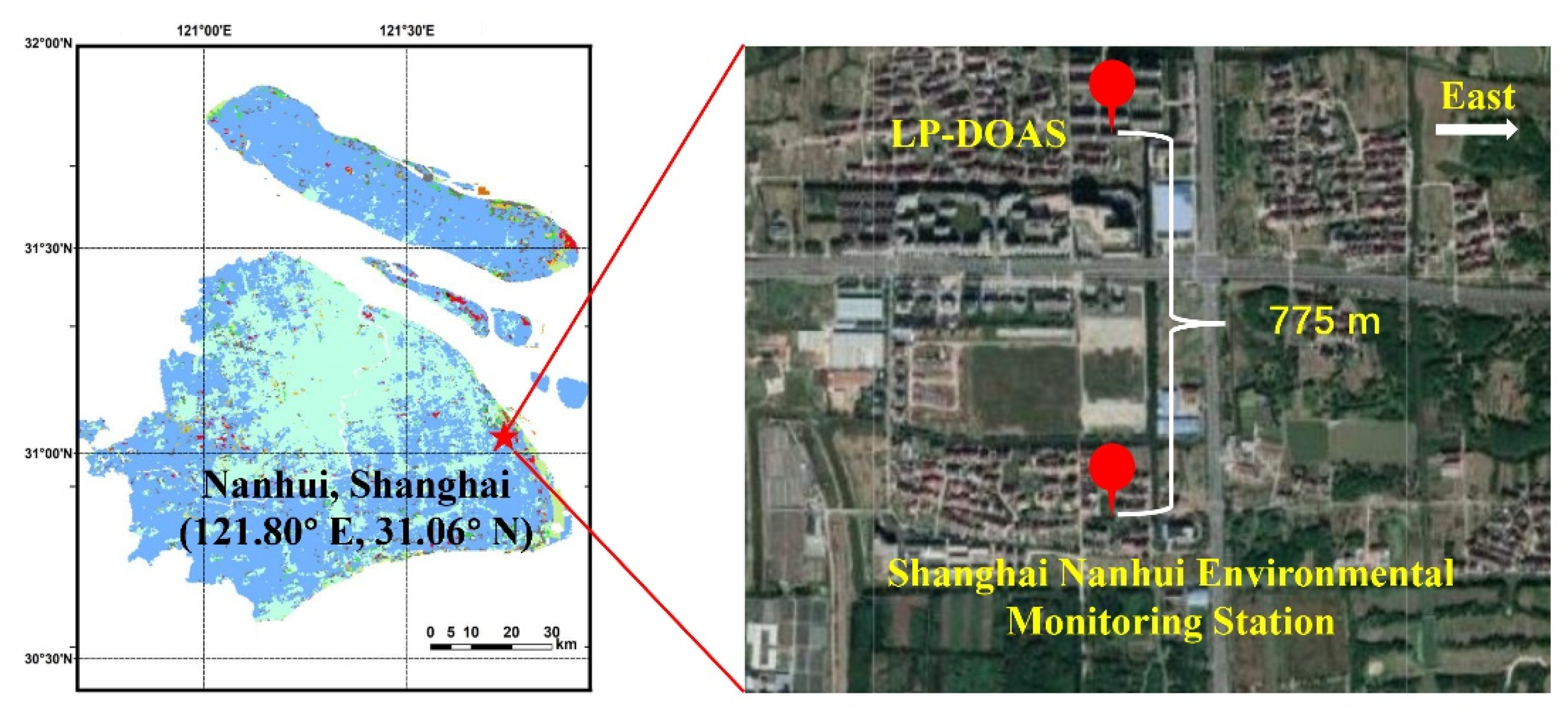
2.1. Measurement Site and Instrument Installation

A long-path DOAS (LP-DOAS) instrument was installed in Nanhui (121.80° E, 31.06° N), which is a suburb located east of Shanghai, China, about 10 km from the East China Sea coastline (Figure 1). Although several point sources of pollution such as the Laogang Chemical Industrial Park to the east and the Pudong International Airport to the north surround this site, heavy traffic emissions hardly occur. Overall, the area maintains lower levels of observed NOx, but nearly identical levels of O3 compared with the urban areas.
In order to monitor several different species synchronously, two collocated LP-DOAS systems were arranged for ultraviolet and visible wavelength ranges. Each LP-DOAS system consisted of the light source (150 W Xenon lamp for ultraviolet, light-emitting diode lamp for visible light), a light-emitting/receiving system with the telescope diameter of 210 mm, a spectrometer with a photodiode array detector (1024 pixels), and a computer as the controller. The instrument was mounted on the sixth floor of a residential building about 19 m above the ground. The retroreflector shared by the two systems was installed on the roof of the Shanghai Nanhui Environmental Monitoring Station, 775 m away from the observation site. The collimating beam emitted by the light source was reflected by the retroreflector after a certain distance transmission and finally collected by the receiving port. Afterwards, the light signals processed by the spectrometer were converted into electrical signals and recorded on the computer. In addition, the dark current and noise were removed during the measurement process by blocking the light emitted by the lamp and alternately collecting the background spectrum. The temporal resolution of spectral acquisition was six minutes.

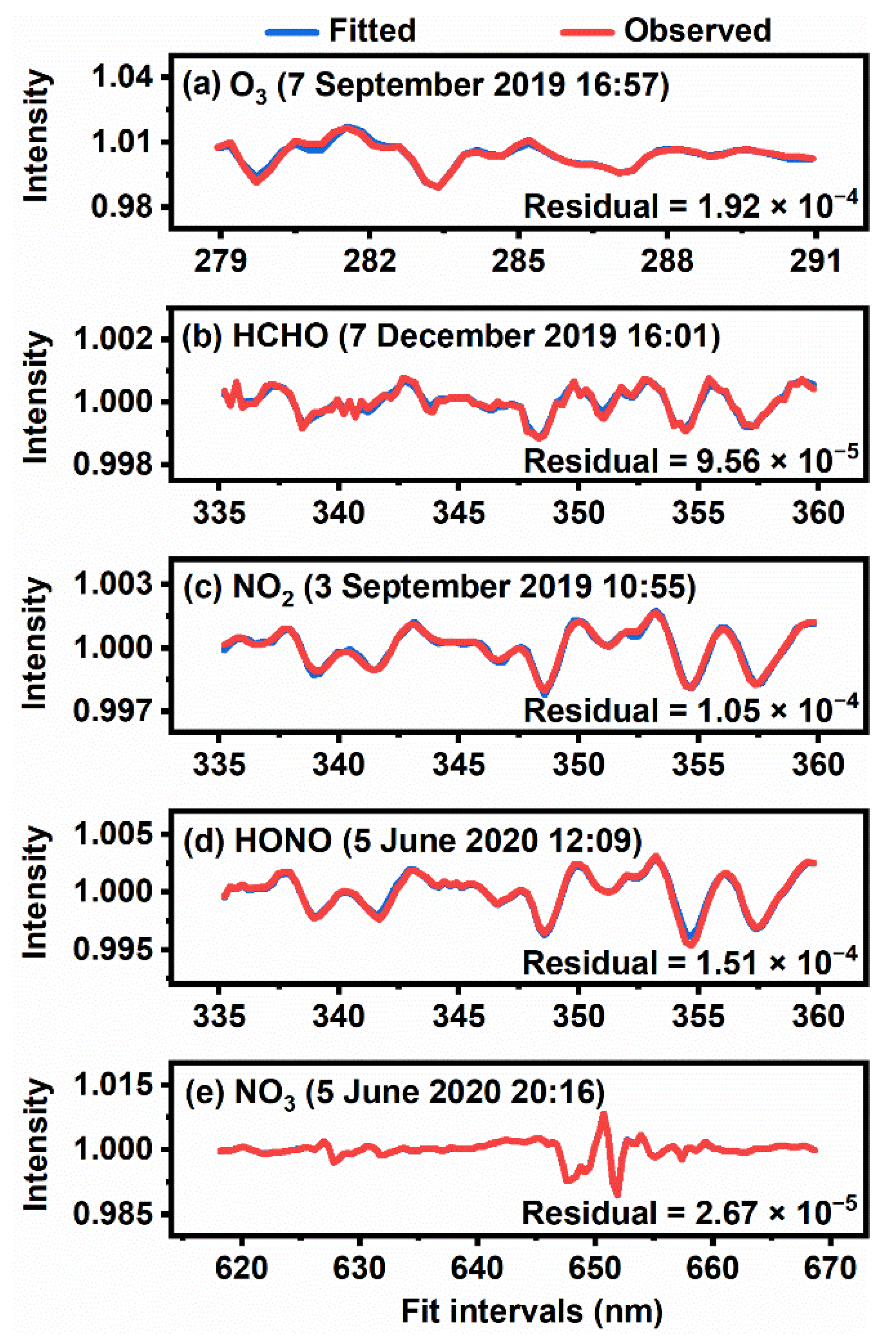
2.2. Spectral Analysis

DOAS is based on the Beer–Lambert law, which describes the relationship between the intensity of light absorption and the concentration of the light-absorbing substance of a certain wavelength. According to various differential absorption characteristics, the concentrations of O3, HCHO, NO2, and HONO in the atmosphere were retrieved through the observed ultraviolet spectra [18], while the concentration of NO3 was retrieved by visible spectra [19].
The spectral retrieval was mainly performed using DOASIS software developed by the Institute of Environmental Physics at Heidelberg University. For this study, the spectral analysis settings and detection limits of O3, HCHO, NO2, HONO, and NO3 retrieval are shown in Table S1. The high-resolution absorption cross-sections of NO2 [20], HCHO [21], SO2 [22], HONO [23], O3 [24], H2O (from the HITRAN database), and solar spectra were included in the fitting process. The theoretical detection limits are 2.0 ppbv for O3, 0.1 ppbv for HCHO and HONO, 1 ppbv for NO2, and 4 pptv for NO3.
Figure 2 presents typical DOAS spectral fitting results for O3, HCHO, NO2, HONO, and NO3. Moreover, the spectral retrieval results with residuals higher than 4 × 10⁻⁴ for HCHO, NO2, HONO, and NO3, and higher than 2 × 10⁻³ for O3 were filtered out. More than 90% of the results passed the filter, indicating the good performance of the DOAS spectral fitting. Additionally, intercomparison of O3 and NO2 measured by DOAS and in- situ instruments at the Shanghai Nanhui Environmental Monitoring Station verified the reliability of the DOAS measurements fitting as well (R2 > 0.9 for both) (Figure S1). The spectral fitting results within 1 h intervals were averaged for the following discussion.

2.3. Auxiliary Data

The time series of nitric oxide (NO) was obtained from the Shanghai Nanhui Environmental Monitoring Station, of which the temporal resolution was 1 h. All of the meteorological parameters used in this study, including temperature, relative humidity, wind, surface radiation, and boundary layer height, were obtained from the ERA5 data set of the European Centre for Medium-Range Weather Forecasts.

3. Results and Discussion

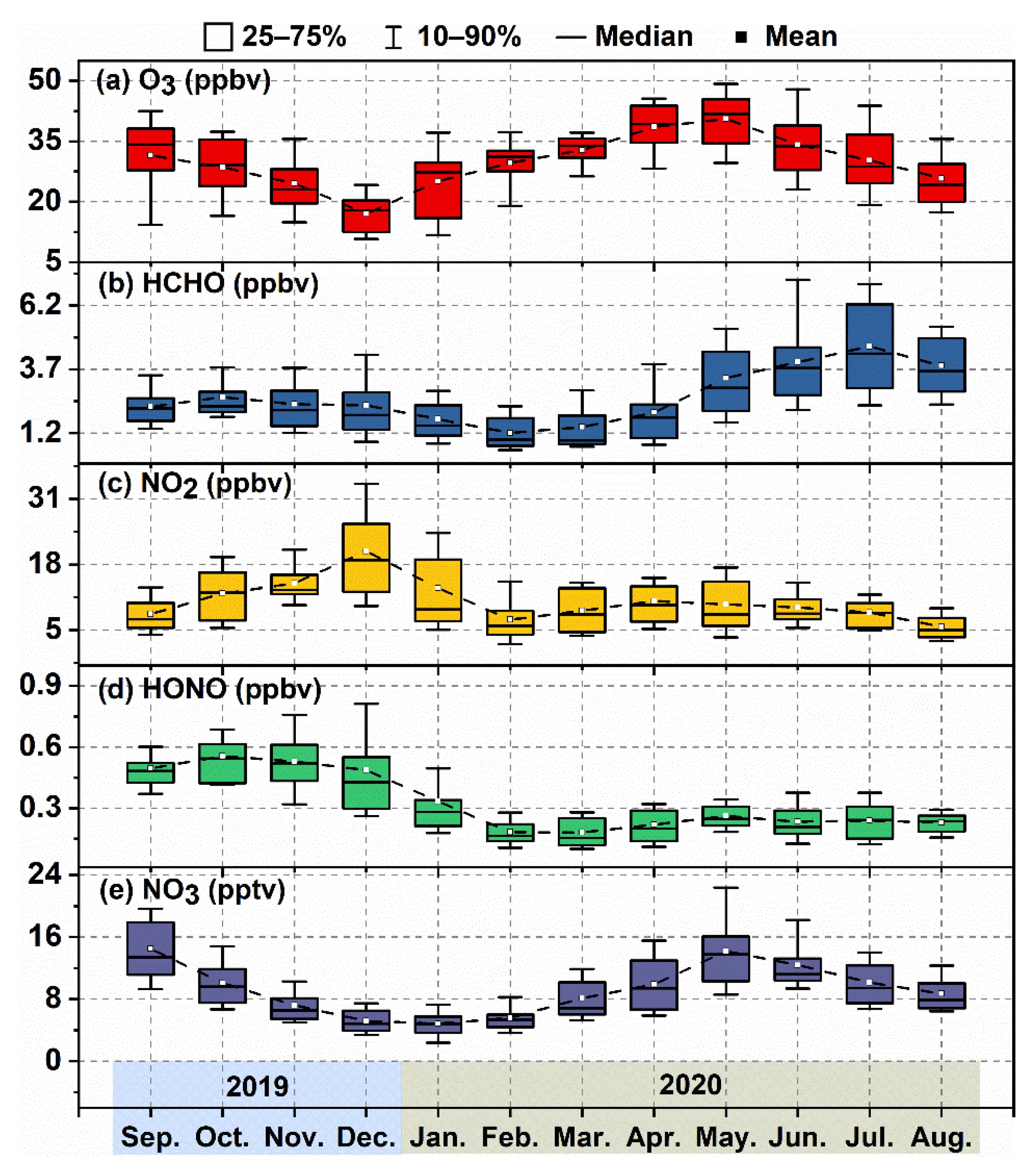
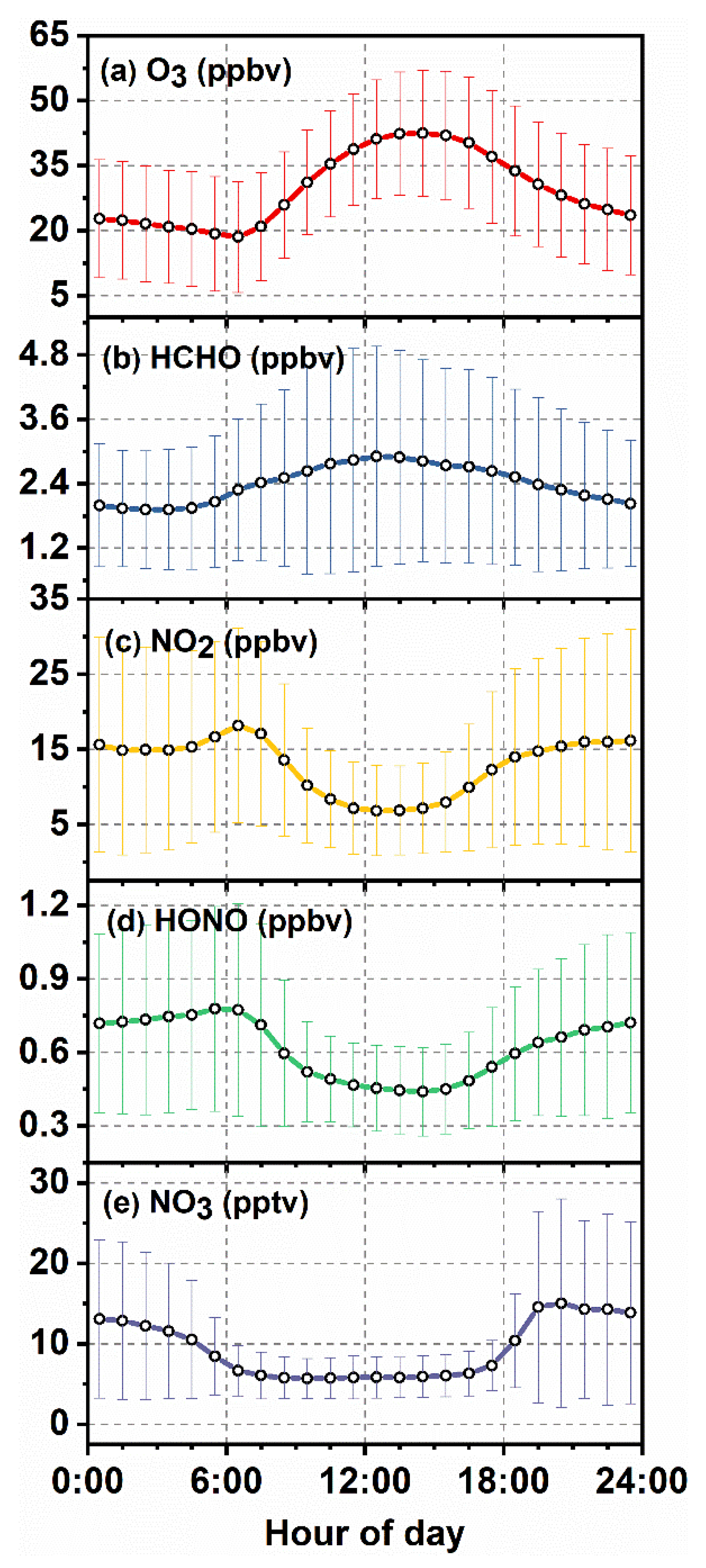
3.1. Overview of Observation

The monthly box charts of the daily means for O3, HCHO, NO2, HONO and NO3 measured by LP-DOAS from September 2019 to August 2020 are shown in Figure 3. The annual means of O3, HCHO, NO2, HONO, and NO3 were 34.33 ppbv, 2.41 ppbv, 12.77 ppbv, 0.61 ppbv and 9.34 pptv, respectively. Overall, the trend of monthly O3 averages presented a single peak during the year with a maximum of 40.56 ppbv and a minimum value of 17.00 ppbv in May 2020 and December 2019, respectively. This was a prominent reduction compared with 2014 to 2018 [25], indicating the remarkable delayed benefits of the continuous Clean Air Action Plan in China. It has been reported that O3 concentrations increased sharply in megacities with the implementation of the Clean Air Action Plan in 2013, but decreased after about three or four years later [26,27,28]. In addition, the Meiyu period in June and July of 2020 caused lower surface O3 concentrations, so it was not surprising that the O3 peaked in May 2020. Nevertheless, many higher O3 pollution episodes still occurred in summer even though the means were reduced, as displayed by the short lines of the 90th percentile in the box chart (Figure 3a).
Likewise, the variations in the mean HCHO concentrations revealed a single-peak trend throughout the year, with a maximum of 4.60 ppbv in July 2020 and a minimum of 1.20 ppbv in February 2020. The concentration of HCHO was comparable to the observation in summer 2018 in Shanghai reported by Guo et al. (2021) [29]. Compared to O3 and HCHO, NO2 and HONO depicted an opposite variation, the overall levels of both in 2019 were significantly higher than those in 2020. After December 2019, both dropped rapidly in January and February 2020, exhibiting a greater decline relative to the values in previous years [30,31]. This phenomenon is due to the COVID-19 lockdown in early 2020, which led to the reductions in anthropogenic activities and hence the pollutant emissions [32].
During the one-year observation period, there was a high concentration of NO3 radicals in the atmosphere in spring 2020, but a low concentration in winter 2019, depicting a trend similar to that of O3. Given that O3 and NO2 are the precursors of NO3 in the atmosphere and that the monthly variation in NO3 synchronized with O3, this indicated that the production of NO3 was regulated more by O3 than by NO2 at the observation site.
The diurnal variations in hourly O3, HCHO, NO2, HONO, and NO3 over the year were averaged as shown in Figure 4. O3 and HCHO manifested coincident diurnal single-peak trends with maximums of 42.35 and 2.91 ppbv at 14:00 and 12:00, respectively. The marked generation during the daytime implied that these species maintained rich secondary sources. The stage during which O3 levels declined before 06:00 was due to the titration effect caused by the increasing NO during rush hour when the generation of O3 was comparatively weak [33]. On average, O3 varied by 23.95 ppbv over a day, i.e., more than 100% of the daily minimum, while the variation in HCHO concentrations was 0.99 ppbv, i.e., approximately 50% of the daily minimum.
In contrast, the diurnal variations in NO2 and HONO exhibited single-valley trends with minimums of 6.84 and 0.44 ppbv at 12:00 and 14:00, respectively. Vehicle emissions contributed to the anthropogenic primary sources during the morning rush hour, which led to a slight increase in the concentrations of these species. With respect to NO3, the extreme photolysis during the daytime brought about a sustained minimal atmospheric concentration. After sunset, the NO3 concentration increased rapidly to its maximum level at 20:00. The average nighttime NO3 concentration reached 15 pptv, which was slightly lower than that observed in Shanghai in 2011 [34]. This phenomenon may be attributed to the current decrease in the precursors NO2 and O3.

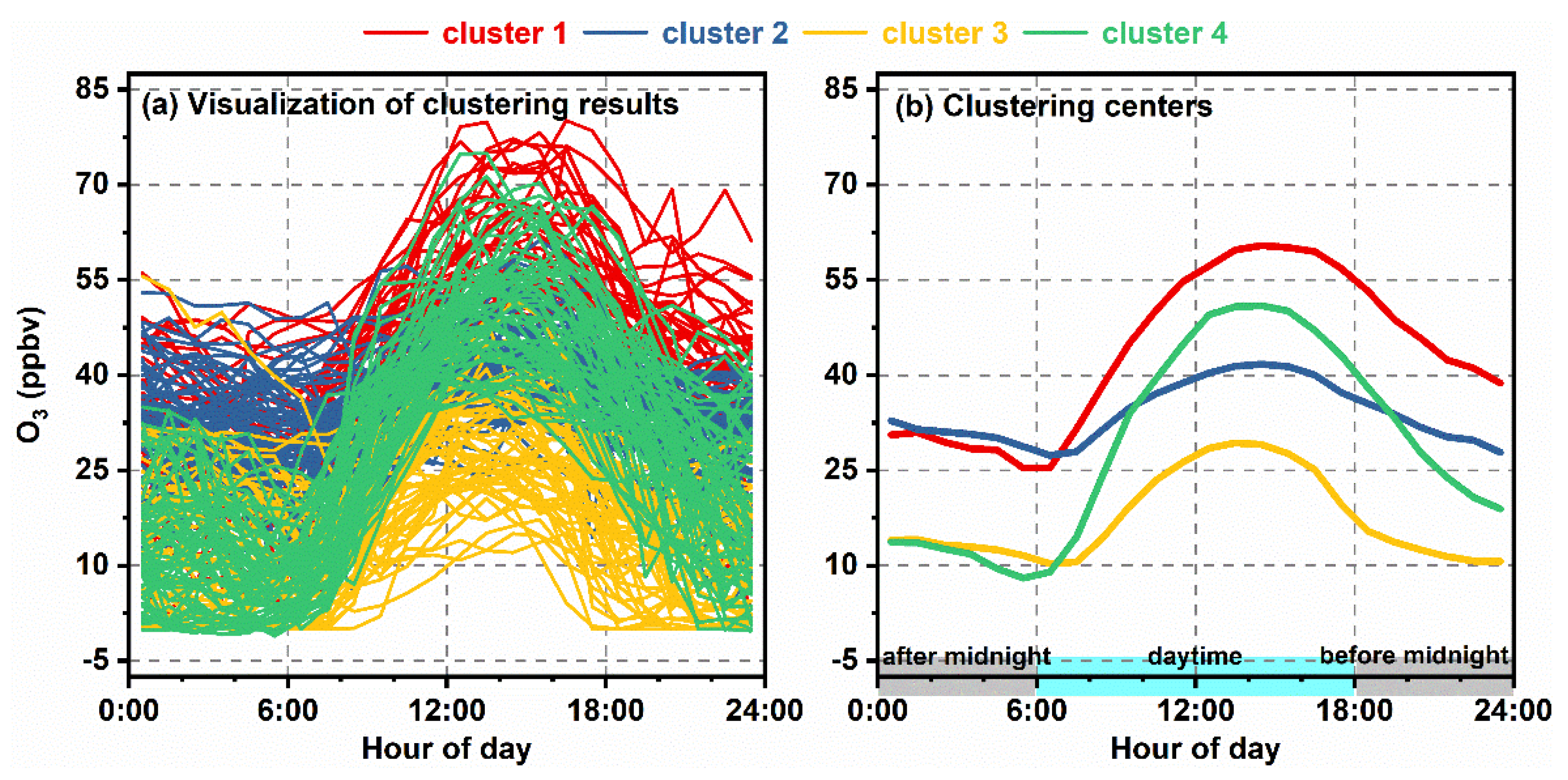
3.2. Clustering of O3 Diurnal Patterns

Admittedly, averaging over a time scale is a vital and traditional means to assess the temporal characteristics of pollutants. However, as discussed above, higher O3 levels at this observation site were found not only in summer, but also in spring and autumn. Seasonal categories could not integrally reflect the features of higher O3 conditions. In response, we aimed to discard the time limit and classify the O3 pollution based only on the characteristics of the daily O3 variation. Accordingly, K-means clustering methodology was used to identify groups of O3 pollution according to diurnal patterns, which enabled data objects to be assigned to the same cluster in accordance with common features [35]. Simultaneously, each cluster maintained distinct characteristics. Clustering analysis has been applied in atmospheric pollution for many years, especially using backward trajectory clustering [36].
Here, we defined the number of clustering units as four. Detailed information including determination of the optimal cluster number, the process of clustering, and evaluation of the clustering result, can be found in the Supplementary Materials. Visualization of the clustering results is displayed in Figure 5a. The monthly distribution of all the clusters were shown in Figure S6. Clusters 1 and 4 appeared more in autumn, spring and summer, i.e., the O3 pollution season in Shanghai. Additionally, cluster 3 appeared more in autumn and winter, whereas the distribution of cluster 2 was dispersed. The final four clustering centers shown in Figure 5b were used for the subsequent discussion. Additionally, the nighttime was divided into two parts, i.e., before (18:00–24:00) and after (00:00–06:00) midnight.
The O3 for cluster 1 retained a higher level after midnight and a higher production during the daytime. At the end of the daily cycle, daily accumulation was observed instead of backtracking to the original level. Similarly, cluster 2 was characterized by a higher nighttime background; however, its daytime generation was weak. In addition, the O3 concentration returned to the original level over a one-day period. Regarding cluster 3, the period after midnight revealed a relatively lower O3 concentration compared to clusters 1 and 2. After sunrise, the daytime increase was small, and the concentration just before midnight was equal to the daily minimum, which paralleled cluster 2. Cluster 4 reflected a lower level after midnight, but a considerable increase during the daytime, whereas before midnight, it dropped rapidly and eventually presented an increase of about 10 ppbv over a one-day period.
After identification of the four O3 diurnal pattern clusters, in order to explore the drivers of the O3 variations for the three different periods, relevant atmospheric components and meteorological factors for each cluster were averaged accordingly as illustrated in Figure 6. Furthermore, Table 1 briefly summarizes the information from Figure 6 for the four clusters in the different periods.
As shown in Figure 6a, the period after midnight produced an O3 gap of about 20 ppbv between clusters 1 and 2 and clusters 3 and 4. There was almost no O3 generation chemically at night, during which the response of the meteorological factors to the O3 concentration between clusters 1 and 2 and clusters 3 and 4 was indistinct, as shown in Figure 6. Therefore, the gap was considered to be the outcome of a depletion effect on the process of nocturnal atmospheric chemistry. Clusters 3 and 4 retained higher NO levels compared to clusters 1 and 2, as denoted in Figure 6e. Ambient NO reacted violently with O3 and was capable of accelerating the O3 consumption [37]. Therefore, NO was regarded as the driver of the O3 gap in this period.
During the daytime, the photochemical generation of O3 suggested a prominent difference between clusters 1 and 4 and clusters 2 and 3. Intense photochemical reactions (clusters 1 and 4) were detected accompanied by higher temperature, lower relative humidity, lower wind speed, and higher radiation, which accorded with the basic understanding of the photochemical reactions and has also been verified in previous studies [38,39]. With respect to precursors of photochemistry, the dominant roles of HCHO and NO2 in the generation of O3 cannot be neglected since it was confirmed that HCHO and NO2 are able to characterize the respective levels of VOCs and NOx in the atmosphere [40]. However, they displayed completely different behavior toward O3 variation (Figure 6g,h): HCHO was apparently higher for clusters 1 and 4 associated with evident O3 production, while NO2 was difficult to distinguish among them. This implied that the photochemical generation of O3 was basically dominated by VOCs rather than NOx in Shanghai, which has also been reported in previous studies [41,42].
The dependences of O3 on HCHO, HCHO/NO2, and NOx were surveyed as depicted in Figure 7. O3 concentration was found to correlate with HCHO for all clusters except for the low O3 cluster 3. Moreover, O3 correlated with HCHO/NO2, but negatively correlated with NOx for all clusters. For cluster 3, a strong negative correlation with NOx resulted in the good correlation with HCHO/NO2 in the case that the correlation with HCHO was poor. This provided important information for O3 control strategies.
Compared to the time after midnight, a more significant decline in surface O3 was revealed before midnight. This period indicated the diverse terminuses of the four clusters over the daily cycle. The O3 concentration for clusters 1 and 4 exhibited a certain accumulation, while clusters 2 and 3 regressed to the level of the daily minimum. Lower boundary layer heights were discovered for clusters 1 and 4 (Figure 6f), which directly hindered O3 diffusion and further led to the slow decline in ambient O3. Therefore, the boundary layer height seemed to be the driver of the O3 decline before midnight.

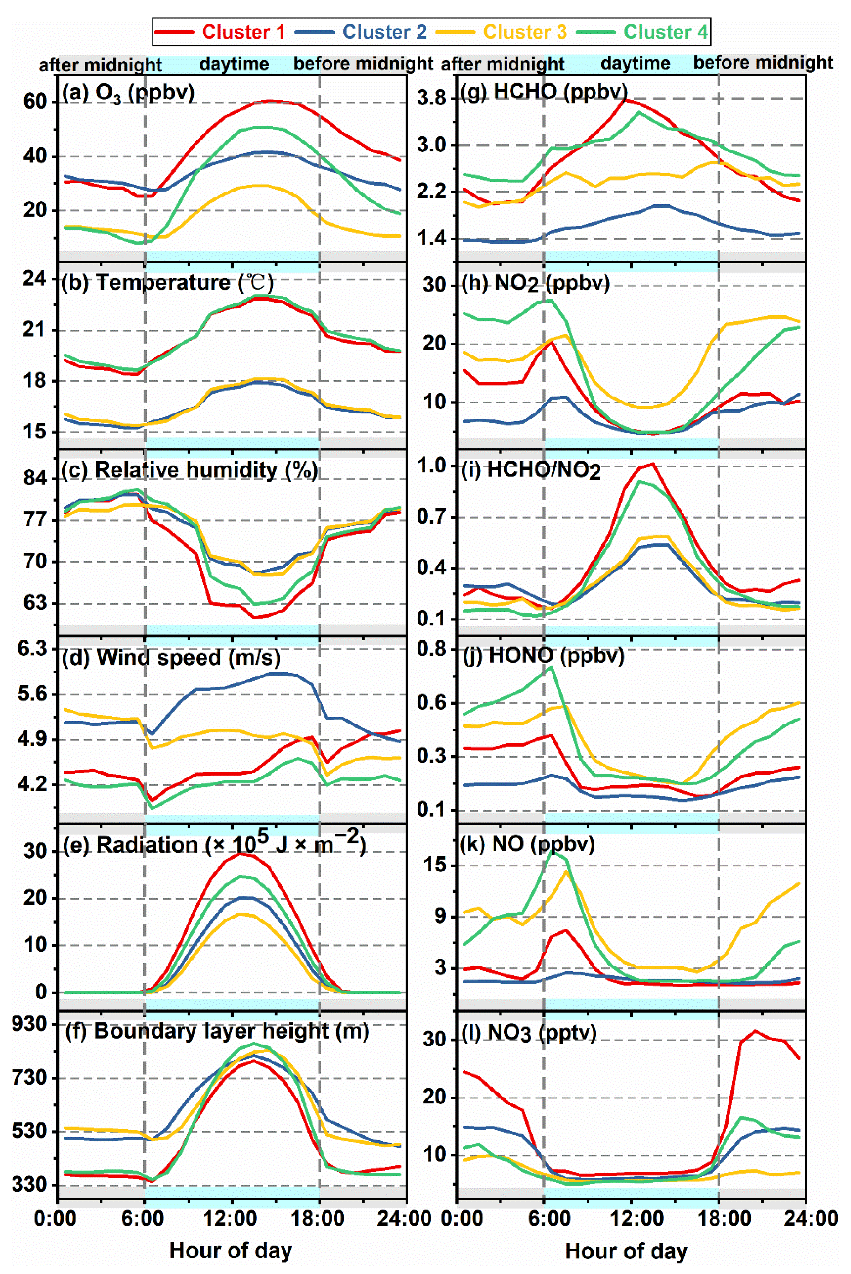
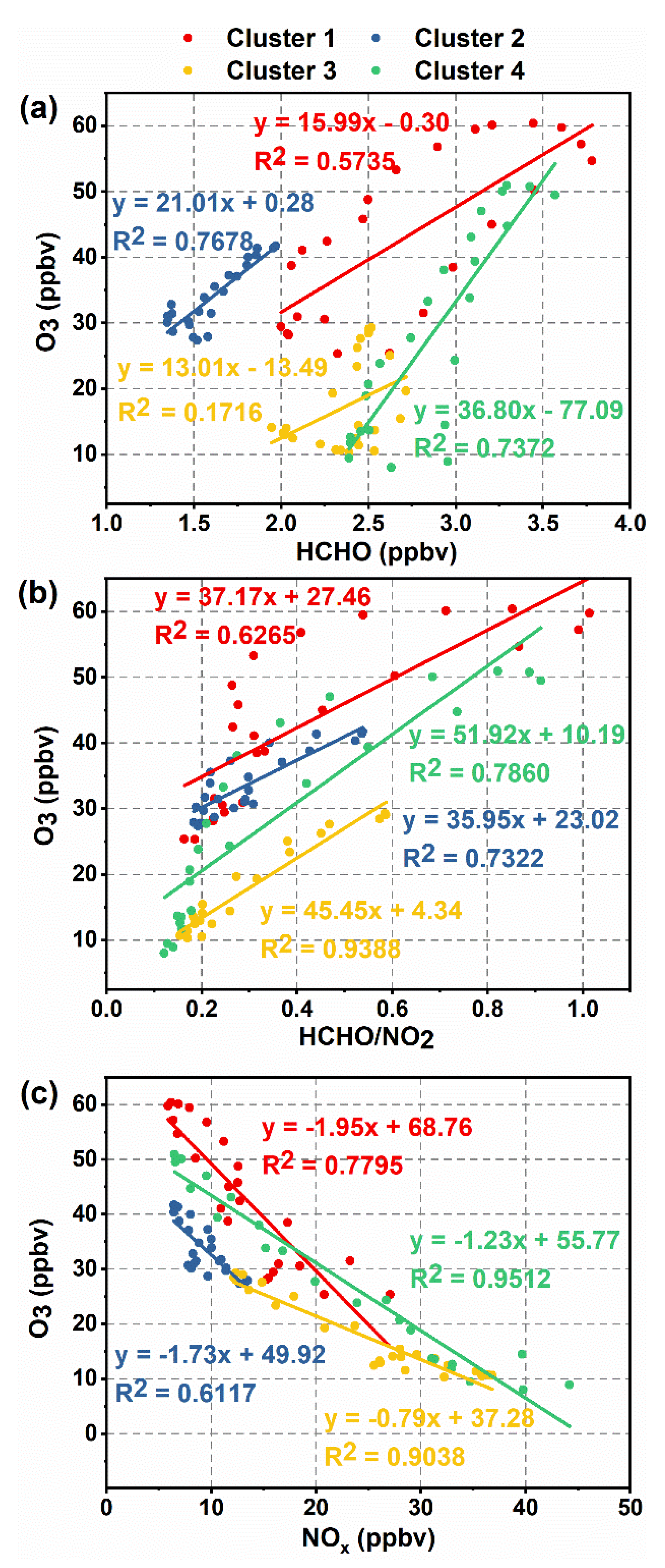
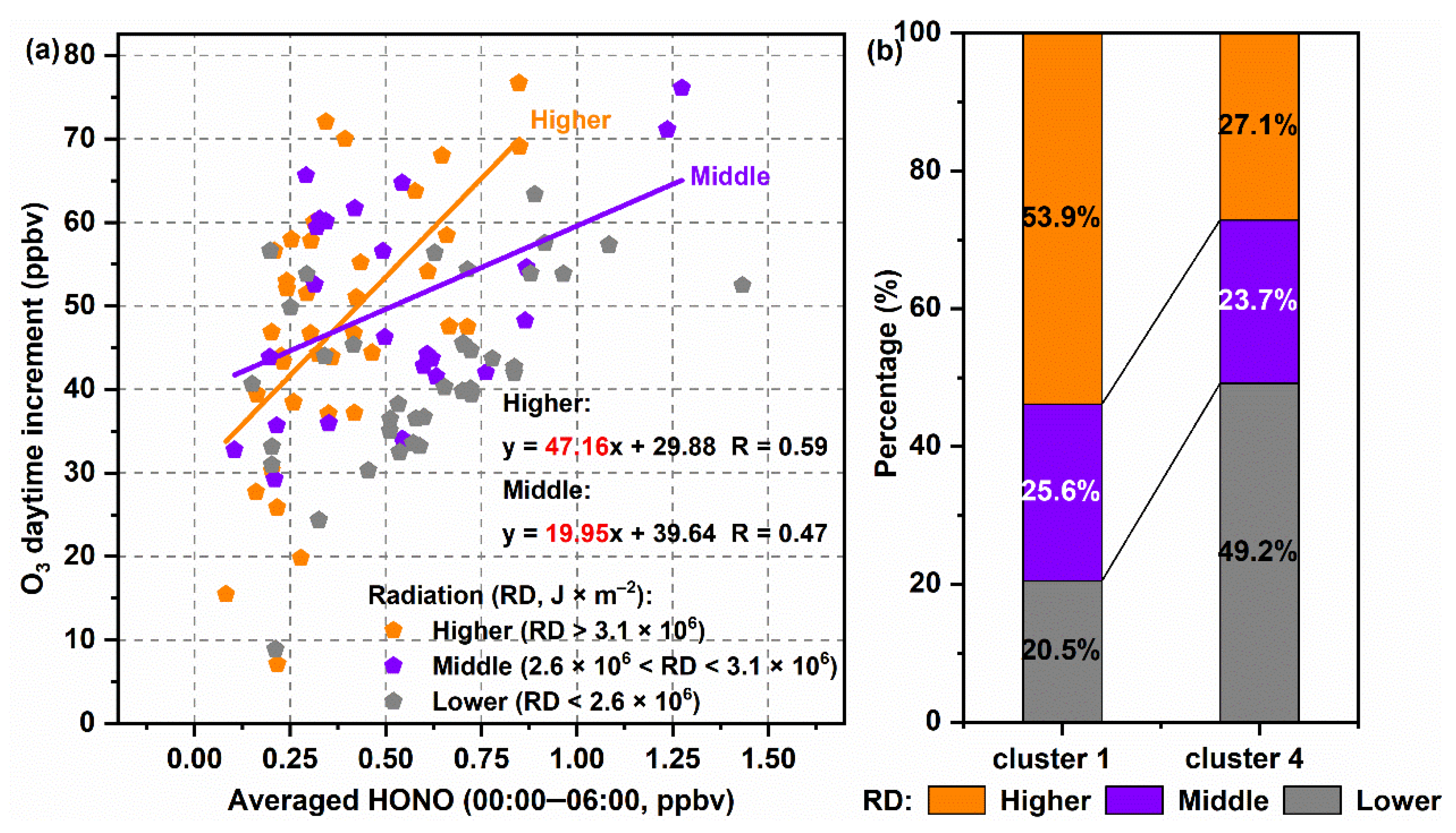
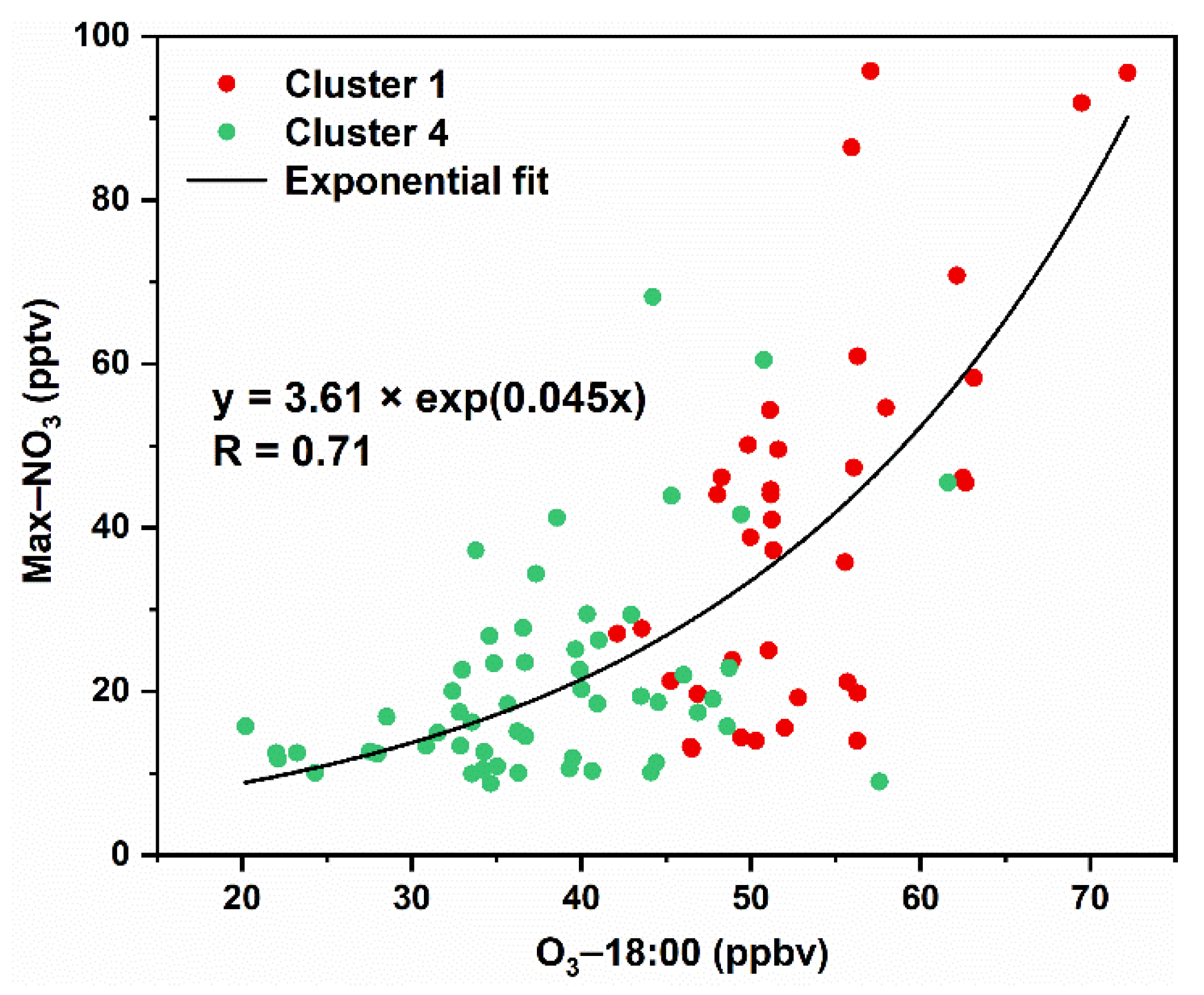
3.3. Interactions of Day- and Nighttime Atmospheric Components

In this section, we discuss the interactions among the three periods by taking the daytime period as the object. We investigated the impact of the period after midnight on the daytime as well as how it affected the period before midnight. Since the daytime was characterized by intense photochemical generation of O3, clusters 1 and 4 were suitably selected for the subsequent discussion.
The HONO levels of clusters 1 and 4 showed disparity after midnight (Figure 6j). After sunrise, the atmospheric HONO decreased rapidly because of the escalation of photolysis. The higher HONO level for cluster 4 resulted in a more prominent photochemistry as denoted by the more elevated O3 during the daytime in Figure 6a. The photolysis of HONO is an important source of OH radicals in the atmosphere [43,44]. HONO is able to significantly enhance the oxidation capacity of the atmosphere and further promote the photochemical generation of O3 [45,46].
The radiation for cluster 4 was found to be lower than that for cluster 1 during the daytime (Figure 6e); meanwhile, the O3 increase in cluster 4 was larger than that in cluster 1. We accordingly explored the influence of the radiation on HONO-O3 levels, as illustrated in Figure 8. When the radiation was higher, the daytime O3 increment showed the most sensitive reaction to the variation in averaged HONO after midnight, with a slope of 47.16. As radiation dropped to the middle level, the sensitivity was hence reduced, whereas the response between the O3 increment and the averaged HONO was unclear when radiation was lower than 2.6 × 10⁶ J·m−2. Figure 8b shows the proportions of radiation levels in clusters 1 and 4. It is obvious that cluster 1 was more occupied by higher radiation while lower radiation mainly covered cluster 4. Consequently, for cluster 4, it was not surprising to find the larger O3 increment even though the radiation was relatively low.
In terms of daytime O3 acting in the nighttime atmosphere, the NO3 level for clusters 1 and 4 was found to reflect a final gap of 16 pptv before midnight (Figure 6l), which could be attributed to the O3 difference after sunset. The larger remnant of O3 for cluster 1 in the daytime facilitated the generation of NO3 before midnight. NO3 is a crucial oxidant in the nocturnal atmosphere [19], which can trigger the conversion of a variety of VOCs, and NOx can also be removed from the atmosphere by further forming soluble nitrates after conversion into NO3 [47,48]. Therefore, the higher daytime O3 seemed to play a critical role in various nocturnal atmospheric chemical processes by generating more NO3.
Moreover, the relationship between the daily O3 concentration at 18:00 and the maximum NO3 before midnight was investigated (Figure 9). The O3 level at 18:00 was considered the endpoint of generation and loss during the daytime. Overall, max-NO3 exhibited an exponential growth with O3-18:00, suggesting that the increase tended to be faster gradually. Cluster 1 evidently experienced a steeper rise than cluster 4 owing to the larger persistent level of O3 in the daytime.
Furthermore, in order to explore O3 pollution associated with the meteorological conditions and the corresponding variability of the relative atmospheric components at a more detailed level, a case study of a high O3 pollution episode was carried out as shown in Supplementary Materials (Figure S7, Table S2). The in-depth analysis of the case study is also found to be consistent with the clustering characteristics.

4. Conclusions

The current study surveyed O3, HCHO, NO2, HONO and NO3 concentrations from September 2019 to August 2020 based on LP-DOAS measurements in Nanhui, Shanghai. Here, we classified O3 diurnal patterns into four clusters using the K-means clustering methodology, the differences among which were manifested in three periods: daytime and before and after midnight. The relevant atmospheric components and meteorological factors were examined purposefully.
The period after midnight showed an evident O3 gap between clusters 1 and 2 and clusters 3 and 4, which was driven by different ambient NO. During the daytime, the intense photochemistry was found to strongly depend on the meteorological conditions of higher temperature, lower humidity, lower wind speed and higher radiation. O3 correlated with HCHO/NO2, but negatively correlated with NOx for all clusters. The HCHO/NO2 ratio was an excellent indicator of the O3 levels rather than HCHO itself. Moreover, the lower boundary layer height before midnight seemed to hinder the diffusion of O3, which resulted in an accumulation at the end of the daily cycle. The interactions among the three periods of the diurnal pattern were analyzed for clusters 1 and 4. The daytime O3 levels showed a consensus with the HONO levels after midnight, during which time radiation conditionally played a role. In addition, the cumulative O3 in the daytime determined the level of NO3 production before midnight.
As the DOAS method can simultaneously detect multiple trace gases in the atmosphere, we determined that the relationship between active atmospheric components and O3 pollution can be reviewed from the perspective of diurnal interaction. Therefore, this paper provides novel inspiration for the future study and management of regional O3 pollution.

Supplementary Materials

The following supporting information can be downloaded at: https://0-www-mdpi-com.brum.beds.ac.uk/article/10.3390/atmos13020351/s1. Table S1. DOAS fit settings and detection limits for O3, NO2, HCHO, HONO and NO3; Table S2. A summary of the relevant atmospheric components for each day; Figure S1. Time series of the O3 and NO2 mixing ratios of the DOAS retrieval, and the linear fitting, mean bias and the standard deviation for the two observation methods; Figure S2. DBI values for the number of clusters from 1 to 10. Figure S3. The process of clustering in this study; Figure S4. Bar plots of the silhouette coefficient values for all the diurnal patterns; Figure S5. The SC values when the cluster number is defined range from 2 to 10; Figure S6. The monthly distribution of clustering result; Figure S7. Time series of O3, HCHO and NO2, HCHO/NO2 and NO, NO3 and HONO, temperature (T) and relative humidity (RH), wind speed (WS), boundary layer height (BLH) and radiation (R).

Author Contributions

X.W., S.W. and B.Z. designed and implemented the research, as well as prepared the manuscript; S.Z. and C.G. contributed to the DOAS measurements and spectral analysis; R.Z. and A.T. revised the manuscript. All authors have read and agreed to the published version of the manuscript.

Funding

This research was funded by the National Natural Science Foundation of China grant number 21976031, 42075097 and 22176037.

Institutional Review Board Statement

Not applicable.

Informed Consent Statement

Not applicable.

Data Availability Statement

Data are available for scientific purposes upon request to the corresponding authors.

Conflicts of Interest

The authors declare that they have no conflict of interest.

References

  1. Qiu, W.Y.; Li, S.L.; Liu, Y.H.; Lu, K.D. Petrochemical and industrial sources of volatile organic compounds analyzed via regional wind-driven network in Shanghai. Atmosphere 2019, 10, 760. [Google Scholar] [CrossRef] [Green Version]
  2. Zhang, J.; Li, D.; Bian, J.; Bai, Z. Deep stratospheric intrusion and Russian wildfire induce enhanced tropospheric ozone pollution over the northern Tibetan Plateau. Atmos. Res. 2021, 259, 105662. [Google Scholar] [CrossRef]
  3. Alejandro, S.; Valdes, H.; Zaror, C.A. Natural zeolite reactivity towards ozone: The role of acid surface sites. Adv. Oxid. Technol. J. 2011, 14, 182–189. [Google Scholar] [CrossRef]
  4. Schnell, J.L.; Prather, M.J.; Josse, B.; Naik, V.; Horowitz, L.W.; Zeng, G.; Shindell, D.T.; Faluvegi, G. Effect of climate change on surface ozone over North America, Europe, and East Asia. Geophys. Res. Lett. 2016, 43, 3509–3518. [Google Scholar] [CrossRef] [PubMed] [Green Version]
  5. Unger, N.; Zheng, Y.Q.; Yue, X.; Harper, K.L. Mitigation of ozone damage to the world’s land ecosystems by source sector. Nat. Clim. Chang. 2020, 10, 134–137. [Google Scholar] [CrossRef]
  6. Li, K.; Jacob, D.J.; Liao, H.; Shen, L.; Zhang, Q.; Bates, K.H. Anthropogenic drivers of 2013–2017 trends in summer surface ozone in China. Proc. Natl. Acad. Sci. USA 2019, 116, 422–427. [Google Scholar] [CrossRef] [Green Version]
  7. Wang, T.; Xue, L.; Brimblecombe, P.; Lam, Y.F.; Li, L.; Zhang, L. Ozone pollution in China: A review of concentrations, meteorological influences, chemical precursors, and effects. Sci. Total Environ. 2017, 575, 1582–1596. [Google Scholar] [CrossRef]
  8. Liu, P.F.; Song, H.Q.; Wang, T.H.; Wang, F.; Li, X.Y.; Miao, C.H.; Zhao, H.P. Effects of meteorological conditions and anthropogenic precursors on ground-level ozone concentrations in Chinese cities. Environ. Pollut. 2020, 262, 8. [Google Scholar] [CrossRef]
  9. Wang, N.; Lyu, X.P.; Deng, X.J.; Huang, X.; Jiang, F.; Ding, A.J. Aggravating O3 pollution due to NOx emission control in eastern China. Sci. Total Environ. 2019, 677, 732–744. [Google Scholar] [CrossRef] [PubMed]
  10. Chen, Z.Y.; Li, R.Y.; Chen, D.L.; Zhuang, Y.; Gao, B.B.; Yang, L.; Li, M.C. Understanding the causal influence of major meteorological factors on ground ozone concentrations across China. J. Clean. Prod. 2020, 242, 13. [Google Scholar] [CrossRef]
  11. Chen, Z.Y.; Zhuang, Y.; Xie, X.M.; Chen, D.L.; Cheng, N.L.; Yang, L.; Li, R.Y. Understanding long-term variations of meteorological influences on ground ozone concentrations in Beijing During 2006–2016. Environ. Pollut. 2019, 245, 29–37. [Google Scholar] [CrossRef] [PubMed]
  12. Shan, W.P.; Yin, Y.Q.; Zhang, J.D.; Ji, X.; Deng, X.Y. Surface ozone and meteorological condition in a single year at an urban site in central-eastern China. Environ. Monit. Assess. 2009, 151, 127–141. [Google Scholar] [CrossRef] [PubMed]
  13. Yan, J.J.; Wang, G.L.; Yang, P.C. Study on the Sensitivity of Summer Ozone Density to the Enhanced Aerosol Loading over the Tibetan Plateau. Atmosphere 2020, 11, 138. [Google Scholar] [CrossRef] [Green Version]
  14. Yu, D.; Tan, Z.; Lu, K.; Ma, X.; Li, X.; Chen, S.; Zhu, B.; Lin, L.; Li, Y.; Qiu, P.; et al. An explicit study of local ozone budget and NOx-VOCs sensitivity in Shenzhen China. Atmos. Environ. 2020, 224, 13. [Google Scholar] [CrossRef]
  15. Sun, L.Q.; Cheng, K.X.; Yang, H.D.; He, Q.S. An on-line monitoring technique for Trace Gases in Atmosphere Based on Differential optical absorption spectroscopy. In Proceedings of the 2nd Conference of the Optics-and-Photonics-Society-of-Singapore/International Conference on Optics in Precision Engineering and Nanotechnology (icOPEN), Singapore, 9–11 April 2013; Volume 8769. [Google Scholar]
  16. Allegrini, I.; Febo, A.; Giliberti, C.; Perrino, C. Intercomparison of DOAS and conventional analysers in the measurement of atmospheric pollutants in an urban background monitoring site of Rome. In Proceedings of the Conference on Remote Sensing of Vegetation and Water, and Standardization of Remote Sensing Methods, Munich, Germany, 18–19 June 1997; Volume 3107, pp. 64–73. [Google Scholar]
  17. Hoffman, S.; Sulkowski, W.; Krzyzanowski, K. The urban ozone monitoring by the DOAS technique application. J. Mol. Struct. 1995, 348, 187–189. [Google Scholar] [CrossRef]
  18. Zhu, J.; Wang, S.S.; Wang, H.L.; Jing, S.G.; Lou, S.R.; Saiz-Lopez, A.; Zhou, B. Observationally constrained modeling of atmospheric oxidation capacity and photochemical reactivity in Shanghai, China. Atmos. Chem. Phys. 2020, 20, 1217–1232. [Google Scholar] [CrossRef] [Green Version]
  19. Yan, Y.H.; Wang, S.S.; Zhu, J.; Guo, Y.L.; Tang, G.Q.; Liu, B.X.; An, X.X.; Wang, Y.S.; Zhou, B. Vertically increased NO3 radical in the nocturnal boundary layer. Sci. Total Environ. 2021, 763, 12. [Google Scholar] [CrossRef]
  20. Voigt, S.; Orphal, J.; Burrows, J.P. The temperature and pressure dependence of the absorption cross-sections of NO2 in the 250–800 nm region measured by Fourier-transform spectroscopy. J. Photochem. Photobiol. A-Chem. 2002, 149, 1–7. [Google Scholar] [CrossRef]
  21. Meller, R.; Moortgat, G.K. Temperature dependence of the absorption cross sections of formaldehyde between 223 and 323 K in the wavelength range 225–375 nm. J. Geophys. Res.-Atmos. 2000, 105, 7089–7101. [Google Scholar] [CrossRef]
  22. Hermans, C.; Vandaele, A.C.; Fally, S. Fourier transform measurements of SO2 absorption cross sections: I. Temperature dependence in the 24,000–29,000 cm−1 (345–420 nm) region. J. Quant. Spectrosc. Radiat. Transf. 2009, 110, 756–765. [Google Scholar] [CrossRef]
  23. Stutz, J.; Kim, E.S.; Platt, U.; Bruno, P.; Perrino, C.; Febo, A. UV-visible absorption cross sections of nitrous acid. J. Geophys. Res.-Atmos. 2000, 105, 14585–14592. [Google Scholar] [CrossRef]
  24. Voigt, S.; Orphal, J.; Bogumil, K.; Burrows, J.P. The temperature dependence (203–293 K) of the absorption cross sections of O3 in the 230–850 nm region measured by Fourier-transform spectroscopy. J. Photochem. Photobiol. A-Chem. 2001, 143, 1–9. [Google Scholar] [CrossRef]
  25. Wu, J.; Xiao, B. Study on near-surface ozone pollution in Shanghai urban area. Guangzhou Chem. Ind. 2020, 48, 112–116, 156. [Google Scholar]
  26. Xu, J.M.; Tie, X.X.; Gao, W.; Lin, Y.F.; Fu, Q.Y. Measurement and model analyses of the ozone variation during 2006 to 2015 and its response to emission change in megacity Shanghai, China. Atmos. Chem. Phys. 2019, 19, 9017–9035. [Google Scholar] [CrossRef] [Green Version]
  27. Tang, G.; Liu, Y.; Zhang, J.; Liu, B.; Li, Q.; Sun, J.; Wang, Y.; Xuan, Y.; Li, Y.; Pan, J.; et al. Bypassing the NOx titration trap in ozone pollution control in Beijing. Atmos. Res. 2021, 249, 105333. [Google Scholar] [CrossRef]
  28. Zhang, J.; Li, D.; Bian, J.; Xuan, Y.; Chen, H.; Bai, Z.; Wan, X.; Zheng, X.; Xia, X.; Lu, D. Long-term ozone variability in the vertical structure and integrated column over the North China Plain: Results based on ozonesonde and Dobson measurements during 2001–2019. Environ. Res. Lett. 2021, 16, 074053. [Google Scholar] [CrossRef]
  29. Guo, Y.L.; Wang, S.S.; Zhu, J.; Zhang, R.F.; Gao, S.; Saiz-Lopez, A.; Zhou, B. Atmospheric formaldehyde, glyoxal and their relations to ozone pollution under low- and high-NOx regimes in summertime Shanghai, China. Atmos. Res. 2021, 258, 10. [Google Scholar] [CrossRef]
  30. Chen, Y.Y.; Bai, Y.; Liu, H.T.; Alatalo, J.M.; Jiang, B. Temporal variations in ambient air quality indicators in Shanghai municipality, China. Sci. Rep. 2020, 10, 11. [Google Scholar] [CrossRef]
  31. Li, D.D.; Xue, L.K.; Wen, L.; Wang, X.F.; Chen, T.S.; Mellouki, A.; Chen, J.M.; Wang, W.X. Characteristics and sources of nitrous acid in an urban atmosphere of northern China: Results from 1-yr continuous observations. Atmos. Environ. 2018, 182, 296–306. [Google Scholar] [CrossRef] [Green Version]
  32. Tanvir, A.; Javed, Z.; Jian, Z.; Zhang, S.B.; Bilal, M.; Xue, R.B.; Wang, S.S.; Bin, Z. Ground-Based MAX-DOAS Observations of Tropospheric NO2 and HCHO During COVID-19 Lockdown and Spring Festival Over Shanghai, China. Remote Sens. 2021, 13, 488. [Google Scholar] [CrossRef]
  33. Fu, Z.Q.; Dai, C.H.; Wang, Z.W.; Guo, J.; Qin, P.F.; Zhang, X.S. Sensitivity analysis of atmospheric ozone formation to its precursors in summer of Changsha. Environ. Chem. 2019, 38, 531–538. [Google Scholar]
  34. Wang, S.S.; Shi, C.Z.; Zhou, B.; Zhao, H.; Wang, Z.R.; Yang, S.N.; Chen, L.M. Observation of NO3 radicals over Shanghai, China. Atmos. Environ. 2013, 70, 401–409. [Google Scholar] [CrossRef]
  35. Govender, P.; Sivakumar, V. Application of k-means and hierarchical clustering techniques for analysis of air pollution: A review (1980–2019). Atmos. Pollut. Res. 2020, 11, 40–56. [Google Scholar] [CrossRef]
  36. Darby, L.S. Cluster analysis of surface winds in Houston, Texas, and the impact of wind patterns on ozone. J. Appl. Meteorol. 2005, 44, 1788–1806. [Google Scholar] [CrossRef]
  37. Awang, N.R.; Ramli, N.A.; Yahaya, A.S.; Elbayoumi, M. High Nighttime Ground-Level Ozone Concentrations in Kemaman: NO and NO2 Concentrations Attributions. Aerosol Air Qual. Res. 2015, 15, 1357–1366. [Google Scholar] [CrossRef]
  38. An, J.L.; Hang, Y.X.; Zhu, B.; Wang, D.D. Observational study of ozone concentrations in northern suburb of Nanjing. Ecol. Environ. Sci. 2010, 19, 1383–1386. [Google Scholar]
  39. Li, M.Y.; Yu, S.C.; Chen, X.; Li, Z.; Zhang, Y.B.; Wang, L.Q.; Liu, W.P.; Li, P.F.; Lichtfouse, E.; Rosenfeld, D.; et al. Large scale control of surface ozone by relative humidity observed during warm seasons in China. Environ. Chem. Lett. 2021, 19, 3981–3989. [Google Scholar] [CrossRef]
  40. Hong, Q.Q.; Liu, C.; Hu, Q.H.; Zhang, Y.L.; Xing, C.Z.; Su, W.J.; Ji, X.G.; Xiao, S.X. Evaluating the feasibility of formaldehyde derived from hyperspectral remote sensing as a proxy for volatile organic compounds. Atmos. Res. 2021, 264, 12. [Google Scholar] [CrossRef]
  41. Lin, H.T.; Wang, M.; Duan, Y.S.; Fu, Q.Y.; Ji, W.H.; Cui, H.X.; Jin, D.; Lin, Y.F.; Hu, K. O3 sensitivity and contributions of different NMHC sources in O3 formation at urban and suburban sites in Shanghai. Atmosphere 2020, 11, 295. [Google Scholar] [CrossRef] [Green Version]
  42. Yang, L.F.; Yuan, Z.B.; Luo, H.H.; Wang, Y.R.; Xu, Y.Q.; Duan, Y.S.; Fu, Q.Y. Identification of long-term evolution of ozone sensitivity to precursors based on two-dimensional mutual verification. Sci. Total Environ. 2021, 760, 9. [Google Scholar] [CrossRef]
  43. Alicke, B.; Geyer, A.; Hofzumahaus, A.; Holland, F.; Konrad, S.; Patz, H.W.; Schafer, J.; Stutz, J.; Volz-Thomas, A.; Platt, U. OH formation by HONO photolysis during the BERLIOZ experiment. J. Geophys. Res.-Atmos. 2003, 108, 17. [Google Scholar] [CrossRef] [Green Version]
  44. Harris, G.W.; Carter, W.P.L.; Winer, A.M.; Pitts, J.N.; Platt, U.; Perner, D. Observations of nitrous-acid in the Los-Angeles atmosphere and implications for predictions of ozone precursor relationships. Environ. Sci. Technol. 1982, 16, 414–419. [Google Scholar] [CrossRef] [PubMed]
  45. Fu, X.; Wang, T.; Zhang, L.; Li, Q.Y.; Wang, Z.; Xia, M.; Yun, H.; Wang, W.H.; Yu, C.; Yue, D.L.; et al. The significant contribution of HONO to secondary pollutants during a severe winter pollution event in southern China. Atmos. Chem. Phys. 2019, 19, 1–14. [Google Scholar] [CrossRef] [Green Version]
  46. Jia, C.H.; Tong, S.R.; Zhang, W.Q.; Zhang, X.R.; Li, W.R.; Wang, Z.; Wang, L.L.; Liu, Z.R.; Hu, B.; Zhao, P.S.; et al. Pollution characteristics and potential sources of nitrous acid (HONO) in early autumn 2018 of Beijing. Sci. Total Environ. 2020, 735, 11. [Google Scholar] [CrossRef] [PubMed]
  47. Brown, S.S.; Stutz, J. Nighttime radical observations and chemistry. Chem. Soc. Rev. 2012, 41, 6405–6447. [Google Scholar] [CrossRef]
  48. Pye, H.O.T.; Chan, A.W.H.; Barkley, M.P.; Seinfeld, J.H. Global modeling of organic aerosol: The importance of reactive nitrogen (NOx and NO3). Atmos. Chem. Phys. 2010, 10, 11261–11276. [Google Scholar] [CrossRef] [Green Version]
Figure 1. The topographic locations of the LP-DOAS instrument and Shanghai Nanhui Environmental Monitoring Station (© Google Earth).
Atmosphere 13 00351 g001
Figure 2. Examples of typical DOAS spectral fitting results for O3 (a), HCHO (b), NO2 (c), HONO (d), and NO3 (e) including the observed and fitted result.
Atmosphere 13 00351 g002
Figure 3. The monthly box charts of O3 (a), HCHO (b), NO2 (c), HONO (d), and NO3 (e) from September 2019 to August 2020 in Nanhui, Shanghai. The monthly means are connected by black dotted lines.
Atmosphere 13 00351 g003
Figure 4. The mean diurnal variations in O3 (a), HCHO (b), NO2 (c), HONO (d), and NO3 (e) from September 2019 to August 2020 in Nanhui, Shanghai. (The error bars indicate the standard deviations).
Atmosphere 13 00351 g004
Figure 5. Visualization of the clustering results (a) and the final four clustering centers of the O3 diurnal pattern (b).
Atmosphere 13 00351 g005
Figure 6. Diurnal variations in O3 (a) and the meteorological factors (temperature (b), relative humidity (c), wind speed (d), radiation (e), and boundary layer height (f)) as well as the relevant atmospheric components (HCHO (g), NO2 (h), HCHO/NO2 (i), HONO (j), NO (k), and NO3 (l)).
Atmosphere 13 00351 g006
Figure 7. The O3 concentrations and corresponding HCHO concentrations (a), HCHO/NO2 ratios (b), and NOx concentrations (c) for the four clusters. Colored lines represent the linear fit for each cluster.
Atmosphere 13 00351 g007
Figure 8. The dependence of the O3 increment in clusters 1 and 4 on the HONO concentration under different radiation conditions (a) and the radiation distributions of clusters 1 and cluster 4 (b).
Atmosphere 13 00351 g008
Figure 9. The daily O3 concentration at 18:00 and the maximum concentration of NO3 between 18:00 and 23:00 in clusters 1 and 4.
Atmosphere 13 00351 g009
Table 1. A summary of the information visualized in Figure 6 for the four clusters in different periods.
PeriodSpeciesCluster 1Cluster 2Cluster 3Cluster 4
After midnightO3 levelhigherhigherlowerlower
NO titrationweakweakintenseintense
HONO levellower////higher
DaytimeO3 increaselower////higher
Photochemical levelintenseweakweakintense
Meteorological factors for photochemical reaction (T, RH, WS, R)favorableadverseadversefavorable
Before midnightO3-18:00higher////lower
max-NO3higher////lower
BLHlowerhigherhigherlower
O3 accumulationyes//yes
T, RH, WS, R, and BLH represent temperature, relative humidity, wind speed, radiation, and boundary layer height, respectively. “/” represents a null value, while “//” in clusters 2 and 3 indicates that it is not discussed in this study.
Publisher’s Note: MDPI stays neutral with regard to jurisdictional claims in published maps and institutional affiliations.

