Article

A Sensitivity Study on High Resolution NWP ICON—LAM Model over Italy

by
Carmine De Lucia
1,
Edoardo Bucchignani
2,*,
Andrea Mastellone
2,
Marianna Adinolfi
1,
Myriam Montesarchio
2,
Davide Cinquegrana
2,
Paola Mercogliano
1 and
Pasquale Schiano
1
1
Fondazione Centro Euro-Mediterraneo sui Cambiamenti Climatici (CMCC), 81100 Caserta, CE, Italy
2
Centro Italiano Ricerche Aerospaziali (CIRA), Via Maiorise, 81043 Capua, CE, Italy
*
Author to whom correspondence should be addressed.
Submission received: 10 March 2022 / Revised: 25 March 2022 / Accepted: 25 March 2022 / Published: 29 March 2022
(This article belongs to the Section Meteorology)

Abstract

:
In this work, the results of a sensitivity study based on ICON-LAM simulations at 2.5 km of spatial resolution over the Italian area, driven by ECMWF IFS global data, are presented. The main aim is to provide a contribution to the selection of suitable parameterization schemes that result in more effective for a proper representation of the Italian climate features. Model evaluation was conducted in terms of the air temperature and precipitation for three subregions, comparing a set of 13 simulations against SCIA and E-OBS standard datasets. In addition, evaluation was also conducted against selected data stations scattered over the Italian area. We found that the ICON-LAM model was able to provide a good representation of the temperature over Italy, whereas non-negligible biases were observed for precipitation in certain regions. The model proved to be sensitive to changes in physical parameterization schemes. In particular, we found that the explicit treatment of deep convection and the “clouds as in turbulence” scheme for cloud cover allowed for a better representation of precipitation in the summer over the Alpine region. The single moment scheme is currently the best option for cloud microphysics.

1. Introduction

The Icosahedral Nonhydrostatic Model (ICON) was developed by the German Weather Service (DWD) and the Max Planck Institute for Meteorology (MPI-M) [1] for building a next generation Numerical Weather Prediction (NWP) model system, able to guarantee better conservation properties with respect to previous models, a better scalability on parallel high-performance computers and the possibility of performing a static mesh refinement. An icosahedral-triangular Arakawa C-grid was used rather than a hexagonal one because this allows, apart from some conceptual disadvantages, a better method of implementing a hierarchical nesting-based mesh refinement [2].
The description of physical processes that are not represented by the governing equations is achieved through sophisticated parameterization schemes, which generally need the setting of input parameters. In 2018, the COSMO (COnsortium for Small-scale Modeling) model started the migration from the COSMO-LM [3] to the ICON-LAM (ICON Limited Area Model) as the future operational model. Moreover, the CLM-Community decided to develop a new regional climate model (ICON-CLM) based on ICON-LAM, which is still in development. The ICON in weather and climate mode has been used for a continuous long-term regional climate simulation over Europe [4], showing very promising results [5].
In this paper, the results of a sensitivity analysis performed with ICON-LAM over the Italian domain at about 2.5 km of spatial resolution are discussed and analyzed. The main aim of this work is to provide a contribution to the selection of suitable parameterization schemes for ICON-LAM for weather forecast applications over the Italian area. The first tests with ICON-LAM were performed at DWD (Germany), and a suitable model configuration (ICON-D2) was developed for Germany and then introduced for operational numerical weather forecasts on 10 February 2021.
The pre-operational phase of ICON-D2 showed that ICON was able to outperform the operational setup of COSMO-LM in terms of the quality of the results and computational efficiency. However, several studies have shown that the configuration of a LAM model (developed for a specific area) cannot be directly transferred to other geographical areas; however, suitable modifications are needed in order to consider the specific climate features of the area under study. In fact, it is a common experience that the meteorological fields simulated by NWP models exhibit high sensitivity to parameterization changes.
In particular, the definition of a suitable model configuration over Italy is only at an early stage, and deep analyses are still required in order to consider the particular orography of the Italian peninsula and the interaction with the sea. Sakradzija and Klocke [6] tested different ICON configurations, simulating a shallow convective day over Germany with the aims of properly representing the local fluctuations of subgrid shallow convection and thus of improving the temporal and spatial variability. The configurations differ by the choice of the shallow convection parameterization (deterministic, stochastic or completely switched off).
The need for calibration was recognized for the COSMO-LM model, and a method aimed to support an objective calibration of the model configuration was developed in the frame of the priority project CALMO (2013–2016) [7]. Successively, another priority project (CALMO-MAX) was established in order to extend and consolidate the findings of the previous project, including also a focus on extreme events. This methodology was applied in [8] over a domain located in southern Italy, in order to individuate the most sensitive physical and numerical parameters of the model configuration. We found that the parameters with a larger influence over the proper representation of temperature and precipitation are the heat resistance length of the laminar layer, the minimal diffusion coefficient for heat and the vertical variation of critical relative humidity.
The transfer of the CALMO objective calibration procedure is still in progress, and for this reason, in the present work, the ICON-LAM sensitivity was performed for medium-range applications by using an expert judgement approach. Starting from the reference configuration provided by DWD, different configurations were defined by varying one parameterization scheme at a time (considering several physical processes that were proven to have a relevant influence on the quality of results), in order to select the most appropriate one for the considered area. This paper is organized as follows: Section 2 contains a description of the ICON-LAM model, a description of the observational data used for comparison and a description of the methodology adopted in order to test different parameterization schemes. In Section 3, the results obtained are presented, and finally our Discussion and Conclusions are reported in Section 4.

2. The ICON-LAM Model and Observational Data

The ICON-LAM model employs an unstructured grid made up of regular icosahedra (containing 20 triangular faces) [1]. The spatial discretization of the governing equations is performed using an icosahedral-triangular C grid. Each grid is labeled with the acronym RnBk, denoting a grid that originates from an icosahedron whose edges were initially divided into n parts, followed by k subsequent edge bisections. The mass points are positioned in the center of each triangular cell, while the horizontal velocity components are defined at the edge midpoints. The vertical coordinate system is a height-based coordinate one that follows the terrain and, consequently, the top and bottom triangle faces are inclined with respect to the tangent plane on a sphere.
The set of governing equations is based on the fully compressible non-hydrostatic system for the representation of a two-component system (dry air and water in all the three phases). The time integration is performed using an explicit two-time-level predictor–corrector scheme, while the terms describing vertical sound-wave propagation are treated in an implicit way.

2.1. Simulation Set-Up

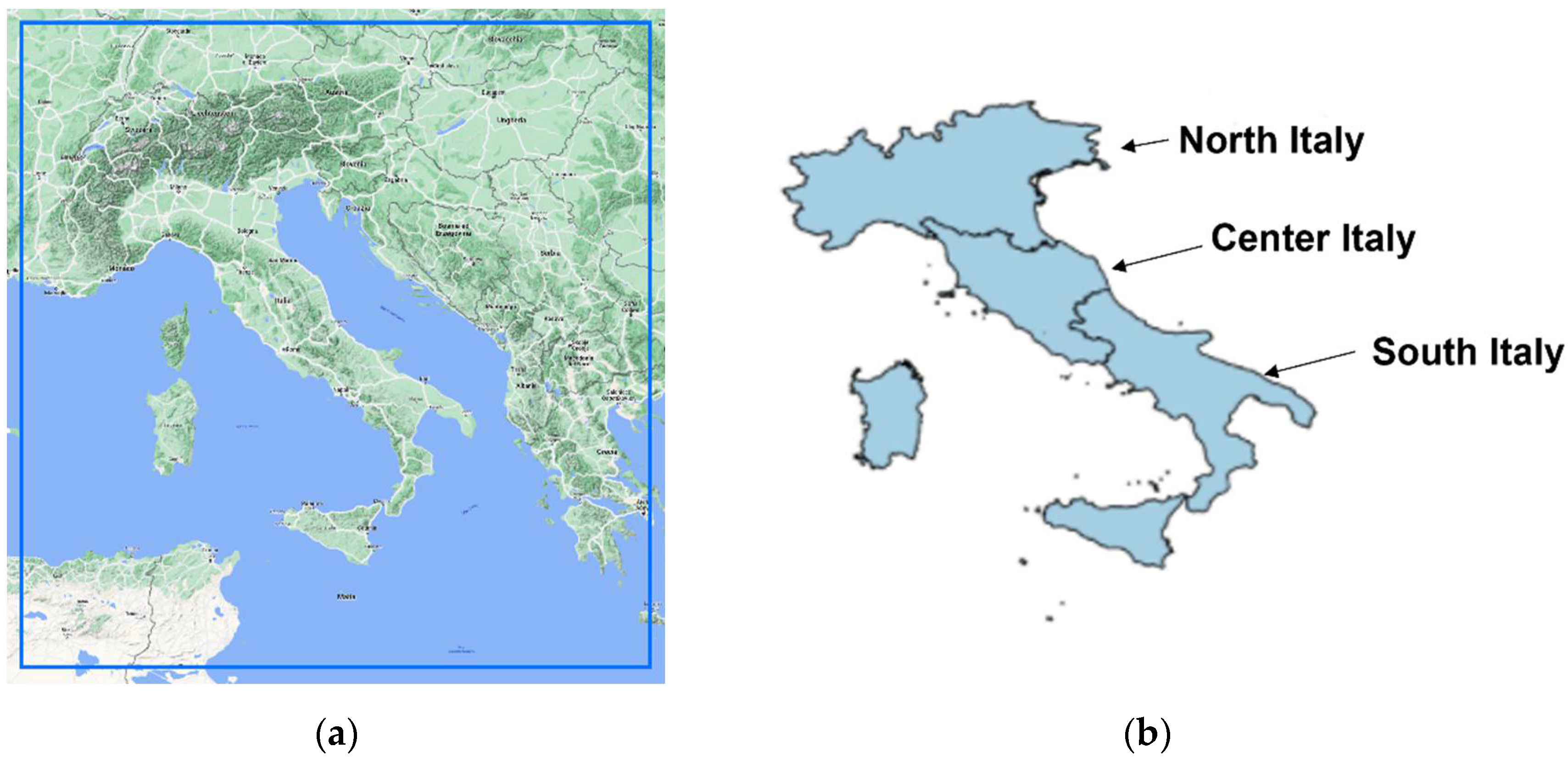
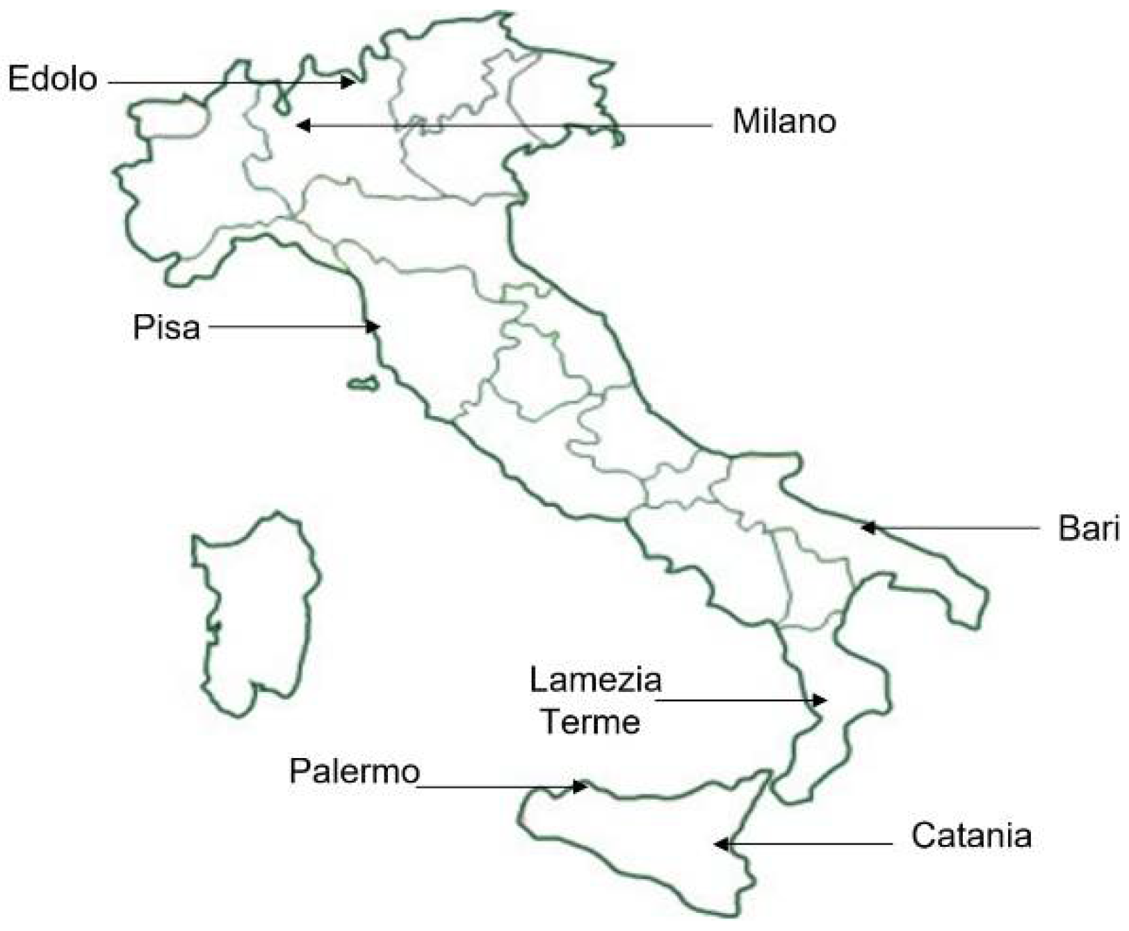
The domain considered in the present work is shown in Figure 1a and includes the whole Italian peninsula, extending from 34.199° N to 48.612° N and from 3.8056° E to 23.800° E. The positioning of boundaries was chosen in order to avoid crossing of mountain chains, improving the numerical stability. The computational grid is an R2B10 and is made up of 451,384 triangular cells, with a spatial resolution of about 2.5 km. The geometrical center of the grid is positioned in Gaeta (longitude 13.802° E, latitude 41.560° N).
Moreover, in order to perform a model sensitivity to the domain size, two additional domains were considered (D1 and D2, not shown), with the same geometrical center and the same resolution R2B10; however, with extensions larger, respectively, of 100 and 200 km with respect to the original one. D1 is made up of 498,712 cells, D2 of 562,240 cells.
Analysis was conducted over the Italian area, considering the second level of NUTS2 (Nomenclature des Unités Territoriales Statistiques) repartition but, for simplicity, in this work the sensitivity results are presented in the three macro-areas shown in Figure 1b.
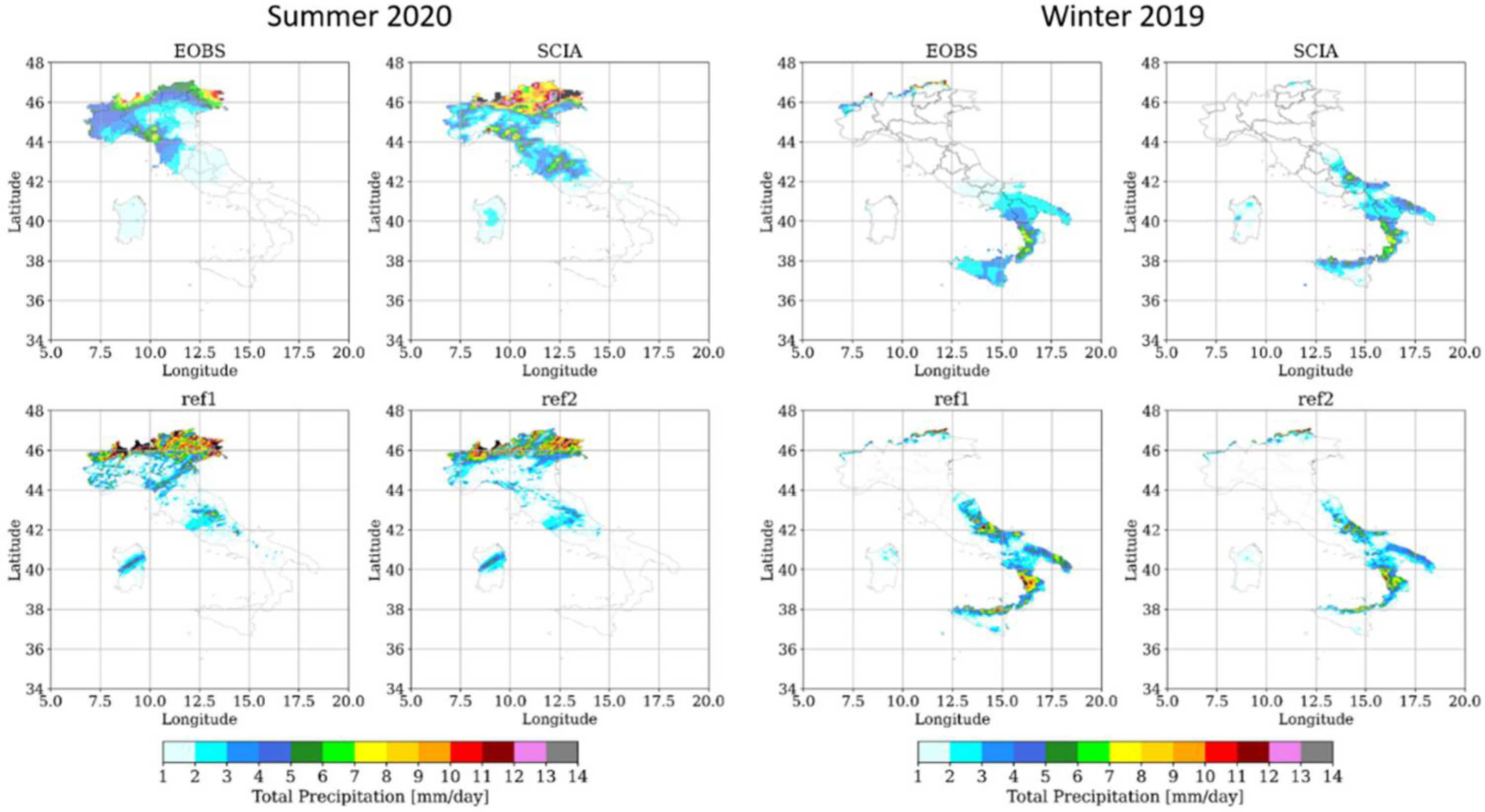
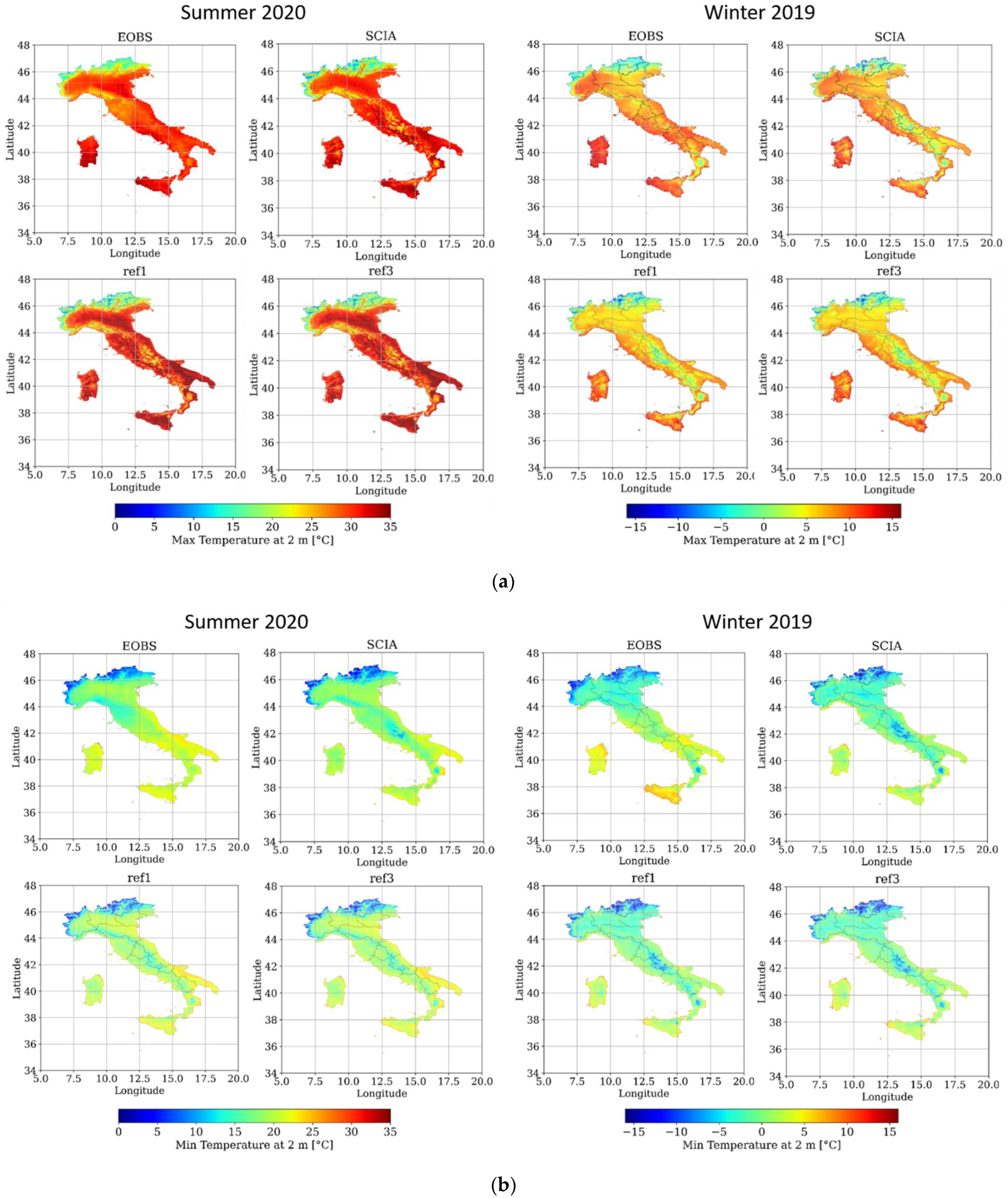
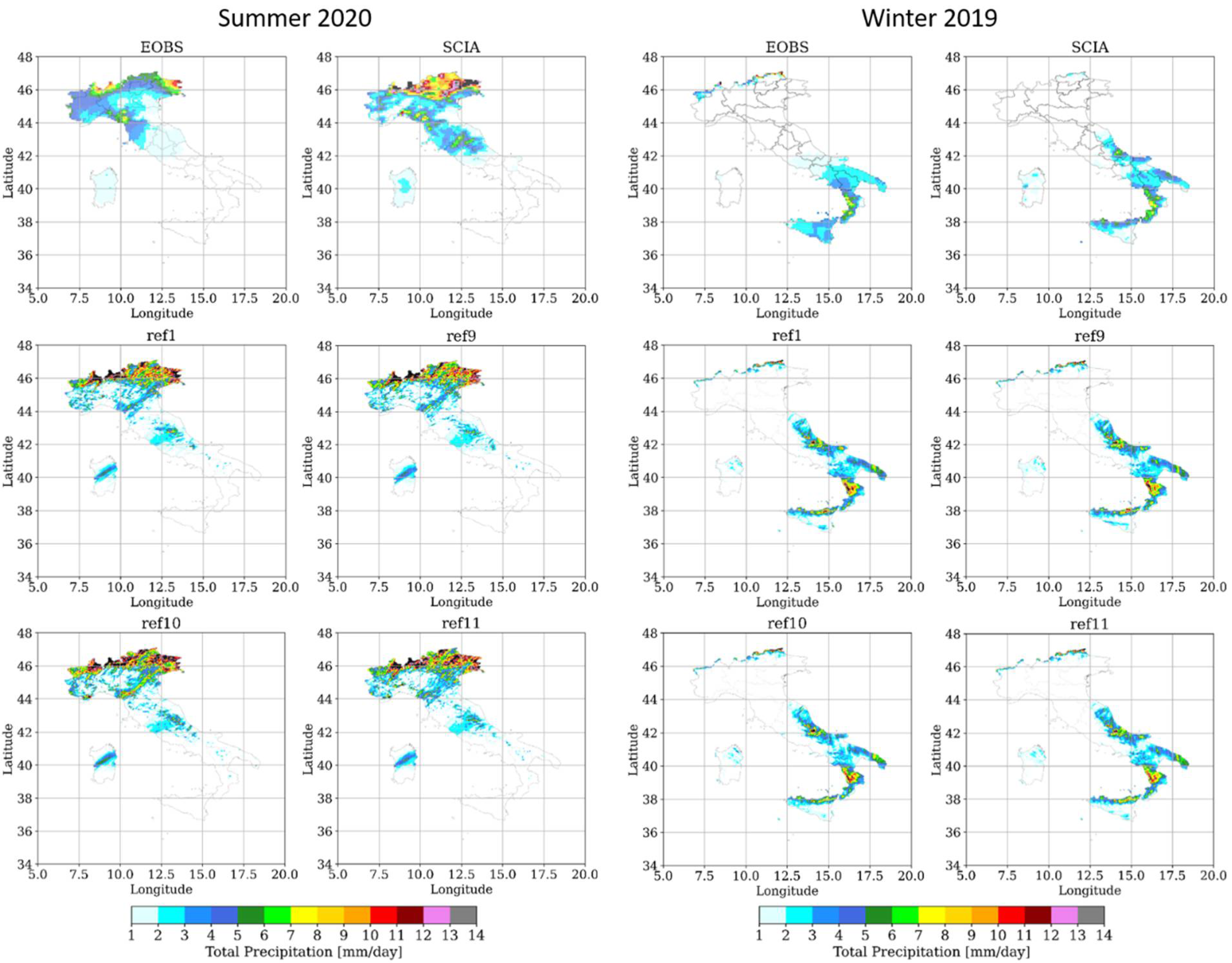
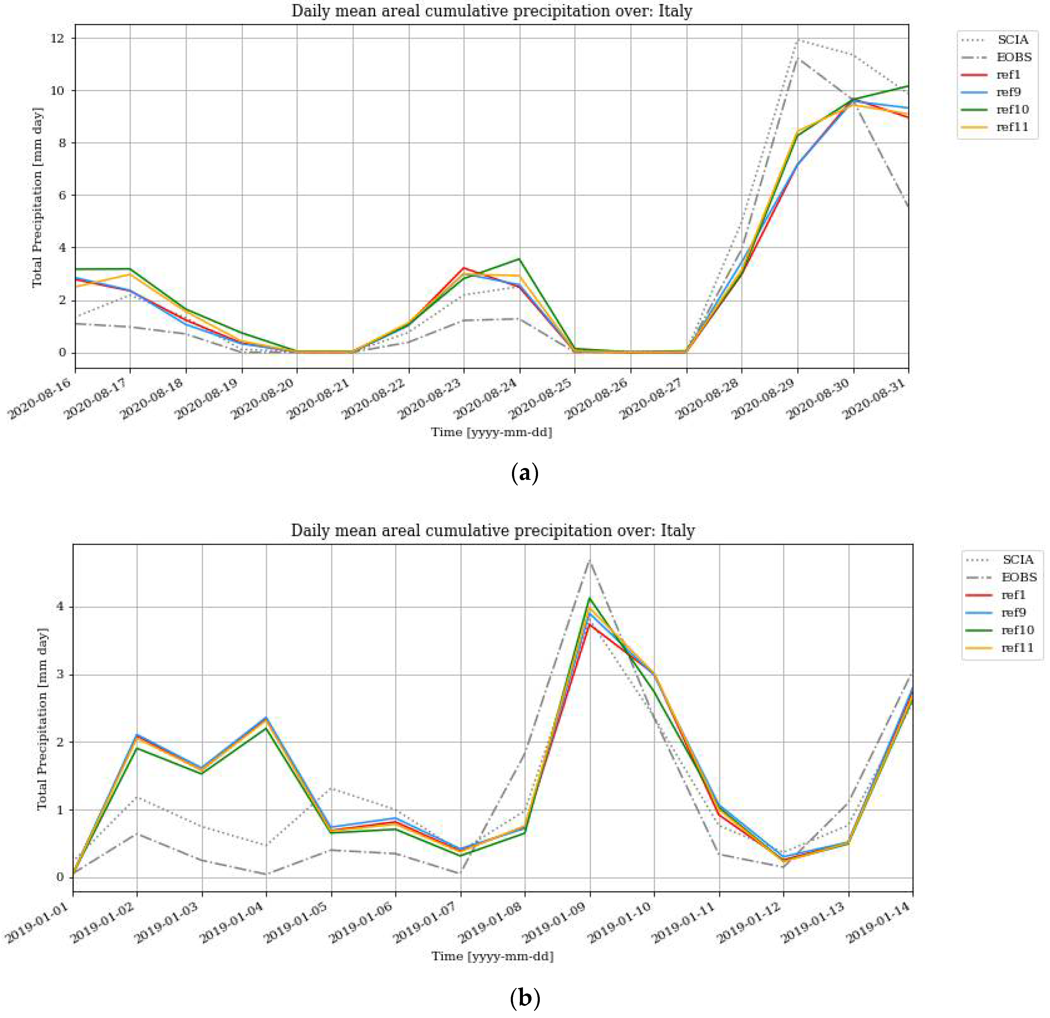
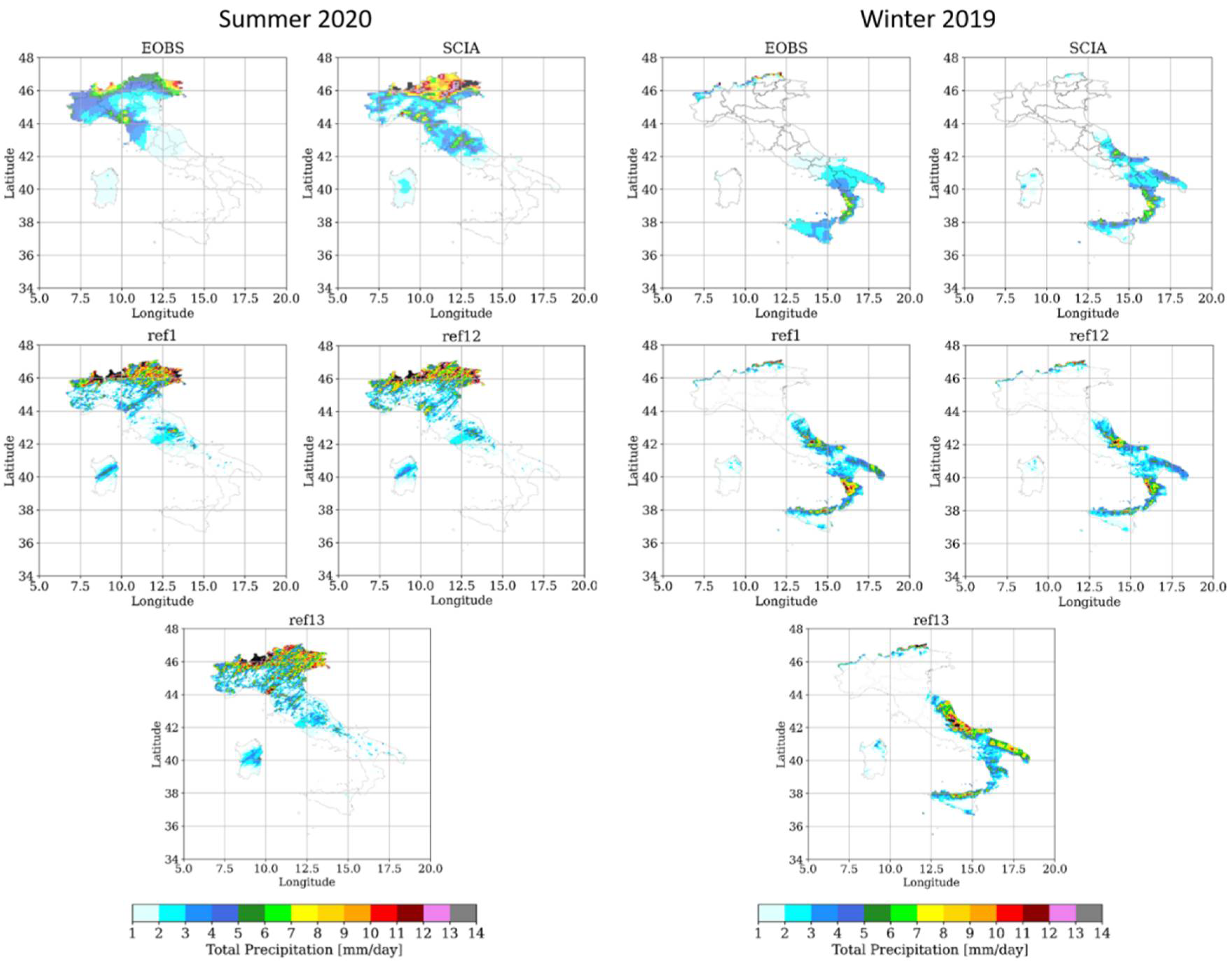
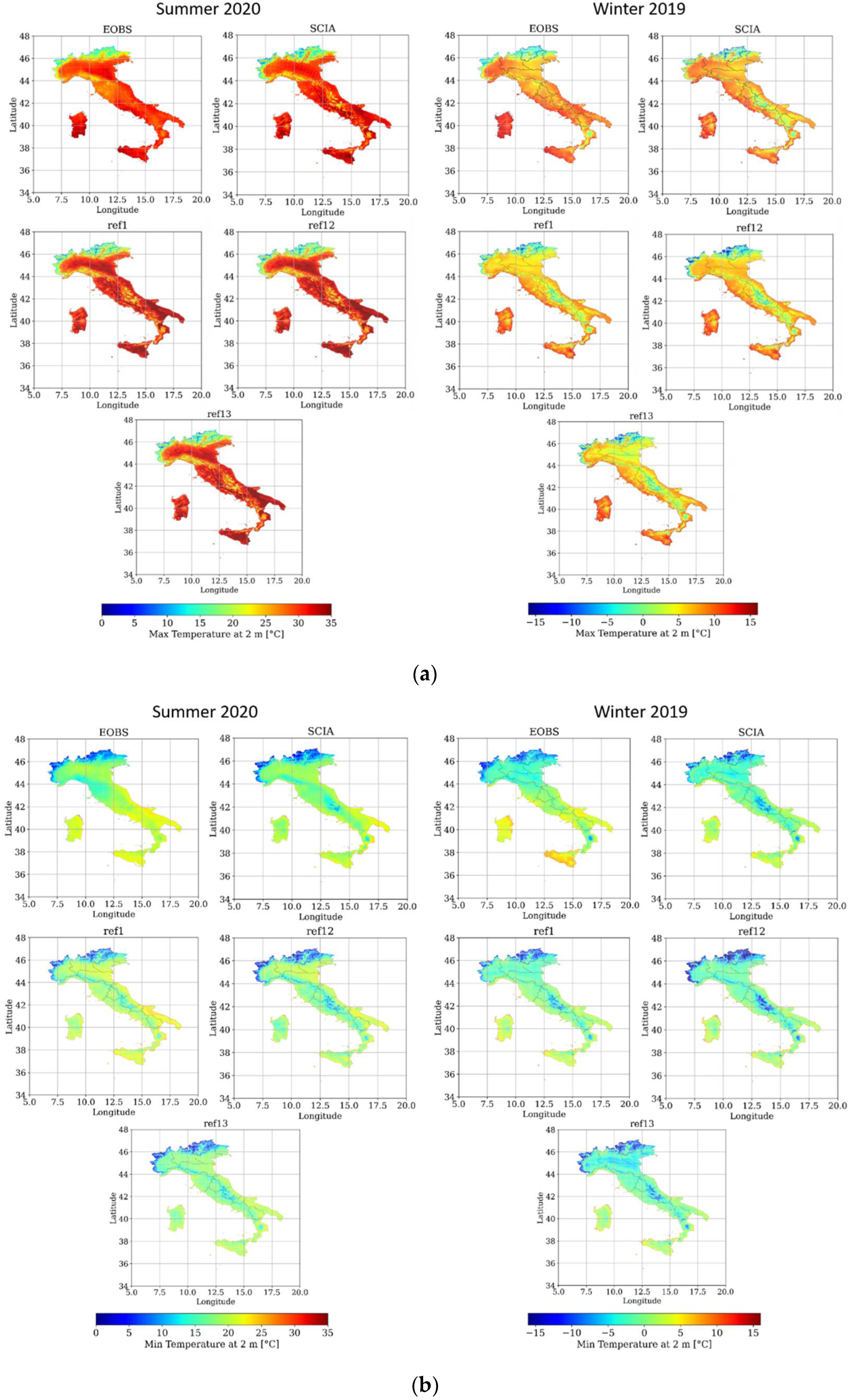
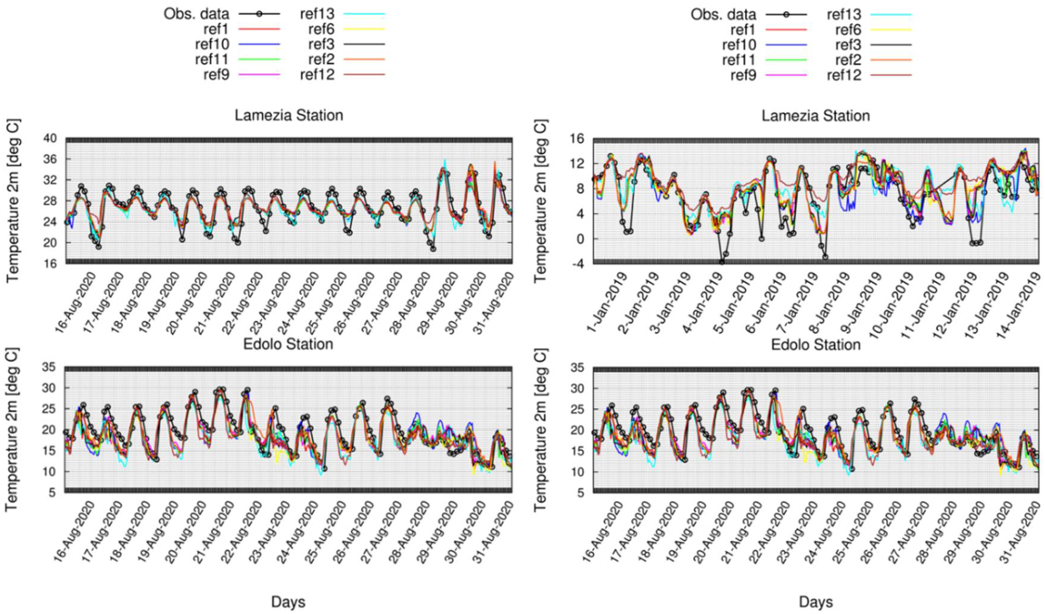
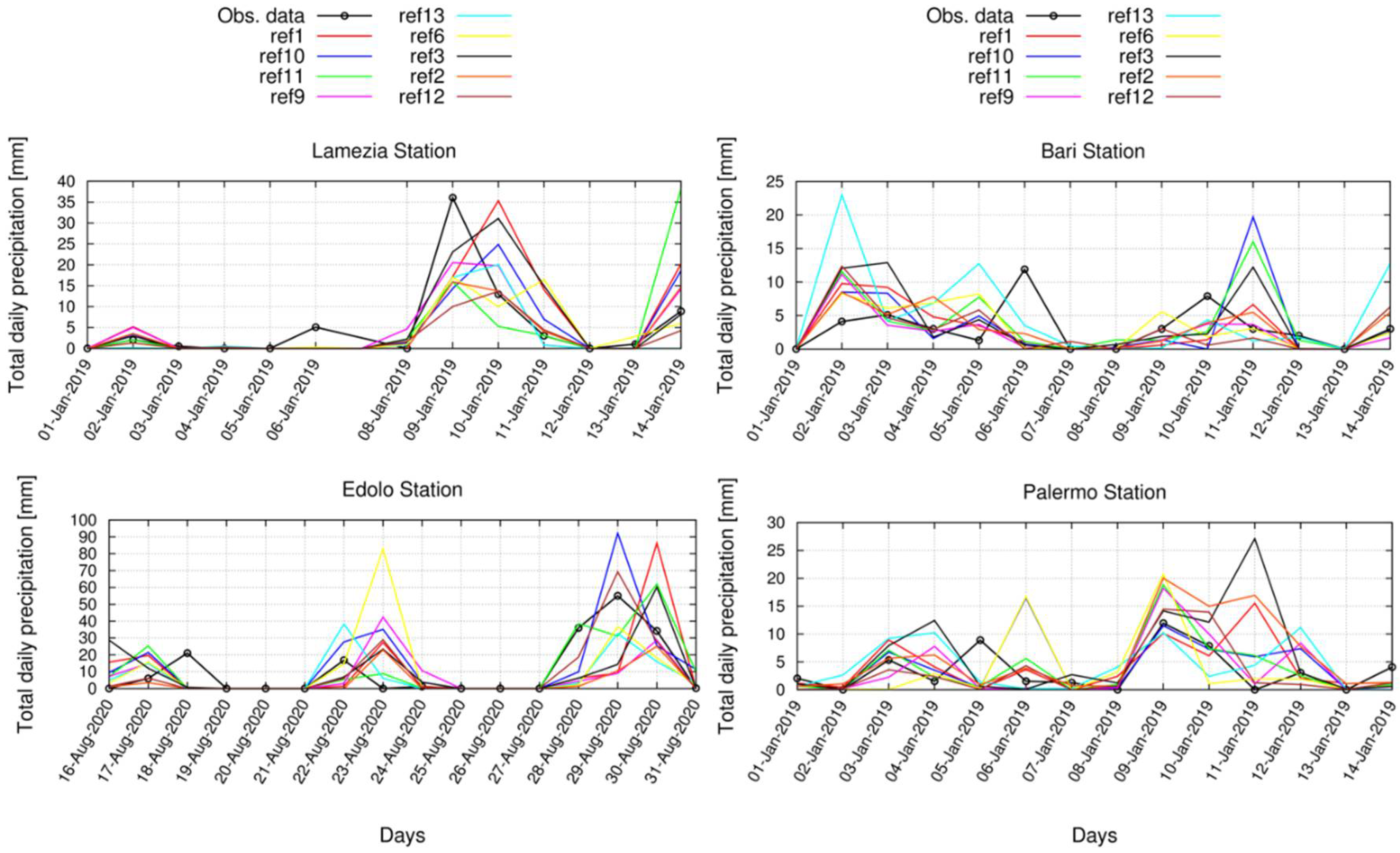
Two test cases were considered, namely 1–14 January 2019 and 16–31 August 2020. The selected periods were chosen in order to investigate the capabilities of ICON-LAM under different weather conditions and will be identified in the following as winter 2019 and summer 2020. The first period was characterized by several rainy events and strong winds, whereas the second one was characterized by an extreme precipitation event that occurred during 29 and 30 August 2020.
Specifically, hindcasts were initialized once and ran continuously throughout each of the 2-week periods. The initial and boundary conditions are the “analysis” provided by the ECMWF IFS model [9], characterized by a spatial resolution of 0.075° (about 8.5 km), with the boundary conditions updated every 6 h. This approach was chosen in order to have accurate boundary conditions and minimize the errors introduced by the forcing data, thus, avoiding a long-range error growth.
In any case, it is worth noting that initializing ICON with IFS data could be problematic for soil moisture, as the Land Surface Models used in both models have substantially different soil water climatologies. Model evaluation was executed considering the 2-m temperature (T2m) as the most basic weather variable and precipitation that, at convection permitting scales, is a fundamental parameter.
The simulations were performed on the Supercomputer ZEUS of the Fondazione Centro Euro-Mediterraneo sui Cambiamenti Climatici (CMCC). This is a Lenovo HPC cluster based on 348 Intel Xeon dual processor nodes (for a total of 12,528 cores) interconnected by means of an Infiniband EDR network. Due to the high performance of the supercomputer, each simulation over the domain considered employs less than 20 min for each day, using 576 cores distributed on 16 nodes.

2.2. Observational Datasets

Model evaluation was conducted against SCIA, a gridded observational dataset provided by the Italian Environmental Protection Agency (ISPRA) (http://www.scia.isprambiente.it/, accessed on 10 March 2022), available at a horizontal resolution of about 5 km for T2m and 10 km for precipitation over the whole Italian area. This dataset comes from the interpolation of data stations at daily resolution, covering the 20th century up to the present date (with different reliability due to the different number of interpolated values available each year) [10]. SCIA provides daily maximum and minimum values of T2m and daily precipitation values.
Additionally, the E-OBS [11] (version 23.1) was considered, a widely used gridded daily dataset of precipitation and temperature at 0.11° spatial resolution (about 11 km), available for the period 1950–2020, covering the European area (mean daily values). It is generally used for monitoring the climate in Europe (especially with regard to the assessment of daily extremes) and is an important dataset for model validations, even if, for the present work, some shortcomings are expected, related to the large difference of resolution between the model and the dataset.
Moreover, in order to strengthen the analysis, evaluation was conducted also against selected data stations provided by regional environmental protection agencies (ARPA) scattered over the Italian area, since non-negligible errors could affect gridded data, especially in mountainous regions, since the majority of stations are located in valleys, and the assumptions made for the height regression may not be appropriate on individual days.

2.3. Methodology

The sensitivity analysis was conducted starting from a reference configuration developed at DWD and modified according with the finding of Khain P. (2021, personal communication) obtained over Israel. The external datasets used are GLC2000 for land use, GLOBE for surface altitude and FAO Digital Soil Map of the World for soil types. The convection scheme is the classical Tiedtke/Bechtold, whereas the land surface scheme is the multi-layer model TERRA [12], which simulates the energy and water balance at the land surface and in the ground, providing the lower boundary-condition for the atmospheric model and is responsible for the exchange of fluxes of heat, moisture and momentum between land surface and atmosphere.
Other main features are:
-
The time step dt was set equal to 24 s. This value was chosen after a series of preliminary tests. In particular, it was shown that the value 36 s does not guarantee stability, whereas the value 12 s provides almost the same solution as with 24 s.
-
The number of vertical levels was set equal to 65 as a tradeoff between accuracy and computational costs after preliminary tests were performed also with 50 and 90 vertical levels. The highest level was at 22 km.
ICON allows choices to be made among different parameterizations of physical phenomena and numerical schemes as well as the selection of suitable values for parameters related to them. It is therefore possible to optimize the configuration of the model according to the climatology of the area and the spatial resolution employed.
In the present work, starting from the reference configuration described above, different configurations were defined by varying one scheme (parameter) at a time. A list of the sensitivity runs with changes in the parameters with respect to the control run (ref1) is reported in Table 1. According with previous experiences on sensitivity analysis [13], sensitivity tests mainly regard the physics schemes and are combined into five groups.
Sensitivity to convection: Convection is a fundamental process in the atmosphere, since it contributes to the formation of large-scale circulation and local heavy precipitation. In ICON, it is parameterized through a bulk mass flux scheme based on Tiedtke/Bechtold [14] (the parameter inwp_convection is set to the value 1). In the reference configuration (named ref1 in Table 1), the shallow convection parameterization is active whereas the parts treating deep and mid-level convection are switched off (the parameter lshallowconv_only is set to TRUE). This option is recommended for convection permitting grids (resolution between 1 and 3 km). The second option (adopted in ref2 of Table 1) adopts a full convection scheme (both kinds of convection are parameterized). In such a case, the parameter lshallowconv_only is set to FALSE.
Sensitivity to the radiation scheme: Radiation is an important component of a weather model, since local and global temperatures are determined by heating (absorption) and cooling (emission). The shortwave radiation from the sun and the longwave radiation from the earth interact with clouds. The reference configuration (ref1 in Table 1) uses the radiation scheme ecRad [15,16] and the parameter inwp_radiation is set to the value 4.
This allows choices for each component, namely the optical property parameterizations for the atmospheric components and the radiation solver calculating how radiation travels through the optical medium. A second option (adopted in the case ref3 of Table 1) uses a rapid and accurate radiative transfer model RRTM [17] and the parameter inwp_radiation is set to the value 1. Moreover, the options with Ritter-Geleyn radiation [18] and PSRAD [19] are also tested in cases ref4 and ref5 of Table 1, respectively, and the parameter inwp_radiation is set to the values 2 and 3, respectively.
Sensitivity to the cloud microphysics schemes: they are made up of a closed set of equations able to calculate the formation and evolution of condensed water in the atmosphere. These provide the latent heating rates for the dynamics. The reference configuration (ref1 in Table 1) uses a single moment scheme, which predicts the cloud water, rain water, cloud ice, snow and graupel [12], and the parameter inwp_gscp is set to the value 2.
A second option (adopted in the case ref6 of Table 1) is based on a double moment scheme, which predicts the mass and number of cloud water, rain water, cloud ice, snow, graupel and hail [20] and the parameter inwp_gscp is set to the value 4. This scheme is mainly recommended at convection permitting scales, i.e., mesh size smaller than 3 km. Further options (adopted in the cases ref7 and ref8 of Table 1) are based on the Koehler scheme (improved ice nucleation) and on the Kessler scheme [21] and the parameter inwp_gscp is set to the value 3 and 9, respectively.
Sensitivity to cloud cover: an estimate of cloud cover is required to prepare optical properties of clouds for the radiative transfer. The reference configuration (ref1 in Table 1) uses a diagnostic cloud cover scheme (Kohler), which combines information from turbulence, convection and microphysics schemes, and the parameter inwp_cldcover is set to the value 1. A second option (adopted in the case ref9 of Table 1) is based on the COSMO SGS cloud scheme (cloud cover and cloud water/ice calculation are performed as in the COSMO model), and the parameter inwp_cldcover is set to the value 3.
A third option (adopted in the case ref10 of Table 1) is clouds as in turbulence approach, in which the area fraction of a grid box covered by stratiform (non-convective) clouds is calculated; an additional saturation adjustment is done assuming a Gaussian distribution for the saturation deficit. In such a case, the parameter inwp_cldcover is set to the value 4. The last option (adopted in the case ref11 of Table 1) is a simple grid scale cloud cover, in which each computational cell is marked with 1 or 0, according to the presence (or not) of clouds; this is determined by comparing the specific cloud water/ice content of each cell with an assigned threshold value (the parameter inwp_cldcover is set to the value 5).
Sensitivity to the turbulence transfer: this parameterization links the resolvable scales and the non-resolvable fluctuating scales of motion. Turbulent fluxes run an exchange of momentum, heat and humidity between the free atmosphere and the earth’s surface, representing a crucial issue for a proper simulation of atmospheric flows. The reference configuration (ref1 in Table 1) uses a turbulence scheme [22] taken from COSMO, based on a prognostic equation for Turbulent Kinetic Energy also considering that some modifications for ICON are still ongoing in order to improve the numerical stability under extreme conditions. In this case, the parameter inwp_turb is set to the value 1.
Another option (adopted in the case ref12 of Table 1) is based on the Globales Modell (GME) turbulence scheme [23], and the parameter inwp_turb is set to the value 2. The last option (adopted in the case ref13 of Table 1) is based on the 3D sub-grid model of Smagorinsky [24] implemented for Large Eddy Simulations applications, and the parameter inwp_turb is set to the value 5.
Statistical measures for model’s performance were calculated as the Root Mean Square Error (RMSE) and Mean Absolute Error (MAE), defined in the following, where S and O refer to daily values of model and reference product, respectively:
R M S E = 1 N i = 1 N ( S i O i ) 2
M A E = 1 N i = 1 N | S i O i |
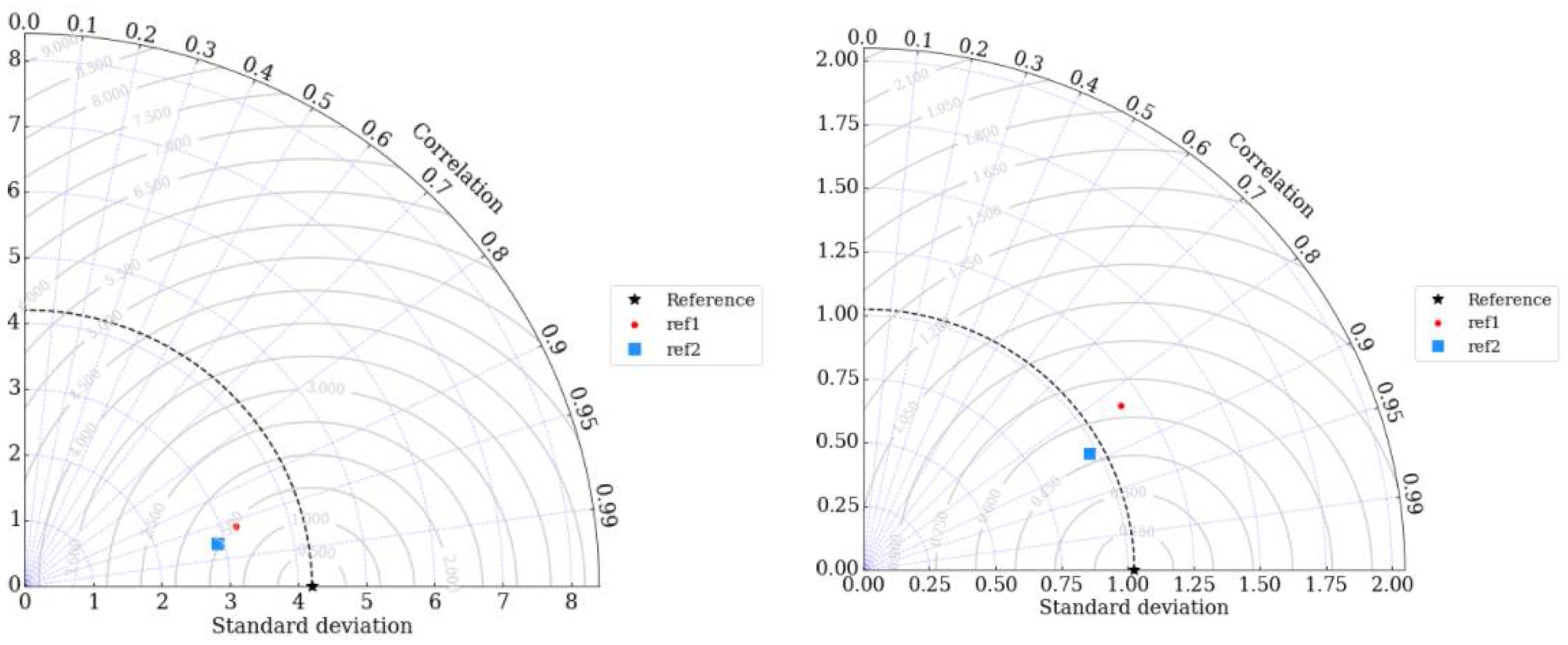
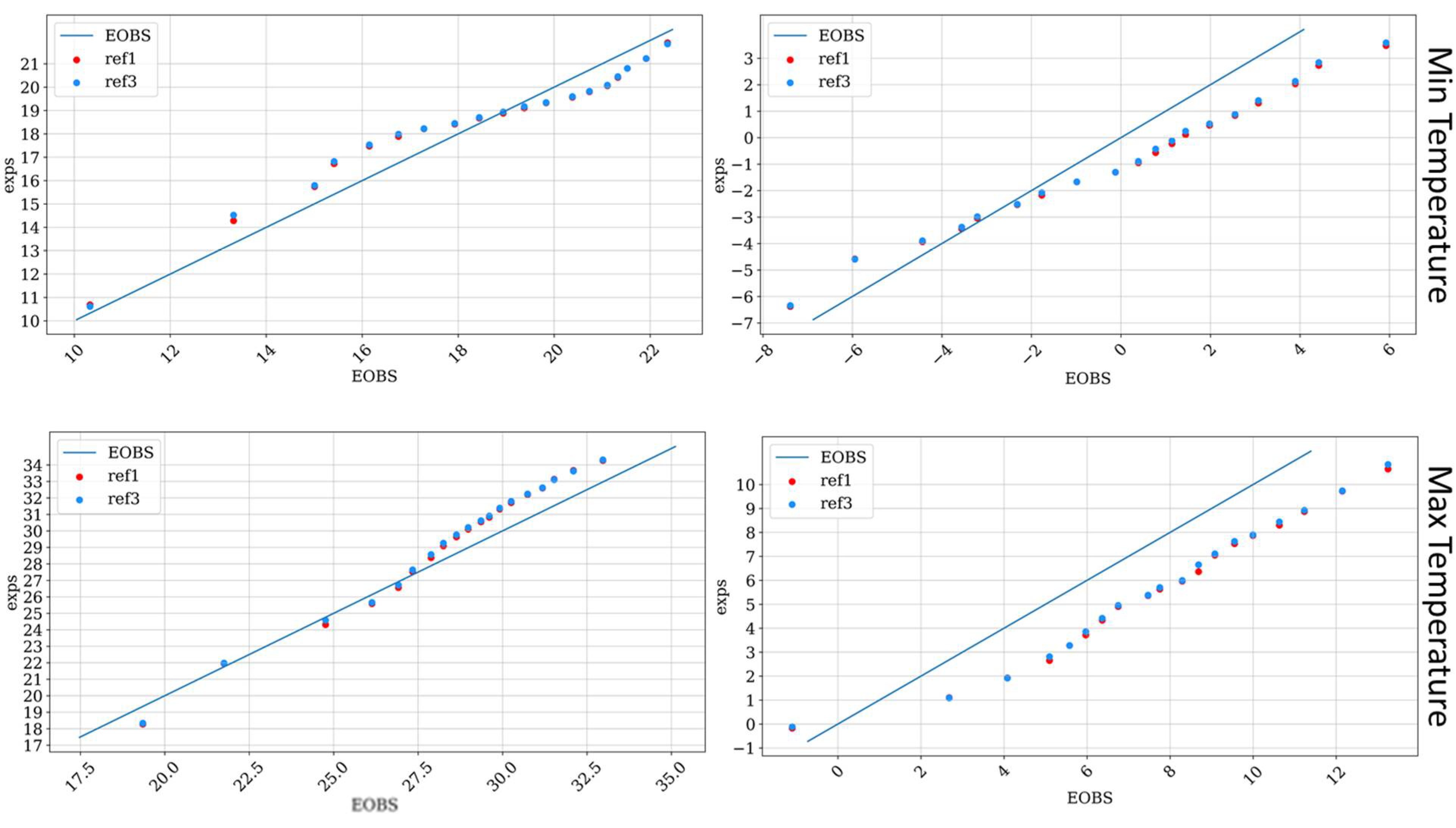
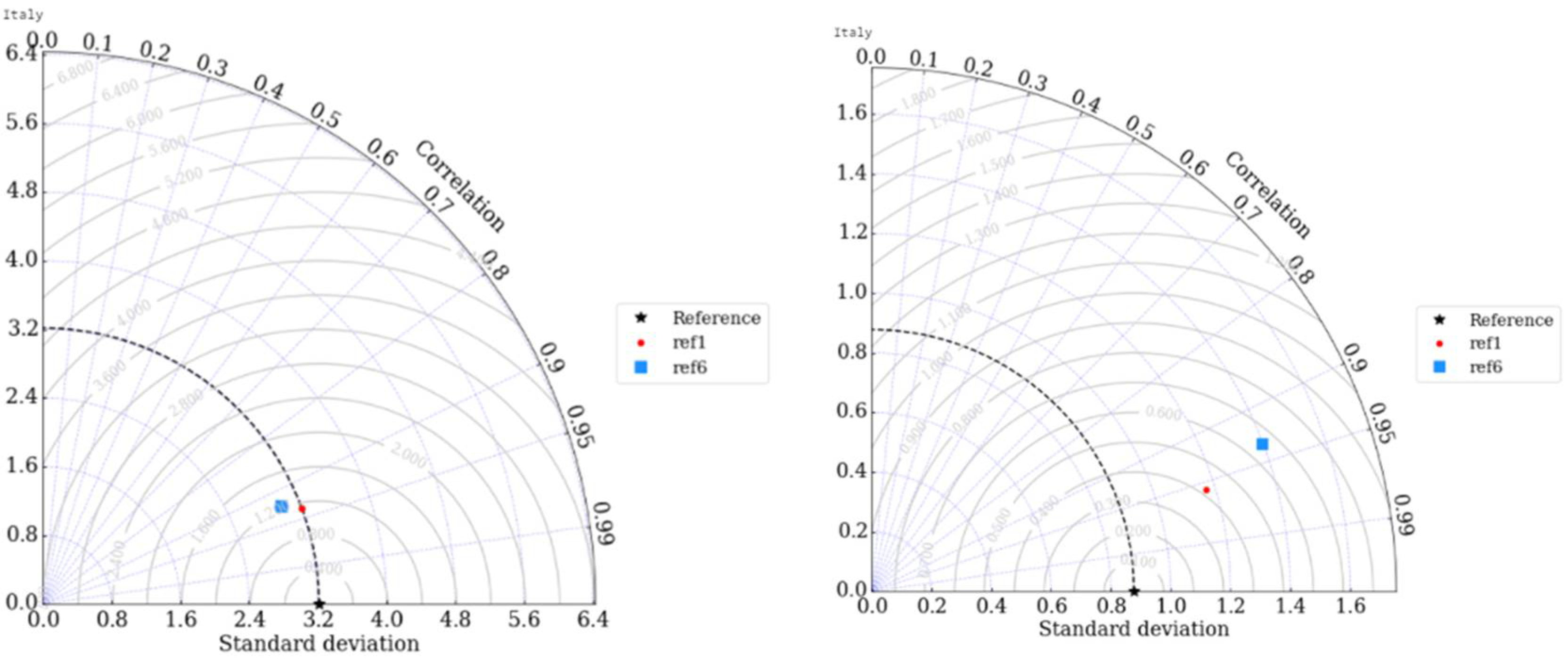
Here, N represents the number of grid points included in the macro area considered. Moreover, Taylor diagrams and Quantile-quantile plots (QQplot) are proposed. Taylor diagrams provide a graphical framework that allows a comparison among models and reference data in terms of their correlation, their root-mean-square difference and the ratio of their variances. QQ-plots use a graphical method and allow comparison of the probability distributions by plotting their quantiles against each other. If the compared distributions are close to the observations, the points in the QQplot approximately lie close to the 45° inclined line.

3. Results

The results are presented for each parameterization group in terms of T2m and/or precipitation depending on which variable is mainly affected by the schemes considered.

3.1. Sensitivity to Convection

A first analysis was performed comparing the results of the simulations ref1 and ref2, characterized by the usage of shallow convection only and full convection, respectively. Figure 2 shows the distribution of daily precipitation averaged over the two periods considered (summer 2020 on the left and winter 2019 on the right), respectively, provided by E-OBS, SCIA, ref1 and ref2.
The maps show that, in summer 2020, the two datasets are characterized by discrepancies over the Alpine area. The E-OBS precipitation data were assessed over the Greater Alpine Region by Turco et al. [25], and they showed that E-OBS does not provide reliable climatology over this area, and thus it must be treated with caution. Assuming SCIA as the main reference, both ref1 and ref2 underestimate precipitation over the Alpine area; however, simulation ref1 provides better performances, as confirmed by the indicators RMSE and MAE evaluated against SCIA (Table 2). This is due to the explicit treatment of deep convection and the more realistic model dynamics, confirming that (as shown also in [3]) the representation of summer precipitation benefits from the usage of convection-permitting simulations.
In winter 2019, ref1 overestimates the precipitation over southern-central Italy, while ref2 is able to reduce this bias, even if the differences between the two simulations are generally limited to 1 mm/day. Figure 3 shows the Taylor diagrams related to the whole domain over the two periods considered for ref1 and ref2, assuming SCIA as a reference, revealing that ref1 performs better in summer 2020 also in terms of the correlation and standard deviation, thus, confirming the importance of switching off the deep convection in summer season, whereas in winter the full parameterization clearly appears as the best choice.

3.2. Sensitivity to Radiation Scheme

A second analysis was conducted considering different radiation schemes, comparing the results of the simulations employing, respectively, ecRad (ref1) and RRTM (ref3). Other options (Ritter-Geleyn radiation-ref4 and PSRAD-ref5) did not provide reliable results and are not presented. Figure 4 shows the distribution of daily maximum (a) and minimum (b) T2m values averaged over summer 2020 on the left and winter 2019 on the right, respectively, provided by E-OBS, SCIA, ref1 and ref3. A discrepancy between the two observational datasets is recorded, especially over Tuscany in summer and over Apennine chain in winter. A deeper investigation performed considering station data used in the present work has revealed that E-OBS is affected by larger errors in some areas and that SCIA is generally more reliable.
In summer 2020, both the simulations are in good agreement with SCIA; however, an overestimation over Tuscany and some regions in the south (in particular Puglia and Campania) is recorded. This warm bias is due to the difficulties of the model in reproducing atmospheric dynamics typical of central Italy (e.g., surface-based temperature inversions) [26] and was also observed for COSMO-CLM [27]. In winter, an underestimation of temperature is registered, especially at high altitudes and could be related to inadequate representation of complex orographic areas [28]. The analysis of indicators (Table 3) reveals that the differences of performances between the two schemes are minimal, with a slightly better behavior of ref1 in summer 2020.
Figure 5 shows the QQplot of daily maximum and minimum T2m (summer 2020 on the left and winter 2019 on the right) of both configurations against E-OBS data. This plot reveals that in summer both configurations tend to overestimate the maximum T2m, while in winter both maximum and minimum temperatures are underestimated (with the exception of very cold values).

3.3. Sensitivity to Cloud Microphysics

The next analysis was performed comparing different microphysics schemes, specifically the single moment (ref1) and the double moment one (ref6), since other options (the Koehler scheme-ref7 and the Kessler scheme-ref8) were affected by instability problems and did not provide reliable results. Figure 6 shows the distribution of daily precipitation averaged over the two periods considered (summer 2020 on the left and winter 2019 on the right), respectively, provided by E-OBS, SCIA, ref1 and ref6.
As already discussed, in summer 2020 ref1 underestimates the precipitation over the Alpine area whereas the almost null precipitation over southern Italy is well reproduced. As confirmed also by the numerical values of RMSE and MAE (Table 4), ref6 is not able to improve the model performances. In winter 2019, ref1 overestimates precipitation over southern-central Italy and also in this season ref6 is characterized by worse performances over the three areas. These findings are also confirmed by the Taylor diagrams (Figure 7), showing that ref1 performs better in both seasons also in terms of correlation and standard deviation.

3.4. Sensitivity to Cloud Cover

In this subsection, a comparison among different cloud cover schemes is analyzed, specifically diagnostic cloud cover (ref1), COSMO SGS scheme (ref9), clouds as in turbulence (ref10) and grid scale cloud cover (ref11). Figure 8 shows the distribution of daily precipitation averaged over the two periods considered (summer 2020 on the left and winter 2019 on the right), respectively, provided by E-OBS, SCIA, ref1, ref9, ref10 and ref11. In summer 2020, the problem of underestimation over the Alpine region with ref1 is slightly mitigated by the other schemes and in particular by ref11, as the RMSE over North Italy is reduced from 3.3 to 2.6 mm/day (Table 5).
Over the other areas, no relevant differences among the configurations are recorded. In winter 2019, better performances are achieved with ref10, which allows a RMSE reduction in Central Italy from 0.5 to 0.4 and South Italy from 1.9 to 1.7. Figure 9 shows the time series of daily precipitation values (averaged over the whole domain) obtained with the different configurations and observational data, for summer 2020 (a) and winter 2019 (b).
These figures reveal the good capabilities of the model in reproducing the daily variability of precipitation, especially the peaks recorded in winter period, whereas the intense precipitation event of 29–30 August 2020 is partially underestimated by all the configurations tested. Table 5 provides also the numerical values of indicators for daily maximum and minimum temperature (°C) against SCIA, showing that ref11 is able to reduce the strong winter bias affecting Tmax, over Central and South Italy; for the minimum temperature, the different schemes generally perform in a similar manner.

3.5. Sensitivity to the Turbulent Transfer

The last sensitivity analysis was performed comparing the different turbulence schemes implemented, namely the COSMO diffusion and transfer (ref1), the GME turbulence scheme (ref12) and the classical Smagorinsky diffusion (ref13). This kind of parameterization has relevant effects on both the T2m and precipitation. Figure 10 shows the distribution of daily precipitation, averaged over the two periods considered (summer 2020 on the left and winter 2019 on the right) provided by E-OBS, SCIA, ref1, ref12 and ref13. In summer 2020, precipitation is underestimated over North Italy by all the three configurations, whereas, over the other areas, good performances are generally achieved, especially with ref13 over Central Italy (see also numerical values in Table 6). In winter 2019, the overestimation over South Italy is partially mitigated by ref12, while ref13 introduces an additional overestimation.
Figure 11 shows the distribution of the daily maximum and minimum T2m values averaged over summer 2020 (on the left) and winter 2019 (on the right). In summer 2020, ref13 is characterized by smaller RMSE and MAE values (Table 6), and thus the usage of the classical Smagorinsky diffusion is recommended. In contrast, in winter 2019, ref12 and ref13 are not able to improve the performances over the three areas, and thus the “COSMO diffusion and transfer” is recommended.

3.6. Evaluation against Station Data

In order to endorse the results achieved, model evaluation was conducted also against data provided by stations scattered over the Italian area (Figure 12). These were chosen in order to test the model performances under different climate and orographic conditions. Figure 13 shows the time series of T2m for selected stations and periods obtained with the different configurations and observational data.
In Lamezia Terme (summer 2020), the amplitude of diurnal cycle is generally underestimated, with slight improvements provided by the Smagorinsky diffusion for turbulent transfer (ref13), while, in winter 2019, the daily maximum values are well captured; however, minimum ones are overestimated; the clouds as in turbulence (ref10) scheme seems to improve the performances in this sense, as confirmed also by the low RMSE value (see Table 7). In Edolo (located at altitude 700 m), the daily maximum and minimum values are underestimated by all the configurations in both the periods, confirming the temperature cold bias observed in mountainous areas against SCIA dataset, partially reduced only by ref2.
Figure 14 shows the time series of precipitation for selected stations and periods obtained with the different configurations and observational data. In Lamezia Terme (winter 2019), the model has difficulties in capturing the intense precipitation of 9 January, the related peak is delayed by all the configurations. In Bari (winter 2019), the daily variability is quite well captured by most of the configurations but with a marked overestimation in some days. A similar trend is recorded in Edolo (summer 2020) and Palermo (winter 2019); however, in these two cases, the GME turbulence scheme provides relevant improvements.
Table 7 shows the values of the RMSE of daily T2m (°C) and precipitation (mm/day) for the selected stations and for the different model configurations, averaged over the two periods. These values confirm that, for precipitation, the explicit treatment of deep convection allows better performances in summer, with the exception of Edolo, where a strong error is recorded for all the configurations. The results confirm that the ecRad scheme provides better performances in summer for both variables (with the exception of Edolo).
Regarding cloud microphysics, the results confirm the better behaviour of the single moment scheme. An interesting result is observed for the grid scale cloud cover scheme, which is able to reduce the strong precipitation bias over mountain areas in summer, also providing better performances for T2m in both seasons. Finally, both the GME turbulence scheme and the classical Smagorinsky diffusion are able to reduce the precipitation bias over mountain areas in summer, also providing good improvement in winter.

4. Discussion and Conclusions

The main aim of this study was to provide a preliminary analysis to assess the sensitivity of ICON-LAM parameterizations over the Italian area at about 2.5 km of spatial resolution and produce an optimal parameterization combination for the investigated area. Simulations were performed in a computational environment that is quite different from the facilities where ICON was developed, and thus a large IT effort was required. The long term purpose of this activity is to calibrate ICON-LAM in the best way, defining a set-up to be used as a numerical weather prediction system for Italy.
Since ICON-LAM is a “new-born” model, only a few preliminary studies have been conducted to investigate the performance of the various available physical parameterizations over a complex geographic region, such as the Italian area; therefore, this work was aimed to provide a contribution to the selection of model parameters (and their values) that result to be more effective for a proper representation of the Italian climate features. This first assessment requires further deeper analyses that will be performed in the future, by using an objective calibration approach, such as the one developed in the frame of the COSMO CALMO project.
The present analyses revealed that the reference ICON configuration provided by DWD has good capabilities in reproducing the most basic meteorological variables over Italy, considering the different datasets adopted. Values of T2m show a general good agreement with observations, being an average bias generally lower than 1 °C, with the exception of the strong warm bias over Tuscany, which is partially reduced by the alternative parameterization schemes tested but needs further investigations. Small improvements can be achieved in winter over central-south Italy using the classical Smagorinsky diffusion for turbulent transfer and the grid scale cloud cover.
Regarding precipitation, the analysis performed confirms that a reduction of the underestimation over the Alpine region can be achieved with the explicit treatment of deep convection. The single moment scheme is currently the best option for cloud microphysics, even if alternative options (the Koehler and the Kessler schemes) need further attention in the near future in order to highlight their potential capabilities.
Regarding cloud cover, the “clouds as in turbulence” scheme allows a bias reduction in summer over the Alpine region and is the best choice for this kind of parameterization. Finally, a proper choice of the turbulence is crucial for a good representation of both T2m and precipitation fields. The analysis performed suggests that the usage of the classical COSMO diffusion and transfer scheme is currently recommended; however, further tests are needed, since turbulence is a standalone source of investigation.
The observed biases are certainly due to shortcomings of the model in simulating meteorological features of the Italian area; however, deficiencies in the lateral boundary conditions and internal variability play also a relevant role, as well as inaccuracies of the gridded observational datasets affected by errors introduced with numerical interpolations. For this reason, in this work, an evaluation of ICON-LAM was also performed against observational data from selected stations scattered over Italy in order to strengthen the analysis, and the results generally confirm the findings of the sensitivity performed considering gridded data. However, in a future work, specific analyses will be performed over a larger number of selected locations, even considering different resolutions, in order to highlight also the benefits of higher grid resolutions.

Author Contributions

Conceptualization, E.B., P.M. and C.D.L.; methodology, C.D.L.; software, A.M. and D.C.; validation, C.D.L., M.A., D.C. and M.M.; formal analysis, P.M.; investigation, C.D.L.; resources, A.M. and P.S.; data curation, M.A., C.D.L., P.S. and A.M.; writing—original draft preparation, E.B.; writing—review and editing, all; visualization, C.D.L., M.M. and D.C.; All authors have read and agreed to the published version of the manuscript.

Funding

This research received no external funding.

Institutional Review Board Statement

Not applicable.

Informed Consent Statement

Not applicable.

Data Availability Statement

Data stored at CMCC supercomputing center and available on request.

Acknowledgments

The authors would like to thank Daniel Rieger (DWD) for the continuous support provided in the execution of numerical simulations and the “Servizio Idro-Nivo-Meteo e Clima di ARPA Lombardia” for providing observational data over Lombardia. The authors thank the national and regional Italian agencies that contribute to feed the SCIA system (www.scia.isprambiente.it, accessed on 10 March 2022) with the data used in the present work.

Conflicts of Interest

The authors declare no conflict of interest.

References

  1. Zängl, G.; Reinert, D.; Rípodas, P.; Baldauf, M. The ICON (icosahedral non-hydrostatic) modelling framework of DWD and MPI-M: Description of the non-hydrostatic dynamical core. Q. J. R. Meteorol. Soc. 2015, 141, 563–579. [Google Scholar] [CrossRef]
  2. Arakawa, A.; Lamb, V.R. Computational Design of the Basic Dynamical Process of the UCLA General Circulation Model. Methods Comput. Phys. 1977, 17, 173–265. [Google Scholar] [CrossRef]
  3. Steppeler, J.; Doms, G.; Bitzer, H.W.; Gassmann, A.; Damrath, U.; Gregoric, G. Meso-gamma scale forecasts using the nonhydrostatic model LM. Theor. Appl. Clim. 2003, 82, 75–96. [Google Scholar] [CrossRef]
  4. Pham, T.V.; Steger, C.; Rockel, B.; Keuler, K.; Kirchner, I.; Mertens, M.; Früh, B. ICON in Climate Limited-area Mode (ICON release version 2.6. 1): A new regional climate model. Geosci. Model Dev. 2021, 14, 985–1005. [Google Scholar] [CrossRef]
  5. Rieger, D.; Milelli, M.; Boucouvala, D.; Gofa, F.; Iriza-Burca, A.; Khain, P.; Kirsanov, A.; Linkowska, J.; Marcucci, F. Verification of ICON in Limited Area Mode at COSMO National Meteorological Services; Reports on ICON n.6; DWD Publication: Offenbach am Main, Germany, 2021. [Google Scholar] [CrossRef]
  6. Sakradzija, M.; Klocke, D. Physically constrained stochastic shallow convection in realistic kilometer-scale simulations. J. Adv. Model. Earth Syst. 2018, 10, 2755–2776. [Google Scholar] [CrossRef]
  7. Avgoustoglou, E.; Voudouri, A.; Khain, P.; Grazzini, F.; Bettems, J.M. Design and Evaluation of Sensitivity Tests of COSMO model over the Mediterranean area. Perspect. Atmos. Sci. 2017, 1, 49–55. [Google Scholar]
  8. Bucchignani, E.; Voudouri, A.; Mercogliano, P. A Sensitivity Analysis with COSMO-LM at 1 km Resolution over South Italy. Atmosphere 2020, 11, 430. [Google Scholar] [CrossRef] [Green Version]
  9. Hortal, M. The development and testing of a new two-time-level semi-Lagrangian scheme (SETTLS) in the ECMWF forecast model. Q. J. R. Meteorol. Soc. 2002, 128, 1671–1687. [Google Scholar] [CrossRef]
  10. Desiato, F.; Lena, F.; Toreti, A. SCIA: A system for a better knowledge of the Italian climate. Boll. Geof. Theory Appl. 2007, 48, 351–358. [Google Scholar]
  11. Haylock, M.R.; Hofstra, N.; Klein Tank, A.M.G.; Klok, E.J.; Jones, P.D.; New, M. A European daily high-resolution gridded dataset of surface temperature and precipitation. J. Geophys. Res. -Atmos. 2008, 113, D20119. [Google Scholar] [CrossRef] [Green Version]
  12. Doms, G.; Förstner, J.; Heise, E.; Herzog, H.-J.; Mironov, D.; Raschendorfer, M.; Reinhardt, T.; Ritter, B.; Schrodin, R.; Schulz, J.-P. A Description of the Nonhydrostatic Regional COSMO Model. Part II: Physical Parameterization; Deutscher Wetterdienst: Offenbach, Germany, 2011. [Google Scholar]
  13. Bucchignani, E.; Cattaneo, L.; Panitz, H.J.; Mercogliano, P. Sensitivity analysis with the regional climate model COSMO-CLM over the CORDEX-MENA domain. Meteorol. Atmos. Phys. 2016, 128, 73–95. [Google Scholar] [CrossRef]
  14. Tiedtke, M. A comprehensive mass flux scheme for cumulus parameterization in large-scale models. Mon. Weather Rev. 1988, 117, 1779–1799. [Google Scholar] [CrossRef] [Green Version]
  15. Hogan, R.J.; Bozzo, A. A flexible and efficient radiation scheme for the ecmwf model. J. Adv. Model. Earth Syst. 2018, 10, 1990–2008. [Google Scholar] [CrossRef] [Green Version]
  16. Rieger, D.M.; Köhler, R.J.; Hogan, S.A.K.; Schäfer, A.; Seifert, A.; de Lozar Zängl, G. ecRad in ICON, Details on the Implementation and First Results; Reports on ICON n. 4; DWD Publication: Offenbach am Main, Germany, 2019. [Google Scholar] [CrossRef]
  17. Mlawer, E.J.; Taubman, S.J.; Brown, P.D.; Iacono, M.J.; Clough, S.A. Radiative transfer for inhomogeneous atmospheres: RRTM, a validated correlated-k model for the longwave. J. Geophys. Res. Atmos. 1977, 102, 663–682. [Google Scholar] [CrossRef] [Green Version]
  18. Ritter, B.; Geleyn, J.F. A Comprehensive Radiation Scheme for Numerical Weather Prediction Models with Potential Applications in Climate Simulations. Mon. Weather Rev. 1992, 120, 303–325. [Google Scholar] [CrossRef] [Green Version]
  19. Pincus, R.; Stevens, B. Paths to accuracy for radiation parameterizations in atmospheric models. J. Adv. Model. Earth Syst. 2013, 5, 225–233. [Google Scholar] [CrossRef]
  20. Seifert, A.; Beheng, K.D. A two-moment cloud microphysics parameterization for mixed-phase clouds. Part 1: Model description. Meteorol. Atmos. Phys. 2006, 92, 45–66. [Google Scholar] [CrossRef]
  21. Kessler, E. On the Distribution and Continuity of Water Substance, Atmospheric Circulation. In On the Distribution and Continuity of Water Substance in Atmospheric Circulations; Meteorological Monoghraphs; American Meteorological Society: Boston, MA, USA, 1969; Volume 10, pp. 1–84. [Google Scholar] [CrossRef]
  22. Raschendorfer, M. The New Turbulence Parameterization of LM. COSMO News Letter No. 1, Consortium for Small-Scale Modelling. 2011, pp. 89–97. Available online: http://www.cosmo-model.org (accessed on 10 March 2022).
  23. Majewski, D.; Liermann, D.; Prohl, P.; Ritter, B.; Buchhold, M.; Hanisch, T.; Paul, G.; Wergen, W. The operational global icosahedral-hexagonal gridpoint model GME: Description and high-resolution tests. Mon. Weather Rev. 2002, 130, 319–338. [Google Scholar] [CrossRef] [Green Version]
  24. Smagorinsky, J. General Circulation Experiments with the Primitive Equations. Mon. Weather Rev. 1963, 91, 99. [Google Scholar] [CrossRef]
  25. Turco, M.; Zollo, A.; Ronchi, C.; De Luigi, C.; Mercogliano, P. Assessing gridded observations for daily precipitation extremes in the Alps with a focus on northwest Italy. Nat. Hazards Earth Syst. Sci. 2013, 13, 1457–1468. [Google Scholar] [CrossRef] [Green Version]
  26. Cacciamani, C.; Battaglia, F.; Patruno, P.; Pomi, L.; Selvini, A.; Tibaldi, S. A climatological study of thunderstorm activity in the Po Valley. Theor. Appl. Climatol. 1995, 50, 185–203. [Google Scholar] [CrossRef]
  27. Bucchignani, E.; Montesarchio, M.; Zollo, A.L.; Mercogliano, P. High resolution climate simulations with COSMO-CLM over Italy: Performance evaluation and climate projections for the 21st century. Int. J. Climatol. 2016, 36, 735–756. [Google Scholar] [CrossRef]
  28. Haslinger, K.; Anders, I.; Hofstätter, M. Regional climate modelling over complex terrain: An evaluation study of COSMO-CLM hindcast model runs for the Greater Alpine Region. Clim. Dyn. 2013, 40, 511–529. [Google Scholar] [CrossRef]
Figure 1. (a) The computational domain covering the Italian peninsula and (b) the three macro-areas used for model evaluation.
Atmosphere 13 00540 g001
Figure 2. Distribution of daily precipitation averaged over the two periods considered (summer 2020 on the left and winter 2019 on the right), respectively, provided by E-OBS, SCIA, ref1 and ref2.
Atmosphere 13 00540 g002
Figure 3. Taylor diagrams related the two periods (summer 2020 on the left and winter 2019 on the right), for ref1 and ref2, assuming SCIA as a reference.
Atmosphere 13 00540 g003
Figure 4. Distribution of daily maximum T2m (a) and minimum T2m (b) averaged over the two periods considered (summer 2020 on the left and winter 2019 on the right), respectively, provided by E-OBS, SCIA, ref1 and ref3.
Atmosphere 13 00540 g004
Figure 5. QQplot of daily maximum and minimum T2m (summer 2020 on the left and winter 2019 on the right): model data with ref1 and ref3 configurations against E-OBS data.
Atmosphere 13 00540 g005
Figure 6. Distribution of daily precipitation averaged over the two periods considered (summer 2020 on the left and winter 2019 on the right), respectively, provided by E-OBS, SCIA, ref1 and ref6.
Atmosphere 13 00540 g006
Figure 7. Taylor diagrams related the two periods considered (summer 2020 on the left and winter 2019 on the right), for ref1 and ref6, assuming SCIA as a reference.
Atmosphere 13 00540 g007
Figure 8. Distribution of daily precipitation averaged over the two periods considered (summer 2020 on the left and winter 2019 on the right), respectively, provided by E-OBS, SCIA, ref1, ref9, ref10 and ref11.
Atmosphere 13 00540 g008
Figure 9. Time series of the daily precipitation values (averaged over the whole domain) for summer 2020 (a) and winter 2019 (b).
Atmosphere 13 00540 g009
Figure 10. Distribution of the daily precipitation averaged over the two periods considered (summer 2020 on the left and winter 2019 on the right) provided by E-OBS, SCIA, ref1, ref12 and ref 13.
Atmosphere 13 00540 g010
Figure 11. Distribution of the daily maximum T2m (a) and minimum T2m (b) averaged over the two periods considered (summer 2020 on the left and winter 2019 on the right), provided by E-OBS, SCIA, ref1, ref12 and ref 13.
Atmosphere 13 00540 g011
Figure 12. Location of the selected stations over the Italian area.
Atmosphere 13 00540 g012
Figure 13. Time series of T2m for selected stations and periods obtained with the different configurations and observational data.
Atmosphere 13 00540 g013
Figure 14. Time series of precipitation for selected stations and periods obtained with the different configurations and observational data.
Atmosphere 13 00540 g014
Table 1. List of the sensitivity runs with changes in the parameters with respect to the control run ref1.
Sensitivity GroupShallow ConvRadiation SchemeCloud MicrophysicsCloud CoverTurbulent Transfer
Changed Parameterlshallowconv_onlyinwp_radiationinwp_gscpinwp_cldcoverinwp_turb
ref1TRUEecRadmicrophysics, 3-cat ice: cloud ice, snow, graupel diagnostic cloud cover (Koehler)COSMO diffusion and transfer
ref2FALSEecRadmicrophysics, 3-cat ice: cloud ice, snow, graupel diagnostic cloud cover (Koehler)COSMO diffusion and transfer
ref3TRUERRTM microphysics, 3-cat ice: cloud ice, snow, graupeldiagnostic cloud cover (Koehler)COSMO diffusion and transfer
ref4TRUERitter-Geleyn radiation microphysics, 3-cat ice: cloud ice, snow, graupeldiagnostic cloud cover (Koehler)COSMO diffusion and transfer
ref5TRUEPSRAD microphysics, 3-cat ice: cloud ice, snow, graupeldiagnostic cloud cover (Koehler)COSMO diffusion and transfer
ref6TRUEecRad Two-moment microphysics (Seifert) diagnostic cloud cover (Koehler)COSMO diffusion and transfer
ref7TRUEecRad Koehler scheme with improved ice nucleation diagnostic cloud cover (Koehler)COSMO diffusion and transfer
ref8TRUEecRad Kessler schemediagnostic cloud cover (Koehler)COSMO diffusion and transfer
ref9TRUEecRad microphysics, 3-cat ice: cloud ice, snow, graupel COSMO SGS cloud schemeCOSMO diffusion and transfer
ref10TRUEecRadmicrophysics, 3-cat ice: cloud ice, snow, graupel clouds as in turbulence (turbdiff)COSMO diffusion and transfer
ref11TRUEecRad microphysics, 3-cat ice: cloud ice, snow, graupel grid scale cloudsCOSMO diffusion and transfer
ref12TRUEecRad microphysics, 3-cat ice: cloud ice, snow, graupel diagnostic cloud cover (Koehler)GME turbulence scheme
ref13TRUEecRad microphysics, 3-cat ice: cloud ice, snow, graupel diagnostic cloud cover (Koehler)Classical Smagorinsky diffusion
Table 2. Values of the RMSE and MAE of precipitation (mm/day) against SCIA, averaged over the three geographical areas and the two considered periods, related to the simulations with different treatments of shallow convection.
Summer 2020Winter 2019
RMSEMAERMSEMAE
AreaRef1Ref2Ref1Ref2Ref1Ref2Ref1Ref2
North Italy3.33.71.61.70.40.40.20.2
Central Italy3.43.31.61.60.50.40.40.3
South Italy0.20.40.10.21.91.31.31.1
Table 3. Values of RMSE and MAE of daily maximum and minimum temperature (°C) against SCIA averaged over the three geographical areas and both the considered periods, related to the simulations with different treatment of radiation.
tminSummer 2020Winter 2019
RMSEMAERMSEMAE
AreaRef1Ref3Ref1Ref3Ref1Ref3Ref1Ref3
North Italy1.21.20.80.90.20.20.10.1
Central Italy1.21.31.01.00.80.80.60.7
South Italy0.91.00.70.70.40.40.30.3
tmaxSummer 2020Winter 2019
RMSEMAERMSEMAE
AreaRef1Ref3Ref1Ref3Ref1Ref3Ref1Ref3
North Italy0.80.80.60.72.12.11.91.9
Central Italy1.11.10.91.01.71.61.41.3
South Italy0.70.80.50.60.50.50.50.4
Table 4. Values of RMSE and MAE of precipitation (mm/day) against SCIA averaged over the three geographical areas and both the considered periods, related to the simulations with different treatment of cloud microphysics.
Summer 2020Winter 2019
RMSEMAERMSEMAE
AreaRef1Ref6Ref1Ref6Ref1Ref6Ref1Ref6
North Italy3.33.91.71.90.41.00.20.6
Central Italy3.43.31.61.50.50.60.40.4
South Italy0.20.30.10.21.92.21.31.7
Table 5. Values of RMSE and MAE of precipitation (mm/day), daily maximum and minimum temperature (°C) against SCIA averaged over the three geographical areas and both the considered periods, related to the simulations with different treatments of cloud cover.
PrecipitationWinter 2019
RMSEMAE
AreaRef1Ref9Ref10Ref11Ref1Ref9Ref10Ref11
North Italy0.40.40.40.40.20.20.20.2
Central Italy0.50.50.40.50.40.40.30.4
South Italy1.91.91.71.81.31.31.21.3
PrecipitationSummer 2020
RMSEMAE
AreaRef1Ref9Ref10Ref11Ref1Ref9Ref10Ref11
North Italy3.33.23.02.61.71.62.01.6
Central Italy3.43.43.43.41.61.61.61.6
South Italy0.20.20.30.20.10.10.20.1
TminWinter 2019
RMSEMAE
AreaRef1Ref9Ref10Ref11Ref1Ref9Ref10Ref11
North Italy0.20.30.40.30.20.30.30.2
Central Italy0.80.90.70.80.70.90.60.6
South Italy0.40.40.70.40.30.30.60.3
TminSummer 2020
RMSEMAE
AreaRef1Ref9Ref10Ref11Ref1Ref9Ref10Ref11
North Italy1.21.31.11.21.11.31.01.1
Central Italy1.21.31.21.21.11.21.11.1
South Italy0.91.00.90.90.90.90.80.8
TmaxWinter 2019
RMSEMAE
AreaRef1Ref9Ref10Ref11Ref1Ref9Ref10Ref11
North Italy2.12.02.02.02.01.91.81.9
Central Italy1.71.61.71.51.61.51.61.4
South Italy0.50.50.70.40.50.50.50.4
TmaxSummer 2020
RMSEMAE
AreaRef1Ref9Ref10Ref11Ref1Ref9Ref10Ref11
North Italy0.80.81.71.20.60.61.41.0
Central Italy1.11.11.81.50.91.01.41.2
South Italy0.70.81.00.90.60.70.90.9
Table 6. Values of the RMSE and MAE of precipitation (mm/day), daily maximum and minimum temperature (°C) against SCIA averaged over the three geographical areas and both the considered periods, related to the simulations with different treatments of turbulent transfer.
PrecipitationSummer 2020Winter 2019
RMSEMAERMSEMAE
AreaRef1Ref12Ref13Ref1Ref12Ref13Ref1Ref12Ref13Ref1Ref12Ref13
North Italy3.32.72.31.71.61.50.40.40.40.20.20.3
Central Italy3.43.12.81.61.41.40.50.51.30.40.40.8
South Italy0.20.20.50.10.10.31.91.83.11.31.32.1
tminSummer 2020Winter 2019
RMSEMAERMSEMAE
AreaRef1Ref12Ref13Ref1Ref12Ref13Ref1Ref12Ref13Ref1Ref12Ref13
North Italy1.20.40.81.10.30.70.21.21.20.21.01.0
Central Italy1.20.90.81.10.80.60.80.70.80.70.50.6
South Italy0.91.01.00.90.90.90.41.00.80.30.80.6
tmaxSummer 2020Winter 2019
RMSEMAERMSEMAE
AreaRef1Ref12Ref13Ref1Ref12Ref13Ref1Ref12Ref13Ref1Ref12Ref13
North Italy0.80.90.70.60.70.52.22.72.52.02.22.5
Central Italy1.11.30.90.91.10.71.71.82.11.61.72.0
South Italy0.70.90.60.60.80.60.50.80.90.40.60.7
Table 7. Values of the RMSE of daily T2m (°C) and precipitation (mm/day) against the selected data stations averaged over two selected periods (summer 2020 and winter 2019), related to the different model configurations.
T2m—summer 2020
Ref1Ref2Ref3Ref6Ref9Ref10Ref11Ref12Ref13
Lamezia T.0.450.480.460.440.450.550.530.630.53
Palermo0.560.570.590.590.560.570.560.830.54
Catania0.380.370.400.370.330.370.350.370.88
Bari1.711.681.761.661.771.861.791.130.67
Pisa1.801.671.871.731.871.921.861.871.89
Edolo1.611.141.581.641.551.621.621.652.13
Milano1.461.071.391.151.381.741.391.061.47
T2m—winter 2019
Ref1Ref2Ref3Ref6Ref9Ref10Ref11Ref12Ref13
Lamezia T.1.771.791.921.751.851.421.662.691.73
Palermo1.070.741.031.071.090.991.031.391.51
Catania0.870.850.700.800.710.980.860.691.27
Bari2.872.842.952.942.912.892.962.682.57
Pisa3.253.183.293.323.302.952.983.512.93
Edolo2.642.582.622.772.672.752.664.252.95
Milano4.264.274.443.784.194.194.273.185.75
Precipitation—summer 2020
Ref1Ref2Ref3Ref6Ref9Ref10Ref11Ref12Ref13
Lamezia T.0.00.00.00.00.00.00.00.00.9
Palermo0.00.00.00.10.00.00.00.00.0
Catania0.00.00.00.00.00.00.00.00.0
Bari0.10.10.10.10.10.10.10.10.2
Pisa3.95.76.16.74.17.44.38.56.8
Edolo21.716.817.923.919.016.512.511.013.6
Milano4.56.37.48.85.26.54.46.414.6
Precipitation—winter 2019
Ref1Ref2Ref3Ref6Ref9Ref10Ref11Ref12Ref13
Lamezia T.9.05.86.96.55.27.39.87.26.1
Palermo5.16.18.35.93.95.23.73.34.7
Catania2.22.02.02.22.12.22.22.22.2
Bari4.13.55.24.44.06.15.54.67.0
Pisa0.30.10.90.00.10.40.60.00.4
Edolo0.40.50.31.80.50.60.50.20.3
Milano0.00.00.00.00.00.00.00.00.1
Publisher’s Note: MDPI stays neutral with regard to jurisdictional claims in published maps and institutional affiliations.

