
Occurrence and Discrepancy of Surface and Column Mole Fractions of CO2 and CH4 at a Desert Site in Dunhuang, Western China


1
Shanghai Carbon Data Research Center, CAS Key Laboratory of Low-Carbon Conversion Science and Engineering, Shanghai Advanced Research Institute, Chinese Academy of Sciences, Shanghai 201210, China
2
Collaborative Innovation Center on Forecast and Evaluation of Meteorological Disasters, Key Laboratory for Aerosol-Cloud-Precipitation of China Meteorological Administration, Key Laboratory of Meteorological Disasters of Ministry of Education, Nanjing University of Information Science and Technology (NUIST), Nanjing 210044, China
3
Key Laboratory of Space Laser Communication and Detection Technology, Shanghai Institute of Optics and Fine Mechanics, Chinese Academy of Sciences, Shanghai 201800, China
*
Author to whom correspondence should be addressed.
Atmosphere 2022, 13(4), 571; https://0-doi-org.brum.beds.ac.uk/10.3390/atmos13040571
Submission received: 28 January 2022
/
Revised: 28 March 2022
/
Accepted: 31 March 2022
/
Published: 1 April 2022
(This article belongs to the Special Issue Novel Techniques for Measuring Greenhouse Gases)
Abstract
:Carbon dioxide (CO2) and methane (CH4) are the two major radiative forcing factors of greenhouse gases. In this study, surface and column mole fractions of CO2 and CH4 were first measured at a desert site in Dunhuang, west China. The average column mole fractions of CO2 (XCO2) and CH4 (XCH4) were 413.00 ± 1.09 ppm and 1876 ± 6 ppb, respectively, which were 0.90 ppm and 72 ppb lower than their surface values. Diurnal XCO2 showed a sinusoidal mode, while XCH4 appeared as a unimodal distribution. Ground observed XCO2 and XCH4 were compared with international satellites, such as GOSAT, GOSAT-2, OCO-2, OCO-3, and Sentinel-5P. The differences between satellites and EM27/SUN observations were 0.26% for XCO2 and −0.38% for XCH4, suggesting a good consistency between different satellites and ground observations in desert regions in China. Hourly XCO2 was close to surface CO2 mole fractions, but XCH4 appeared to have a large gap with CH4, probably because of the additional chemical removals of CH4 in the upper atmosphere. It is necessary to carry out a long-term observation of column mole fractions of greenhouse gases in the future to obtain their temporal distributions as well as the differences between satellites and ground observations.
1. Introduction
Carbon dioxide (CO2) and methane (CH4) are two important greenhouse gases (GHGs) in the atmosphere, contributing 65% (2.16 W m−2) and 16% (0.54 W m−2) of the total effective radiative forcing (ERF) of well-mixed GHGs over the 1750–2019 period (3.32 W m−2) according to the sixth assessment report (AR6) of the Intergovernmental Panel on Climate Change [1]. CO2 mainly originates from fossil fuel emissions (86%) and land-use change (14%) and is absorbed by land (31%) and ocean (23%) but still left 46% in the atmosphere over the 2010–2019 period [2], inducing an increase of global average atmospheric CO2 mole fractions from 389.0 ppm in 2010 to 410.5 ppm in 2019 [3,4]. For the 2008–2017 decade, global CH4 emissions were estimated as 576 Mt yr–1 by top-down inversions [5]. CH4 mainly originates from fossil fuel production and use (111 Mt, 19.3%), agriculture and waste (217 Mt, 37.7%), biomass and biofuel burning (30 Mt, 5.2%), wetlands (181 Mt, 31.4%), and other natural emissions (37 Mt, 6.4%) and is removed from chemical reactions in the atmosphere (518 Mt, 89.9%) and absorption in soil (38 Mt, 6.6%) [5]. Finally, ~13 Mt (3.5%) is stored in the atmosphere causing global average methane mole fractions to increase from 1787.00 ppb in 2008 to 1849.67 ppb in 2017 [6].
There are several networks in the world observing the mole fractions of GHGs and their trends including the Global Atmosphere Watch (GAW) program of the World Meteorological Organization (WMO) [4], satellite constellations [7,8,9], the Total Carbon Column Observing Network (TCCON) [10], and the Collaborative Carbon Column Observing Network (COCCON) [11,12]. Long-term observation of surface atmospheric CO2 was first started at the Mauna Loa Observatory (MLO) in 1958 by David Keeling and provided direct evidence of an increase in CO2 mole fractions [1,13,14]. After that, long-term observations are conducted around the world at other Atmospheric Baseline Observatories (e.g., South Pole, American Samoa, Barrow (Alaska, USA)) and other global and regional background observatories like Jungfraujoch in Europe and Mt. Waliguan in Asia. Along with the improvement of observation technology, the observation of GHGs has been extended from the surface to total column dry mole fractions. Satellites observe column-averaged dry-air CO2 and CH4 mole fractions (XCO2 and XCH4) from space mainly using sunlight in the sun-synchronous orbit (SSO) (e.g., GOSAT, GOSAT-2, OCO-2, TanSat, CO2M, etc.), or in the international space station (ISS) (e.g., OCO-3) or geosynchronous (GEO) orbit (e.g., GeoCarb) [9], as well as using LIDAR technology on upcoming DQ-1 satellite [15]. TCCON is conducting high-precision XCO2 and XCH4 observations with more than 20 global sites using ground-based Fourier transform spectrometers (Bruker IFS125), providing an ideal validation dataset for satellite- and model-retrieved column mole fractions [7,16,17,18,19,20]. However, the instrumentation used in TCCON is expensive and requires expert maintenance; the portable Bruker EM27/SUN FTIR spectrometer provides a mobile, easy-to-deploy, and low-cost complement to obtain more observations in different underlying surfaces, such as urban areas, deserts, and oceans [7,11,12,18,21,22,23,24]. China has several background observatories monitoring greenhouse gases continuously for more than 10 years, operated by the China Meteorological Administration, including one global background observatory (Waliguan) and six regional background observatories across China [25]. However, ground-based observations of XCO2 and XCH4 are rare and mainly concentrated in the eastern region in or near the cities of Beijing and Hefei [7,18,26]. Over a wide area of western China, there have been few ground-based observations of column mole fractions of greenhouse gases. Furthermore, there are many cities in eastern China, which make it difficult to find an observatory on a uniform underlying surface for satellite validation. There are many deserts, such as the Gobi Desert, and plateau with lower anthropogenic emissions in western China. It is expected that ground-based observations in the barren Gobi Desert with a uniform underlying surface can be good practice for satellite payload validation and intercomparison due to the smaller spatial differences [15,27]. Therefore, ground-based XCO2 and XCH4 were observed in the Gobi Desert in western China using a portable EM27/SUN Fourier Transform Spectrometer under a payload validation campaign. The purpose of this study is to (1) obtain the occurrence of surface and column CO2 and CH4 mole fractions in desert regions; (2) compare ground-based observations with satellite retrievals; (3) compare surface and column observations at the same site.
2. Materials and Methods
2.1. Sampling Site
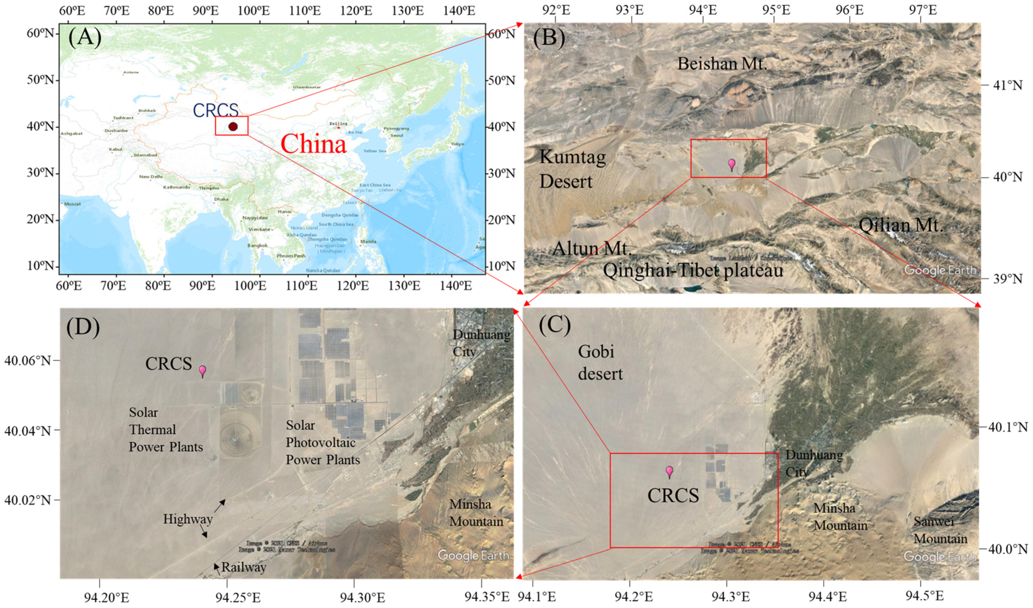
XCO2 and XCH4 were measured from June 26 to 19 July 2021, at the Chinese Radiometric Calibration Site (CRCS) (40.08° N, 94.40° E, ~1230 m a.s.l. (above sea level)), located in the Gobi Desert and approximately 20 km west of Dunhuang city in west China (Figure 1). There is no obvious emission sources and respiration of CO2 through vegetation nearby, as the CRCS is situated on a stable alluvial fan whose surface consists of cemented gravels, some black or gray stones, and sands without any vegetation [28]. There are also no obvious anthropogenic sources nearby except highway passes (~5 km east and ~7 km south) and some solar photovoltaic power stations in the east (~5 km) and south directions (~2 km) (Figure 1). Dunhuang is located at the westernmost end of the Hexi Corridor, an important transportation route of silk roads from Ancient China to the Western regions, Central Asia, and Europe. There is Sanwei Mountain in the east, Mingsha Mountain in the south, Kumtag Desert in the west connecting Lop Nur and Taklimakan Desert, and Gobi Desert in the north connecting Tianshan Mountain (Figure 1). The climate in the Dunhuang area is typical warm temperate arid zones with annual precipitation of 42.2 mm, annual evaporation of 2505 mm, and an annual average temperature of 9.9 °C (–30.5 °C~41.7 °C). The average temperature, relative humidity, pressure during the sampling period were 28.9 ± 2.0 °C, 23.1% ± 2.0%, 868.3 ± 2.1 hPa, respectively. There were approximately 15 h of sunshine during the observation period with sunrise, mid-noon, and sunset times of approximately 6:20, 13:45, and 21:10 CST (Chinese standard time, UTC + 08:00), respectively. The delay between solar noontime at Dunhuang and CST noontime is about 1 h and 45 min (1:45).
2.2. Instrument
A cavity ring-down spectrometer (CRDS; Model G2301, Picarro, Inc., Santa Clara, CA, USA) was used to measure atmospheric CO2 and CH4 mole fractions continuously. The air was collected from the inlet on the roof of the building at CRCS (~5 m above the ground) into the Picarro G2301 spectrometer which was placed in the room at 25 °C. Both CO2 and CH4 mole fractions were reported as atmospheric dry air fractions. The Picarro G2301 spectrometer was calibrated by the standard gas (traced to WMO CO2 X2007 and CH4 X2004A scale) obtained from China Meteorological Administration before and after the campaign. Furthermore, another working standard was used to check the drift at CRCS. Meanwhile, a WS500 Weather station (Lufft GmbH, Fellbach, Germany) was used to measure temperature, relative humidity, pressure, wind speed, and direction close to the sampling inlet on the roof of the building at CRCS.
A portable Fourier transform spectrometer (EM27/SUN, SN134, Bruker Optical GmbH, Ettlingen, Germany) was used to measure solar spectra at a resolution of 0.5 cm−1. CO2, CH4, O2, and H2O spectra were measured by an InGaAs (Indium Gallium Arsenide) detector between 5000 and 12,000 cm−1, while CO spectra were measured by an extended InGaAs detector below 5000 cm−1 [12]. The EM27/SUN was placed on an outdoor desk (~1 m above the ground) at the CRCS. The EM27/SUN was installed manually in the morning of the sunny days and moved back to the building in the later afternoon.
CO2 and CH4 mole fractions were continuously monitored by Picarro G2301 spectrometer from 15:00 on 26 June 2021 to 8:00 on 20 July 2021, as well as the meteorological parameters by the weather station. Because EM27/SUN requires manual operation and can only be observed on sunny days, there are 12 days (26 and 28 June, 7, 8, 11, 12, 14–19 July) observations of XCO2, XCH4, and XCO at CRCS.
2.3. Data Processing Methods
XCO2, XCH4, and XCO were retrieved by PROFFAST software from the EM27/SUN raw spectral data following previous studies [11,21,22,29]. The prior (.map) files (including temperature, pressure, density, gravity, CO2, CH4, H2O, CO prior values from the height of 0 to 70 km of the atmosphere with an interval of 1 km) and the intraday pressure change used for PROFFAST were acquired from the TCCON server and local measurement of Weather Station, respectively. The modulation efficiencies (ME, 0.9902), phase errors (PE, 0.0049), and calibration factors (1.00014517 for XCO2 and 0.99982628 for XCH4) of EM27/SUN were obtained from the Karlsruhe Institute of Technology (KIT) and applied in the retrieval process. ME and PE values for the EM27/SUN used in this study were higher than the ensemble mean of the EM27/SUN tested in KIT (ME = 0.98417 and 0.98430 and PE = −0.00061 and −0.00068) [11,30]. Calibration factors were close to the ideal value (1.0) and agreed well with other EM27/SUN Spectrometers [30]. Raw CO2 and CH4 data from the Picarro G2301 spectrometer and meteorological data from Weather Station were first averaged to hourly data and then calculated to daily average values following the method in Wei, et al. [31].
Bias-corrected level 2 XCO2 from OCO-2 (OCO2_L2_Lite_FP 10r) and OCO-3 satellites (OCO3_L2_Lite_FP 10r) were obtained from Goddard Earth Sciences Data and Information Services Center (disc.gsfc.nasa.gov) (accessed on 8 November 2021). Bias-corrected level 2 XCO2 (V02.98) and XCH4 (V02.96) from the GOSAT satellite were obtained from GOSAT Data Archive Service (GDAS, data2.gosat.nies.go.jp) (accessed on 10 September 2021). Level 2 XCO2, XCH4, and XCO from GOSAT-2 were obtained from GOSAT-2 Data Archive Service (https://prdct.gosat-2.nies.go.jp, accessed on 1 March 2022). Meanwhile, offline level 2 XCH4 from Sentinel-5P (S5-P) were acquired from the Sentinel-5P Pre-Operations Data Hub (s5phub.copernicus.eu/dhus) (accessed on 10 September 2021). XCO2 and XCH4 from OCO-2, OCO-3, and GOSAT were selected for comparison with ground observations using a box centered at the CRCS site that spanned 5° latitude and 10° longitude on the same day, while ground-based EM27/SUN observations were selected within 1 h of the transit time of each satellite [17]. A similar method was also applied to XCH4 from S5-P except the select box narrowed from 5° × 10° to 2° × 2° due to its large swath (2600 km) and high spatial resolution (7 × 7 km) [32,33].
3. Results and Discussion
3.1. Temporal Variation of CO2 and CH4 Mole Fractions
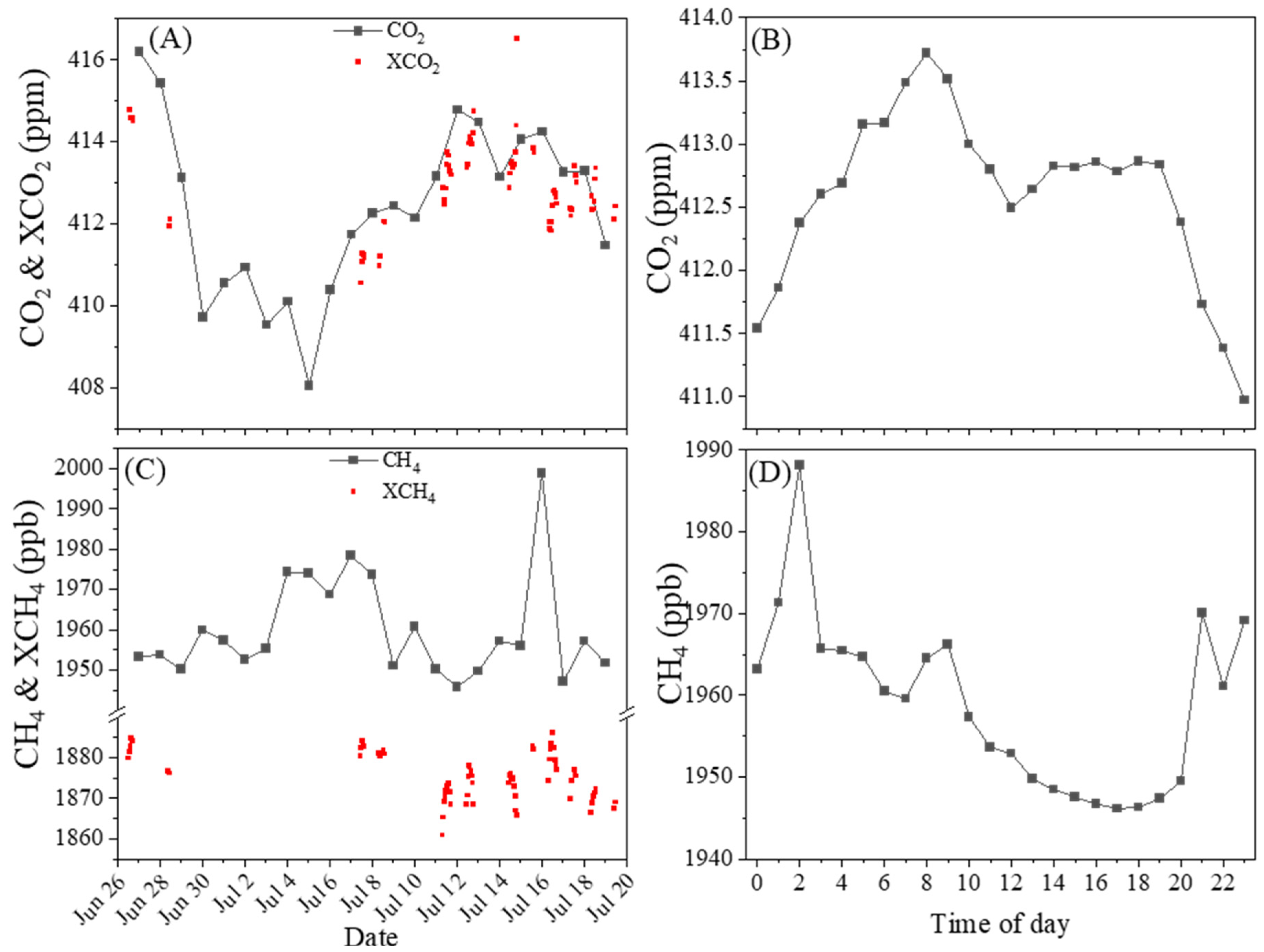
The average mole fractions of CO2 and CH4 at CRCS between 27 June and 19 July 2021 were 412.62 ± 2.06 ppm (average ± standard deviation) and 1959 ± 19 ppb, respectively (Table 1). Observations on 26 June and 20 July were excluded to calculate daily average values because the observation time was less than 18 h on the two days. These values are 5.93 ppm and 9 ppb higher than the monthly CO2 and CH4 mole fractions observed in July 2020 (406.69 ppm for CO2 and 1950 ppb for CH4, data accessed from the World Data Centre for Greenhouse gases (WDCGG)) at the Global background Waliguan Observatory, about 700 km southeast of CRCS. The CO2 mole fraction at CRCS was about 4.34 and 0.87 ppm lower than that observed at Mauna Loa Observatory and the global monthly average value in July 2021. Meanwhile, the CH4 mole fraction was 73 ppb higher than the global mean average value in July 2021 (monthly averaged CO2 and CH4 mole fractions were obtained from https://gml.noaa.gov/ccgg/trends/data.html, accessed on 27 March 2022).
In-situ observations provide a clear diel variation of GHGs because they can measure GHGs continuously in both daytime and nighttime. Diurnal CO2 and CH4 patterns at CRCS appeared in different modes (Figure 2). The diurnal CO2 mole fraction showed an M-mode curve (Figure 2B), which was different from the unimodal curve observed at Megacity Shanghai [31] and the nearby global background observatory Waliguan [34]. The CO2 mole fraction generally increased to the daily maximum value at 8:00 CST (Figure 2B) due to the accumulation of CO2 and the decrease in the PBL height. The CO2 mole fraction decreased to a trough at noon along with the increase in PBL height and photosynthesis effect after sunrise. However, the CO2 mole fraction stopped falling and rebounded to ~412.80 ppm until 19:00 and then decreased again to the daily lowest value at 23:00 (Figure 2B). One probable reason is that the vegetation in nearby desert oases (e.g., Dunhuang city in the east of CRCS) (Figure 1B,C) reduces their respiration and photosynthesis rate to adapt to high temperatures (>30 °C) [35] after 12:00 (Figure S1). Another possible reason is the influence of valley winds caused by the difference in the diurnal variation in the temperature between the basin and the mountain (Figure 1) [36]. The airmass with higher CO2 mole fractions from Dunhuang city passed by CRCS, and therefore, a constant CO2 mole fraction was monitored in the afternoon at a wind speed of ~1.5 m s−1 (Figure 2 and Figure S1). However, the CO2 mole fraction decreased in the evening (19:00–23:00) due to the changed wind direction from the city (~50° direction) to the mountains (~200° direction) (Figure 2 and Figure S1). The diurnal CH4 pattern (Figure 2D) was different from CO2 but similar to the summer pattern observed at the nearby Waliguan observatory except for morning time [37]. CH4 mole fraction peaked at 2:00 with a value of 1988 ppb, probably due to some anthropogenic emissions nearby. The original data were checked, and some rapidly rising and falling CH4 peaks occurred in the morning (Figure S2). The CH4 mole fraction at 21:00 on 5 July was also high (2150 ppb) and introduced a high hourly average mole fraction (Figure 2D). At the same time, the wind speed and direction were 1.8 m s–1 and 309° suggesting the probable emissions from the northwest direction. Furthermore, solar thermal power plants with molten salt in the south (~2 km) (Figure 1) likely release emissions such as CO2 and CH4 during their operation and maintenance. Although the technical details of the solar power plants nearby were not known, it was well documented that the solar power plants (e.g., the technology of power tower, parabolic trough, and linear Fresnel lens) use some natural gas or diesel for their operation and maintenance or back-up [38,39,40,41,42]. The CH4 mole fraction peaked at 9:00 in the daytime and then decreased to a valley at 17:00 because of the increase in PBL height and chemical removal of CH4 with OH radical [31,43]. The CH4 mole fraction increased again in the late afternoon (after 18:00 CST) due to a decrease in the PBL height and photochemical reaction rate (Figure 2D).
Dust storms have different effects on the mole fraction of GHGs in the Gobi Desert. A dust storm occurred in the late afternoon on July 18 and lasted for several days. The ambient CO2 mole fraction suddenly decreased by 1.2 ppm from 413.7 ppm to 412.5 ppm when the dust storm arrived, while the CH4 mole fraction increased by 5 ppb from 1947 to 1952 ppb (Figure S3). After the dust storm occurred, the hourly CO2 mole fraction decreased continuously until 6:00 CST the next day. However, the CH4 mole fraction decreased slightly and remained at 1950 ppb over the next 24 h (Figure S3B).
3.2. Temporal Variation of XCO2 and XCH4
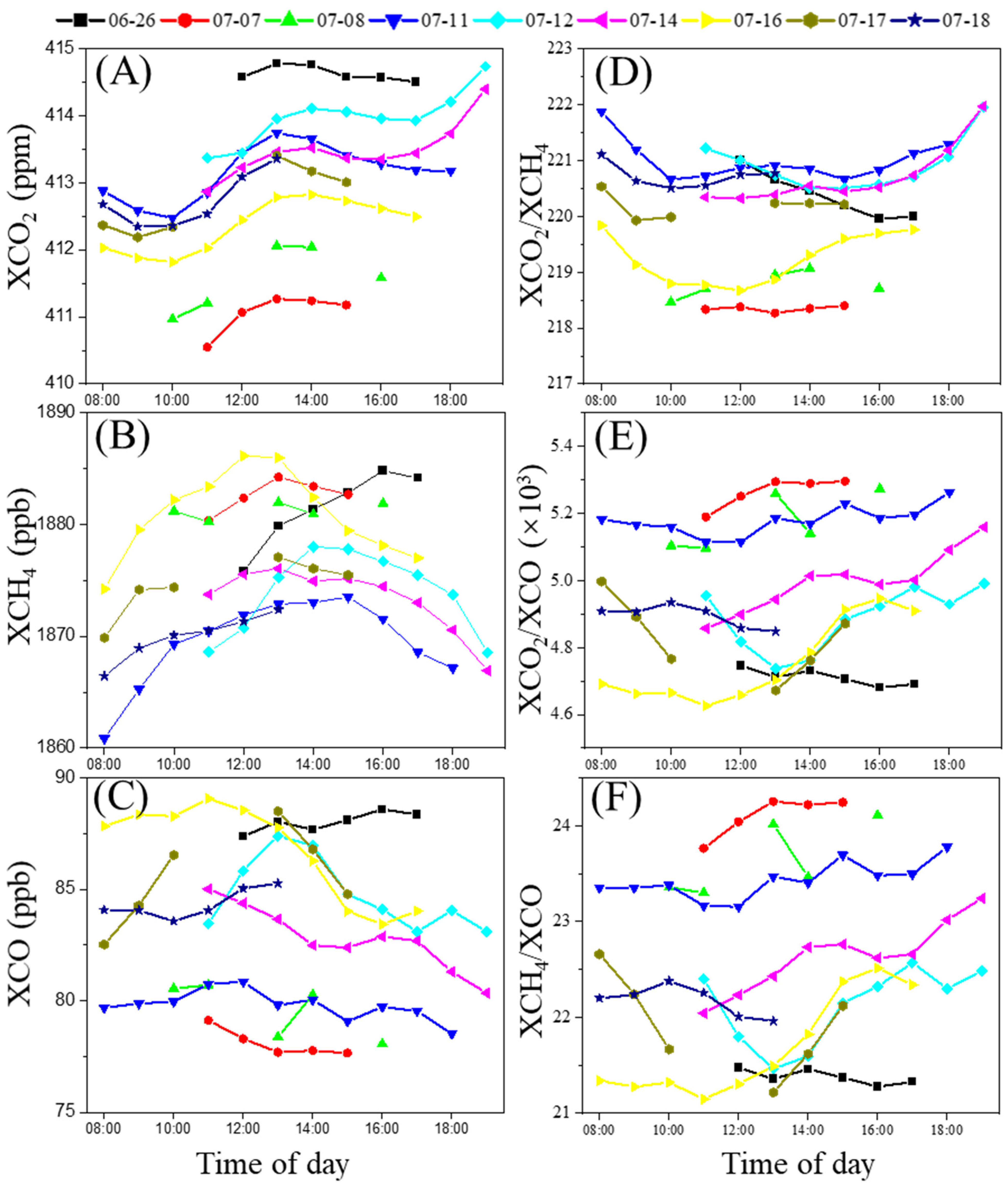
XCO2, XCH4, and XCO were averaged at 413.00 ± 1.09 ppm, 1876 ± 6 ppb, and 84 ± 3 ppb, respectively (Table 1). XCO2, XCH4, and XCO varied on different days and showed different diurnal patterns (Figure 3). The daily averaged XCO2 was highest on 26 June (414.63 ± 0.11 ppm) and decreased to 412.02 ppm on 28 June. XCO2 started to increase from the lowest value on 7 July (411.06 ± 0.30 ppm) to the second peak on 12 July (413.97 ± 0.40 ppm) and generally decreased thereafter (Figure 2, Table S1). Although XCO2 fluctuated on these days, the gap between the maximum and minimum daily average values was less than 1% (3.57 ppm). The PROFFAST software had already done airmass and independent airmass correction during the spectral processing process. The retrieved results may be affected by the potential airmass-dependent effects, because the XCO2 and XCH4 mole fractions were highest at noon and decreased along with an increase in solar zenith angle (SZA) (Figure S4) [10,44]. The daily averaged XCH4 remained at approximately 1880 ppb on the first four observed days but decreased to 1870 ppb on 11 July. XCH4 rebounded to a value >1880 ppb again on 15 July but decreased continuously thereafter to the lowest value on 19 July (1868 ± 1 ppb) (Figure 2, Table S1). Similar to XCO2, the concentration gap of maximum and minimum XCH4 values was also less than 1% (14 ppb). XCO was also high on 26 and 28 June, started to increase from 7 July to 15 July, and remained constant at around 85 ppb thereafter (Table S1). XCO2 was significantly correlated with CO2 (r = 0.51, p < 0.001), but XCH4 was not correlated with CH4 (r = 0.057, p = 0.645), suggesting the different behaviors of surface and column mole fractions of greenhouse gases, especially CH4. XCO was also significantly correlated with CO2 (r = 0.53, p < 0.001), and the correlation coefficient was higher than the coefficients between XCO and XCO2 (r = 0.33, p < 0.001) and XCH4 (r = 0.29, p < 0.001).
Both XCO2 and XCH4 showed diurnal variations. Diurnal variations of XCO2, XCH4, XCO, and their ratios on different days (observation time ≥5 h) are plotted together using the hourly average values (Figure 3). The observation time was not consistent on each day due to the differences in arrival and departure times at CRCS to set up EM27/SUN, as well as the weather conditions (e.g., enough sunshine). Diurnal XCO2 seemed to show sinusoidal mode curves (Figure 3A), similar to the observations (especially on 26 and 28 March 2008) at the Jet Propulsion Laboratory (JPL) in the South Coast Air Basin (SCB) of California, USA [45]. XCO2 decreased slightly from 8:00 to 10:00 (e.g., 11, 18, and 16 July) or 9:00 (17 July) in the morning, inversed after that to a noon peak at 13:00 or 14:00 (Solar noontime is ~13:45 at Dunhuang), and decreased again to the late afternoon continuously (26 June, 11, 26 July) or to an afternoon valley at 17:00 and reverse after that (12, 14 July). Sunshine and temperature could be the two factors that affected diurnal XCO2 variation in addition to anthropogenic emissions. After sunrise, plants in the surrounding oasis conduct photosynthesis and reduce the ambient XCO2 accumulated throughout the whole night. However, along with the rise of ambient temperature (which could exceed 30 °C at 11:00) (Figure S1), plants from nearby oases (Dunhuang city and nearby, Figure 1B,C) could close their stomata to reduce water evaporation and decrease their photosynthetic efficiency [35], resulting in an increase of XCO2 in the atmosphere. After noontime, XCO2 decreased again along with the decrease in anthropogenic activities (due to high temperature) and recovery of plant photosynthesis in the nearby oasis. The XCO2 increases again in the late afternoon due to the recovery of anthropogenic activities and the decrease in plant photosynthesis. The hourly XCH4 showed unimodal distributions in the daytime (e.g., 16, 12, 14, and 11 July), which were different from those of XCO2 (Figure 3B). XCH4 increased continuously in the morning due to biological and anthropogenic emissions from the surrounding area, especially from nearby Dunhuang city (20 km east). It is expected that the diurnal OH radical variation in Dunhuang is similar to that in other regions with the highest values around local noontime, such as in Beijing, Shanghai, and Pearl River Delta regions [46,47,48,49]. Thus, the XCH4 could increase in the morning due to the absence or lack of OH radicals. Along with the production of OH radicals under sunshine in the daytime, the increase in XCH4 slowed down and reversed at local noon (Figure 3B). Unlike XCO2 and XCH4, XCO did not show a significant diurnal variation, although its mole fraction decreased slightly in the afternoon (Figure 3C). The decreasing trend in the afternoon, especially on 12, 14, 16, and 18 July, is probably due to the removal of the reaction with OH radical [50]. XCO varied among 78–90 ppb (Figure 3C), which was about 30 ppb lower than that observed at Hefei city in eastern China [51]. Furthermore, the differences in the diurnal variations on most days were narrower than the differences among different days suggesting the emissions and the sinks of CO were relatively balanced at CRCS sites. XCO2/XCH4 were close to 221 on most days with lower ratios in the noontime but higher ratios in the morning and later afternoon (Figure 3D). Average XCO2/XCH4 (220 ± 1) was higher than the corresponding ratios of surface mole fractions of CO2 and CH4 (220 ± 1) (Table 1). XCO2/XCO and XCH4/XCO were averaged at 4.9 ± 0.2 (×103) and 22.5 ± 0.9 with small amplitude (Figure 3, Table 1). In general, hourly XCO2, XCH4, XCO, and their ratios show discrepancies on different days (Figure 3), mainly due to the changes in anthropogenic emissions and synoptic weather conditions [52].
3.3. Comparison between EM27/SUN and Satellite-Retrieved XCO2 and XCH4
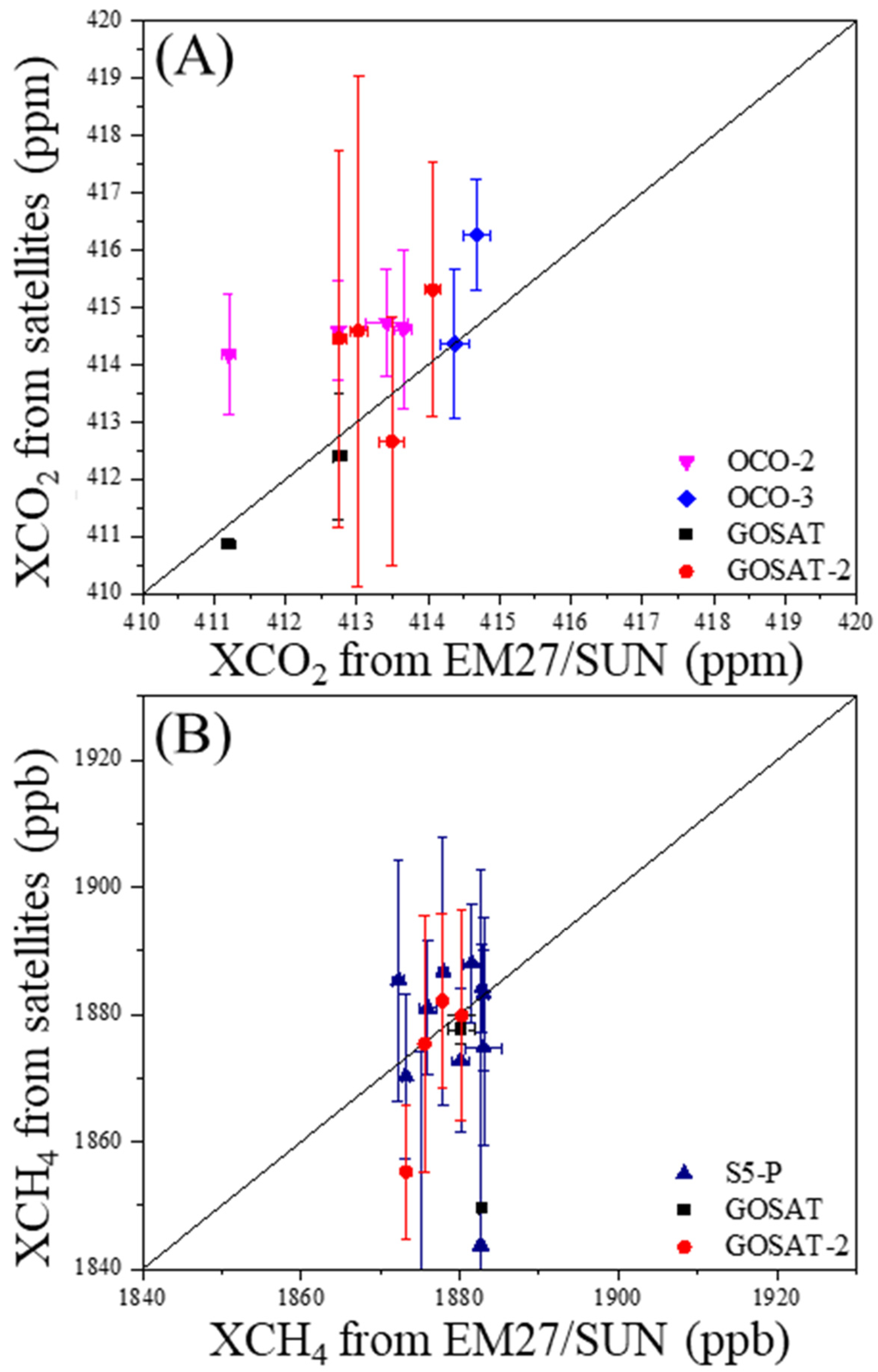
EM27/SUN observed XCO2 and XCH4 were compared with available satellite retrieves (Figure 4). Satellite retrieved XCO2 were obtained from GOSAT, GOSAT-2, OCO-2, and OCO-3, while XCH4 were acquired from GOSAT, GOSAT-2, and Sentinel-5 Precursor (S5-P). XCO2 from GOSAT was approximately 0.34 ppm (0.30–0.35 ppm) lower than those observed from EM27/SUN. XCO2 from GOSAT-2 were about 1.5 ppm (1.27–1.68 ppm) higher than the ground observations on 12, 16, and 17 July 2021, while on 11 July was −0.84 ppm lower than the ground observation (Table S3). XCO2 from OCO-3 were higher (1.59 ppm, 26 June) than or close to surface observations (0.001 ppm, 28 June). XCO2 from OCO-2 were all higher (1.77 ppm, 0.96–2.97 ppm) than ground-based observations (Figure 4A). XCH4 from GOSAT on July 16 (five observations) was 2.62 ppb lower than that from EM27/SUN, while XCH4 on 7 July (only 1 observation, 1850 ppb) was 33 ppb lower than the ground averaged value (Figure 4B). XCH4 from GOSAT-2 were mostly lower (−0.2~−18 ppb) than EM27/SUN observed values except on 11 July (4.5 ppb). Most XCH4 observations from S5-P and EM27/SUN fluctuated around the 1:1 line within 10 ppb, except 14 and 15 July with differences of 43 and 39 ppb, respectively (Figure 4B). The huge differences on 14 and 15 July were attributed to some footprints having very low XCH4 values (~300 ppb lower than the average values (~1900 ppb)) (Figure S5). In this case, the averaged XCH4 from S5-P was lower than the ground observed values (−0.32%, (satellite—EM27)/EM27), close to the systematic difference between S5-P bias-corrected XCH4 and TCCON data (−0.26%) [33]. XCO from GOSAT-2 was about 23 ppb (20–28 ppb) higher than the ground observations. The big differences in XCO observations might be originated from many factors and the most important of which is to confirm that the ground monitoring results are accurate in future work. The differences between different satellites and ground observations mainly originated from the differences in satellites payloads’ technologies (grating and Fourier transform spectrometers) and their field of views (FOVs) (continuous and discrete footprints at different sizes in the across-track direction), as well as the differences retrieved methods (full physics algorithm from different institutes) [9,53,54,55]. There are many studies validating satellite observations with ground observations at different locations, but the results were not the same. For example, Velazco, et al. [20] found GOSAT and OCO-2 XCO2 showed good consistency and the differences were 0.86 and 0.83 ppm after comparing with the TCCON Philippines site, while Mustafa, et al. [56] showed that GOSAT XCO2 was underestimated by 1.70 ppm while OCO-2 overestimated by 1.33 ppm after comparing with in-situ aircraft measurements in China. Liang, et al. [57] showed the standard deviation of GOSAT observations was larger than that of OCO-2 at TCCON sites. Velazco et al. [12] compared EM27/SUN observations of GOSAT M- and H-gain retrievals and the results reflected that H-gain retrievals were close to EM27 observations in desert Australia.
Most of the space- and ground-based observations are close to the 1:1 line with small differences (<0.1% for XCO2 and <0.6% for XCH4), indicating a good consistency of ground and satellite observations in the Gobi Desert region. Furthermore, the temporal differences of the ground-based observations within 2 h of the satellite’s transit were smaller than the spatial differences of satellite retrievals (Figure 4, Table S3), suggesting that spatially derived source-sink differences had a greater impact on the observed XCO2 and XCH4. The standard deviations (SD) for ground observed XCO2 within 1 h before and after the satellite transit time were ranged from 0.07 to 0.30 ppm, which was lower than those of satellite observations (0.87–4.46 ppm) within the coincidence criteria of 10° (longitude) × 5° (latitude) surrounding CRCS. The SDs of XCO2 from GOSAT-2 (2.18–4.46 ppm) were also higher than OCO-2, OCO-3, and GOSAT (0.87–1.38 ppm) (Table S3). The SDs for XCH4 from EM27/SUN observations (0.49–2.21 ppb) were also lower than satellites retrievals (2.30 ppb–58.88 ppb). Meanwhile, the average relative standard deviation (RSD) of EM27 observations was 0.03% (0.02%–0.07%) for XCO2 and 0.05% (0.03%–0.12%) for XCH4 (Table S3), suggesting the variations of XCO2 and XCH4 were very small, even less than the error of the equipment. The average RSD for satellite observations were 0.43% (0.21%–1.08%) for XCO2 and 0.95% (0.12%–3.19%) for XCH4 (Table S3). The differences between satellites and EM27/SUN observations ((satellite—EM27)/EM27) were 0.26% (−0.20%–0.72%) for XCO2 and −0.38% (−2.31%–0.70%) for XCH4. After deducting the influence of the two S5-P data (14 and 15 July, Figure S5), the difference of XCH4 would reduce to −0.13% (−1.77%–0.70%).
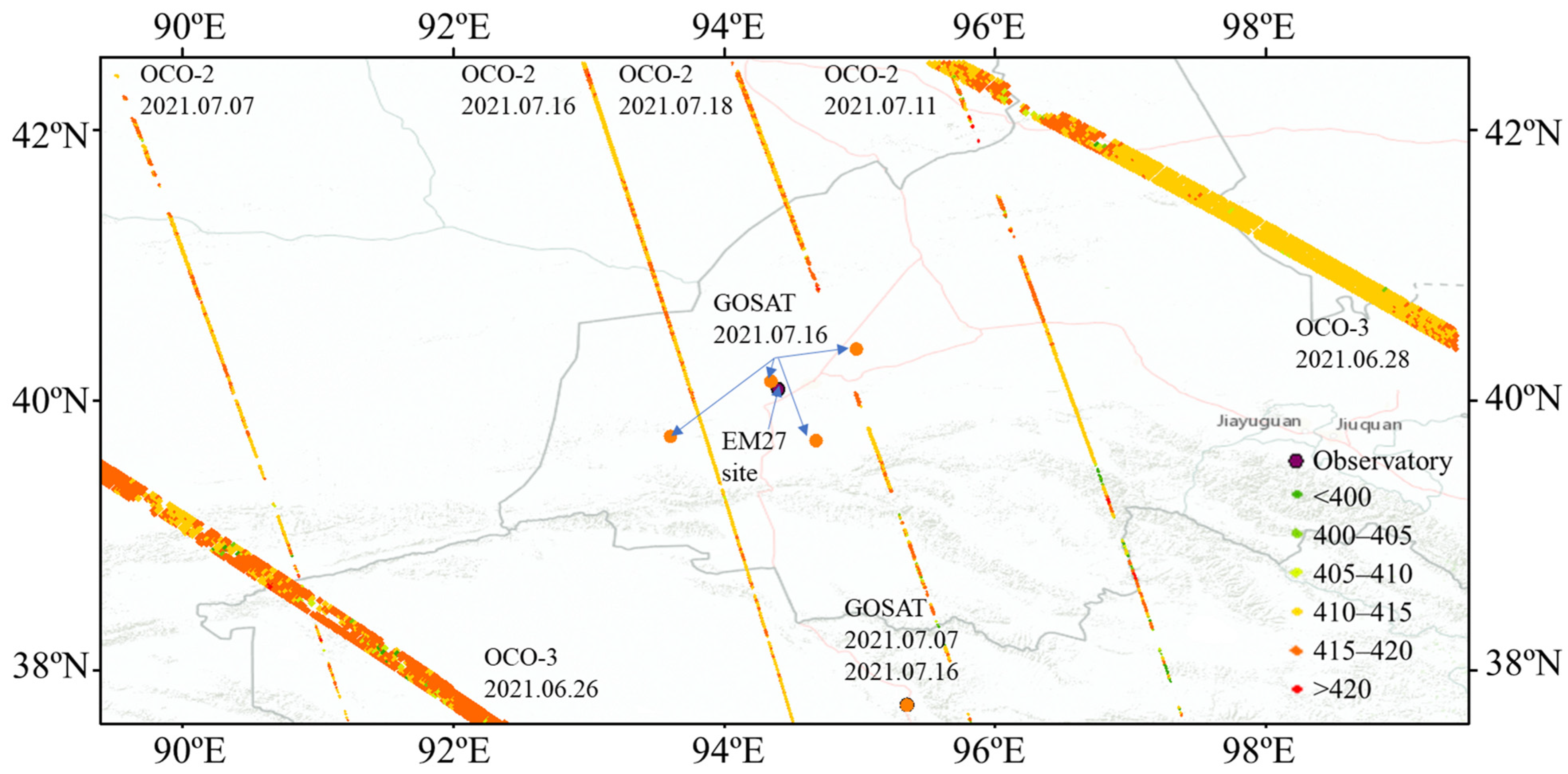
The satellites’ footprints were also plotted on the map to show the differences between ground and satellite XCO2 observations (Figure 5 and Figure S5). There was a footprint from GOSAT on 16 July close to the CRCS (Figure 5), XCO2 from GOSAT (411.75 ppm) was approximately 1 ppm lower than the surface observation (412.73 ppm), and XCH4 (1879.8 ppb) were close to EM27/SUN results (1880.7 ppb). This footprint was also observed by GOSAT-2 on 11, 16, and 17 July (Figure S6). XCO2 from GOSAT-2 on these days were 413.34, 416.00, and 411.63 ppm, respectively, which were higher (2.96 ppm on 17 July) or lower (−0.68 ppm on 11 July and −1.54 ppm on 16 July) than ground observations on the same time. Meanwhile, the differences of XCH4 among GOSAT-2 and ground observations (satellite minus surface observations) were less than 5 ppb (4.3, −3.2, and 3.4 ppb, respectively), while the differences in XCO varied bigger on different days (−3.1, 13.5, 1.48 ppb, respectively). The discrepancies between OCO-2/OCO-3 and ground EM27/SUN observations in the east of the CRCS were narrower than those in the west side. For example, the differences between OCO-2 and EM27/SUN on 11 and 18 July were 0.96 ppm and 1.31 ppm, which were narrower than the difference with the tracks in the west of CRCS on 7 July (2.97 ppm) and 16 July (1.86 ppm). Furthermore, the difference between OCO-3 and EM27/SUN in the east of the CRCS on 28 June was 0.001 ppm, which was also narrower than the OCO-3 track on the west side on 26 June (1.59 ppm). Fortunately, both GOSAT, GOSAT-2, and OCO-2 passed through the CRCS on 16 July, and the average XCO2 from OCO-2 (414.59 ± 0.87 ppm) was close to GOSAT-2 retrieved (414.45 ± 3.30 ppm), but higher than the results from GOSAT (412.40 ± 1.10 ppm) and EM27/SUN (412.74 ± 0.07 ppm).
3.4. Comparison with Surface In Situ and Column CO2 and CH4 Mole Fractions
The column mole fractions were also compared with in-situ observations at CRCS. Because ground EM27/SUN tracks the sun and observes its near-infrared spectrum to further retrieve XCO2 and XCH4, only GHGs in the daytime on cloudless days can be observed and retrieved. The XCO2 and XCH4 were 0.90 ppm and 72 ppb lower than their corresponding in situ CO2 and CH4 mole fractions observed at the same time, while their ratio was higher (Table 1). Hourly XCO2 was close to the daily and hourly averaged CO2 mole fractions on different days and showed similar trends (Figure 1A and Figure S2A). However, hourly XCH4 exhibited large gaps with CH4 mole fractions (Figure 1B and Figure S2B), probably due to photoreaction removal of CH4 in the upper atmosphere. The discrepancies of column and in-situ mole fractions were also reflected by the significant correlation between CO2 and XCO2 (r = 0.51, p < 0.01, n = 68) as well as XCO (r = 0.53, p < 0.01), but not for CH4 and XCH4 (r = 0.057, p = 0.645).
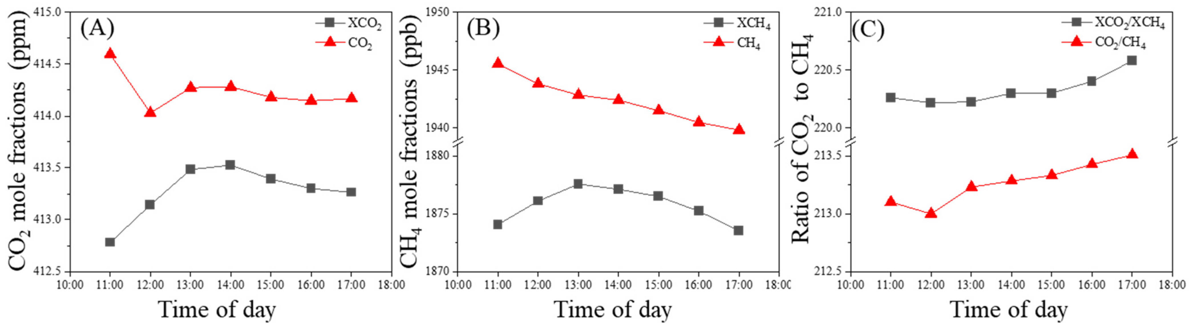
XCO2 and XCH4 showed different diurnal variation patterns with the corresponding CO2 and CH4 mole fractions (Figure 6). Hourly XCO2 and XCH4 (Figure 6) were calculated from the four days (11, 12, 14, and 16 July) because there were continuous observations in good weather conditions. Hourly XCO2 and XCH4 showed a curve like a dome from 11:00 to 17:00: their mole fractions started to increase in the morning and achieved their peak at 13:00 (XCH4) or 14:00 (XCO2), but XCH4 decreased faster than XCO2 because XCH4 at 17:00 was lower than that at 11:00 (Figure 6). The hourly averaged CO2 mole fraction in the four days decreased from 414.60 ppm at 11:00 to 414.03 ppm at 12:00 CST, and then showed a trend similar to that of XCO2 (Figure 6A). The gap between CO2 and XCO2 was lowest around the local mid-noon (0.76 ppm at 14:00 CST) but highest in the morning (1.82 ppm at 11:00 CST). Meanwhile, the hourly averaged CH4 mole fraction decreased monotonically from 11:00 to 17:00 CST due to photochemical removal and showed a similar trend to XCH4 after 13:00 (Figure 6B). The gap between CH4 and XCH4 was also largest at 11:00 (72 ppb), narrowed to ~65 ppb at 13:00, and remained there until 16:00. The mole fraction ratio of XCO2/XCH4 and CO2/CH4 exhibited a similar growth trend with a gap of approximately 7 (Figure 6C). Many factors could affect the diel mole fraction gaps between column and surface values. One probable reason might be the differences in sink processes because CO2 is mainly absorbed by ground vegetation, while CH4 can be removed by OH radical in the whole atmosphere. Another possible reason could be the influence of the changes in the planetary boundary layer (PBL) height. The PBL height could increase in the morning due to the heating effect of the ground after sunrise and thus dilute the near-surface GHG mole fractions under the PBL.
3.5. Influences of Meteorological Conditions
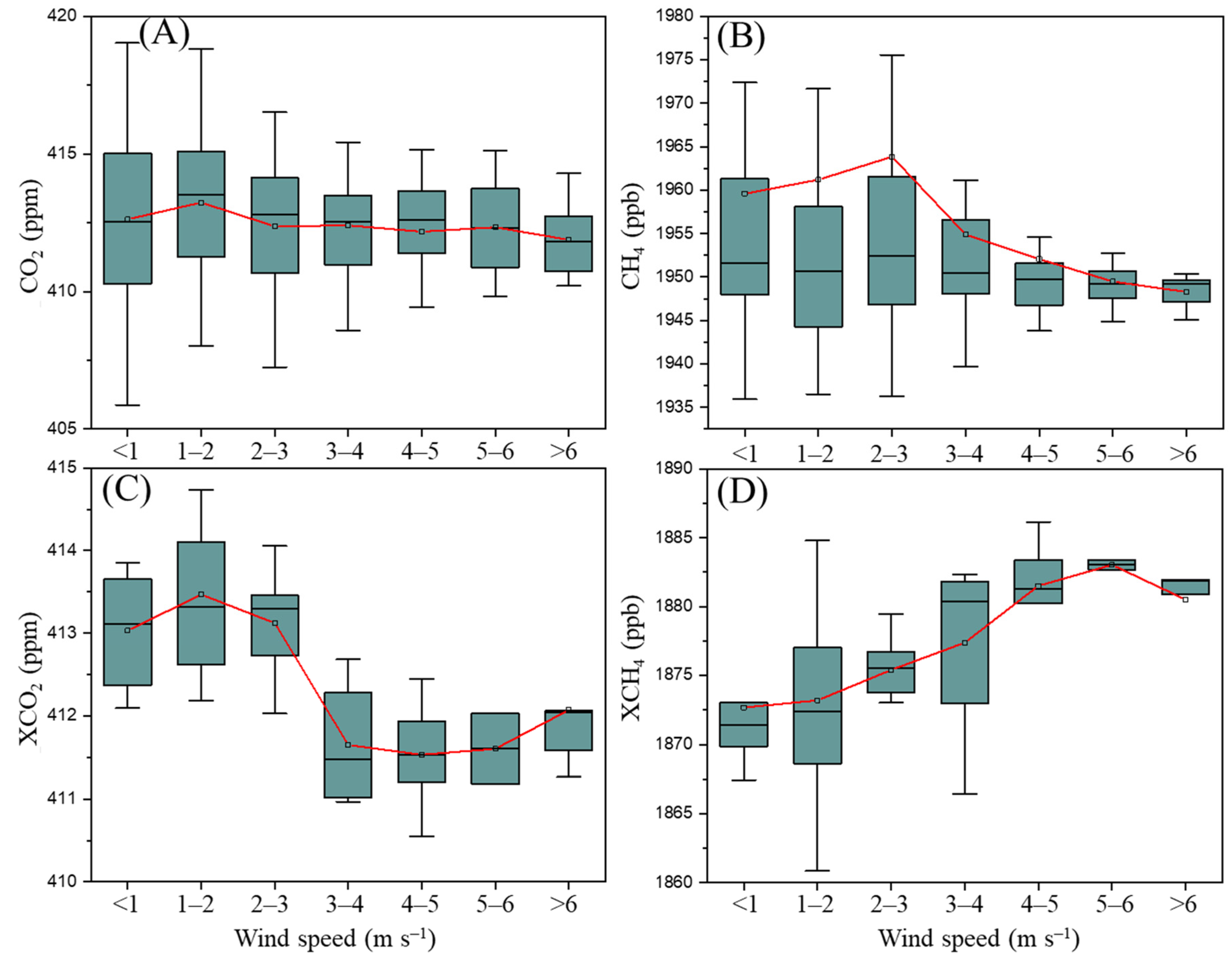
Wind could dilute a high concentration of atmospheric compositions from their source region and transport them to relatively clean areas. CO2 and CH4 mole fractions were 412.62 ± 2.94 ppm and 1960 ± 22 ppb at the wind speed at <1 m s−1, and increased to their highest values at wind speeds between 1 and 2 m s−1. Their mole fractions generally decreased with increasing wind speed (Figure 7A,B). The patterns were different from those observed in an urban site in Shanghai, where their mole fractions continuously decreased from the wind speed at <1 m s−1 to 3–4 m s−1 but reversed after that [31]. There are few emission sources around the observation site, so the mole fractions reflect the local background level near the CRCS under the lowest wind speed (<2 m s−1), and emissions from Dunhuang city were transported to the CRCS at higher wind speeds (2–4 m s−1), while clean airmasses from surrounding mountains were carried at the highest wind speed (>4 m s−1). Although XCO2 and XCH4 were column mole fractions, they also varied along with wind speed (Figure 7C,D). The XCO2 was highest (413.47 ppm) at 1–2 m s−1, and decreased to the lowest value (411.53 ppm) at 4–5 m s−1, but reversed at wind speeds >5 m s−1 (Figure 7C). However, the XCH4 increased continuously with increasing wind speed until 5 m s−1 (Figure 7D). GHG mole fractions and wind varied at different altitudes [16,58,59], which was probably the main reason for the discrepancy among surface and column mole fractions.
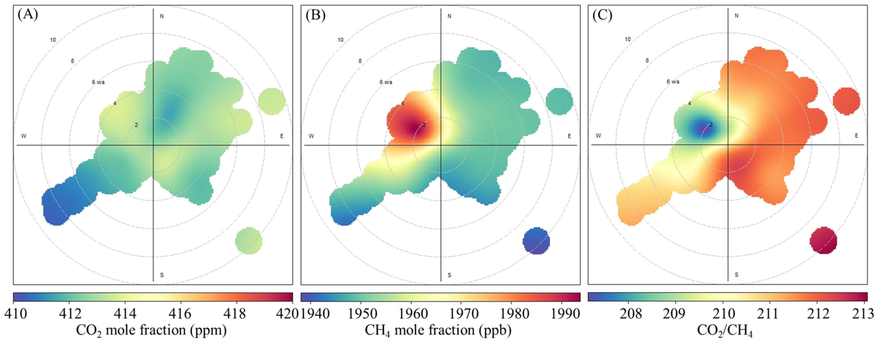
The bivariate polar plots provide a graphic method to show the impact of wind speed and wind direction on the concentrations of atmospheric compositions [31,60]. CO2 enhancements mainly occurred under the wind direction (WD) from the northeast and northwest, while its mole fractions can be diluted under the WD from the southwest (Figure 8A). Higher CH4 mole fraction mainly occurred under the WD from the northwest, similar to one of the CO2 source regions (Figure 8B), suggesting there was a point source from the northwest emitting both CO2 and CH4. The nearby solar thermal power plants (~2 km south of CRCS, Figure 1D) or other sources probably emitted some anthropogenic emissions and transport them to the CRCS. Wind from the southwest direction could bring the airmass with a lower CH4 mole fraction. The bivariate plot for XCO2 and XCH4 would be a useful tool to investigate the influences of wind in the future, although these plots cannot be drawn in this study due to the limited volume of hourly data.
4. Conclusions
XCO2 and XCH4 were first measured at a Gobi Desert site in western China in the summer of 2021. The diurnal XCO2 showed a sinusoidal model, while XCH4 appeared to have a unimodal distribution. Most of the satellite-retrieved XCO2 and XCH4 were close to the ground-observed values, but more differences appeared in the spatial distribution of satellite retrievals than the temporal change of ground observations. Ground-based XCO2 values were close to the surface CO2 mole fractions, while XCH4 had a large gap with CH4 mole fractions. Many factors could affect the temporal variation and discrepancy of column and surface CO2 and CH4 mole fractions, such as differences in sources and sinks, changes in PBL height, plant photosynthesis and respiration rate, chemical removal of CH4, valley wind, and dust storm. Wind can dilute and accumulate atmospheric CO2 and CH4 mole fractions from different wind directions, but its effect on XCO2 and XCH4 needs more investigation in the future because the wind also varies at different altitudes. The observation period in this study was short and some conclusions are not sufficient enough. A longer observation of column mole fractions, along with other atmospheric components, should be done in the future to obtain more valuable results and conclusions.
Supplementary Materials
The following supporting information can be downloaded at: https://0-www-mdpi-com.brum.beds.ac.uk/article/10.3390/atmos13040571/s1, Figure S1: Diurnal variation of temperature (A), relative humidity (B), pressure (C), wind speed (D), and wind direction (E) at Gobi desert site in Dunhuang, west China during the observation period (26 June to 19 July 2021), respectively; Figure S2: Variation of hourly CO2 (A) and CH4 (B) mole fractions (both surface and column) at Dunhuang from 26 June to 20 July, 2021; Figure S3: Variation of CO2 and CH4 mole fractions at the observation site before and after the dust storm in 2 h (A, data in 5 s average) and 1 day (B, hourly average data); Figure S4: Diurnal variations of XCO2, XCH4, and XCO and their variation with SZA (solar zenith angle) on 11 (A,B), 12 (C,D), 14 (E,F), and 16 (G,H) July 2021; Figure S5: Footprint of XCH4 mole fractions from S5-P over CRCS (2° × 2°) on 14 July and 15 July 2021; Figure S6: Footprints of XCO2 observations from GOSAT-2 near the EM27/SUN observation site from 26 June to 19 July; Table S1: The average mole fraction of XCO2, XCH4, and XCO as well as the observation hours and numbers during the observation period; Table S2: Comparison of the swath, footprint, spectrometer technologies, and data retrieved method of different satellites and the data version used in this study; Table S3: Comparison of satellite observed XCO2 and XCH4 with EM27/SUN observations. The coincidence criteria for OCO-2/OCO-3/GOSAT/GOSAT-2 was 10° × 5°, while for S5-P was 2° × 2° with a center of CRCS. EM27/SUN observations were averaged for ±1h of the satellite transit time.
Author Contributions
Conceptualization, L.B. and J.L.; methodology, C.W.; formal analysis, C.W.; investigation, C.W.; resources, Z.L., L.B. and J.L.; data curation, C.W.; writing—original draft preparation, C.W.; writing—review and editing, Z.L., L.B. and J.L.; visualization, C.W.; project administration, L.B. and J.L. All authors have read and agreed to the published version of the manuscript.
Funding
This research was jointly supported by the National Development and Reform Commission, China (18S-1926), the Shanghai Science and Technology Committee, China (21692195400), the Pudong New Area Science and Technology Development Fund (PKJ2021-C11), National Natural Science Foundation of China, China (41503119), the Shanghai Environmental Monitoring Center (HT2022162A1), and the International Partnership Program of Chinese Academy of Sciences (131211KYSB20180002).
Institutional Review Board Statement
Not applicable.
Informed Consent Statement
Not applicable.
Data Availability Statement
Satellite observed level 2 XCO2 from OCO-2 (version 10r) and OCO-3 (version 10r) were obtained from the Goddard Earth Sciences Data and Information Services Centre (disc.gsfc.nasa.gov, accessed on 10 January 2022). Satellite observed level 2 XCO2 (V02.98) and XCH4 (V02.96) from GOSAT were obtained from GOSAT Data Archive Service (data2.gosat.nies.go.jp, accessed on 10 January 2022). Satellite observed level 2 XCO2, XCH4 and XCO from GOSAT-2 were obtained from GOSAT-2 Data Archive Service (https://prdct.gosat-2.nies.go.jp, accessed on 1 March 2022). Offline level 2 XCH4 from Sentinel-5P (S5-P) were acquired from Sentinel-5P Pre-Operations Data Hub (s5phub.copernicus.eu/dhus, accessed on 10 January 2022). The EM27/SUN FTIR and G2301 spectrometer data at Dunhuang, China is available in the Science Data Bank (DOI: http://0-www-doi-org.brum.beds.ac.uk/10.11922/sciencedb.01233) (Wei and Lyu, 2021).
Acknowledgments
We thank Frank Hase and Qiansi Tu from Karlsruhe Institute of Technology (KIT), Germany for their support and guidance of PROFFAST.
Conflicts of Interest
The authors declare no conflict of interest.
References
- IPCC. Climate Change 2021: The Physical Science Basis. Contribution of Working Group I to the Sixth Assessment Report of the Intergovernmental Panel on Climate Change; Masson-Delmotte, V., Zhai, P., Pirani, A., Connors, S.L., Péan, C., Berger, S., Caud, N., Chen, Y., Goldfarb, L., Gomis, M.I., et al., Eds.; Cambridge University Press: Geneva, Switzerland, 2021. [Google Scholar]
- Friedlingstein, P.; O’Sullivan, M.; Jones, M.W.; Andrew, R.M.; Hauck, J.; Olsen, A.; Peters, G.P.; Peters, W.; Pongratz, J.; Sitch, S.; et al. Global Carbon Budget 2020. Earth Syst. Sci. Data 2020, 12, 3269–3340. [Google Scholar] [CrossRef]
- WMO. WMO Greenhouse Gas Bulletin (GHG Bulletin)—No.7: The State of Greenhouse Gases in the Atmosphere Based on Global Observations through 2011. 2012. Available online: https://library.wmo.int/doc_num.php?explnum_id=7276 (accessed on 27 March 2022).
- WMO. WMO Greenhouse Gas Bulletin (GHG Bulletin)—No.16: The State of Greenhouse Gases in the Atmosphere Based on Global Observations through 2019. 2020. Available online: https://library.wmo.int/doc_num.php?explnum_id=10437 (accessed on 27 March 2022).
- Saunois, M.; Stavert, A.R.; Poulter, B.; Bousquet, P.; Canadell, J.G.; Jackson, R.B.; Raymond, P.A.; Dlugokencky, E.J.; Houweling, S.; Patra, P.K.; et al. The Global Methane Budget 2000–2017. Earth Syst. Sci. Data 2020, 12, 1561–1623. [Google Scholar] [CrossRef]
- Dlugokencky, E. Trends in Atmospheruc Methane, NOAA/GML. Available online: https://gml.noaa.gov/ccgg/trends_ch4/ (accessed on 24 March 2022).
- Boesch, H.; Liu, Y.; Tamminen, J.; Yang, D.; Palmer, P.I.; Lindqvist, H.; Cai, Z.; Che, K.; Di Noia, A.; Feng, L.; et al. Monitoring Greenhouse Gases from Space. Remote Sens. 2021, 13, 2700. [Google Scholar] [CrossRef]
- Crisp, D.; Atlas, R.M.; Breon, F.M.; Brown, L.R.; Burrows, J.P.; Ciais, P.; Connor, B.J.; Doney, S.C.; Fung, I.Y.; Jacob, D.J.; et al. The Orbiting Carbon Observatory (OCO) mission. Adv. Space Res. 2004, 34, 700–709. [Google Scholar] [CrossRef] [Green Version]
- Crisp, D.; Meijer, Y.; Munro, R.; Bowman, K.; Chatterjee, A.; Baker, D.; Chevallier, F.; Nassar, R.; Palmer, P.I.; Agusti-Panareda, A.; et al. A Constellation Architecture for Monitoring Carbon Dioxide and Methane From Space. CEOS Atmospheric Composition Virtual Constellation Greenhouse Gas Team Report Version 1.2. 2018. Available online: https://ceos.org/document_management/Virtual_Constellations/ACC/Documents/CEOS_AC-VC_GHG_White_Paper_Publication_Draft2_20181111.pdf (accessed on 27 March 2022).
- Wunch, D.; Toon, G.C.; Blavier, J.-F.L.; Washenfelder, R.A.; Notholt, J.; Connor, B.J.; Griffith, D.W.T.; Sherlock, V.; Wennberg, P.O. The Total Carbon Column Observing Network. Philos. Trans. R. Soc. A Math. Phys. Eng. Sci. 2011, 369, 2087–2112. [Google Scholar] [CrossRef] [Green Version]
- Frey, M.; Sha, M.K.; Hase, F.; Kiel, M.; Blumenstock, T.; Harig, R.; Surawicz, G.; Deutscher, N.M.; Shiomi, K.; Franklin, J.E.; et al. Building the COllaborative Carbon Column Observing Network (COCCON): Long-term stability and ensemble performance of the EM27/SUN Fourier transform spectrometer. Atmos. Meas. Tech. 2019, 12, 1513–1530. [Google Scholar] [CrossRef] [Green Version]
- Velazco, V.A.; Deutscher, N.M.; Morino, I.; Uchino, O.; Bukosa, B.; Ajiro, M.; Kamei, A.; Jones, N.B.; Paton-Walsh, C.; Griffith, D.W.T. Satellite and ground-based measurements of XCO2 in a remote semiarid region of Australia. Earth Syst. Sci. Data 2019, 11, 935–946. [Google Scholar] [CrossRef] [Green Version]
- Keeling, C.D. The Concentration and Isotopic Abundances of Carbon Dioxide in the Atmosphere. Tellus 1960, 12, 200–203. [Google Scholar] [CrossRef] [Green Version]
- Keeling, C.D.; Bacastow, R.B.; Bainbridge, A.E.; Ekdahl, C.A., Jr.; Guenther, P.R.; Waterman, L.S.; Chin, J.F.S. Atmospheric carbon dioxide variations at Mauna Loa Observatory, Hawaii. Tellus 1976, 28, 538–551. [Google Scholar] [CrossRef] [Green Version]
- Shi, T.; Han, G.; Xin, M.; Gong, W.; Chen, W.; Liu, J.; Zhang, X.; Pei, Z.; Gou, H.; Bu, L. Quantifying CO2 Uptakes Over Oceans Using LIDAR: A Tentative Experiment in Bohai Bay. Geophys. Res. Lett. 2021, 48, e2020GL091160. [Google Scholar] [CrossRef]
- Zhang, Q.; Li, M.; Wei, C.; Mizzi, A.P.; Huang, Y.; Gu, Q. Assimilation of OCO-2 retrievals with WRF-Chem/DART: A case study for the Midwestern United States. Atmos. Environ. 2021, 246, 118106. [Google Scholar] [CrossRef]
- Wunch, D.; Wennberg, P.O.; Osterman, G.; Fisher, B.; Naylor, B.; Roehl, C.M.; O’Dell, C.; Mandrake, L.; Viatte, C.; Kiel, M.; et al. Comparisons of the Orbiting Carbon Observatory-2 (OCO-2) XCO2 measurements with TCCON. Atmos. Meas. Tech. 2017, 10, 2209–2238. [Google Scholar] [CrossRef] [Green Version]
- Wang, W.; Tian, Y.; Liu, C.; Sun, Y.; Liu, W.; Xie, P.; Liu, J.; Xu, J.; Morino, I.; Velazco, V.A.; et al. Investigating the performance of a greenhouse gas observatory in Hefei, China. Atmos. Meas. Tech. 2017, 10, 2627–2643. [Google Scholar] [CrossRef] [Green Version]
- Crisp, D.; Pollock, H.R.; Rosenberg, R.; Chapsky, L.; Lee, R.A.; Oyafuso, F.A.; Frankenberg, C.; O’Dell, C.W.; Bruegge, C.J.; Doran, G.B. The on-orbit performance of the Orbiting Carbon Observatory-2 (OCO-2) instrument and its radiometrically calibrated products. Atmos. Meas. Tech. 2017, 10, 59. [Google Scholar] [CrossRef] [Green Version]
- Velazco, V.; Morino, I.; Uchino, O.; Hori, A.; Kiel, M.; Bukosa, B.; Deutscher, N.; Sakai, T.; Nagai, T.; Bagtasa, G.; et al. TCCON Philippines: First Measurement Results, Satellite Data and Model Comparisons in Southeast Asia. Remote Sens. 2017, 9, 1228. [Google Scholar] [CrossRef] [Green Version]
- Gisi, M.; Hase, F.; Dohe, S.; Blumenstock, T.; Simon, A.; Keens, A. XCO2 measurements with a tabletop FTS using solar absorption spectroscopy. Atmos. Meas. Tech. 2012, 5, 2969–2980. [Google Scholar] [CrossRef] [Green Version]
- Hase, F.; Frey, M.; Blumenstock, T.; Groß, J.; Kiel, M.; Kohlhepp, R.; Mengistu Tsidu, G.; Schäfer, K.; Sha, M.K.; Orphal, J. Application of portable FTIR spectrometers for detecting greenhouse gas emissions of the major city Berlin. Atmos. Meas. Tech. 2015, 8, 3059–3068. [Google Scholar] [CrossRef] [Green Version]
- Knapp, M.; Kleinschek, R.; Hase, F.; Agustí-Panareda, A.; Inness, A.; Barré, J.; Landgraf, J.; Borsdorff, T.; Kinne, S.; Butz, A. Shipborne measurements of XCO2, XCH4, and XCO above the Pacific Ocean and comparison to CAMS atmospheric analyses and S5P/TROPOMI. Earth Syst. Sci. Data 2021, 13, 199–211. [Google Scholar] [CrossRef]
- Cai, Z.; Che, K.; Liu, Y.; Yang, D.; Liu, C.; Yue, X. Decreased Anthropogenic CO2 Emissions during the COVID-19 Pandemic Estimated from FTS and MAX-DOAS Measurements at Urban Beijing. Remote Sens. 2021, 13, 517. [Google Scholar] [CrossRef]
- CMA. Chinse Meteorological Administration: China Greenhouse Gases Bulletin. 2019. Available online: http://download.caixin.com/upload/2019zhongguo.pdf (accessed on 20 November 2021). (In Chinese).
- Yang, Y.; Zhou, M.; Langerock, B.; Sha, M.K.; Hermans, C.; Wang, T.; Ji, D.; Vigouroux, C.; Kumps, N.; Wang, G.; et al. New ground-based Fourier-transform near-infrared solar absorption measurements of XCO2, XCH4 and XCO at Xianghe, China. Earth Syst. Sci. Data 2020, 12, 1679–1696. [Google Scholar] [CrossRef]
- Schwandner, F.M.; Gunson, M.R.; Miller, C.E.; Carn, S.A.; Eldering, A.; Krings, T.; Verhulst, K.R.; Schimel, D.S.; Nguyen, H.M.; Crisp, D.; et al. Spaceborne detection of localized carbon dioxide sources. Science 2017, 358, eaam5782. [Google Scholar] [CrossRef] [Green Version]
- Hu, X.; Liu, J.; Sun, L.; Rong, Z.; Li, Y.; Zhang, Y.; Zheng, Z.; Wu, R.; Zhang, L.; Gu, X. Characterization of CRCS Dunhuang test site and vicarious calibration utilization for Fengyun (FY) series sensors. Can. J. Remote Sens. 2010, 36, 566–582. [Google Scholar] [CrossRef]
- Mermigkas, M.; Topaloglou, C.; Balis, D.; Koukouli, M.E.; Hase, F.; Dubravica, D.; Borsdorff, T.; Lorente, A. FTIR Measurements of Greenhouse Gases over Thessaloniki, Greece in the Framework of COCCON and Comparison with S5P/TROPOMI Observations. Remote Sens. 2021, 13, 3395. [Google Scholar] [CrossRef]
- Alberti, C.; Hase, F.; Frey, M.; Dubravica, D.; Blumenstock, T.; Dehn, A.; Surawicz, G.; Harig, R.; Orphal, J.; the EM27/SUN-partners team. Improved calibration procedures for the EM27/SUN spectrometers of the COllaborative Carbon Column Observing Network (COCCON). Atmos. Meas. Tech. Discuss. 2021, 2021, 1–48. [Google Scholar] [CrossRef]
- Wei, C.; Wang, M.; Fu, Q.; Dai, C.; Huang, R.; Bao, Q. Temporal characteristics of greenhouse gases (CO2 and CH4) in the megacity Shanghai, China: Association with air pollutants and meteorological conditions. Atmos. Res. 2020, 235, 104759. [Google Scholar] [CrossRef]
- Veefkind, J.P.; Aben, I.; McMullan, K.; Förster, H.; de Vries, J.; Otter, G.; Claas, J.; Eskes, H.J.; de Haan, J.F.; Kleipool, Q.; et al. TROPOMI on the ESA Sentinel-5 Precursor: A GMES mission for global observations of the atmospheric composition for climate, air quality and ozone layer applications. Remote Sens. Environ. 2012, 120, 70–83. [Google Scholar] [CrossRef]
- Sha, M.K.; Langerock, B.; Blavier, J.F.L.; Blumenstock, T.; Borsdorff, T.; Buschmann, M.; Dehn, A.; De Mazière, M.; Deutscher, N.M.; Feist, D.G.; et al. Validation of methane and carbon monoxide from Sentinel-5 Precursor using TCCON and NDACC-IRWG stations. Atmos. Meas. Tech. 2021, 14, 6249–6304. [Google Scholar] [CrossRef]
- Zhang, F.; Zhou, L.; Conway, T.J.; Tans, P.P.; Wang, Y. Short-term variations of atmospheric CO2 and dominant causes in summer and winter: Analysis of 14-year continuous observational data at Waliguan, China. Atmos. Environ. 2013, 77, 140–148. [Google Scholar] [CrossRef]
- Sharma, A.; Kumar, V.; Shahzad, B.; Ramakrishnan, M.; Singh Sidhu, G.P.; Bali, A.S.; Handa, N.; Kapoor, D.; Yadav, P.; Khanna, K.; et al. Photosynthetic Response of Plants under Different Abiotic Stresses: A Review. J. Plant Growth Regul. 2020, 39, 509–531. [Google Scholar] [CrossRef]
- Román-Cascón, C.; Yagüe, C.; Arrillaga, J.A.; Lothon, M.; Pardyjak, E.R.; Lohou, F.; Inclán, R.M.; Sastre, M.; Maqueda, G.; Derrien, S.; et al. Comparing mountain breezes and their impacts on CO2 mixing ratios at three contrasting areas. Atmos. Res. 2019, 221, 111–126. [Google Scholar] [CrossRef]
- Zhang, F.; Zhou, L.; Xu, L. Temporal variation of atmospheric CH4 and the potential source regions at Waliguan, China. Sci. China Earth Sci. 2013, 56, 727–736. [Google Scholar] [CrossRef]
- Suresh, C.; Saini, R.P. Review on solar thermal energy storage technologies and their geometrical configurations. Int. J. Energy Res. 2020, 44, 4163–4195. [Google Scholar] [CrossRef]
- Tian, Y.; Zhao, C.Y. A review of solar collectors and thermal energy storage in solar thermal applications. Appl. Energy 2013, 104, 538–553. [Google Scholar] [CrossRef] [Green Version]
- Li, R.; Zhang, H.; Wang, H.; Tu, Q.; Wang, X. Integrated hybrid life cycle assessment and contribution analysis for CO2 emission and energy consumption of a concentrated solar power plant in China. Energy 2019, 174, 310–322. [Google Scholar] [CrossRef]
- Behar, O.; Khellaf, A.; Mohammedi, K. A review of studies on central receiver solar thermal power plants. Renew. Sust. Energy Rev. 2013, 23, 12–39. [Google Scholar] [CrossRef]
- Lechón, Y.; de la Rúa, C.; Sáez, R. Life Cycle Environmental Impacts of Electricity Production by Solarthermal Power Plants in Spain. J. Sol. Energy Eng. 2008, 130, 021012. [Google Scholar] [CrossRef]
- Ghosh, A.; Patra, P.K.; Ishijima, K.; Umezawa, T.; Ito, A.; Etheridge, D.M.; Sugawara, S.; Kawamura, K.; Miller, J.B.; Dlugokencky, E.J.; et al. Variations in global methane sources and sinks during 1910–2010. Atmos. Chem. Phys. 2015, 15, 2595–2612. [Google Scholar] [CrossRef] [Green Version]
- Deutscher, N.M.; Griffith, D.W.T.; Bryant, G.W.; Wennberg, P.O.; Toon, G.C.; Washenfelder, R.A.; Keppel-Aleks, G.; Wunch, D.; Yavin, Y.; Allen, N.T.; et al. Total column CO2 measurements at Darwin, Australia—Site description and calibration against in situ aircraft profiles. Atmos. Meas. Tech. 2010, 3, 947–958. [Google Scholar] [CrossRef] [Green Version]
- Wunch, D.; Wennberg, P.O.; Toon, G.C.; Keppel-Aleks, G.; Yavin, Y.G. Emissions of greenhouse gases from a North American megacity. Geophys. Res. Lett. 2009, 36. [Google Scholar] [CrossRef] [Green Version]
- Nan, J.; Wang, S.; Guo, Y.; Xiang, Y.; Zhou, B. Study on the daytime OH radical and implication for its relationship with fine particles over megacity of Shanghai, China. Atmos. Environ. 2017, 154, 167–178. [Google Scholar] [CrossRef]
- Lu, K.; Guo, S.; Tan, Z.; Wang, H.; Shang, D.; Liu, Y.; Li, X.; Wu, Z.; Hu, M.; Zhang, Y. Exploring atmospheric free-radical chemistry in China: The self-cleansing capacity and the formation of secondary air pollution. Natl. Sci. Rev. 2018, 6, 579–594. [Google Scholar] [CrossRef] [Green Version]
- Lu, K.D.; Hofzumahaus, A.; Holland, F.; Bohn, B.; Brauers, T.; Fuchs, H.; Hu, M.; Häseler, R.; Kita, K.; Kondo, Y.; et al. Missing OH source in a suburban environment near Beijing: Observed and modelled OH and HO2 concentrations in summer 2006. Atmos. Chem. Phys. 2013, 13, 1057–1080. [Google Scholar] [CrossRef] [Green Version]
- Lu, K.D.; Rohrer, F.; Holland, F.; Fuchs, H.; Bohn, B.; Brauers, T.; Chang, C.C.; Häseler, R.; Hu, M.; Kita, K.; et al. Observation and modelling of OH and HO2 concentrations in the Pearl River Delta 2006: A missing OH source in a VOC rich atmosphere. Atmos. Chem. Phys. 2012, 12, 1541–1569. [Google Scholar] [CrossRef] [Green Version]
- Huang, Y.; Wei, J.; Jin, J.; Zhou, Z.; Gu, Q. CO Fluxes in Western Europe during 2017–2020 Winter Seasons Inverted by WRF-Chem/Data Assimilation Research Testbed with MOPITT Observations. Remote Sens. 2022, 14, 1133. [Google Scholar] [CrossRef]
- Shan, C.; Wang, W.; Liu, C.; Sun, Y.; Hu, Q.; Xu, X.; Tian, Y.; Zhang, H.; Morino, I.; Griffith, D.W.T.; et al. Regional CO emission estimated from ground-based remote sensing at Hefei site, China. Atmos. Res. 2019, 222, 25–35. [Google Scholar] [CrossRef] [Green Version]
- Vogel, F.R.; Frey, M.; Staufer, J.; Hase, F.; Broquet, G.; Xueref-Remy, I.; Chevallier, F.; Ciais, P.; Sha, M.K.; Chelin, P.; et al. XCO2 in an emission hot-spot region: The COCCON Paris campaign 2015. Atmos. Chem. Phys. 2019, 19, 3271–3285. [Google Scholar] [CrossRef] [Green Version]
- Yoshida, Y.; Kikuchi, N.; Morino, I.; Uchino, O.; Oshchepkov, S.; Bril, A.; Saeki, T.; Schutgens, N.; Toon, G.C.; Wunch, D.; et al. Improvement of the retrieval algorithm for GOSAT SWIR XCO2 and XCH4 and their validation using TCCON data. Atmos. Meas. Tech. 2013, 6, 1533–1547. [Google Scholar] [CrossRef]
- Lorente, A.; Borsdorff, T.; Butz, A.; Hasekamp, O.; aan de Brugh, J.; Schneider, A.; Wu, L.; Hase, F.; Kivi, R.; Wunch, D.; et al. Methane retrieved from TROPOMI: Improvement of the data product and validation of the first 2 years of measurements. Atmos. Meas. Tech. 2021, 14, 665–684. [Google Scholar] [CrossRef]
- Butz, A.; Hasekamp, O.P.; Frankenberg, C.; Vidot, J.; Aben, I. CH4 retrievals from space-based solar backscatter measurements: Performance evaluation against simulated aerosol and cirrus loaded scenes. J. Geophys. Res.-Atmos. 2010, 115. [Google Scholar] [CrossRef] [Green Version]
- Mustafa, F.; Wang, H.; Bu, L.; Wang, Q.; Shahzaman, M.; Bilal, M.; Zhou, M.; Iqbal, R.; Aslam, R.W.; Ali, M.A.; et al. Validation of GOSAT and OCO-2 against In Situ Aircraft Measurements and Comparison with CarbonTracker and GEOS-Chem over Qinhuangdao, China. Remote Sens. 2021, 13, 899. [Google Scholar] [CrossRef]
- Liang, A.; Gong, W.; Han, G.; Xiang, C. Comparison of Satellite-Observed XCO2 from GOSAT, OCO-2, and Ground-Based TCCON. Remote Sens. 2017, 9, 1033. [Google Scholar] [CrossRef] [Green Version]
- de Lange, A.; Landgraf, J. Methane profiles from GOSAT thermal infrared spectra. Atmos. Meas. Tech. 2018, 11, 3815–3828. [Google Scholar] [CrossRef] [Green Version]
- Bisht, J.S.H.; Machida, T.; Chandra, N.; Tsuboi, K.; Patra, P.K.; Umezawa, T.; Niwa, Y.; Sawa, Y.; Morimoto, S.; Nakazawa, T.; et al. Seasonal Variations of SF6, CO2, CH4, and N2O in the UT/LS Region due to Emissions, Transport, and Chemistry. J. Geophys. Res.-Atmos. 2021, 126, e2020JD033541. [Google Scholar] [CrossRef]
- Wei, C.; Wang, M.H.; Fu, Q.Y.; Dai, C.; Huang, R.; Bao, Q. Temporal characteristics and potential sources of black carbon in megacity Shanghai, China. J. Geophys. Res.-Atmos. 2020, 125, e2019JD031827. [Google Scholar] [CrossRef]
Figure 1.
Location of the CRCS observation site in the Gobi Desert in Dunhuang, western China. The subfigure (B–D) are the enlarged area in the red box of subfigures (A–C) respectively. The base map was obtained from Geoq, and the base figures were obtained from Google Earth, Image Landsat/Copernicus, Image 2021 © CNES/Airbus; Image © 2021 Maxar Technologies.

Figure 2.
Daily and hourly average mole fractions of surface CO2 (A,B) and CH4 (C,D), as well as hourly average column mole fractions of CO2 (A) and CH4 (C), observed at CRCS in Dunhuang, China.
Figure 2.
Daily and hourly average mole fractions of surface CO2 (A,B) and CH4 (C,D), as well as hourly average column mole fractions of CO2 (A) and CH4 (C), observed at CRCS in Dunhuang, China.

Figure 3.
Diurnal variation in EM27/SUN observed XCO2 (A), XCH4 (B), XCO (C), XCO2/XCH4 (D), XCO2/XCO (E), and XCH4/XCO (F) on different days. The format of the date is mm-dd on the top of the Figure.
Figure 3.
Diurnal variation in EM27/SUN observed XCO2 (A), XCH4 (B), XCO (C), XCO2/XCH4 (D), XCO2/XCO (E), and XCH4/XCO (F) on different days. The format of the date is mm-dd on the top of the Figure.

Figure 4.
Comparison of XCO2 (A) and XCH4 (B) observed from EM27/SUN and satellites (OCO-2, OCO-3, GOSAT, GOSAT-2, and S5-P) at CRCS in Dunhuang, western China.
Figure 4.
Comparison of XCO2 (A) and XCH4 (B) observed from EM27/SUN and satellites (OCO-2, OCO-3, GOSAT, GOSAT-2, and S5-P) at CRCS in Dunhuang, western China.

Figure 5.
Footprints of XCO2 observations from OCO-2, OCO-3, and GOSAT near the EM27/SUN observation site from 26 June to 19 July 2021. The observation data from different satellites were selected as a region spanning 5° latitude and 10° longitude of the center of the EM27/SUN site.
Figure 5.
Footprints of XCO2 observations from OCO-2, OCO-3, and GOSAT near the EM27/SUN observation site from 26 June to 19 July 2021. The observation data from different satellites were selected as a region spanning 5° latitude and 10° longitude of the center of the EM27/SUN site.

Figure 6.
Diurnal variation in hourly XCO2 (A) and XCH4 (B) mole fractions and their ratio (C), as well as the comparison with the corresponding greenhouse gas mole fractions and the ratio in the Gobi Desert in Dunhuang, China. The data were averaged from the hourly data on 11, 12, 14, and 16 July 2021.

Figure 7.
Boxplots of hourly average CO2 (A), CH4 (B), XCO2 (C), and XCH4 (D) mole fractions against wind speed. GHG mole fractions were binned by wind speed with an interval of 1 m s−1.
Figure 7.
Boxplots of hourly average CO2 (A), CH4 (B), XCO2 (C), and XCH4 (D) mole fractions against wind speed. GHG mole fractions were binned by wind speed with an interval of 1 m s−1.

Figure 8.
Bivariate polar plots for hourly CO2 and CH4 mole fraction and their ratio between 26 June and 19 July 2021 in Dunhuang, west China.
Figure 8.
Bivariate polar plots for hourly CO2 and CH4 mole fraction and their ratio between 26 June and 19 July 2021 in Dunhuang, west China.


Table 1.
Summary of surface and column mole fractions of greenhouse gases observed from 26 June to 19 July 2021, at a desert site in Dunhuang, west China.
Table 1.
Summary of surface and column mole fractions of greenhouse gases observed from 26 June to 19 July 2021, at a desert site in Dunhuang, west China.
| Unit | Mean | Min | Max | |
|---|---|---|---|---|
| Surface GHGs mole fraction a | ||||
| CO2 | ppm | 412.62 ± 2.06 | 408.30 | 416.44 |
| CH4 | ppb | 1959 ± 13 | 1945 | 1998 |
| CO2/CH4 | / | 211 ± 2 | 207 | 213 |
| Column GHGs and the corresponding surface GHGs mole fraction a | ||||
| XCO2 | ppm | 413.00 ± 1.09 | 410.55 | 416.51 |
| XCH4 | ppb | 1876 ± 6 | 1861 | 1886 |
| XCO | ppb | 84 ± 3 | 78 | 91 |
| XH2O | ppm | 3426 ± 749 | 1999 | 5175 |
| XCO2/XCH4 | / | 220 ± 1 | 218 | 223 |
| XCO2/XCO | ×10−3 | 4.9 ± 0.2 | 4.6 | 5.3 |
| XCH4/XCO | / | 22.5 ± 0.9 | 20.8 | 24.3 |
| CO2 b | ppm | 413.90 ± 1.80 | 409.99 | 419.97 |
| CH4 b | ppm | 1947 ± 11 | 1937 | 2015 |
| CO2/CH4 b | / | 213 ± 1 | 208 | 215 |
a, Surface mole fractions were calculated from daily average mole fractions from 27 June to 19 July 2021, while column mole fractions were calculated from hourly average values observed in the daytime. b, surface CO2, CH4 mole fraction, and their ratio were calculated from the hours with XCO2 values in this study.
Publisher’s Note: MDPI stays neutral with regard to jurisdictional claims in published maps and institutional affiliations. |
© 2022 by the authors. Licensee MDPI, Basel, Switzerland. This article is an open access article distributed under the terms and conditions of the Creative Commons Attribution (CC BY) license (https://creativecommons.org/licenses/by/4.0/).
Share and Cite
MDPI and ACS Style
Wei, C.; Lyu, Z.; Bu, L.; Liu, J. Occurrence and Discrepancy of Surface and Column Mole Fractions of CO2 and CH4 at a Desert Site in Dunhuang, Western China. Atmosphere 2022, 13, 571. https://0-doi-org.brum.beds.ac.uk/10.3390/atmos13040571
AMA Style
Wei C, Lyu Z, Bu L, Liu J. Occurrence and Discrepancy of Surface and Column Mole Fractions of CO2 and CH4 at a Desert Site in Dunhuang, Western China. Atmosphere. 2022; 13(4):571. https://0-doi-org.brum.beds.ac.uk/10.3390/atmos13040571
Chicago/Turabian StyleWei, Chong, Zheng Lyu, Lingbing Bu, and Jiqiao Liu. 2022. "Occurrence and Discrepancy of Surface and Column Mole Fractions of CO2 and CH4 at a Desert Site in Dunhuang, Western China" Atmosphere 13, no. 4: 571. https://0-doi-org.brum.beds.ac.uk/10.3390/atmos13040571
Note that from the first issue of 2016, this journal uses article numbers instead of page numbers. See further details here.