
Experimental Investigation of the Near-Surface Flow Dynamics in Downburst-like Impinging Jets Immersed in ABL-like Winds


Abstract
:1. Introduction
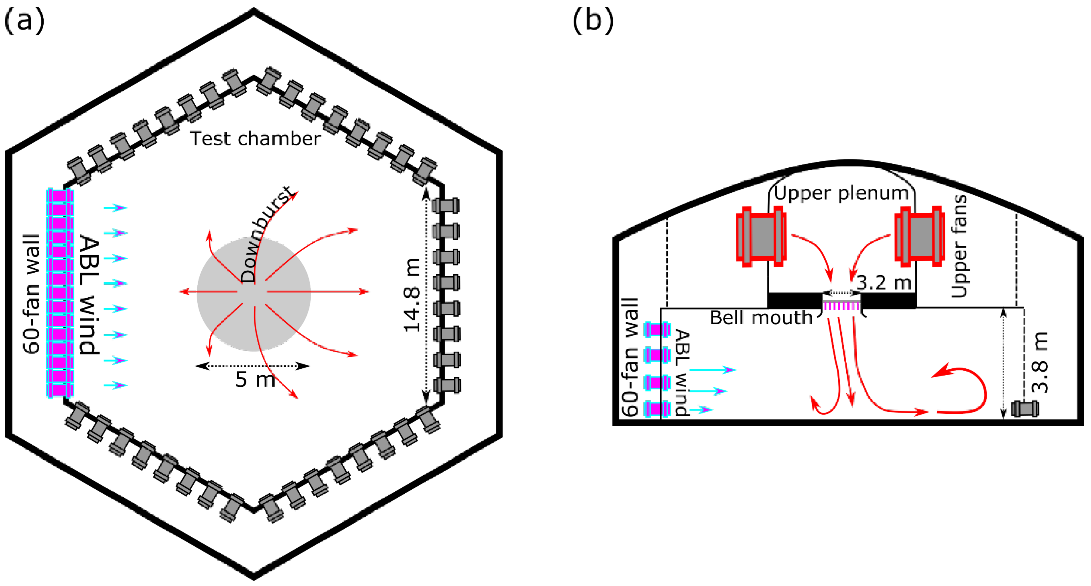
2. Experiment Setup
2.1. DB in ABL Mode and Flow Intensities
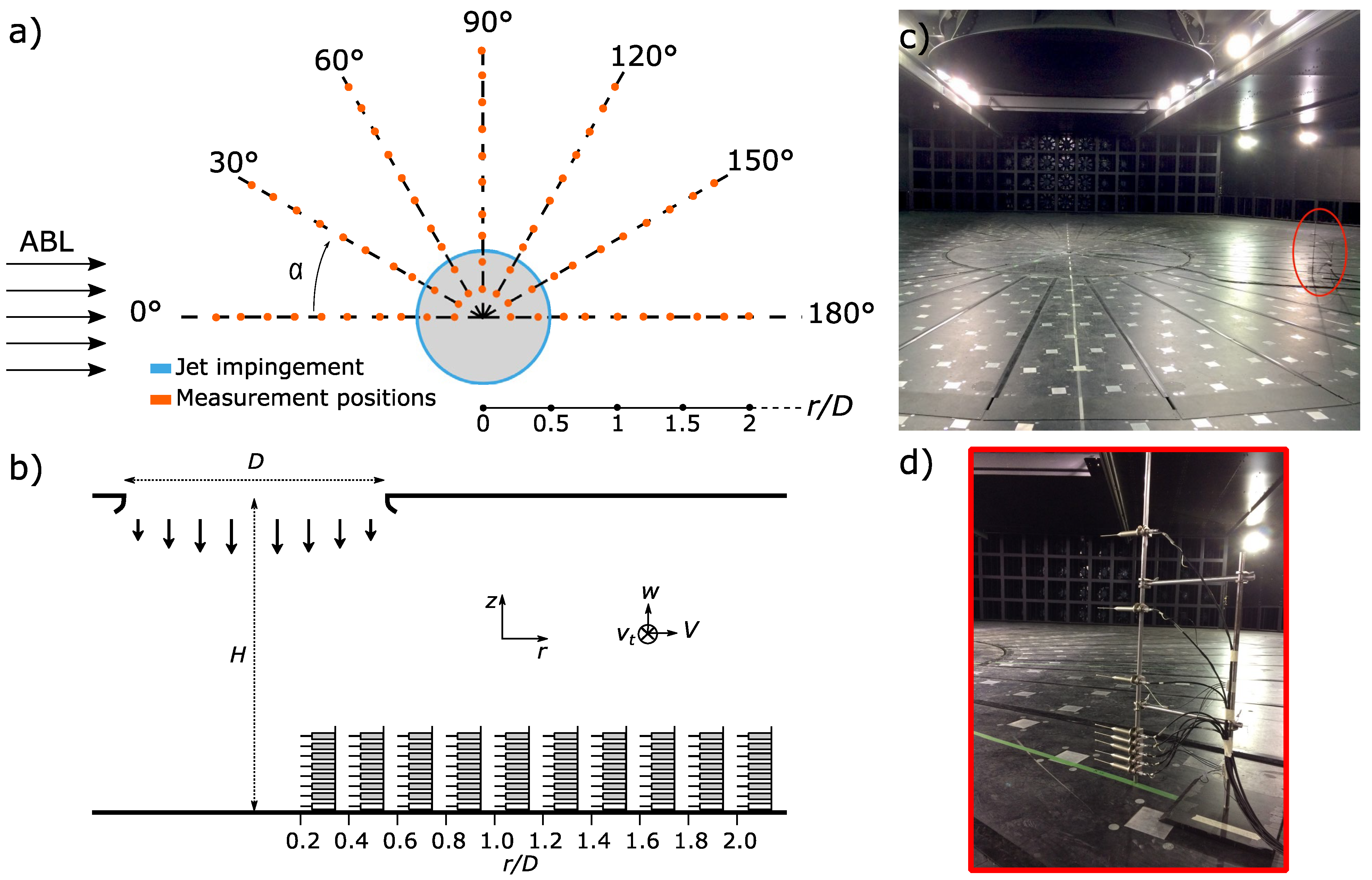
2.2. Cobra Probes Setup
2.3. ABL Vertical Profiles and DB–ABL Scaling Considerations
2.4. DB Vertical Profiles
3. Results and Discussion
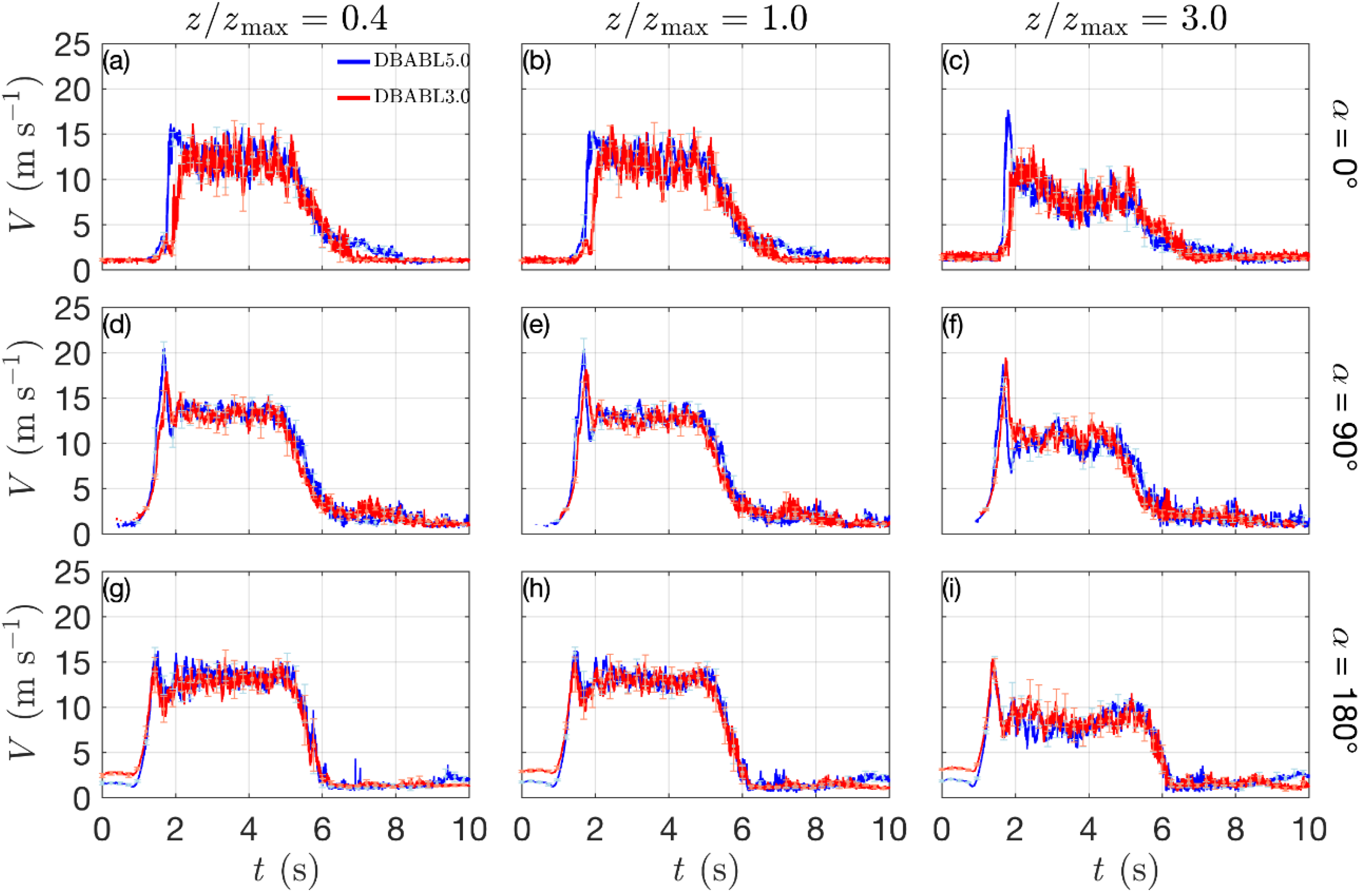
3.1. Wind Speed Time Histories
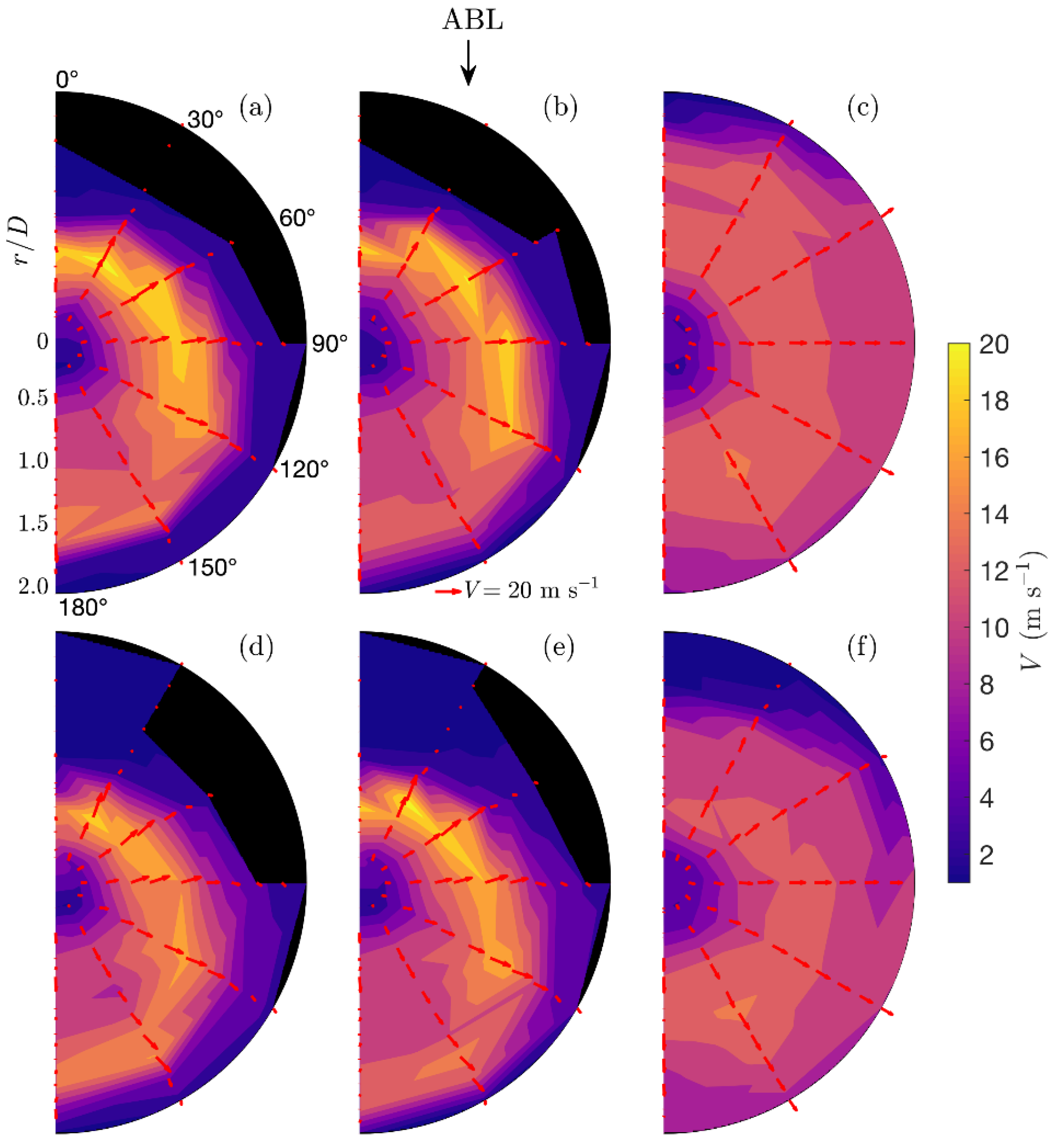
3.2. Spatial Reconstruction of the Wind Field
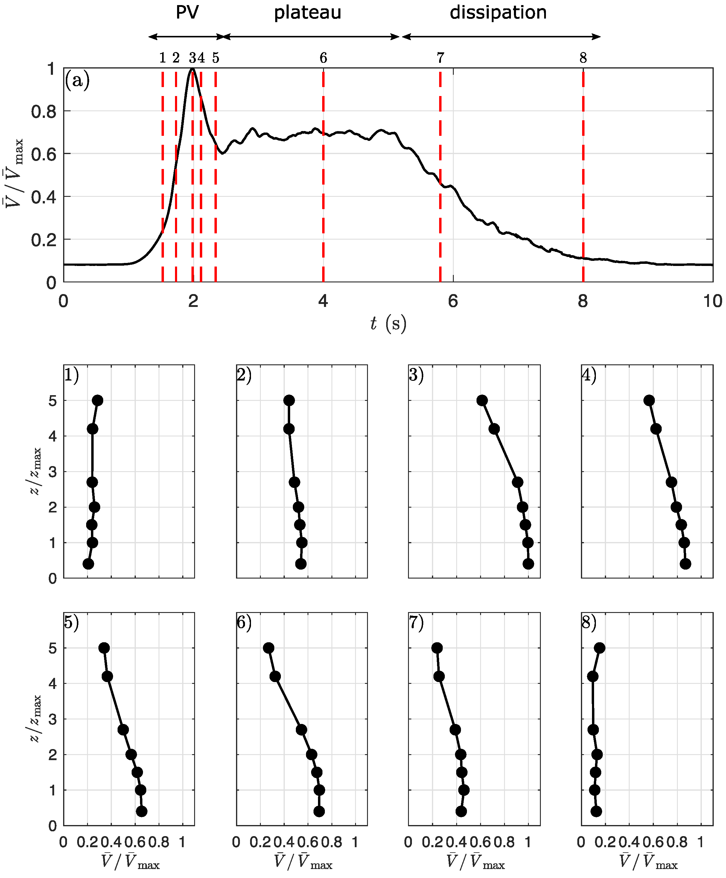
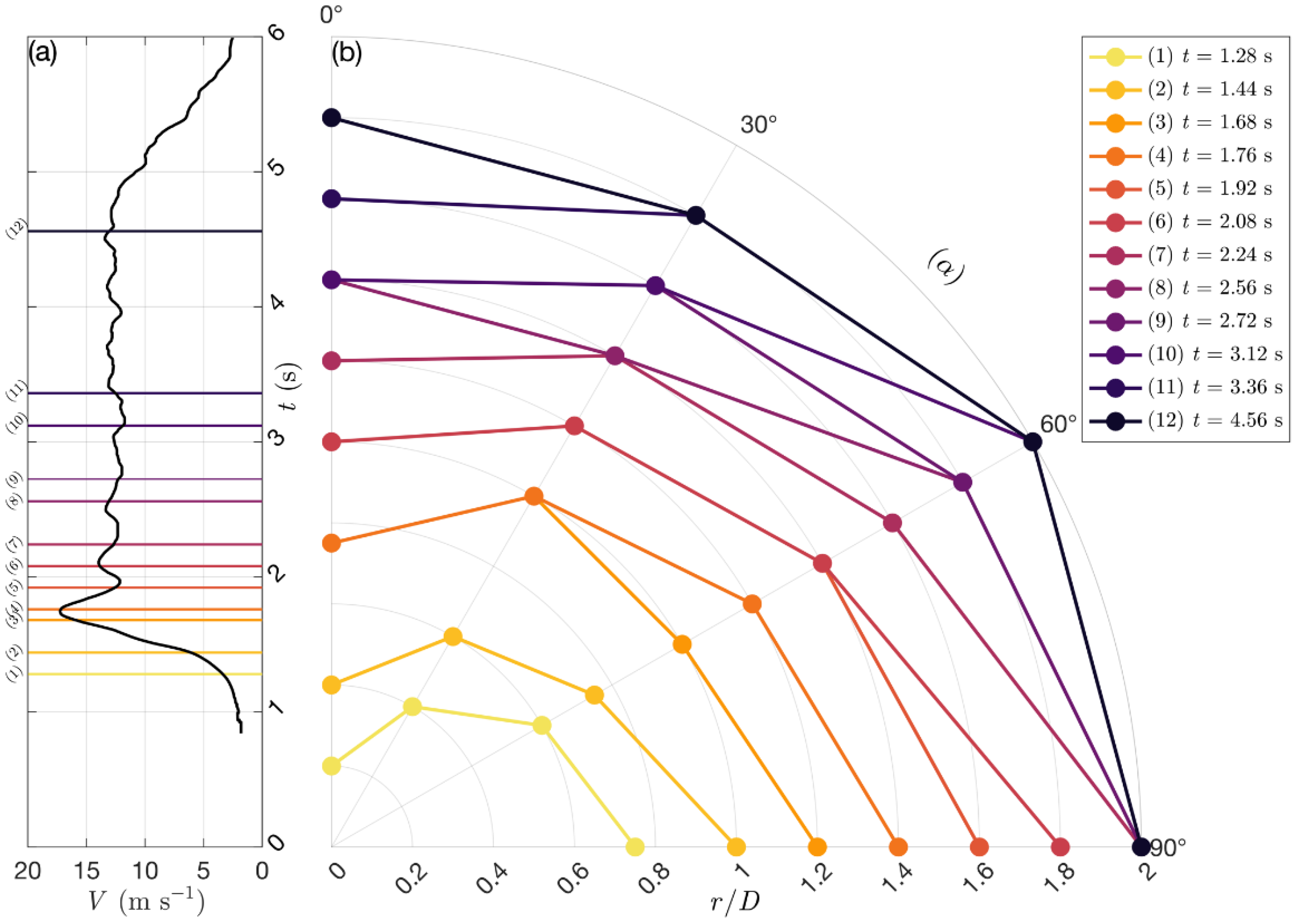
3.3. Gust Front Evolution
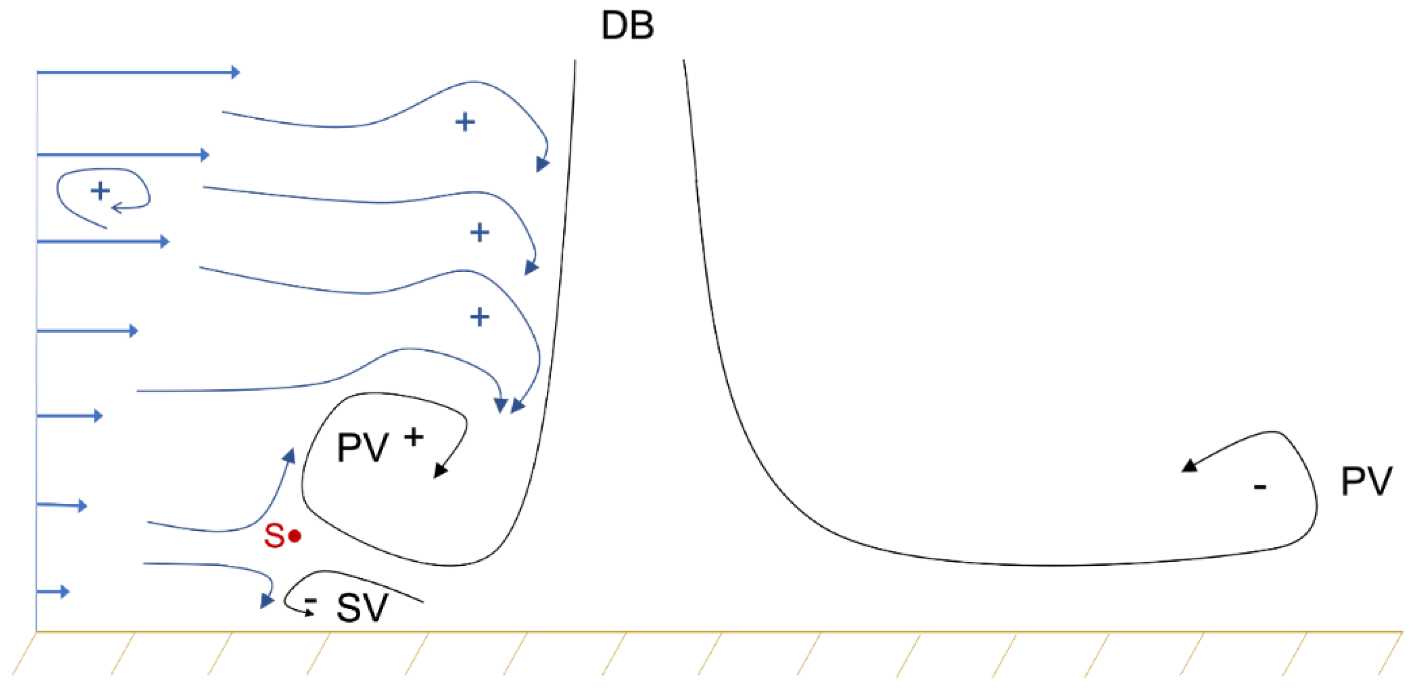
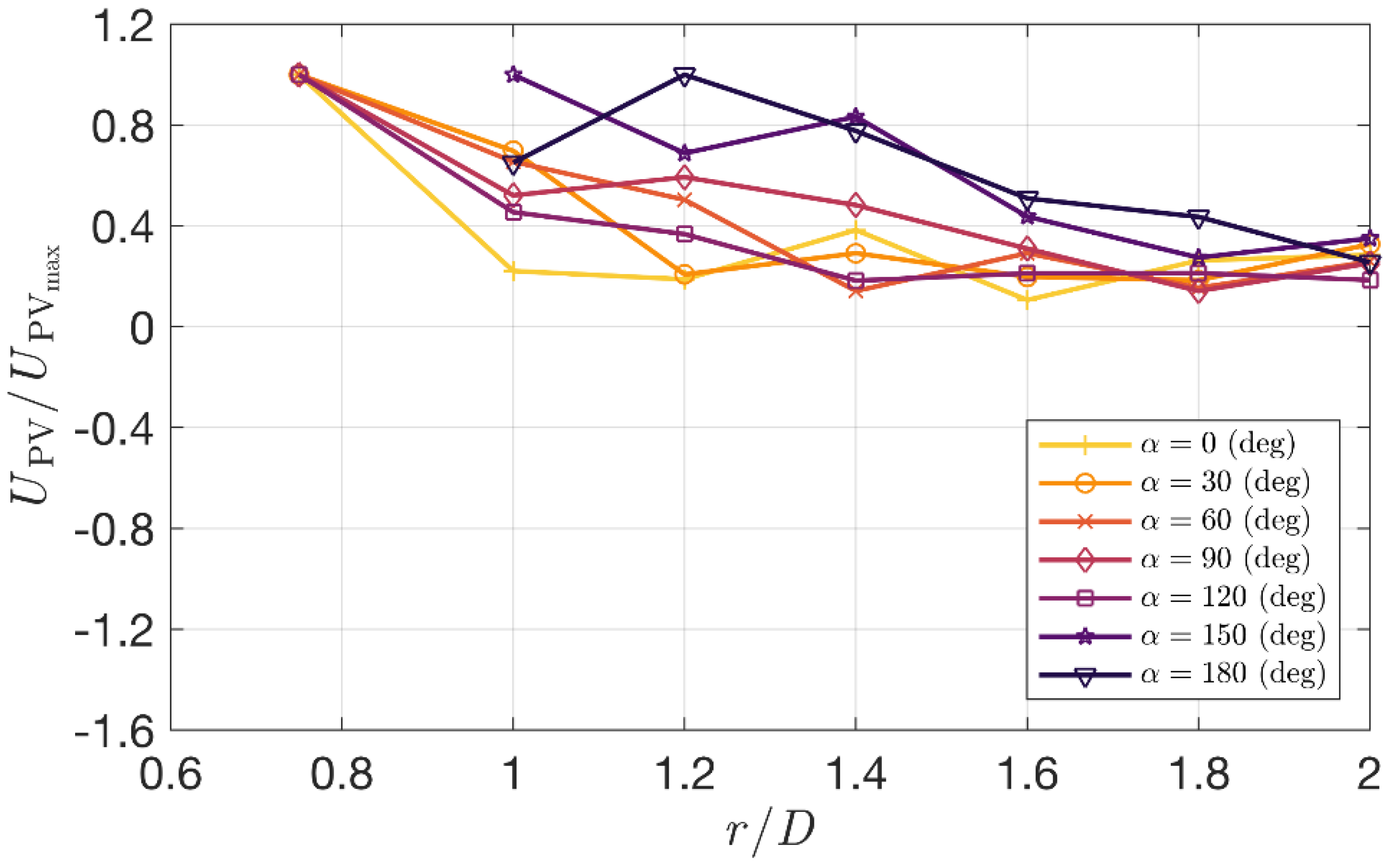
3.4. Primary Vortex Propagation
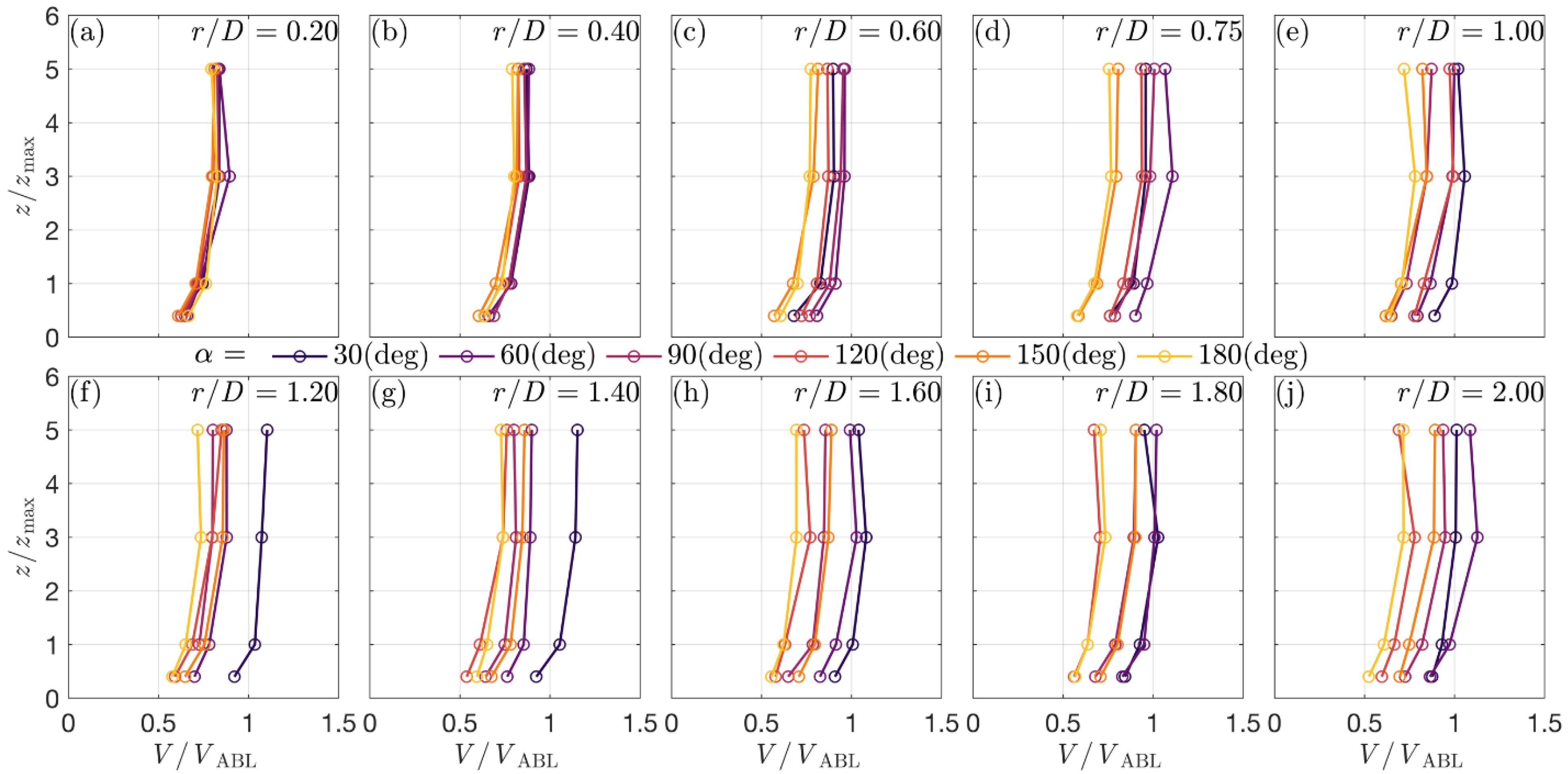
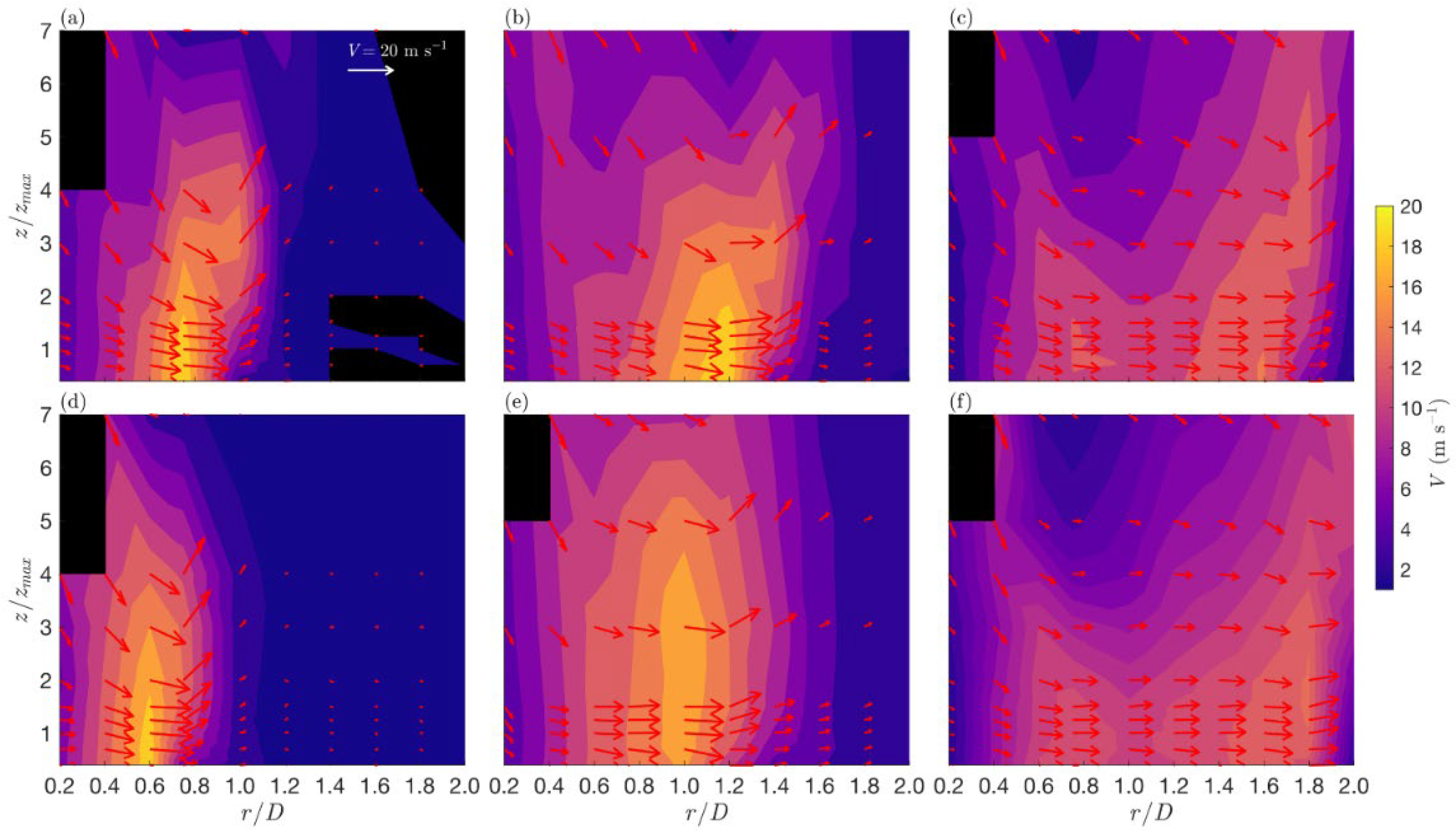
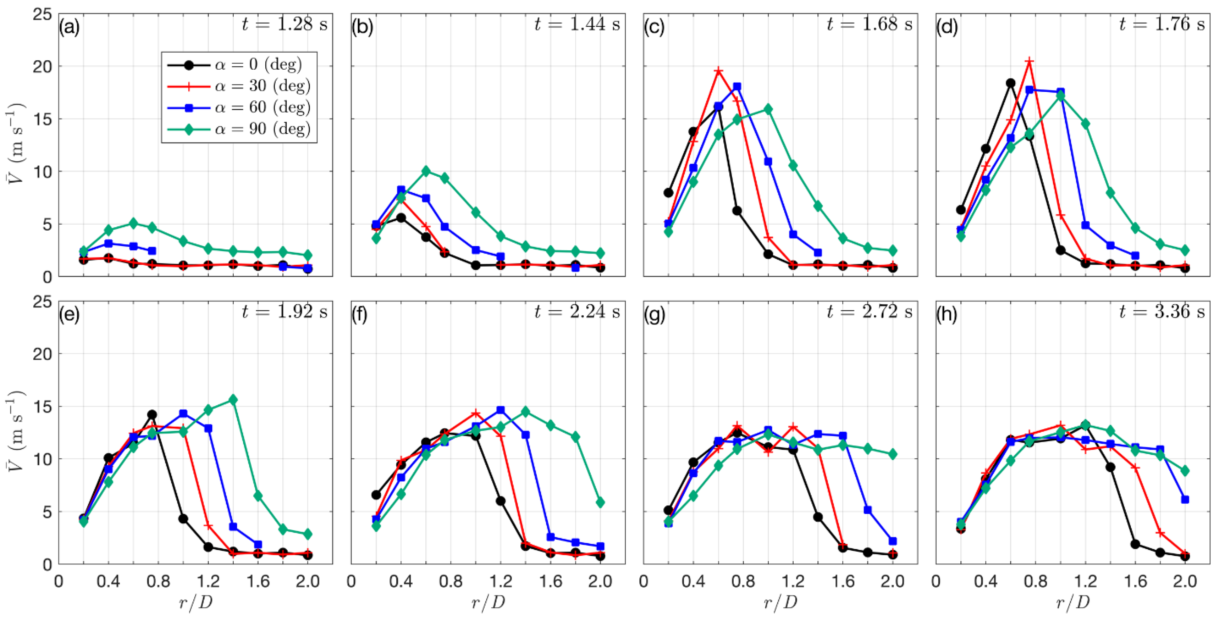
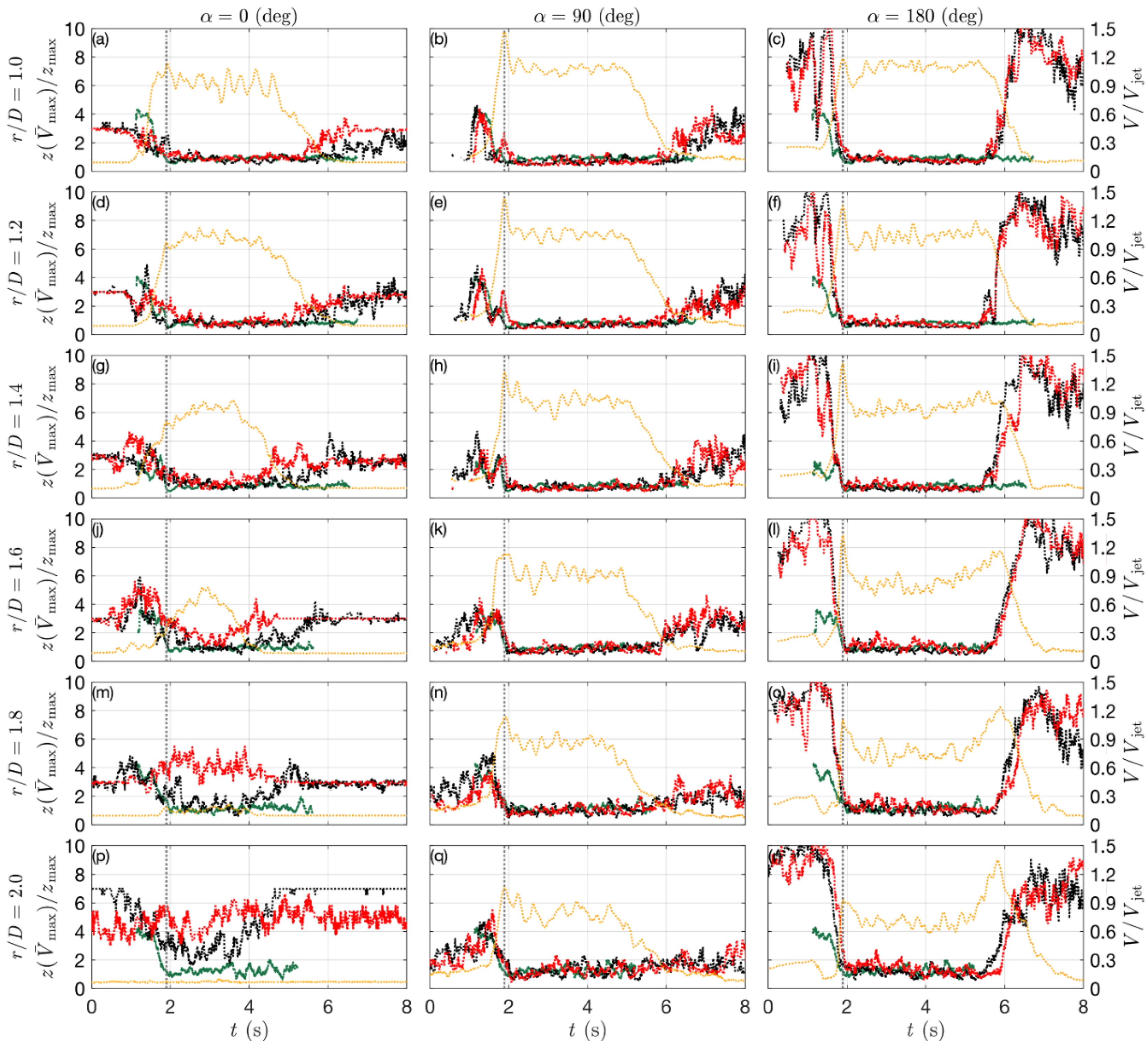
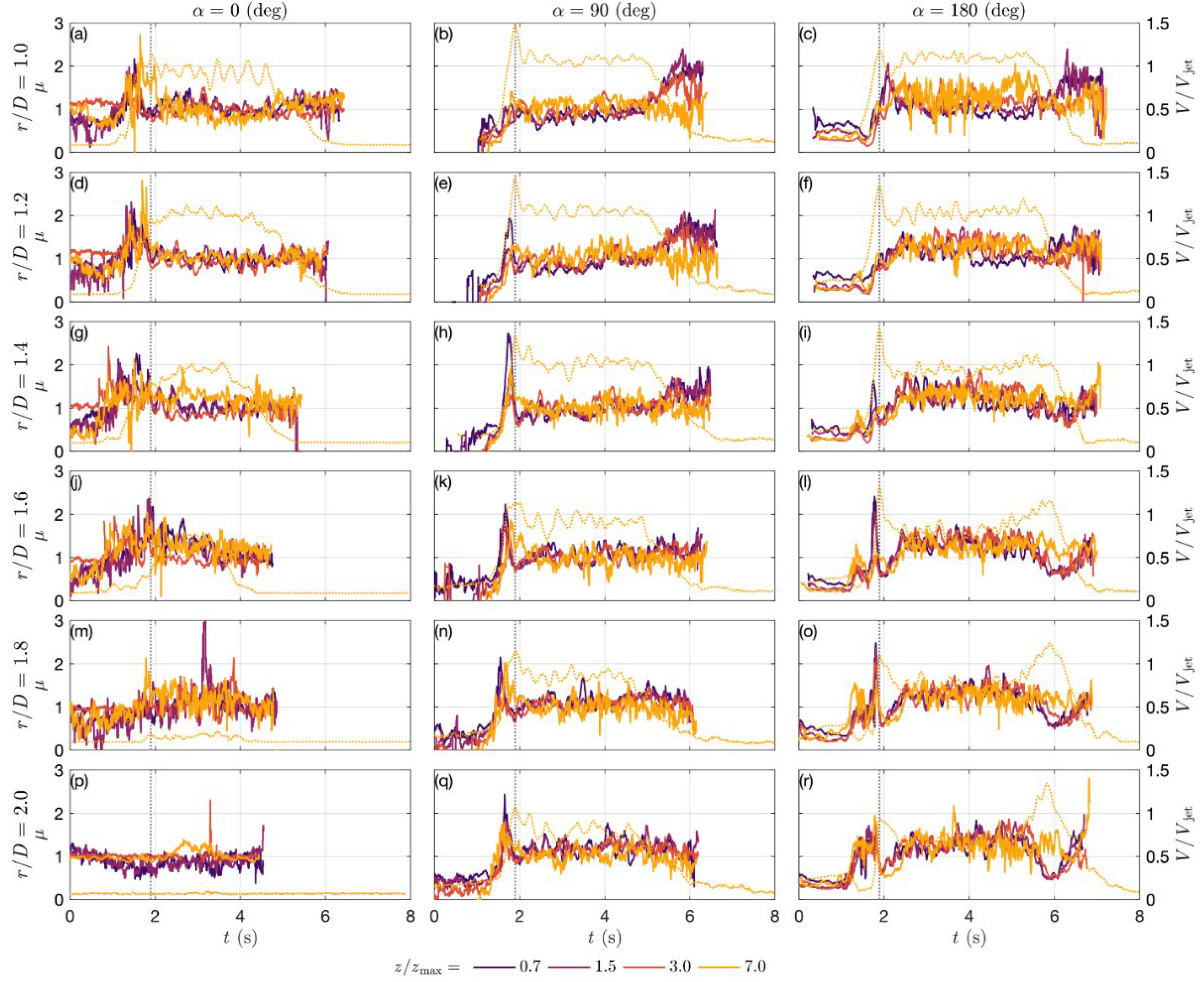
3.5. Vertical Profiles of Radial Wind Speed
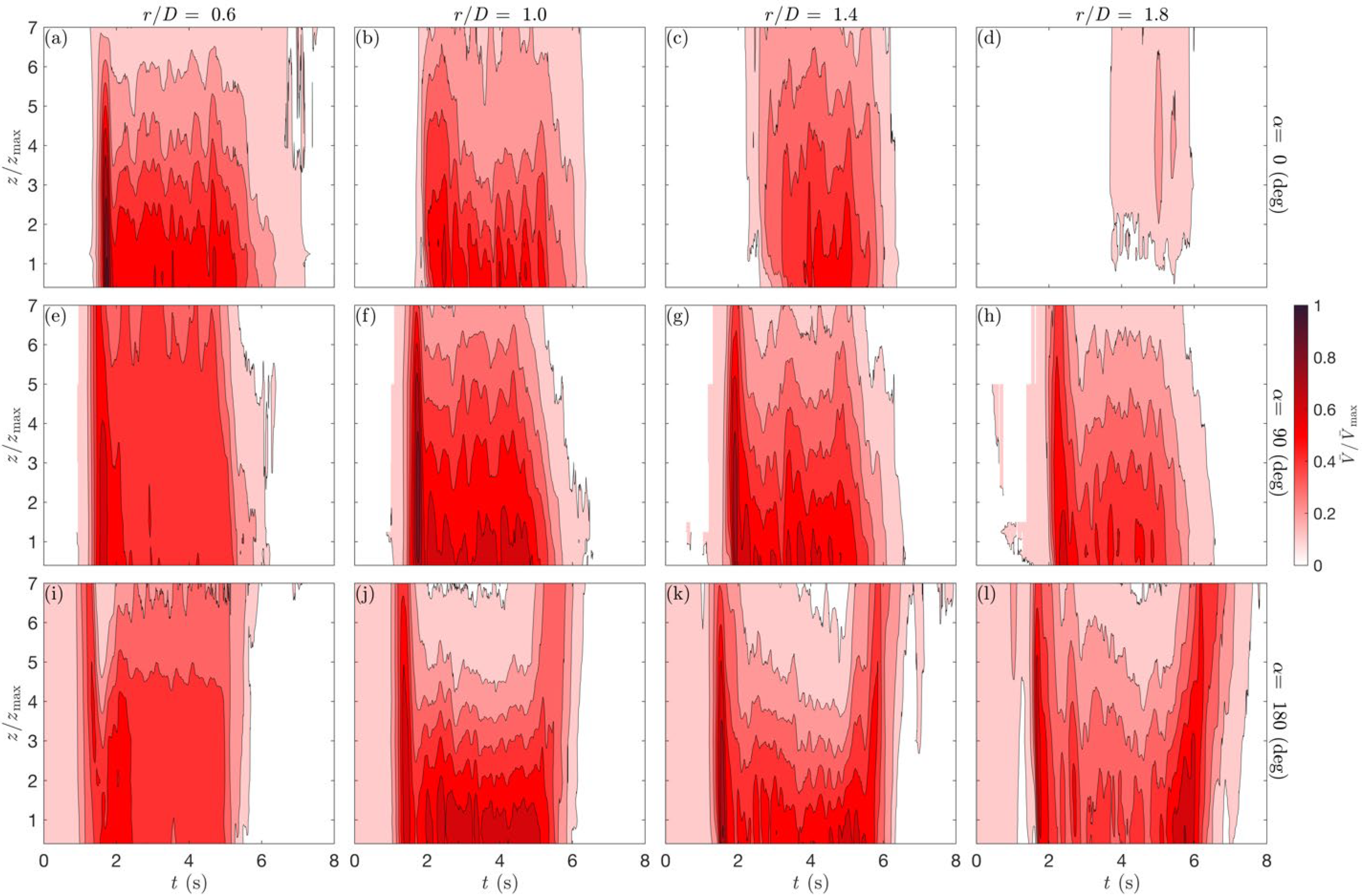
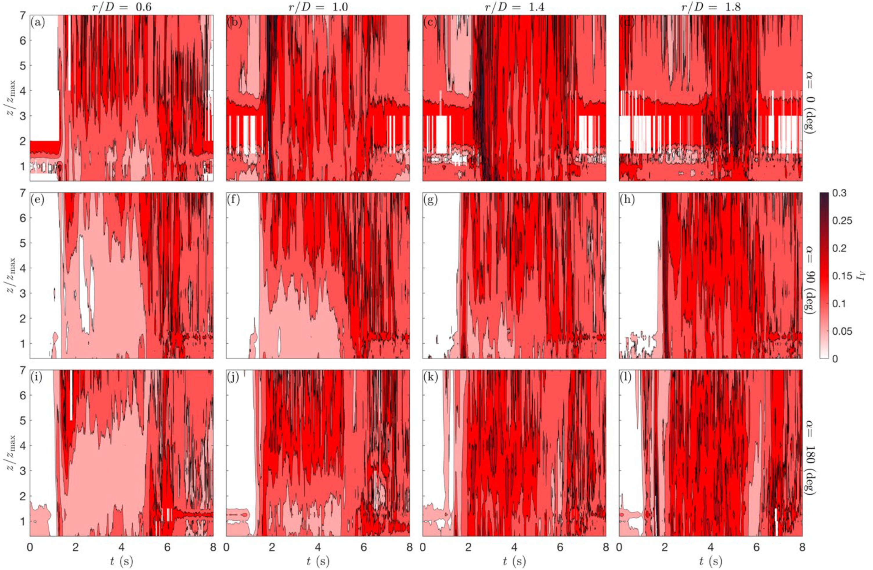
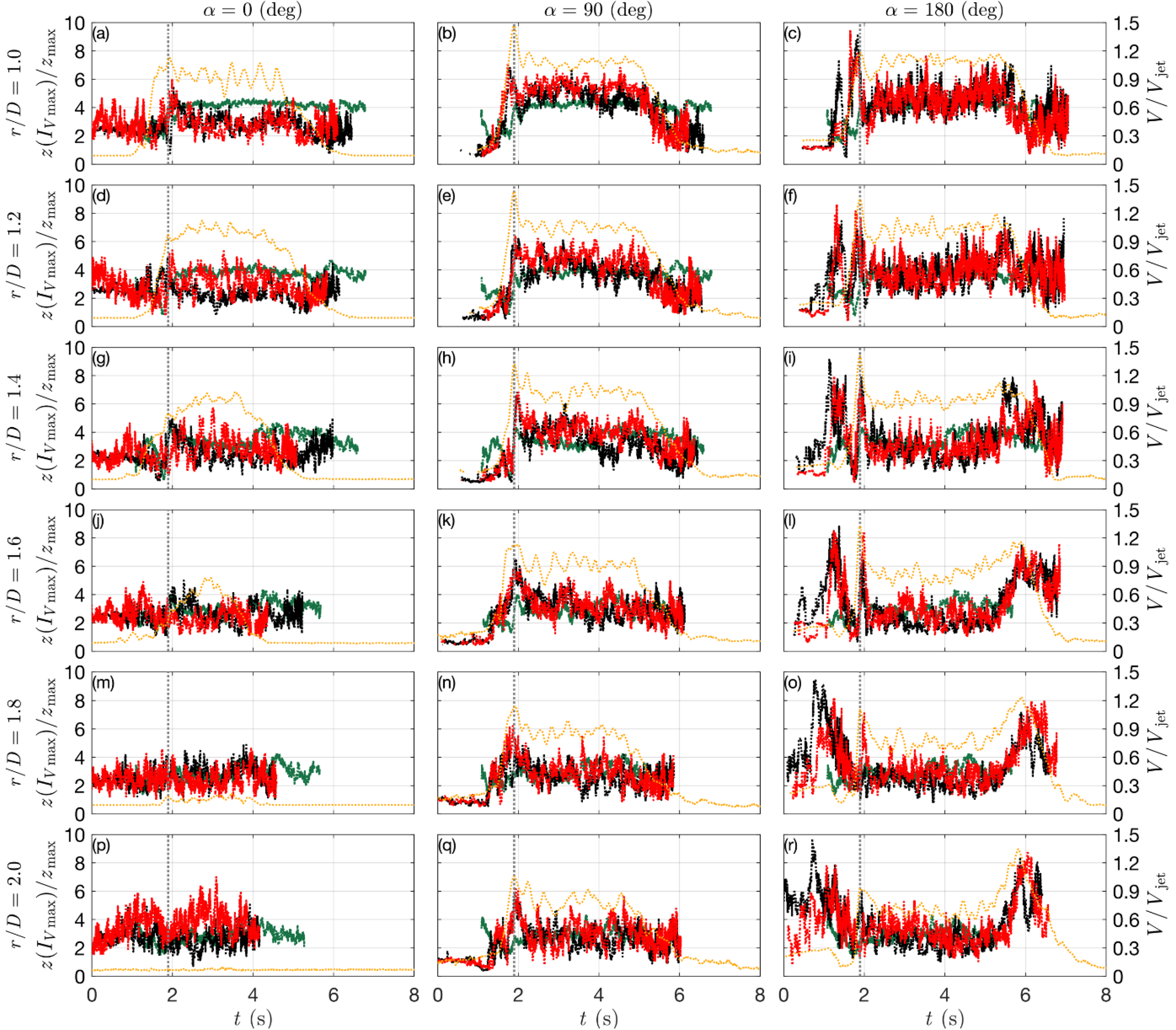
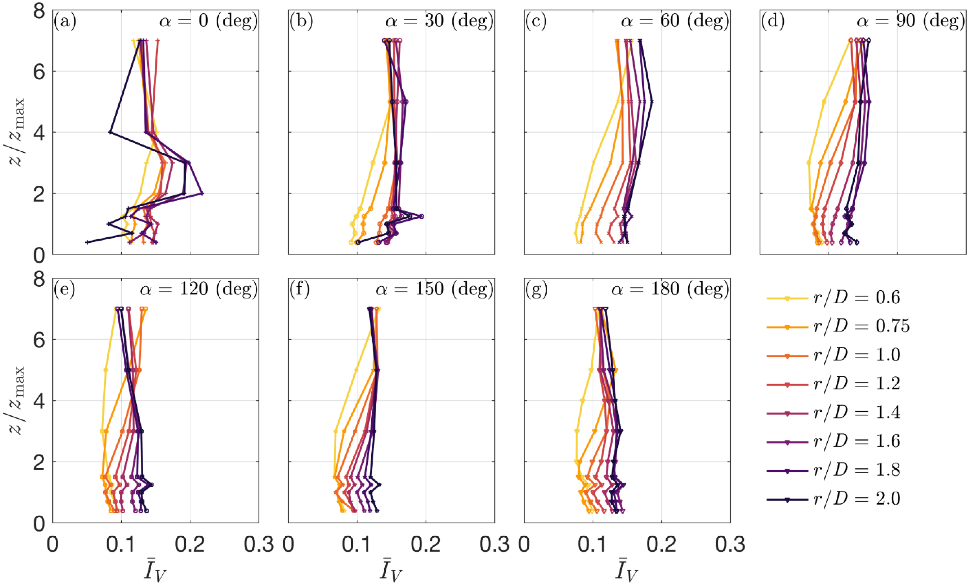
3.6. Turbulence Properties
4. Conclusions and Prospects
Author Contributions
Funding
Acknowledgments
Conflicts of Interest
References
- Solari, G.; Burlando, M.; De Gaetano, P.; Repetto, M.P. Characteristics of Thunderstorms Relevant to the Wind Loading of Structures. Wind Struct. 2015, 20, 763–791. [Google Scholar] [CrossRef]
- Burlando, M.; Zhang, S.; Solari, G. Monitoring, Cataloguing, and Weather Scenarios of Thunderstorm Outflows in the Northern Mediterranean. Nat. Hazards Earth Syst. Sci. 2018, 18, 2309–2330. [Google Scholar] [CrossRef] [Green Version]
- Davenport, A.G. The Application of Statistical Concepts to the Wind Loading of Structures. Proc. Inst. Civ. Eng. 1961, 19, 449–472. [Google Scholar] [CrossRef]
- Davenport, A.G. Gust Loading Factors. J. Struct. Div. 1967, 93, 11–34. [Google Scholar] [CrossRef]
- Goff, R.C. Vertical Structure of Thunderstorm Outflows. Mon. Weather Rev. 1976, 104. [Google Scholar]
- Hjelmfelt, M.R. Structure and Life Cycle of Microburst Outflows Observed in Colorado. J. Appl. Meteorol. 1988, 27, 900–927. [Google Scholar] [CrossRef]
- Canepa, F.; Burlando, M.; Solari, G. Vertical Profile Characteristics of Thunderstorm Outflows. J. Wind Eng. Ind. Aerodyn. 2020, 206, 104332. [Google Scholar] [CrossRef]
- Solari, G.; Burlando, M.; Repetto, M.P. Detection, Simulation, Modelling and Loading of Thunderstorm Outflows to Design Wind-Safer and Cost-Efficient Structures. J. Wind Eng. Ind. Aerodyn. 2020, 200, 104142. [Google Scholar] [CrossRef]
- Solari, G.; Repetto, M.P.; Burlando, M.; De Gaetano, P.; Pizzo, M.; Tizzi, M.; Parodi, M. The Wind Forecast for Safety Management of Port Areas. J. Wind Eng. Ind. Aerodyn. 2012, 104–106, 266–277. [Google Scholar] [CrossRef]
- Repetto, M.P.; Burlando, M.; Solari, G.; De Gaetano, P.; Pizzo, M.; Tizzi, M. A Web-Based GIS Platform for the Safe Management and Risk Assessment of Complex Structural and Infrastructural Systems Exposed to Wind. Adv. Eng. Softw. 2018, 117, 29–45. [Google Scholar] [CrossRef]
- Letchford, C.W.; Chay, M.T. Pressure Distributions on a Cube in a Simulated Thunderstorm Downburst. Part B: Moving Downburst Observations. J. Wind Eng. Ind. Aerodyn. 2002, 90, 733–753. [Google Scholar] [CrossRef]
- Xu, Z.; Hangan, H. Scale, Boundary and Inlet Condition Effects on Impinging Jets. J. Wind Eng. Ind. Aerodyn. 2008, 96, 2383–2402. [Google Scholar] [CrossRef]
- McConville, A.C.; Sterling, M.; Baker, C.J. The Physical Simulation of Thunderstorm Downbursts Using an Impinging Jet. Wind Struct. 2009, 12, 133–149. [Google Scholar] [CrossRef] [Green Version]
- Hangan, H.; Refan, M.; Jubayer, C.; Romanic, D.; Parvu, D.; LoTufo, J.; Costache, A. Novel Techniques in Wind Engineering. J. Wind Eng. Ind. Aerodyn. 2017, 171, 12–33. [Google Scholar] [CrossRef]
- Wood, G.S.; Kwok, K.C.S.; Motteram, N.A.; Fletcher, D.F. Physical and Numerical Modelling of Thunderstorm Downbursts. J. Wind Eng. Ind. Aerodyn. 2001, 89, 535–552. [Google Scholar] [CrossRef]
- Chay, M.T.; Letchford, C.W. Pressure Distributions on a Cube in a Simulated Thunderstorm Downburst—Part A: Stationary Downburst Observations. J. Wind Eng. Ind. Aerodyn. 2002, 90, 711–732. [Google Scholar] [CrossRef]
- Sengupta, A.; Sarkar, P.P. Experimental Measurement and Numerical Simulation of an Impinging Jet with Application to Thunderstorm Microburst Winds. J. Wind Eng. Ind. Aerodyn. 2008, 96, 345–365. [Google Scholar] [CrossRef]
- Mason, M.S.; James, D.L.; Letchford, C.W. Wind Pressure Measurements on a Cube Subjected to Pulsed Impinging Jet Flow. Wind Struct. 2009, 12, 77–88. [Google Scholar] [CrossRef]
- Junayed, C.; Jubayer, C.; Parvu, D.; Romanic, D.; Hangan, H. Flow Field Dynamics of Large-Scale Experimentally Produced Downburst Flows. J. Wind Eng. Ind. Aerodyn. 2019, 188, 61–79. [Google Scholar] [CrossRef]
- Romanic, D.; LoTufo, J.; Hangan, H. Transient Behavior in Impinging Jets in Crossflow with Application to Downburst Flows. J. Wind Eng. Ind. Aerodyn. 2019, 184, 209–227. [Google Scholar] [CrossRef]
- Holmes, J.D.; Hangan, H.M.; Schroeder, J.L.; Letchford, C.W.; Orwig, K.D. A Forensic Study of the Lubbock-Reese Downdraft of 2002. Wind Struct. 2008, 11, 137–152. [Google Scholar] [CrossRef]
- Chay, M.T.; Albermani, F.; Wilson, R. Numerical and Analytical Simulation of Downburst Wind Loads. Eng. Struct. 2006, 28, 240–254. [Google Scholar] [CrossRef] [Green Version]
- Kim, J.; Hangan, H. Numerical Simulations of Impinging Jets with Application to Downbursts. J. Wind Eng. Ind. Aerodyn. 2007, 95, 279–298. [Google Scholar] [CrossRef]
- Abd-Elaal, E.-S.; Mills, J.E.; Ma, X. Empirical Models for Predicting Unsteady-State Downburst Wind Speeds. J. Wind Eng. Ind. Aerodyn. 2014, 129, 49–63. [Google Scholar] [CrossRef]
- Fujita, T.T. Tornadoes and Downbursts in the Context of Generalized Planetary Scales. J. Atmospheric Sci. 1981, 38, 1511–1534. [Google Scholar] [CrossRef] [Green Version]
- Fujita, T.T. The Downburst—Microburst and Macroburst—Report of Projects NIMROD and JAWS; Satellite and Mesometereology Research Project, Dept. of the Geophysical Sciences, University of Chicago, 1985. Available online: http://pi.lib.uchicago.edu/1001/cat/bib/684175 (accessed on 6 January 2020).
- Burlando, M.; Romanić, D.; Solari, G.; Hangan, H.; Zhang, S. Field Data Analysis and Weather Scenario of a Downburst Event in Livorno, Italy, on 1 October 2012. Mon. Weather Rev. 2017, 145, 3507–3527. [Google Scholar] [CrossRef]
- Bray, D.; Knowles, K. Numerical Modeling of an Impinging Jet in Cross-Flow. In Proceedings of the 26th Joint Propulsion Conference, Orlando, FL, USA, 16–18 July 1990. [Google Scholar]
- Barata, J.M.M.; Durào, D.F.G.; Heitor, M.V.; McGuirk, J.J. The Turbulence Characteristics of a Single Impinging Jet through a Crossflow. Exp. Therm. Fluid Sci. 1992, 5, 487–498. [Google Scholar] [CrossRef]
- Barata, J.M.M.; Durão, D.F.G. Laser-Doppler Measurements of Impinging Jet Flows through a Crossflow. Exp. Fluids 2004, 36, 665–674. [Google Scholar] [CrossRef]
- Mason, M.S.; Fletcher, D.F.; Wood, G.S. Numerical Simulation of Idealised Three-Dimensional Downburst Wind Fields. Eng. Struct. 2010, 32, 3558–3570. [Google Scholar] [CrossRef]
- Canepa, F. Physical Investigation of Downburst Winds and Applicability to Full Scale Events. Doctoral Thesis, University of Genoa, Genoa, Italy, Western University, London, ON, Canada, 2022. [Google Scholar]
- Richter, A.; Ruck, B.; Mohr, S.; Kunz, M. Interaction of Severe Convective Gusts with a Street Canyon. Urban Clim. 2018, 23, 71–90. [Google Scholar] [CrossRef]
- Romanic, D.; Hangan, H. The Interplay Between Background Atmospheric Boundary Layer Winds and Downburst Outflows. A First Physical Experiment. In Proceedings of the XV Conference of the Italian Association for Wind Engineering; Ricciardelli, F., Avossa, A.M., Eds.; Springer International Publishing: Cham, Switzerland, 2019; Volume 27, pp. 652–664. ISBN 978-3-030-12814-2. [Google Scholar]
- Romanic, D.; Hangan, H. Experimental Investigation of the Interaction between Near-Surface Atmospheric Boundary Layer Winds and Downburst Outflows. J. Wind Eng. Ind. Aerodyn. 2020, 205, 104323. [Google Scholar] [CrossRef]
- Romanic, D.; Nicolini, E.; Hangan, H.; Burlando, M.; Solari, G. A Novel Approach to Scaling Experimentally Produced Downburst-like Impinging Jet Outflows. J. Wind Eng. Ind. Aerodyn. 2020, 196, 104025. [Google Scholar] [CrossRef]
- Behnia, M.; Parneix, S.; Shabany, Y.; Durbin, P.A. Numerical Study of Turbulent Heat Transfer in Confined and Unconfined Impinging Jets. Int. J. Heat Fluid Flow 1999, 20, 1–9. [Google Scholar] [CrossRef]
- Romanic, D.; Chowdhury, J.; Chowdhury, J.; Hangan, H. Investigation of the Transient Nature of Thunderstorm Winds from Europe, the United States, and Australia Using a New Method for Detection of Changepoints in Wind Speed Records. Mon. Weather Rev. 2020, 148, 3747–3771. [Google Scholar] [CrossRef]
- Wakimoto, R.M. The Life Cycle of Thunderstorm Gust Fronts as Viewed with Doppler Radar and Rawinsonde Data. Mon. Weather Rev. 1982, 110, 1060–1082. [Google Scholar] [CrossRef] [Green Version]
- Canepa, F.; Burlando, M.; Romanic, D.; Solari, G.; Hangan, H. Downburst-like Experimental Measurements of Two Vertical-Axis Impinging Jets at the WindEEE Dome. PANGAEA 2021. [Google Scholar] [CrossRef]
- Lombardo, F.T.; Smith, D.A.; Schroeder, J.L.; Mehta, K.C. Thunderstorm Characteristics of Importance to Wind Engineering. J. Wind Eng. Ind. Aerodyn. 2014, 125, 121–132. [Google Scholar] [CrossRef]
- Alahyari, A.; Longmire, E.K. Dynamics of Experimentally Simulated Microbursts. AIAA J. 1995, 33, 2128–2136. [Google Scholar] [CrossRef]
- Zhang, S.; Solari, G.; De Gaetano, P.; Burlando, M.; Repetto, M.P. A Refined Analysis of Thunderstorm Outflow Characteristics Relevant to the Wind Loading of Structures. Probabilistic Eng. Mech. 2018, 54, 9–24. [Google Scholar] [CrossRef]
- Zhang, S.; Solari, G.; Burlando, M.; Yang, Q. Directional Decomposition and Properties of Thunderstorm Outflows. J. Wind Eng. Ind. Aerodyn. 2019, 189, 71–90. [Google Scholar] [CrossRef]
- Gauntner, J.W.; Livingood, J.N.B.; Hrycak, P. Survey of Literature on Flow Characteristics of a Single Turbulent Jet Impinging on a Flat Plate; NASA Lewis Research Center: Cleveland, OH, USA, 1970; p. 46. [Google Scholar]
- Gogineni, S.; Shih, C. Experimental Investigation of the Unsteady Structure of a Transitional Plane Wall Jet. Exp. Fluids 1997, 23, 121–129. [Google Scholar] [CrossRef]
- Alcântara Pereira, L.A.; de Oliveira, M.A.; de Moraes, P.G.; Bimbato, A.M. Numerical Experiments of the Flow around a Bluff Body with and without Roughness Model near a Moving Wall. J. Braz. Soc. Mech. Sci. Eng. 2020, 42, 129. [Google Scholar] [CrossRef]
- Mimeau, C.; Mortazavi, I. A Review of Vortex Methods and Their Applications: From Creation to Recent Advances. Fluids 2021, 6, 68. [Google Scholar] [CrossRef]


| Case | D [m] | Vjet [m s−1] | VABL [m s−1] | α [°] | r/D [/] | z/zmax [m] | Reps |
|---|---|---|---|---|---|---|---|
| DBABL5.0 | 3.2 | 12.4 | 2.5 | 0:30:180 | 0.2:0.2:2 | : 0.4, 0.7, 1.0, 1.25, 1.5, 3.0, 5.0, 7.0 (IJ) 0.4, 1.0, 3.0, 5.0 (SF) : 0.4, 0.7, 1.0, 1.25, 1.5, 2.0, 3.0, 4.0, 7.0 (IJ) : 0.4, 0.7, 1.0, 1.25, 1.5, 2.0, 3.0, 4.0, 5.0, 7.0, 10.0 (IJ) | 10 |
| DBABL3.0 | 3.2 | 11.8 | 3.9 | 0:30:180 | 0.2:0.2:2 | “ | 10 |
| Case | |
|---|---|
| DBABL5.0 (DB-like flow) | 2.7 106 |
| DBABL5.0 (ABL-like flow) | 6.4 105 |
| DBABL3.0 (DB-like flow) | 2.6 106 |
| DBABL3.0 (ABL-like flow) | 1.0 106 |
| DBABL3.0 (DBABL-like flow) | 1.4 105 |
| DBABL3.0 (DBABL-like flow) | 1.4 105 |
| Acquisition frequency | 2500 Hz |
| Cut-off frequency factor | 0.5 |
| Cut-off frequency | 250 Hz |
| Accuracy of velocity measurements | ± 0.5 m s−1 * |
| Accuracy of yaw and pitch angles | ± 1° * |
| Measurement cone of incoming flow | ± 45° ** |
Publisher’s Note: MDPI stays neutral with regard to jurisdictional claims in published maps and institutional affiliations. |
© 2022 by the authors. Licensee MDPI, Basel, Switzerland. This article is an open access article distributed under the terms and conditions of the Creative Commons Attribution (CC BY) license (https://creativecommons.org/licenses/by/4.0/).
Share and Cite
Canepa, F.; Burlando, M.; Hangan, H.; Romanic, D. Experimental Investigation of the Near-Surface Flow Dynamics in Downburst-like Impinging Jets Immersed in ABL-like Winds. Atmosphere 2022, 13, 621. https://0-doi-org.brum.beds.ac.uk/10.3390/atmos13040621
Canepa F, Burlando M, Hangan H, Romanic D. Experimental Investigation of the Near-Surface Flow Dynamics in Downburst-like Impinging Jets Immersed in ABL-like Winds. Atmosphere. 2022; 13(4):621. https://0-doi-org.brum.beds.ac.uk/10.3390/atmos13040621
Chicago/Turabian StyleCanepa, Federico, Massimiliano Burlando, Horia Hangan, and Djordje Romanic. 2022. "Experimental Investigation of the Near-Surface Flow Dynamics in Downburst-like Impinging Jets Immersed in ABL-like Winds" Atmosphere 13, no. 4: 621. https://0-doi-org.brum.beds.ac.uk/10.3390/atmos13040621