Article

Assessment of Quarterly, Semiannual and Annual Models to Forecast Monthly Rainfall Anomalies: The Case of a Tropical Andean Basin

by
Angel Vázquez-Patiño
1,2,3,
Mario Peña
4 and
Alex Avilés
5,6,*
1
Departamento de Ingeniería Civil, Universidad de Cuenca, Cuenca 010207, Ecuador
2
Facultad de Ingeniería, Universidad de Cuenca, Cuenca 010207, Ecuador
3
Facultad de Arquitectura, Universidad de Cuenca, Cuenca 010203, Ecuador
4
Departamento de Química Aplicada y Sistemas de Producción, Facultad de Ciencias Químicas, Universidad de Cuenca, Cuenca 010203, Ecuador
5
Grupo de Evaluación de Riesgos Ambientales en Sistemas de Producción y Servicios (RISKEN), Eco Campus Balzay, Universidad de Cuenca, Cuenca 0101168, Ecuador
6
Carrera de Ingeniería Ambiental, Facultad de Ciencias Químicas, Eco Campus Balzay, Universidad de Cuenca, Cuenca 0101168, Ecuador
*
Author to whom correspondence should be addressed.
Submission received: 26 April 2022 / Revised: 25 May 2022 / Accepted: 26 May 2022 / Published: 31 May 2022

Abstract

:
Rainfall forecasting is essential to manage water resources and make timely decisions to mitigate adverse effects related to unexpected events. Considering that rainfall drivers can change throughout the year, one approach to implementing forecasting models is to generate a model for each period in which the mechanisms are nearly constant, e.g., each season. The chosen predictors can be more robust, and the resulting models perform better. However, it has not been assessed whether the approach mentioned above offers better performance in forecasting models from a practical perspective in the tropical Andean region. This study evaluated quarterly, semiannual and annual models for forecasting monthly rainfall anomalies in an Andean basin to show if models implemented for fewer months outperform accuracy; all the models forecast rainfall on a monthly scale. Lagged rainfall and climate indices were used as predictors. Support vector regression (SVR) was used to select the most relevant predictors and train the models. The results showed a better performance of the annual models mainly due to the greater amount of data that SVR can take advantage of in training. If the training of the annual models had less data, the quarterly models would be the best. In conclusion, the annual models show greater accuracy in the rainfall forecast.

1. Introduction

Rain is a phenomenon that significantly conditions human activity. Knowing its dynamics and forecasting its behavior is essential to optimize water use, for example, in human consumption, hydroelectric generation, agriculture [1], and industry. On the other hand, anticipating extreme rainfall events helps to take measures to mitigate possible adverse effects (e.g., landslides, floods, and droughts). Examples of such extreme events are the droughts in the Southwest US [2], the São Francisco river basin (Brazil) [3], the northeast region of Brazil [4,5], and over Brazil [6]. Additionally, rain is an essential atmospheric variable to characterize the climate [7]. Therefore, unveiling the drivers related to this hydrologic process is essential to understanding possible changes in its dynamics under low-frequency natural climate variability [8] or climatic change [9].
Different models allow us to anticipate rain behavior. There are different methods that can be used to make predictions. Dynamic models are physically consistent [10], but these have a tremendous computational burden. Instead, statistical methods are widely used to identify the main modes of climate variability at different spatial and temporal scales [11]. In addition, some models use a combination of the two approaches [12]. Weather and seasonal forecasting models or decadal prediction models could be developed depending on the forecast horizon. From an operational point of view, and in terms of relevance for short- and medium-term decision-makers, intraseasonal and seasonal forecasting models are the most important. They consider forecasts from two months to a little over a year [13,14] and help in tasks such as those listed above. Moreover, different data-based approaches are used when constructing forecasting models such as those based on autoregressive models (e.g., [15]), empirical models (e.g., [14]) or others that are more robust, such as those based on machine learning (ML) techniques (e.g., [16,17]) or network science (e.g., [18,19]). Likewise, models can be constructed based on different candidate predictors such as exogenous variables (e.g., [17,20]) or climate indices (e.g., [21,22]).
Seasonality is a remarkable feature in nature, and different precursors defining rainfall also have temporal variability [23] (change in mechanisms [24]). Moreover, heterogeneous rainfall magnitudes through the year could negatively affect the performance of a single model in forecasting the rainfall of each month of a year. Depending on the algorithm/model used to train the forecasting model, scaling and/or standardization are frequently used preprocessing methods [25]. The rainfall anomalies are commonly computed, which helps eliminate seasonality and allows unexpected values beyond trivial behavior (mainly affected by seasonal solar irradiance) to be forecasted. However, the changing influence of predictors over the target variable (rainfall) is an implicit feature that is still present. So, an alternative is to construct models for each semester, season or even month of the year [24] (e.g., [26]). Following the premise of changing mechanisms throughout the year, such an alternative aims to learn the relationships between predictors and rainfall in different seasons or periods of wet or dry behavior to have better-performing models. This is because the predictors may provide information that makes the models more robust. However, as far as the authors know, an assessment to determine if subannual models perform better has not been carried out, and less is known about mountain zones such as the Andes where complex processes dominate the rainfall behavior throughout the year [27,28,29].
This study aimed to determine if the performance of anomaly rainfall forecasting models improved as the models were developed for each quarter, each semester or the whole year with a horizon of one year. These models always aim to forecast monthly rainfall and differ in the months for which they can make the forecast. For example, one of the quarterly models allows one to forecast the rainfall of December, January, and February (there are four quarterly models in total), one of the semiannual models forecasts the rainfall from November to April (there are two semiannual models), and the annual model forecasts the rainfall of any month of the year. In addition, the influence of predictors based on large-scale climatic factors on these improvements was analyzed. For this, three sets of anomaly rainfall forecasting models were trained through the support vector regression algorithm. The first set constituted the four quarterly models to forecast rainfall each season. The second set contained the two semiannual models, and the third referred to the annual model. Each model used an independent subset of lagged climate indices and anomaly rainfall signals as predictors. Such subsets were chosen by employing the sequential feature selection algorithm. Finally, the models were assessed by utilizing seven evaluation metrics.

2. Materials and Methods
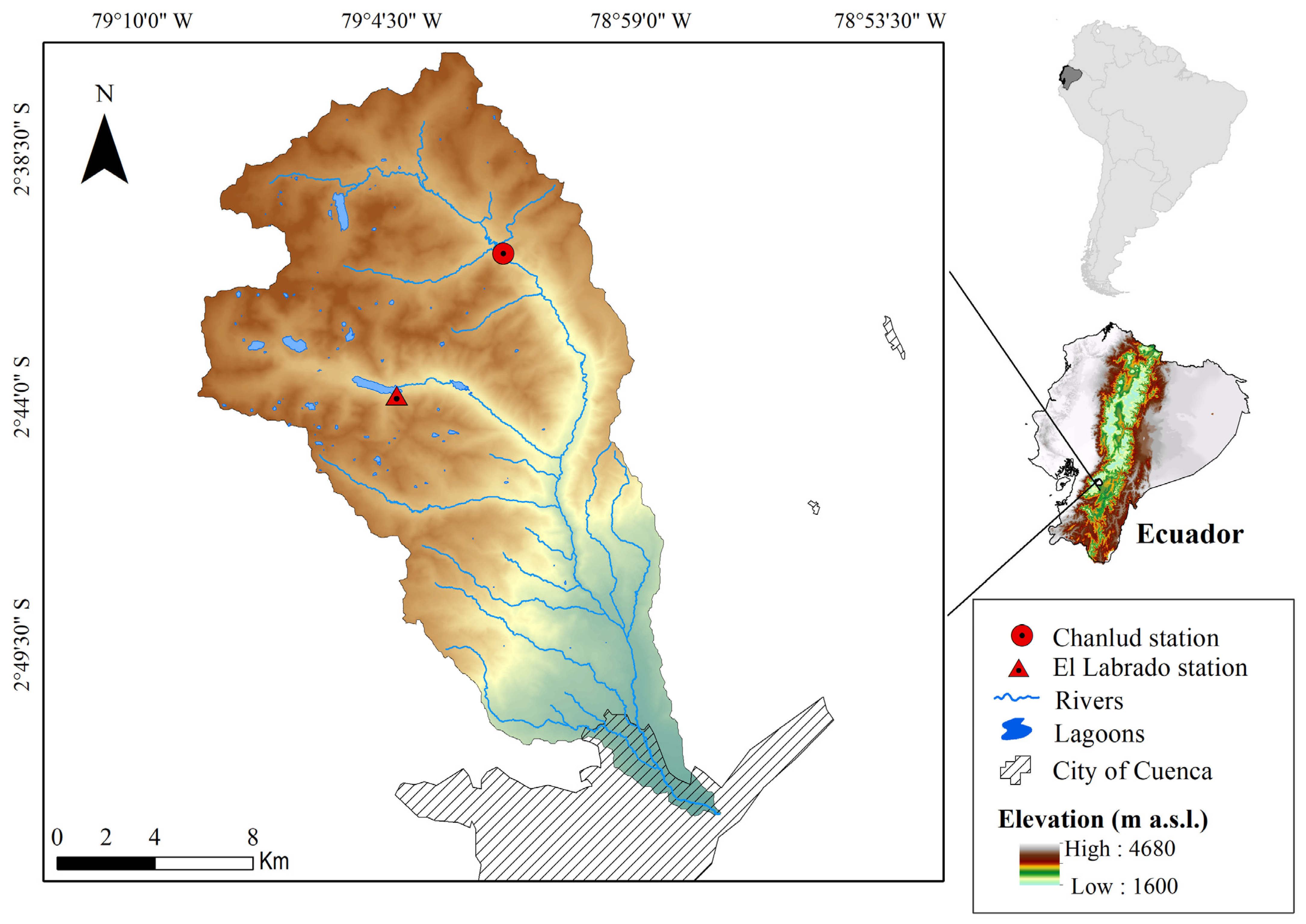
2.1. Study Zone

The Machángara river basin is located northeast of Cuenca, the capital city of Azuay, in the Andes mountain range of southern Ecuador (Figure 1). The basin area is approximately 325 km2 and has a high altitudinal gradient extending from 2440 to 4420 m a.s.l. Natural areas form the upper part of this basin, agricultural activities mainly occupy the middle part, with small-urbanized patches, and urbanized sectors characterize the lower part [30]. The rainfall varies from 856 to 1309 mm, while the temperature ranges from 8.1 to 14 °C [31]. The Pacific Ocean, the Andes range and the Amazon basin mainly influence the climate of this region [29,32,33].
The integrated management of natural resources in the Machángara basin guarantees the provision of essential services, for example, water for human consumption for more than 390,000 inhabitants of Cuenca (≅60% of the population), irrigation for more than 3900 users, the generation of 39.5 MW of hydroelectricity (the first source of electric energy in Ecuador [34]), and the provision of water for various industries in the area. In the highest part of the basin, two representative stations were selected for the study, namely El Labrado and Chanlúd, which are at approximately 3335 and 3485 m a.s.l., respectively. The two stations are located in the dams that bear the same names [35] and are greatly important in the national hydroelectric generation system.

2.2. Data

The daily rainfall data of El Labrado and Chanlúd go back to 1964 and 1981, respectively. This study used monthly rainfall data from 1981 to 2021 (41 y). Therefore, the daily rainfall corresponding to each month of the period 1981–2021 was added to generate data on a monthly scale. Figure 2a shows the monthly rainfall data of El Labrado and Chanlúd in the study period. Rainfall shows a marked bimodal seasonality, which is shown in Figure 2b. A peak of heavy rain is present in April, while the driest month is August.
The target variable of the forecasting models is the rainfall anomalies. Most of the predictors of such models are based on climate indices. Table 1 shows the 38 climate indices used in the study, which have a monthly resolution. Thirty-four were downloaded from the National Oceanic and Atmospheric Administration (NOAA) (https://psl.noaa.gov/data/climateindices/list/, accessed on 21 January 2022), and the sources of the rest are indicated in the table footer.
Both rainfall and climate indices constitute the raw monthly dataset. The dataset was split into training and testing subsets. The former spanned from 1981 to 2015 (35 y) and the latter from 2016 to 2021 (6 y). Figure 2a shows the training subset period in a white background, while the testing period is shaded. The training subset was used to compute rainfall anomalies, standardize the dataset, generate and select predictors, and train the forecasting models. The testing subset was only used to evaluate the performance of the models. It is worth noting that the standardization of the testing subset was based on the parameters found in the training subset. The latter ensures an adequate evaluation since it simulates a scenario in which nothing is known beyond the data available for model training.

2.3. Settings and Workflow

This subsection explains the workflow followed in the study in a general manner. The following subsections describe details about data or methods in each step. So, Scheme 1 shows the workflow to assess the quarterly, semiannual and annual models to forecast monthly rainfall anomalies.
The first step shown in Scheme 1 is the deseasonalization of rainfall. The monthly rainfall climatology (Figure 2b) was computed based on the training subset period (1981–2015). Then, the climatology was subtracted from the raw rainfall signal. The second step is the standardization of the rainfall anomalies and climate indices data by removing the mean and scaling to unit variance. The Standard Scaler from the Scikit-learn library [52] was used in this step. As an example, Figure 2c shows the scaled and standardized rainfall anomalies. The shaded period in Figure 2c was not used to compute the parameters in the scaling and standardization. The third step is the generation of the candidate predictor set. For this, lagged versions of the time series of the rainfall anomalies and climate indices were generated up to a maximum τ lag (τmax) which was chosen through an autocorrelation analysis. These signal delays are operationally essential to generate predictors with past information that serve the current forecast, anticipating the decision making.
The fourth step is the selection of relevant predictors for each forecasting model. For each forecasting model, different subsets of relevant predictors were selected (dashed squares in step 4) through the sequential forward selection (SFS) algorithm. There were seven different subsets for four quarterly models, two semiannual models, and one annual model. The quarterly models forecast anomaly rainfall of months belonging to each of the four seasons (e.g., the DJF model predicts rainfall in Dec–Feb), the semiannual models forecast rainfall of months belonging to each of the two semesters (e.g., the NDJFMA model forecasts rainfall in November–April), and the annual model forecasts rainfall of any month of the year. In any case, the forecasting horizon was one year. Those seven models were trained in the fifth step shown in Scheme 1. The forecasting models were based on the support vector regression (SVR) learning algorithm [53].
The last step is the evaluation. Each year of rainfall was forecasted independently for the testing subset period (2016–2021). With the entire testing period, a qualitative comparison was first made. Then, the evaluation was performed with seven evaluation metrics (the models had a horizon of one year). The comparison was performed with the raw testing rainfall data, so the results of the models were firstly converted (seasonalization) to the original scale (based on the parameters of the training subset).

2.4. Maximum τ lag (τmax)

In order to choose the τmax for the generation of candidate predictors, the autocorrelation of the raw rainfall signals was used. Each station’s autocorrelation function (ACF) was plotted with 95% confidence intervals employing the statsmodels library [54]. These confidence intervals suggest that the correlation values within them are likely a statistical fluke. The standard deviation computation for the confidence intervals was performed according to Bartlett’s formula [55,56].
The 38 climate indices from which the candidate predictors were derived had a particular τmax, after which, the correlation with rainfall (target variable) was no longer significant. Beyond an analysis of autocorrelations, an exhaustive analysis of lagged cross-correlations (such as in [57]) would allow one to obtain a τmax for each index concerning the target variable and to possibly achieve higher-performance forecasting models. In addition, the above should have been taken into account for both El Labrado and Chanlúd rainfall. This would have led to 39 different τmax for each station. However, in order not to divert the study from the objective pursued, only the autocorrelation of rainfall was taken into account. Once the autocorrelation graphs of each station were analyzed, a single reasonable τmax value was taken through the study.

2.5. Generation of Candidate Predictor Sets

Four quarterly models were trained, one by each season, i.e., DJF, MAM, JJA and SON, two semiannual models related to semesters November–April (NDJFMA) and May–October (MJJASO) and one annual model (J-D). These models were schematized as blank squares in step five in Scheme 1. The forecasting horizon was one year, and as an example, if one wanted to forecast rainfall for 2016, January rainfall would be forecasted with the DJF model. Such a value would be immediately used as a possible predictor to forecast the February rainfall with the DJF model. The MAM model would be used to forecast March rainfall, and the same for April and May rainfall. The exact process would be used to forecast the rest of the months. Thus, the following lags were used for each forecasting model to generate the candidate predictor sets.
Candidate predictor set for quarterly models:
  • DJF: 13 to τmax.
  • MAM: 6 to τmax.
  • JJA: 9 to τmax.
  • SON: 12 to τmax.
Candidate predictor set for semiannual models:
  • NDJFMA: 13 to τmax.
  • MJJASO: 11 to τmax.
Candidate predictor set for annual models:
  • J-D: 13 to τmax.
The minimum limit of each interval shown above allows one to leverage as much information as possible. For instance, for forecasting March–May rainfall using the MAM model, information with a minimum lag of six means that information from November of the previous year could be used.

2.6. Sequential Forward Selection (SFS) of Predictors

The sequential forward selection (SFS) is a greedy approach to selecting the best new predictor iteratively from the candidate predictor set to aggregate to a subset of selected predictors [58]. The algorithm initially finds one predictor (the first) that maximizes a cross-validated score when a learning algorithm is trained on this single predictor. After the first (best) predictor is selected, the algorithm finds the second predictor that maximizes the score of the learning algorithm when it is trained on these two single predictors. The process is repeated by adding new predictors to the subset of selected predictors in each iteration. The optimum subset of relevant predictors is the one that gives the best cross-validated performance. There are different implementations of the SFS algorithm, and here, the one from the MLxtend library [59] was used. Moreover, this study used the support vector regression (SVR) learning algorithm to compute the score based on the selected predictor subsets. The SVR implementation of the Scikit-learn library [52] was used with the default hyperparameters. The cross-validated score was obtained through 5-fold cross-validation.

2.7. Support Vector Regression (SVR)

The support vector regression (SVR) model was proposed by Vapnik [60] and is a suitable model for linear and nonlinear regression. SVR is based on elements of the support vector machine (SVM), where support vectors are the closest points toward the generated hyperplane in a high-dimensional feature space [53]. As in most machine learning models, the training data are divided into two subsets: the training and validation sets [61]. The SVR model maps the training data to a high-dimensional feature space using a kernel. The radial basis function (RBF) kernel was used in this study. The hyperparameters are then optimized (i.e., model training) by fitting the model to the training data in that feature space. The formal definition of the SVR model is as follows.
Given { x i , y i } denoted as a characteristic vector of sample data with i = 1 ,   2 ,   ,   m samples, where x i ϵ n , n is the number of predictors, and y i ϵ is the target variable (rainfall anomalies). The SVM regression estimation function is defined as
f ( x ) = W T ϕ ( x ) + b
where W T is the weights matrix of the independent function, ϕ ( x ) is the nonlinear (kernel) mapping function, and b is the intercept. Then, W T and b can be obtained by minimizing the equation
M i n : 1 2 | | W | | 2 + C m i = 1 m R ε [ y i , f ( x i ) ]
where | | W | | 2 is known as regularized term; C is the penalty parameter; and R ε is the insensitive loss function (error control function) of the margin of tolerance ε .
The SVR model generally requires a small sample size for training, has a simple statistical structure and performs better than complex models, e.g., artificial neural networks.
In the model training, the training data were not only divided into a new training subset and a validation subset. Instead, the 5-fold cross-validation technique was used to gain generalization. A particular subset of predictors for each forecasting model was used (dashed squares of step 4 in Scheme 1). Moreover, the following set of values for each of the hyperparameters was used in the training process:
  • C = { 2 i i , 20 i 10 } ;
  • ε = { 2 i i , 20 i 10 } ;
  • γ = { 2 20 + 19 30 i i , 0 i 30 } .
The γ hyperparameter corresponds to the RBF kernel used and relates to the inverse of the radius of influence of registers selected by the model as support vectors. The number of models trained until the best-performing one is found for each forecasting model is 31,713 × 5 = 158,565 (31,713 hyperparameter combinations, and 5 corresponds to the 5-fold cross-validation).

2.8. Evaluation Metrics

Given the raw rainfall time series y = { y 1 , y 2 , , y m } and the seasonalized forecasted rainfall y ^ = { y ^ 1 , y ^ 2 , , y ^ m } , the forecasting models were evaluated with the following seven metrics. These metrics are commonly used for evaluating forecasting and prediction models [62,63,64,65].
Mean Absolute Relative Error (MARE). The MARE measures how much error exists in the forecasted rainfall relative to the observed values in absolute terms. It is computed by
MARE = i = 1 m | y i y ^ i | i = 1 m y i
The MARE is independent of the time series scale, and its value ranges from 0 to ∞, with 0 being the measure of a perfect forecast.
Mean Absolute Error (MAE). The MAE represents the average of the absolute difference between the forecasted values and the observations. It measures the average of the residuals regardless of their sign. The MAE is defined as
MAE = 1 m i = 1 m | y i y ^ i |
This metric scale depends on the scale of rainfall, and its value ranges from 0 to ∞, with 0 being the best value.
Root Mean Square Error (RMSE). The RMSE is the square root of the average of the squared difference between the forecasted values and the observations. The RMSE is defined as
RMSE = 1 m i = 1 m ( y i y ^ i ) 2
The RMSE values are dependent on the time-series scale, and its value ranges from 0 to ∞, with 0 being the measure for a perfect forecast.
Nash–Sutcliffe Efficiency (NSE). The NSE [66] is widely used to evaluate the performance of hydrological models. Although the NSE is susceptible to outliers because it takes a sum over the squared values of the differences between the forecasted values and the observations, it is even better than other metrics, such as the coefficient of determination. The NSE is defined as
NSE = 1 i = 1 m ( y i y ^ i ) 2 i = 1 m ( y i y - ) 2
where y - is the average of the rainfall time series (observations). The scale of this metric is independent of the scale of the rainfall values. The values of this metric go from −∞ to 1, with 1 meaning perfect forecasting, 0 meaning that the results are as good as always using y - for the forecasting and negative values meaning arbitrarily bad results.
Kling–Gupta Efficiency (KGE). The KGE [67] is a robust performance measure based on three equally weighted components: variability, linear correlation, and bias ratio between forecasted and observed rainfall. The KGE is defined as
K G E = 1 ( α 1 ) 2 + ( c c 1 ) 2 + ( β 1 ) 2
where α is the variability (the ratio between the standard deviation of forecasted rainfall over the observed rainfall), c c is the linear correlation coefficient between forecasted and observed values, and β is the division between the average of the forecasted rainfall over the average of the observed rainfall.
The KGE is independent of the rainfall scale, and its value goes from −∞ to 1. The higher the value, the better the forecast.
Explained Variance (EV). The EV measures the proportion of the variance of the residuals (differences between y i and y ^ i ) and the rainfall variance. It is computed by
EV = 1 i = 1 m [ ( y i y ^ i ) 1 m j = 1 m ( y j y ^ j ) ] 2 i = 1 m ( y i y - ) 2
The EV is independent of the time series scale, and its value ranges from −∞ to 1, with 1 being the optimum value and negative values indicating arbitrarily bad forecasting results. EV = 0 indicates that the model is as good as using any fixed value for the forecast.
Percent Bias (PBIAS). The PBIAS determines whether there is a tendency in the values forecasted by the model (i.e., if these are higher or lower than the observed values). A positive PBIAS indicates that the model overestimates the forecasted variable, while a negative value indicates that the variable is underestimated. The optimal value is a PBIAS equal to zero. This metric is defined as
PBIAS = 100 × i = 1 m ( y ^ i y i ) i = 1 m y i
This metric is independent of the rainfall scale, and the closer the value of |PBIAS| to 0, the better the results, with 0 being the optimum value. |PBIAS| values greater than 100 indicate arbitrarily bad results.

3. Results

3.1. τmax for Generating the Candidate Predictors

Figure 3 shows the ACFs of El Labrado and Chanlúd rainfall. The autocorrelation demonstrated a high seasonal rainfall signal with statistical significance until 37 months in El Labrado and 49 months in Chanlúd. A lag of 37 months was then taken as the τmax to create the candidate predictor set. Since this study concentrates on comparing models differing in the number of months used in the implementation, the same number of 37 lags was taken as the maximum to create the candidate predictors based on the 38 climate indices (Table 1).

3.2. Optimum Number of Predictors

Figure 4 shows the results of selecting the optimum number of predictors through the SFS approach. Each column corresponds to the different model sets, i.e., quarterly, semiannual and annual models. Each row corresponds to the models for El Labrado and Chanlúd. The performance behavior of the models showed a similar tendency. The optimum number of predictors was around 81 and 68 for El Labrado and Chanlúd, respectively. The optimum number of predictors for quarterly, semiannual and annual models for El Labrado were around 93, 73 and 55, respectively. Meanwhile, for Chanlúd, the optimum numbers were around 69, 49 and 105. However, the performance of the annual model for Chanlúd (Figure 4f) had a lower variance in the approximated interval of 35–105 predictors. Thus, the greater the number of months that are considered in the models with different periods, the fewer the predictors that are needed to get the best performance. A possible explanation for this behavior is the greater number of records (instances) that the models had in the training stage of the SFS as they were built for more months (e.g., annual models). The annual models used 100% of the available records in the selection of predictors (383 of the 420 because of the candidate predictor generation with 37 lags), the semiannual models used 50% of such records (November–April: 191, May–October: 192), and the quarterly models used 25% (DJF: 95, MAM: 96, JJA: 96, SON: 96). The SFS used the SVR learning algorithm with the default hyperparameters, so varying the number of records changed the amount of relevant information for the forecasting. From a purely predictive point of view, models for more months achieve better performance with fewer predictors that have more relevant information to achieve better generalization.

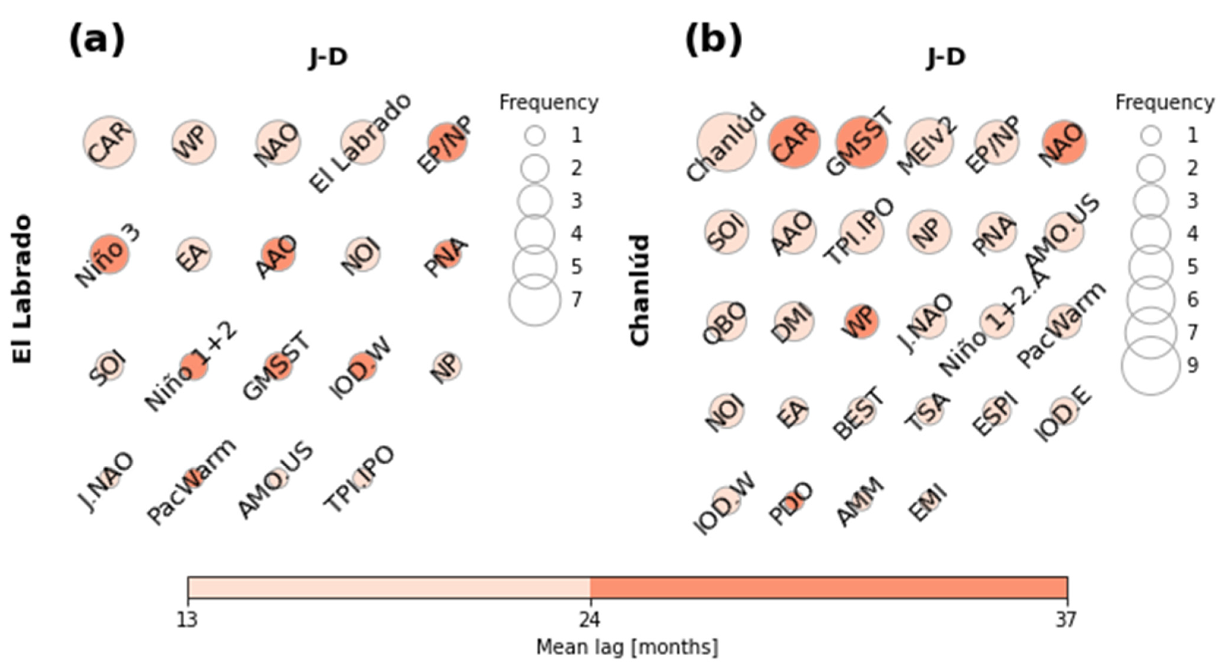
3.3. Relevant Predictors

The optimum number of predictors allows light to be shed on the more prominent indices to predict rainfall anomalies in the stations of the study zone. First, quarterly models allowed indices influencing each season to be analyzed. The analysis was conducted using the times an index with different lags was chosen. This number is labeled the frequency in Figure 5, Figure 6, Figure 7 and Figure 8. The mean number of lags of the different indices chosen are shown in intervals of up to 12 months, 24 months and more than 24 months.
Figure 5 shows the climate indices providing more information for the predictor selection stage in each season for El Labrado. The most prominent feature was the EP/NP climate index in all seasons. In all the seasons, the EP/NP mean lag was within the 12 months before the rainfall value that had to be forecasted. The NP index was the second most prominent feature present in the models for the four seasons. NP was the second most prominent in DJF and SON, third in MAM, and sixth in JJA. Like EP/NP, the NP mean lag was within 12 months before the forecasted rainfall value. The Niño 3 index was present within the seven most prominent indices in DJF and MAM. DJF is a season when the climate conditions of the ENSO regions in the Pacific are more important in learning about rainfall in the Ecuadorian Andes [68]. The results showed that information 12 months before the rainfall observation is also important in learning about rainfall anomalies. It is worth noting that the Niño 3 index is a mean value index and does not refer to anomalies.
On the other hand, the same signal (El Labrado) and the Niño 1+2 index were prominent indices in JJA and SON models. El Labrado signal was the third most frequent index appearing in the models for JJA and SON. The Niño 1+2 index mean lag was 12 months before the rainfall value. Again, Niño 1+2 is not an anomaly index but provides information in selecting predictors.
GMSST was not prominent and even not present in SON. PDO was not prominent because it is a shallow frequency signal. PacWarm was only present in DJF and MAM. Niño 4 was present in DJF and JJA but with a low frequency; it was not present in MAM and SON. BEST and TPI.IPO were only present in SON but were not very prominent. CAR, QBO and ESPI were only present in DJF. TNI, MEIv2, Niño 4.A, and AMM were not present in any season.
Figure 6 shows the climate indices providing more information in the predictor selection stage in each season for Chanlúd. Like for El Labrado, the most prominent climate index was EP/NP. Again, the mean lag of the predictors derived from EPO was within 12 months. Unlike El Labrado, NP was not found as a frequent index even though it was present in all seasons. Chanlúd appeared as the third most frequent index in SON. TNI and PDO were only present in SON. Niño 4 was only present in DJF. TPI.IPO was only present in MAM. MEIV2, QBO and AMM were not present in any season.
Figure 7 shows the most prominent climate indices for El Labrado (Figure 7a,b) and Chanlúd (Figure 7c,d) in the semiannual models. As the number of months increased from quarterly to semiannual models, NP appeared with less relevance in El Labrado and even did not appear in Chanlúd for NDJFMA. EP/NP was the most frequent index in the subset of predictors that allowed the best performance in the models, both in El Labrado and Chanlúd. The mean lag for EP/NP was around 12 months before the forecasted month. Unlike quarterly models, in semiannual models, the higher frequency of EP/NP was 16 in MJJASO. For El Labrado, the same signal with a mean lag of 12 months appeared with more repetitions, especially in MJJASO. AO and TNA area climate indices appeared in both semiannual models for El Labrado.
Concerning El Labrado, PacWarm only appeared in NDJFMA, but its relevance was low. BEST, TNI and MEIV2 only appeared in NDJFMA with low frequency but a mean lag of 12 months. EA, Niño 1+2, Niño 1+2.A, Niño 3.4 and Niño 3.4.A were only present in MJJASO, but their frequency was low. Niño 3 only appeared in MJJASO, but its frequency was low, with a mean lag beyond 24 months. This is interesting since only Niño 4 and Niño 4.A corresponding to El Niño indices appeared in NDJFMA. EMI, Niño 4 and Niño 4.A only appeared in NDJFMA. QBO was only present in NDJFMA with the lowest frequency and a mean lag greater than 24 months. TSA, WHWP, IOD.W, IOD.E and DMI only appeared in MJJASO. Niño 3.A, TPI.IPO and CAR were not present in any semiannual models.
Concerning Chanlúd, NP, SOI, BEST, MEIv2, QBO, ESPI and PacWarm were only present in NDJFMA. Although NAO appeared in both semiannual models, J.NAO did not appear in any semiannual models. AAO, PDO, AMM, IOD.E and WHWP only appeared in MJJASO. Concerning the El Niño indices, Niño 1+2 appeared in MJJASO and Niño 3 in NDJFMA; the rest were not present in any model. TNI, EMI, TPI.IPO, TNA, TSA, IDO.W and DMI did not appear in any model.
CAR was present in both models for Chanlúd but not for El Labrado. QBO was present in NDJFMA for both El Labrado and Chanlúd but not for MJJASO.
Figure 8 shows the predictors selected for the annual models for El Labrado (Figure 8a) and Chanlúd (Figure 8b). Interestingly, the same signal of El Labrado and Chanlúd rainfall, with a mean lag within 12 months, was within the higher-frequency indices. CAR was the most frequently chosen for El Labrado. Meanwhile, lags of the Chanlúd rainfall anomalies were the most frequent in Chanlúd. NAO and EP/NP were indices within the six prominent índices in both El Labrado and Chanlúd.
In models for El Labrado AO, PDO, Niño 1+2.A, Niño 3.A, Niño 3.4, Niño 3.4.A, Niño 4, Niño 4.A, TNI, BEST, MEIV2, EMI, WHWP, TNA, TSA, AMM, QBO, ESPI, IOD.W, IOD.E and DMI were not present.
In models for Chanlúd AO, Niño 1+2, Niño 3, Niño 3.A, Niño 3.4, Niño 3.4.A, Niño 4, Niño 4.A, TNI, WHWP and TNA were not present.

3.4. Qualitative Evaluation

Figure 9 allows one to compare the rainfall forecasts from quarterly, semiannual and annual models. An outstanding feature in El Labrado (Figure 9a) is the overestimation of the semiannual model in November and December. This characteristic was prominent from 2016 to 2019. Quarterly and annual models showed similar results even though quarterly models showed better results for some specific months, for instance, from October to December 2016, and October and December 2019. Generally, quarterly models best reproduced the pattern of September–December. Likewise, semiannual models showed the best results in months such as December 2017, January 2018 and August–October 2021.
Figure 9b shows that in Chanlúd, the semiannual models tended to result in mean values demonstrating the lowest performance. Annual models were better than semiannual models reproducing high values of rainfall. However, the general characteristic of quarterly models in reproducing the highest values of rainfall made them the best option. Nevertheless, it should be mentioned that quarterly models showed poor performance in some specific cases, such as in October 2017 and April 2019.

3.5. Quantitative Evaluation

Figure 10 shows the performance results for El Labrado (left-hand side of each figure panel) and Chanlúd (right-hand side of each figure panel) models that employed the seven evaluation metrics. The semiannual models showed the worst results in all the metrics, becoming the worst approach to forecast rainfall anomalies in both stations. According to the MARE, MAE, RMSE, NSE and EV metrics (Figure 10a–d,f), the best model was undoubtedly the annual model for El Labrado and Chanlúd. Moreover, the PBIAS (Figure 10g) metric confirmed the annual models as the best for Chanlúd. For El Labrado, the PBIAS indicated that the quarterly models were the best. However, the KGE metric showed that the quarterly models had the best performance.
As indicated in Section 3.2, annual models leverage a major amount of records in the model training stage, so they probably obtain better results. In order to give evidence for such conjecture, five new annual models were trained with the same followed method but by only using 95 randomly chosen records in training. This was the same number of records used when training the DJF quarterly models (in the rest of the seasons, 96 records were used). The mean values of the evaluation metrics are indicated as bars with dots in Figure 10.
Comparing the annual models trained with 95 records with the quarterly and semiannual models (Figure 10), all the metrics indicated that the quarterly models were the best models. According to KGE, the quarterly models were always the best performers.

4. Discussion

As more months were used to generate the models, the predictors chosen as the most relevant changed, especially for the annual models. EP/NP was the most prominent index in the quarterly, semiannual and annual models. This index was related to the most frequently selected predictors for quarterly and semiannual models for El Labrado and Chanlúd. In the case of annual models, EP/NP was related to the fifth most frequently selected predictors for El Labrado and Chanlúd. Except for the annual model for El Labrado, in all cases, the average lag of the predictors associated with this index was between 12 and 24 months. The EP/NP is a northern hemisphere index related to 500 hPa height anomalies over three main anomaly centers: Alaska/western Canada, central North Pacific and eastern North America. Since it is a relevant index for the climate of North America, most of the works are related to that geographical area. Córdoba Machado et al. [69] found weak but significant correlations between EP/NP and rainfall in Colombia. However, lagged correlations were not used. Mora and Willens carried out a study analyzing the relationship between the index and rainfall in a basin where the Machángara is located [70]. They found correlations around |R2| = 0.6. This study showed that EP/NP also turned out to be an index with information that allows one to forecast rainfall anomalies with a horizon of approximately one year.
For the quarterly models, another prominent index was the north Pacific pattern (NP). NP is another northern hemisphere index. Specifically, it is the area-weighted sea level pressure over the region 30° N–65° N, 160° E–140° W. This confirms the relevance of information from the North Pacific in predicting rainfall anomalies in high tropical mountain areas. However, more research must be conducted to shed light on the acting mechanisms.
For the semiannual models, other prominent indices were TNA for El Labrado and AO for El Labrado and Chanlúd. TNA is a tropical Atlantic index and is defined as the anomaly of the average of the monthly SST over the region 5.5° N–23.5° N, 15° W–57.5° W. The tropical Atlantic SST is a driver of rainfall in the study zone [29,71,72]. Therefore, this study showed the applicability of the index in providing information to forecast rainfall anomalies in the study zone around 12 months in the future. AO is another northern hemisphere index that, like EP/NP, needs further study to understand the underlying mechanisms that make it a prominent index for forecasting rainfall in the study area.
For the annual models, the most prominent indices were CAR, NAO and the lagged versions of the same anomaly rainfall signal. CAR is related to the SST anomalies over the Caribbean and is not as prominent in quarterly and semiannual models. The Caribbean is known as a source of humidity that influences rainfall in the study zone [29,32]. NAO is another north hemisphere index and is a prominent teleconnection pattern in all seasons. Like EP/NP, further study is needed to understand the underlying mechanisms that make it a significant index for forecasting rainfall in the study area. Despite the known correlation between the conditions of El Niño zones and rainfall in Ecuador, these indices (Niño 3.A, Niño 3.4, Niño 3.4.A, Niño 4 and Niño 4.A) did not provide any relevant information to forecast rainfall anomalies in annual models. It should be borne in mind that the indices above are used in these models, but with delays of 13 to 37 months in order to generate forecasts with a one-year horizon. Despite the known relation between these indices and rainfall, this relation can fade when using signals with information distant in time. In addition, there may be other indices correlated with those of Niño with linear and nonlinear correlation with rainfall anomalies (standardized) that, more importantly, together with the rest of the selected predictors, are better leveraged by SVR, producing higher accuracy. Finally, another possible reason is that there are not enough events for SVR to learn the most significant patterns between the rainfall anomalies and the indices.
Another relevant result is the selection of SOI by many of the models, whether quarterlies, semiannuals or annuals. SOI had a linear correlation with the Niño 3.4 and Niño 3.4.A indices of −0.65 and −0.73, respectively. However, these last two were not selected for most models. The possible explanation is related to what was explained in the previous paragraph. Despite a high linear correlation between the indices, SOI contributed more to the learning algorithm in the context of the set of predictors chosen to produce a higher-accuracy model. In fact, the correlations between the Niño 3.4 and Niño 3.4.A indices with the standardized rainfall anomalies at Chanlúd (−0.04) were only slightly lower in magnitude than the correlation between SOI and rainfall anomalies (0.06) (in El Labrado, they were −0.07, −0.08, and 0.08, respectively). This means that SOI is more relevant to forecast rainfall when used with the other predictors in the model.
The distance between El Labrado and Chanlúd is approximately 8 km, and the difference in altitude is approximately 150 m. Despite the above, the SFS algorithm selected groups of predictors that differ for the models of these two stations, except those derived from EP/NP. EP/NP was the most relevant climatic index for the quarterly and semiannual models and was among the five most relevant in the annual one. Some reasons can explain this difference. First, note that the correlation between the standardized rainfall anomalies (Figure 2c) of the two stations (0.87) decreased compared to that of the raw data (0.92) (Figure 2a). These anomalies were used until before the evaluation (Scheme 1). As Figure 2b shows, there were systematic differences between the rainfall that were evident, for example, between May and August. Due to the above, it seems reasonable to expect certain differences between the groups of selected predictors because SVR made the best possible use of the highly nonlinear relationships in each group. Second, the relevance of the indices (size of the circles in Figure 5, Figure 6, Figure 7 and Figure 8) could have been affected by the number of derived predictors that were selected (different lags). Since we used the same number of lags in climate indices and rainfall to generate the predictors, it is possible that for one of the two stations, a different τmax should have been used (see Section 2.4). With that, it is possible that a larger number of predictors related to certain indices could be selected. Third, the SFS of predictors used SVR with the default hyperparameters to compute the score on the selected predictor subsets. Variations in the selection approach (e.g., sequential backward selection [73]) or in the model to calculate the score (e.g., random forests [74]) or its tuning would lead to a profoundly exhaustive sensitivity analysis of predictors. However, analyzing the influence of all the above is beyond the scope of the study and is proposed for future research.
According to almost all evaluation metrics, the annual models were the best among quarterly, semiannual and annual models. However, the KGE metric showed that quarterly models were the best. The implementation of annual models with fewer registers showed that such high performance is possibly due to the amount of information that the learning algorithm can leverage in the training stage. Not enough (or not the optimal) predictors were selected in such a case to be exploited by the SVR algorithm. When comparing such results with those from the quarterly models, all metrics demonstrated that quarterly models were the best, which KGE indicates for all models.
The semiannual models were the ones that reported the worst results. This could be related to the bimodal seasonality of rainfall (Figure 2b) that does not allow data to be separated into periods with similar rainfall characteristics. Each semiannual model contained information on both rainy months and drier months. This means that the selection of predictors was not so robust since the selection algorithm used information on transition periods.
The hypothesis that quarterly models could perform better by selecting more robust predictors was not necessarily true in practical terms. This is because, for operational reasons, the amount of information that can be used in annual models is greater. Specifically, this can be evidenced by using SVR as the learning algorithm for generating the forecast models. Depending on the learning algorithm, the negative effect of the amount of information to be used could be greater or lesser. Therefore, other studies using other learning algorithms are necessary to reach general and conclusive results.
A comprehensive comparison of the results with the predictions of South American models (e.g., the SEAS5 model) is pending, but a very brief discussion follows. Gubler et al. [68] demonstrated high precision in the highlands of Ecuador during the austral summer, which is consistent with our findings. However, Coelho et al. [75] state the low seasonal forecast skill of either empirical or coupled multimodel predictions in South America but highlight forecast assimilation’s importance in obtaining better forecasts. Barnston and Tippett [10] showed that the North American Multimodel Ensemble project (NMME) [76,77] with a correction of bias with statistical methods does not improve the skill of the forecasts in South America.

5. Conclusions and Remarks

This study had the following main objectives: first, to know if the performance of the monthly rainfall forecast models improved when they were implemented for each season, by semesters or a single model for all the months of the year. These models always forecast rainfall on a monthly scale and differ in the months that are used in training and the months for which they make the forecast. Second, to analyze the main predictors that influence the improvement of the performance of the models. These predictors were generated using 38 climate indices and the same rainfall signal using lags of up to 37 months. The El Labrado and Chanlúd stations, located in the Andean Machángara basin, were used for the study.
The annual models were the best according to six of seven evaluation metrics. However, the Kling–Gupta efficiency shows that the quarterly models were the best. The study gives evidence that the performance of annual models was due to the more significant number of records (instances) that could be exploited when training them. When the annual models were trained with the same number of records as the quarterly models, the quarterly models were the best. Therefore, from a pragmatic point of view, annual models should be used to generate operational rainfall forecasting models in the study area. Studies in more areas are necessary to generalize the results obtained here.
The largest number of predictors that were chosen for the forecasting models were those derived from the EP/NP climate index. The influence of this northern hemisphere index on the Machángara rainfall has not been extensively studied, so it must be taken into account to investigate the mechanisms involved. For the quarterly models, another prominent index was NP, another northern hemisphere index. For the semiannual models, other prominent indices were the tropical Atlantic index TNA for El Labrado and the northern hemisphere index AO for El Labrado and Chanlúd. Finally, for the annual models, the most prominent indices were CAR (related to the conditions in the Caribbean), NAO (north hemisphere index) and the lagged versions of the same anomaly rainfall signal.
The results show that annual models can be operationally helpful since rainfall forecasts could be made in the current month with climatic information from twelve or more previous months. This is essential to anticipate water resources management in different sectors, e.g., agriculture and hydroelectricity.
There were some limitations in the study, which are described next. First, we selected a single τmax for the climate indices and rainfall in El Labrado and Chanlúd. Tuning a τmax for each station and index could reduce the search space of the learning algorithms and improve their performance. Second, SVR was used with the default hyperparameters in selecting predictors through SFS. Other selection methods [78,79,80,81,82,83] could be tested in future studies, as well as other learning algorithms that serve as scoring functions (e.g., random forests) performing a hyperparameter tuning. The former would help analyze the most relevant indices that influence the study area more exhaustively and with greater significance. Finally, the training of the forecast models could be carried out with other learning algorithms [17,84], also comparing their performance when combined with different selection methods.
This study shows a real approach to implementing operational forecasting models and allowing more accurate insight into the generalization of the models in a production environment.

Author Contributions

Conceptualization, A.V.-P.; methodology, A.V.-P.; software, A.V.-P.; validation, A.V.-P., M.P. and A.A.; formal analysis, A.V.-P.; investigation, A.V.-P.; resources, A.A.; data curation, A.V.-P.; writing—original draft preparation, A.V.-P.; writing—review and editing, A.V.-P., M.P. and A.A.; visualization, A.V.-P.; supervision, A.A.; project administration, A.A.; funding acquisition, A.A. All authors have read and agreed to the published version of the manuscript.

Funding

The authors would like to thank to Corporación Ecuatoriana para el Desarrollo de la Investigación y Academia—CEDIA, Empresa Electro Generadora del Austro ELECAUSTRO S.A., and Universidad de Cuenca for the financial support given to the present research work through the FONDO 11 program, especially for the project “Modelo matemático para optimización hidro-energética del complejo hidroeléctrico Machángara incluyendo criterios ambientales y de adaptación a los impactos del cambio climático”. The first author was also supported by the VIUC through “Conjunto de horas 1”.

Institutional Review Board Statement

Not applicable.

Informed Consent Statement

Not applicable.

Data Availability Statement

Data about climate indices are publicly available online (see Data subsection). Rainfall data analyzed during the current study are not publicly available and must be requested from the electricity generation company ELECAUSTRO S.A.

Acknowledgments

The authors thank ELECAUSTRO S.A. for sharing data.

Conflicts of Interest

The authors declare no conflict of interest.

References

  1. Esquivel, A.; Llanos-Herrera, L.; Agudelo, D.; Prager, S.D.; Fernandes, K.; Rojas, A.; Valencia, J.J.; Ramirez-Villegas, J. Predictability of Seasonal Precipitation across Major Crop Growing Areas in Colombia. Clim. Serv. 2018, 12, 36–47. [Google Scholar] [CrossRef]
  2. BBC News Megadrought in Southwest US Worst in a Millennium. Available online: https://www.bbc.com/news/world-us-canada-60396229 (accessed on 4 April 2022).
  3. Freitas, A.A.; Drumond, A.; Carvalho, V.S.B.; Reboita, M.S.; Silva, B.C.; Uvo, C.B. Drought Assessment in São Francisco River Basin, Brazil: Characterization through SPI and Associated Anomalous Climate Patterns. Atmosphere 2021, 13, 41. [Google Scholar] [CrossRef]
  4. da Rocha Júnior, R.L.; dos Santos Silva, F.D.; Costa, R.L.; Gomes, H.B.; Pinto, D.D.C.; Herdies, D.L. Bivariate Assessment of Drought Return Periods and Frequency in Brazilian Northeast Using Joint Distribution by Copula Method. Geosciences 2020, 10, 135. [Google Scholar] [CrossRef] [Green Version]
  5. Silva, E.H.D.L.; Silva, F.D.D.S.; Junior, R.S.D.S.; Pinto, D.D.C.; Costa, R.L.; Gomes, H.B.; Júnior, J.B.C.; de Freitas, I.G.F.; Herdies, D.L. Performance Assessment of Different Precipitation Databases (Gridded Analyses and Reanalyses) for the New Brazilian Agricultural Frontier: SEALBA. Water 2022, 14, 1473. [Google Scholar] [CrossRef]
  6. Cunha, A.P.M.A.; Zeri, M.; Deusdará Leal, K.; Costa, L.; Cuartas, L.A.; Marengo, J.A.; Tomasella, J.; Vieira, R.M.; Barbosa, A.A.; Cunningham, C.; et al. Extreme Drought Events over Brazil from 2011 to 2019. Atmosphere 2019, 10, 642. [Google Scholar] [CrossRef] [Green Version]
  7. Bojinski, S.; Verstraete, M.; Peterson, T.C.; Richter, C.; Simmons, A.; Zemp, M. The Concept of Essential Climate Variables in Support of Climate Research, Applications, and Policy. Bull. Am. Meteorol. Soc. 2014, 95, 1431–1443. [Google Scholar] [CrossRef]
  8. Ghil, M. Natural Climate Variability. Encycl. Glob. Environ. Chang. 2002, 1, 544–549. [Google Scholar]
  9. Maslin, M. What Is Climate Change? In Climate Change: A Very Short Introduction; Oxford University Press: Oxford, UK, 2021; pp. 1–9. ISBN 978-0-19-886786-9. [Google Scholar]
  10. Barnston, A.G.; Tippett, M.K. Do Statistical Pattern Corrections Improve Seasonal Climate Predictions in the North American Multimodel Ensemble Models? J. Clim. 2017, 30, 8335–8355. [Google Scholar] [CrossRef]
  11. Ashby, S.A.; Taylor, M.A.; Chen, A.A. Statistical Models for Predicting Rainfall in the Caribbean. Theor. Appl. Climatol. 2005, 82, 65–80. [Google Scholar] [CrossRef]
  12. Duan, Q.; Pappenberger, F.; Wood, A.; Cloke, H.L.; Schaake, J.C. (Eds.) Handbook of Hydrometeorological Ensemble Forecasting; Springer: Berlin/Heidelberg, Germany, 2019; ISBN 978-3-642-39924-4. [Google Scholar]
  13. Doblas-Reyes, F.J.; García-Serrano, J.; Lienert, F.; Biescas, A.P.; Rodrigues, L.R.L. Seasonal Climate Predictability and Forecasting: Status and Prospects. Wiley Interdiscip. Rev. Clim. Chang. 2013, 4, 245–268. [Google Scholar] [CrossRef]
  14. da Rocha Júnior, R.L.; Cavalcante Pinto, D.D.; dos Santos Silva, F.D.; Gomes, H.B.; Barros Gomes, H.; Costa, R.L.; Santos Pereira, M.P.; Peña, M.; dos Santos Coelho, C.A.; Herdies, D.L. An Empirical Seasonal Rainfall Forecasting Model for the Northeast Region of Brazil. Water 2021, 13, 1613. [Google Scholar] [CrossRef]
  15. Amelia, R.; Dalimunthe, D.Y.; Kustiawan, E.; Sulistiana, I. ARIMAX Model for Rainfall Forecasting in Pangkalpinang, Indonesia. IOP Conf. Ser. Earth Environ. Sci. 2021, 926, 012034. [Google Scholar] [CrossRef]
  16. Muñoz, P.; Orellana-Alvear, J.; Willems, P.; Célleri, R. Flash-Flood Forecasting in an Andean Mountain Catchment—Development of a Step-Wise Methodology Based on the Random Forest Algorithm. Water 2018, 10, 1519. [Google Scholar] [CrossRef] [Green Version]
  17. Peña, M.; Vázquez-Patiño, A.; Zhiña, D.; Montenegro, M.; Avilés, A. Improved Rainfall Prediction through Nonlinear Autoregressive Network with Exogenous Variables: A Case Study in Andes High Mountain Region. Adv. Meteorol. 2020, 2020, 1828319. [Google Scholar] [CrossRef]
  18. Dutta, R.; Maity, R. Time-Varying Network-Based Approach for Capturing Hydrological Extremes under Climate Change with Application on Drought. J. Hydrol. 2021, 603, 126958. [Google Scholar] [CrossRef]
  19. Avilés, A.; Célleri, R.; Solera, A.; Paredes, J. Probabilistic Forecasting of Drought Events Using Markov Chain- and Bayesian Network-Based Models: A Case Study of an Andean Regulated River Basin. Water 2016, 8, 37. [Google Scholar] [CrossRef]
  20. Recalde-Coronel, G.C.; Barnston, A.G.; Muñoz, Á.G. Predictability of December–April Rainfall in Coastal and Andean Ecuador. J. Appl. Meteorol. Climatol. 2014, 53, 1471–1493. [Google Scholar] [CrossRef] [Green Version]
  21. Ghamariadyan, M.; Imteaz, M.A. Monthly Rainfall Forecasting Using Temperature and Climate Indices through a Hybrid Method in Queensland, Australia. J. Hydrometeorol. 2021, 22, 1259–1273. [Google Scholar] [CrossRef]
  22. Mendoza, D.E.; Samaniego, E.P.; Mora, D.E.; Espinoza, M.J.; Campozano, L. Finding Teleconnections from Decomposed Rainfall Signals Using Dynamic Harmonic Regressions: A Tropical Andean Case Study. Clim. Dyn. 2019, 52, 4643–4670. [Google Scholar] [CrossRef]
  23. Córdova, M.; Orellana-Alvear, J.; Rollenbeck, R.; Célleri, R. Determination of Climatic Conditions Related to Precipitation Anomalies in the Tropical Andes by Means of the Random Forest Algorithm and Novel Climate Indices. Int. J. Climatol. 2022, joc.7519. [Google Scholar] [CrossRef]
  24. Dutta, R.; Maity, R. Temporal Networks-Based Approach for Nonstationary Hydroclimatic Modeling and Its Demonstration With Streamflow Prediction. Water Resour. Res. 2020, 56, e2020WR027086. [Google Scholar] [CrossRef]
  25. Pajankar, A.; Joshi, A. Preparing Data for Machine Learning. In Hands-on Machine Learning with Python; Apress: Berkeley, CA, USA, 2022; pp. 79–97. ISBN 978-1-4842-7920-5. [Google Scholar]
  26. Vázquez-Patiño, A.; Peña, M.; Avilés, A. The Assessment of Rainfall Prediction Using Climate Models Results and Projections under Future Scenarios: The Machángara Tropical Andean Basin Case. Int. J. Adv. Sci. Eng. Inf. Technol. 2021, 11, 1903–1911. [Google Scholar] [CrossRef]
  27. Campozano, L.; Trachte, K.; Célleri, R.; Samaniego, E.; Bendix, J.; Albuja, C.; Mejia, J.F. Climatology and Teleconnections of Mesoscale Convective Systems in an Andean Basin in Southern Ecuador: The Case of the Paute Basin. Adv. Meteorol. 2018, 2018, 4259191. [Google Scholar] [CrossRef]
  28. Ballari, D.; Giraldo, R.; Campozano, L.; Samaniego, E. Spatial Functional Data Analysis for Regionalizing Precipitation Seasonality and Intensity in a Sparsely Monitored Region: Unveiling the Spatio-Temporal Dependencies of Precipitation in Ecuador. Int. J. Climatol. 2018, 38, 3337–3354. [Google Scholar] [CrossRef]
  29. Vázquez-Patiño, A.; Campozano, L.; Ballari, D.; Córdova, M.; Samaniego, E. Virtual Control Volume Approach to the Study of Climate Causal Flows: Identification of Humidity and Wind Pathways of Influence on Rainfall in Ecuador. Atmosphere 2020, 11, 848. [Google Scholar] [CrossRef]
  30. Avilés, A.; Palacios, K.; Pacheco, J.; Jiménez, S.; Zhiña, D.; Delgado, O. Sensitivity Exploration of Water Balance in Scenarios of Future Changes: A Case Study in an Andean Regulated River Basin. Theor. Appl. Climatol. 2020, 141, 921–934. [Google Scholar] [CrossRef]
  31. Farfán, J.F.; Palacios, K.; Ulloa, J.; Avilés, A. A Hybrid Neural Network-Based Technique to Improve the Flow Forecasting of Physical and Data-Driven Models: Methodology and Case Studies in Andean Watersheds. J. Hydrol. Reg. Stud. 2020, 27, 100652. [Google Scholar] [CrossRef]
  32. Esquivel-Hernández, G.; Mosquera, G.M.; Sánchez-Murillo, R.; Quesada-Román, A.; Birkel, C.; Crespo, P.; Célleri, R.; Windhorst, D.; Breuer, L.; Boll, J. Moisture Transport and Seasonal Variations in the Stable Isotopic Composition of Rainfall in Central American and Andean Páramo during El Niño Conditions (2015–2016). Hydrol. Process. 2019, 33, 1802–1817. [Google Scholar] [CrossRef]
  33. Emck, P. A Climatology of South Ecuador—With Special Focus on the Major Andean Ridge as Atlantic-Pacific Climate Divide. Ph.D. Thesis, Friedrich-Alexander-Universität Erlangen-Nürnberg, Erlangen, Germany, 2007. [Google Scholar]
  34. CENACE. Annual Report 2020; Management Reports; National Center for Energy Control: Quito, Ecuador, 2021; p. 209. (In Spanish) [Google Scholar]
  35. Alomía Herrera, I.; Carrera Burneo, P. Environmental Flow Assessment in Andean Rivers of Ecuador, Case Study: Chanlud and El Labrado Dams in the Machángara River. Ecohydrol. Hydrobiol. 2017, 17, 103–112. [Google Scholar] [CrossRef]
  36. Lenssen, N.J.L.; Schmidt, G.A.; Hansen, J.E.; Menne, M.J.; Persin, A.; Ruedy, R.; Zyss, D. Improvements in the GISTEMP Uncertainty Model. J. Geophys. Res. Atmos. 2019, 124, 6307–6326. [Google Scholar] [CrossRef]
  37. Bell, G.D.; Janowiak, J.E. Atmospheric Circulation Associated with the Midwest Floods of 1993. Bull. Am. Meteorol. Soc. 1995, 76, 681–695. [Google Scholar] [CrossRef] [Green Version]
  38. Barnston, A.G.; Livezey, R.E. Classification, Seasonality and Persistence of Low-Frequency Atmospheric Circulation Patterns. Mon. Weather Rev. 1987, 115, 1083–1126. [Google Scholar] [CrossRef]
  39. Jones, P.D.; Jonsson, T.; Wheeler, D. Extension to the North Atlantic Oscillation Using Early Instrumental Pressure Observations from Gibraltar and South-West Iceland. Int. J. Climatol. 1997, 17, 1433–1450. [Google Scholar] [CrossRef]
  40. Zhou, S.; Miller, A.J.; Wang, J.; Angell, J.K. Trends of NAO and AO and Their Associations with Stratospheric Processes. Geophys. Res. Lett. 2001, 28, 4107–4110. [Google Scholar] [CrossRef]
  41. Lee, D.Y.; Petersen, M.R.; Lin, W. The Southern Annular Mode and Southern Ocean Surface Westerly Winds in E3SM. Earth Space Sci. 2019, 6, 2624–2643. [Google Scholar] [CrossRef] [Green Version]
  42. Trenberth, K.E.; Hurrell, J.W. Decadal Atmosphere-Ocean Variations in the Pacific. Clim. Dyn. 1994, 9, 303–319. [Google Scholar] [CrossRef]
  43. Mantua, N.J.; Hare, S.R. The Pacific Decadal Oscillation. J. Oceanogr. 2002, 58, 35–44. [Google Scholar] [CrossRef]
  44. Ashok, K.; Behera, S.K.; Rao, S.A.; Weng, H.; Yamagata, T. El Niño Modoki and Its Possible Teleconnection. J. Geophys. Res. Oceans 2007, 112, C11007. [Google Scholar] [CrossRef]
  45. Schwing, F.B.; Murphree, T.; Green, P.M. The Northern Oscillation Index (NOI): A New Climate Index for the Northeast Pacific. Prog. Oceanogr. 2002, 53, 115–139. [Google Scholar] [CrossRef]
  46. Wang, C.; Enfield, D.B. The Tropical Western Hemisphere Warm Pool. Geophys. Res. Lett. 2001, 28, 1635–1638. [Google Scholar] [CrossRef]
  47. Enfield, D.B.; Mestas-Nuñez, A.M.; Trimble, P.J. The Atlantic Multidecadal Oscillation and Its Relation to Rainfall and River Flows in the Continental U.S. Geophys. Res. Lett. 2001, 28, 2077–2080. [Google Scholar] [CrossRef] [Green Version]
  48. Penland, C.; Matrosova, L. Prediction of Tropical Atlantic Sea Surface Temperatures Using Linear Inverse Modeling. J. Clim. 1998, 11, 483–496. [Google Scholar] [CrossRef]
  49. Enfield, D.B.; Mestas-Nuñez, A.M.; Mayer, D.A.; Cid-Serrano, L. How Ubiquitous Is the Dipole Relationship in Tropical Atlantic Sea Surface Temperatures? J. Geophys. Res. Oceans 1999, 104, 7841–7848. [Google Scholar] [CrossRef]
  50. Chiang, J.C.H.; Vimont, D.J. Analogous Pacific and Atlantic Meridional Modes of Tropical Atmosphere–Ocean Variability. J. Clim. 2004, 17, 4143–4158. [Google Scholar] [CrossRef]
  51. Saji, N.H.; Yamagata, T. Possible Impacts of Indian Ocean Dipole Mode Events on Global Climate. Clim. Res. 2003, 25, 151–169. [Google Scholar] [CrossRef]
  52. Pedregosa, F.; Varoquaux, G.; Gramfort, A.; Michel, V.; Thirion, B.; Grisel, O.; Blondel, M.; Prettenhofer, P.; Weiss, R.; Dubourg, V.; et al. Scikit-Learn: Machine Learning in Python. J. Mach. Learn. Res. 2011, 12, 2825–2830. [Google Scholar]
  53. Pajankar, A.; Joshi, A. Supervised Learning Methods: Part 2. In Hands-on Machine Learning with Python; Apress: Berkeley, CA, USA, 2022; pp. 149–165. ISBN 978-1-4842-7920-5. [Google Scholar]
  54. Seabold, S.; Perktold, J. Statsmodels: Econometric and Statistical Modeling with Python. In Proceedings of the 9th Python in Science Conference, Austin, TX, USA, 28 June–3 July 2010; pp. 92–96. Available online: http://conference.scipy.org/proceedings/scipy2010/seabold.html (accessed on 25 April 2022).
  55. Brockwell, P.J.; Davis, R.A. Time Series: Theory and Methods; Springer Series in Statistics; Springer: New York, NY, USA, 1991; ISBN 978-1-4419-0319-8. [Google Scholar]
  56. Brockwell, P.J.; Davis, R.A. Introduction to Time Series and Forecasting; Springer Texts in Statistics; Springer International Publishing: Cham, Switzerland, 2016; ISBN 978-3-319-29852-8. [Google Scholar]
  57. Contreras, P.; Orellana-Alvear, J.; Muñoz, P.; Bendix, J.; Célleri, R. Influence of Random Forest Hyperparameterization on Short-Term Runoff Forecasting in an Andean Mountain Catchment. Atmosphere 2021, 12, 238. [Google Scholar] [CrossRef]
  58. Ferri, F.J.; Pudil, P.; Hatef, M.; Kittler, J. Comparative Study of Techniques for Large-Scale Feature Selection. In Machine Intelligence and Pattern Recognition; Elsevier: Amsterdam, The Netherlands, 1994; Volume 16, pp. 403–413. ISBN 978-0-444-81892-8. [Google Scholar]
  59. Raschka, S. MLxtend: Providing Machine Learning and Data Science Utilities and Extensions to Python’s Scientific Computing Stack. J. Open Source Softw. 2018, 3, 638. [Google Scholar] [CrossRef]
  60. Vapnik, V.N. Direct Methods in Statistical Learning Theory. In The Nature of Statistical Learning Theory; Springer: New York, NY, USA, 2000; pp. 225–265. ISBN 978-1-4419-3160-3. [Google Scholar]
  61. Suykens, J.A.K.; Van Gestel, T.; De Brabanter, J.; De Moor, B.; Vandewalle, J. (Eds.) Least Squares Support Vector Machines; World Scientific: River Edge, NJ, USA, 2002; ISBN 981-238-151-1. [Google Scholar]
  62. Costa, R.L.; Barros Gomes, H.; Cavalcante Pinto, D.D.; da Rocha Júnior, R.L.; dos Santos Silva, F.D.; Barros Gomes, H.; Lemos da Silva, M.C.; Luís Herdies, D. Gap Filling and Quality Control Applied to Meteorological Variables Measured in the Northeast Region of Brazil. Atmosphere 2021, 12, 1278. [Google Scholar] [CrossRef]
  63. Fu, G.; Shen, Z.; Zhang, X.; Shi, P.; Zhang, Y.; Wu, J. Estimating Air Temperature of an Alpine Meadow on the Northern Tibetan Plateau Using MODIS Land Surface Temperature. Acta Ecol. Sin. 2011, 31, 8–13. [Google Scholar] [CrossRef]
  64. Gang, F.; Wei, S.; Shaowei, L.; Jing, Z.; Chengqun, Y.; Zhenxi, S. Modeling Aboveground Biomass Using MODIS Images and Climatic Data in Grasslands on the Tibetan Plateau. J. Resour. Ecol. 2017, 8, 42–49. [Google Scholar] [CrossRef]
  65. Wu, J.S.; Fu, G. Modelling Aboveground Biomass Using MODIS FPAR/LAI Data in Alpine Grasslands of the Northern Tibetan Plateau. Remote Sens. Lett. 2018, 9, 150–159. [Google Scholar] [CrossRef]
  66. Nash, J.E.; Sutcliffe, J.V. River Flow Forecasting through Conceptual Models part I—A discussion of principles. J. Hydrol. 1970, 10, 282–290. [Google Scholar] [CrossRef]
  67. Gupta, H.V.; Kling, H.; Yilmaz, K.K.; Martinez, G.F. Decomposition of the Mean Squared Error and NSE Performance Criteria: Implications for Improving Hydrological Modelling. J. Hydrol. 2009, 377, 80–91. [Google Scholar] [CrossRef] [Green Version]
  68. Gubler, S.; Sedlmeier, K.; Bhend, J.; Avalos, G.; Coelho, C.A.S.; Escajadillo, Y.; Jacques-Coper, M.; Martinez, R.; Schwierz, C.; de Skansi, M.; et al. Assessment of ECMWF SEAS5 Seasonal Forecast Performance over South America. Weather Forecast. 2019, 35, 561–584. [Google Scholar] [CrossRef]
  69. Córdoba Machado, S.; Palomino Lemus, R.; Castro Díez, Y.; Gámiz-Fortis, S.; Esteban Parra, M.J. Mechanisms of precipitation variability at Colombia. In Proceedings of the VIII Congreso Internacional AEC: Cambio climático. Extremos e Impactos; Asociación Española de Climatología: Salamanca, Spain, 2012; pp. 301–310. (In Spanish) [Google Scholar]
  70. Mora, D.E.; Willems, P. Decadal Oscillations in Rainfall and Air Temperature in the Paute River Basin—Southern Andes of Ecuador. Theor. Appl. Climatol. 2012, 108, 267–282. [Google Scholar] [CrossRef] [Green Version]
  71. Vuille, M.; Bradley, R.S.; Keimig, F. Climate Variability in the Andes of Ecuador and Its Relation to Tropical Pacific and Atlantic Sea Surface Temperature Anomalies. J. Clim. 2000, 13, 2520–2535. [Google Scholar] [CrossRef]
  72. Vuille, M.; Bradley, R.S.; Keimig, F. Interannual Climate Variability in the Central Andes and Its Relation to Tropical Pacific and Atlantic Forcing. J. Geophys. Res. Atmos. 2000, 105, 12447–12460. [Google Scholar] [CrossRef] [Green Version]
  73. Raschka, S.; Mirjalili, V. Python Machine Learning: Machine Learning and Deep Learning with Python, Scikit-Learn, and TensorFlow 2, 2nd ed.; Packt Publishing Ltd.: Birmingham, UK, 2019; ISBN 978-1-78995-829-4. [Google Scholar]
  74. Breiman, L. Random Forests. Mach. Learn. 2001, 45, 5–32. [Google Scholar] [CrossRef] [Green Version]
  75. Coelho, C.A.S.; Stephenson, D.B.; Balmaseda, M.; Doblas-Reyes, F.J.; van Oldenborgh, G.J. Toward an Integrated Seasonal Forecasting System for South America. J. Clim. 2006, 19, 3704–3721. [Google Scholar] [CrossRef] [Green Version]
  76. Kirtman, B.P.; Min, D.; Infanti, J.M.; Kinter, J.L.; Paolino, D.A.; Zhang, Q.; van den Dool, H.; Saha, S.; Mendez, M.P.; Becker, E.; et al. The North American Multimodel Ensemble: Phase-1 Seasonal-to-Interannual Prediction; Phase-2 toward Developing Intraseasonal Prediction. Bull. Am. Meteorol. Soc. 2014, 95, 585–601. [Google Scholar] [CrossRef]
  77. Becker, E.J.; Kirtman, B.P.; L’Heureux, M.; Muñoz, Á.G.; Pegion, K. A Decade of the North American Multimodel Ensemble (NMME): Research, Application, and Future Directions. Bull. Am. Meteorol. Soc. 2022, 103, E973–E995. [Google Scholar] [CrossRef]
  78. Liu, H.; Motoda, H. (Eds.) Computational Methods of Feature Selection, 1st ed.; Chapman and Hall/CRC Data Mining and Knowledge Discovery Series; Chapman and Hall: London, UK; CRC: Boca Raton, FL, USA, 2008; ISBN 978-1-58488-878-9. [Google Scholar]
  79. Zhang, X.; Hu, Y.; Xie, K.; Wang, S.; Ngai, E.W.T.; Liu, M. A Causal Feature Selection Algorithm for Stock Prediction Modeling. Neurocomputing 2014, 142, 48–59. [Google Scholar] [CrossRef]
  80. Sun, Y.; Li, J.; Liu, J.; Chow, C.; Sun, B.; Wang, R. Using Causal Discovery for Feature Selection in Multivariate Numerical Time Series. Mach. Learn. 2015, 101, 377–395. [Google Scholar] [CrossRef]
  81. Hmamouche, Y.; Casali, A.; Lakhal, L. A Causality Based Feature Selection Approach for Multivariate Time Series Forecasting. In Proceedings of the The Ninth International Conference on Advances in Databases, Knowledge, and Data Applications, IARIA, Barcelona, Spain, 21 May 2017; pp. 97–102. [Google Scholar]
  82. Yu, K.; Guo, X.; Liu, L.; Li, J.; Wang, H.; Ling, Z.; Wu, X. Causality-Based Feature Selection: Methods and Evaluations. ACM Comput. Surv. 2020, 53, 1–36. [Google Scholar] [CrossRef]
  83. Yu, K.; Liu, L.; Li, J. A Unified View of Causal and Non-Causal Feature Selection. ACM Trans. Knowl. Discov. Data 2021, 15, 1–46. [Google Scholar] [CrossRef]
  84. Huang, J.-C.; Ko, K.-M.; Shu, M.-H.; Hsu, B.-M. Application and Comparison of Several Machine Learning Algorithms and Their Integration Models in Regression Problems. Neural Comput. Appl. 2020, 32, 5461–5469. [Google Scholar] [CrossRef]
Figure 1. Location of the El Labrado and Chanlúd stations in the Machángara basin in the context of Ecuador and South America.
Atmosphere 13 00895 g001
Figure 2. Rainfall in the study stations: (a) observations from 1981 to 2021, linear trends in the period 1981–2015 and the testing period 2016–2021 with the gray background; (b) seasonality in the period 1981–2015; (c) scaled anomalies based on the seasonality shown in (b).
Atmosphere 13 00895 g002
Scheme 1. Workflow followed in the study.
Atmosphere 13 00895 sch001
Figure 3. Autocorrelation of rainfall signals and 95% confidence intervals in gray: (a) El Labrado; (b) Chanlúd.
Atmosphere 13 00895 g003
Figure 4. Sequential forward selection results: (ac) models for El Labrado; (df) models for Chanlúd; (a,d) quarterly models; (b,e) semiannual models; (c,f) annual models. The dots show the best cross-validation performance, and the numbers in parentheses indicate the cardinality of the predictor subset with such best performance.
Atmosphere 13 00895 g004
Figure 5. Predictors selected through SFS for each quarterly model for El Labrado (dots in Figure 4a): (a) quarter December–February; (b) quarter March–May; (c) quarter June–August; (d) quarter September–November. The size of each circle corresponds to the frequency with which a climate index (with different lags) appears as a predictor of the model. The color of each circle corresponds to the mean of the lags with which a climate index appears as a predictor of the model.
Atmosphere 13 00895 g005
Figure 6. Predictors selected through SFS for each quarterly model for Chanlúd (dots in Figure 4d): (a) quarter December–February; (b) quarter March–May; (c) quarter June–August; (d) quarter September–November. The size of each circle corresponds to the frequency with which a climate index (with different lags) appears as a predictor of the model. The color of each circle corresponds to the mean of the lags with which a climate index appears as a predictor of the model.
Atmosphere 13 00895 g006
Figure 7. Predictors selected by means of SFS for each semiannual model. (a,b) Models for El Labrado (dots in Figure 4b); (c,d) models for Chanlúd (dots in Figure 4e); (a,c) semester November–April; (b,d) semester May–October. The size of each circle corresponds to the frequency with which a climate index (with different lags) appears as a predictor of the model. The color of each circle corresponds to the mean of the lags with which a climate index appears as a predictor of the model.
Atmosphere 13 00895 g007
Figure 8. Predictors selected through SFS for each annual model: (a) model for El Labrado (dots in Figure 4c); (b) model for Chanlúd (dots in Figure 4f). The size of each circle corresponds to the frequency with which a climate index (with different lags) appears as a predictor of the model. The color of each circle corresponds to the mean of the lags with which a climate index appears as a predictor of the model.
Atmosphere 13 00895 g008
Figure 9. Qualitative evaluation of the models’ performance: (a) for El Labrado; (b) for Chanlúd. The vertical lines indicate that the forecasts were made for each year individually.
Atmosphere 13 00895 g009
Figure 10. Quantitative evaluation of the models’ performances using the metrics: (a) MARE; (b) MAE; (c) RMSE; (d) NSE; (e) KGE; (f) EV; (g) PBIAS. The metrics were calculated using the entire testing period.
Atmosphere 13 00895 g010
Table 1. Climate indices used in the study.
ZoneIndices
GlobalGlobal Mean Land-Ocean Temperature (GMSST) [36].
North
Hemisphere
Pacific/North American Index (PNA), East Pacific/North Pacific Oscillation (EP/NP) [37], West Pacific Index (WP), North Atlantic Oscillation (NAO) [38], Jones NAO (J.NAO *) [39], East Atlantic (EA) and Arctic Oscillation (AO) [40].
South
Hemisphere
Antarctic Oscillation (AAO) [41].
Northern
Pacific
North Pacific pattern (NP) [42] and Pacific Decadal Oscillation (PDO) [43].
Tropical
Pacific
Pacific Warmpool Area Average (PacWarm), Extreme Eastern Tropical Pacific sea surface temperature (SST) (Niño 1+2) and its anomaly values (Niño 1+2.A), Eastern Tropical Pacific SST (Niño 3) and its anomaly values (Niño 3.A), East Central Tropical Pacific SST (Niño 3.4) and its anomaly values (Niño 3.4.A), Central Tropical Pacific SST (Niño 4) and its anomaly values (Niño 4.A), Trans-Niño Index (TNI), Southern Oscillation Index (SOI), Bivariate ENSO Timeseries (BEST), Bi-monthly Multivariate El Niño/Southern Oscillation (ENSO) index version 2 (MEIv2) and El Niño Modoki Index (EMI) [44].
PacificTripole Index for the Interdecadal Pacific Oscillation (TPI.IPO) and Northern Oscillation Index (NOI) [45].
Atlantic and Eastern North PacificWestern Hemisphere Warm Pool (WHWP) [46].
North AtlanticAtlantic Multidecadal Oscillation UnSmoothed (AMO.US ) [47].
Tropical
Atlantic
Caribbean SST Index (CAR) [48], Tropical Northern Atlantic Index (TNA) [49], Tropical Southern Atlantic Index (TSA) [49] and Atlantic Meridional Mode SST index (AMM) [50].
TropicQuasi-Biennial Oscillation (QBO), ENSO precipitation index (ESPI), Western Indian Ocean Dipole (IOD.W ), Eastern Indian Ocean Dipole (IOD.E ) and Dipole Mode Index (DMI ) [51].
* Downloaded from https://crudata.uea.ac.uk/cru/data/nao/; downloaded from https://psl.noaa.gov/data/timeseries/AMO/; downloaded from https://psl.noaa.gov/gcos_wgsp/Timeseries/DMI/. Accessed on 24 January 2022.
Publisher’s Note: MDPI stays neutral with regard to jurisdictional claims in published maps and institutional affiliations.

