Characterization of Terrain-Induced Turbulence by Large-Eddy Simulation for Air Safety Considerations in Airport Siting

Abstract

Topography-induced turbulence poses a potential hazard for aviation safety, in particular during the final approach and landing. In this context, it is essential to assure that the impact of topography-induced turbulence on the flight paths during take-off and landing is minimized already during the design and planning phase. As an example of the siting and planning of a potential new airport in complex terrain, this study investigates the distribution of terrain-induced boundary layer turbulence in the vicinity of the current Lofoten airport at Leknes (LKN). For that purpose, large-eddy simulations (LES) have been performed with the PAralellized Large-eddy Simulation Model (PALM) on a $40\times 45\times 4{\mathrm{km}}^3$ computational domain around LKN. An initial parametric sensitivity study resulted in a grid spacing of 50 m and an overall simulation time of 12 h for our individual model runs. A suite of 32 model simulations for 16 different wind directions and two geostrophic wind speeds of 10 ms${}^{-1}$ and 20 ms${}^{-1}$, was then performed and analysed. A turbulence risk analysis along idealized flight trajectories shows that the high-risk conditions are substantially determined by the wind conditions and their interaction with the topography. With respect to wind speed, the results indicate that for a geostrophic flow below 10 ms${}^{-1}$, the risk of aviation critical, terrain-induced boundary layer turbulence (BLT), is rather low in the vicinity of LKN. At 20 ms${}^{-1}$ the situation has completely changed, as for 14 out of 16 investigated wind directions the 9 m${}^2$s${}^{-2}$ aviation critical threshold of turbulent kinetic energy per unit air mass (TKE) is exceeded. In the northwesterly wind scenarios, the largest areas with critical turbulence in the vicinity of LKN are observed.

1. Introduction

Turbulence refers to rapid, irregular changes in the wind speed and direction that are present in the atmosphere and is a major concern to aviation, not only for passengers’ comfort, but also for safe and efficient aircraft operations [1,2]. Encountered by the aircraft, turbulence brings sudden jumps and jolts that can compromise safety, in particular during the landing approach, when the aircraft is relatively slow and its manoeuvrability correspondingly low. In severe cases, abrupt changes in altitude of the aircraft may occur and the pilot may suffer a momentary loss of control. As a consequence, pilots, dispatchers and aircraft controllers attempt to avoid turbulence whenever possible.

In general, turbulence can appear in different forms and at any stage during a flight, as, summarized by the World Meteorological Organization (WMO) [3]: clear-air turbulence (CAT) is usually encountered at the cruise altitude levels in the upper troposphere; boundary layer turbulence (BLT), typically occurring in the lowest one or two kilometres, thus affecting the take-off and landing approach; and low-level turbulence (LLT), which happens very close to the ground, and thus important for the final approach close to touch-down.

The two main mechanisms for the creation of turbulence in the atmosphere are wind shear and buoyancy [4], with their relative importance differing among the categories introduced above. CAT, typically occurring at higher altitudes, can be triggered by Kelvin-Helmholtz instabilities [5,6] created by wind shear, the amplification, overturning and breaking of mountain waves [7,8], or in the vicinity of large convective clouds [9]. BLT can be induced by thermal updrafts in daytime convective boundary layers, strong wind shear, and mechanical forcing associated with complex terrain. LLT is usually caused by wind shear and obstacles on the ground, e.g., the local topography close to the airport in combination with buildings and higher surface vegetation [10].

Large-Eddy Simulation (LES) was originally proposed in the 1960s for simulating turbulent atmospheric flows [11]. In contrast to RANS (Reynolds-Averaged Navier-Stokes) based models, LES can explicitly resolve the dominant turbulent scales responsible for most of the stress and turbulent kinetic energy (TKE), making it an ideal tool for a proper turbulence characterization. With increasing computational capabilities, LES has nowadays become one preferred methodology for the simulation of turbulent flow in the ABL. This includes basic boundary layer studies for convective [12,13] and stable [14,15,16] stratification or terrain induced flows [17,18], as well as a wide range of atmospheric applications, e.g., related to wind energy [19,20,21], or pollutant transport and dispersion in urban environments [22,23]. LES simulations for air safety purposes are, in contrast, still rather sparse and often focus on the potential effects of vegetation and buildings on LLT affecting the runway [24,25,26]. One recent study [27] has applied an LES approach for a case study to provide realistic turbulence data as input for a flight simulator. The scale of turbulent eddies in the atmosphere ranges from a few centimetres to kilometres, among which the most damageable eddies are those with a dimension similar to and larger than the aircraft, i.e., in the order of several tens to several hundred meters [10,28,29]. The chosen grid resolution should therefore allow for an explicit calculation of those relevant eddies, while the smaller turbulent fluctuations will be treated by an appropriate subgrid-scale (SGS) scheme. This makes LES particularly suitable for turbulence modelling at a rather high spatial resolution at a relatively low computational expense.

During take-off and landing, BLT and LLT are of major importance and their estimation and forecast should therefore play a key role in the site selection and runway design of an airport, in particular in complex terrain. Large parts of Norway, in particular along the Western and Northern coast, are highly dependent on regional air traffic connections and many of those regional airports are located in rather complex terrain and thus widely exposed to orographically induced turbulence [30]. The Norwegian Meteorological Institute performs to date operational turbulence forecasts for several particularly exposed airports [31], based on the CFD code SIMRA [32]. However, the SIMRA model does not explicitly resolve turbulence, does not calculate buoyancy, and the spatial resolution of the operational runs is only 100 m.

We propose in this study a novel method for the systematic investigation of the surrounding of a planned airport in rather complex terrain by systematic LES modelling. A set of LES runs for 16 different wind directions and two different geostrophic wind speeds of 10 ${\mathrm{ms}}^{-1}$ and 20 ${\mathrm{ms}}^{-1}$ aims to map potential turbulence hot-spots in the vicinity of the new airport, in particular along the expected flight paths during landing and take-off. This information is expected to provide guidance and decision support for the location of the new airport and the corresponding flight route planning.

This paper is structured as follows. A brief introduction of the research site is presented in Section 2. The simulation software and the data analysis method are described in Section 3. Section 4 introduces the simulation results and discusses them in terms of wind speed and direction (Section 4.1), and the impact of atmospheric stratification (Section 4.2). Finally, a summary and conclusion, along with a short-term outlook of this study, are given in Section 5.

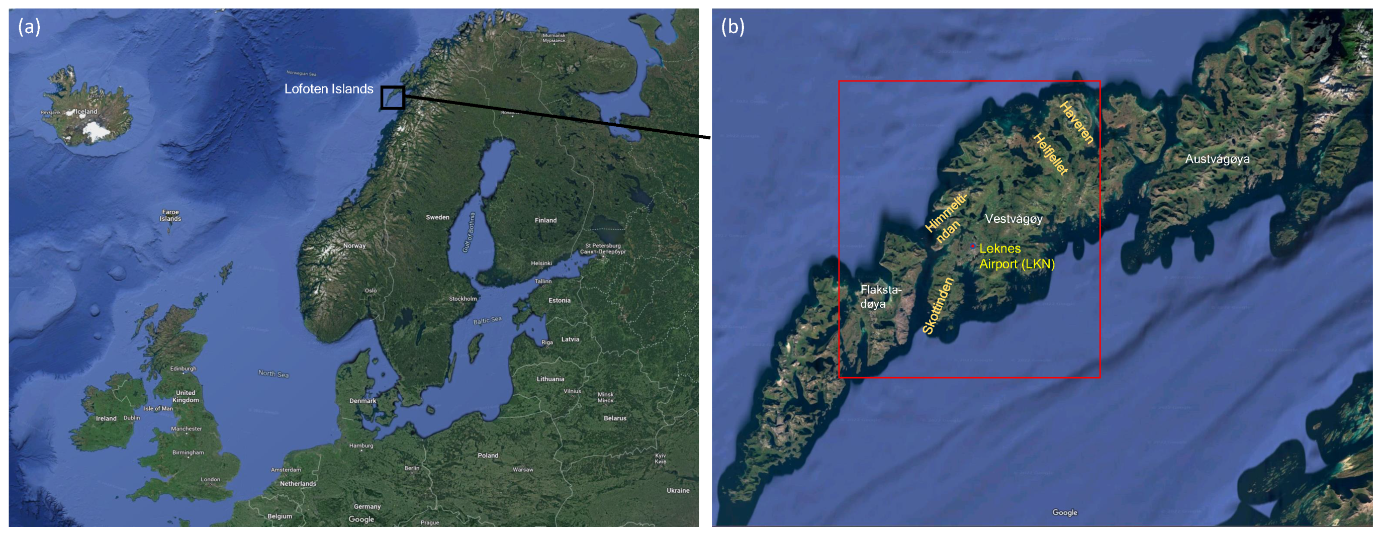
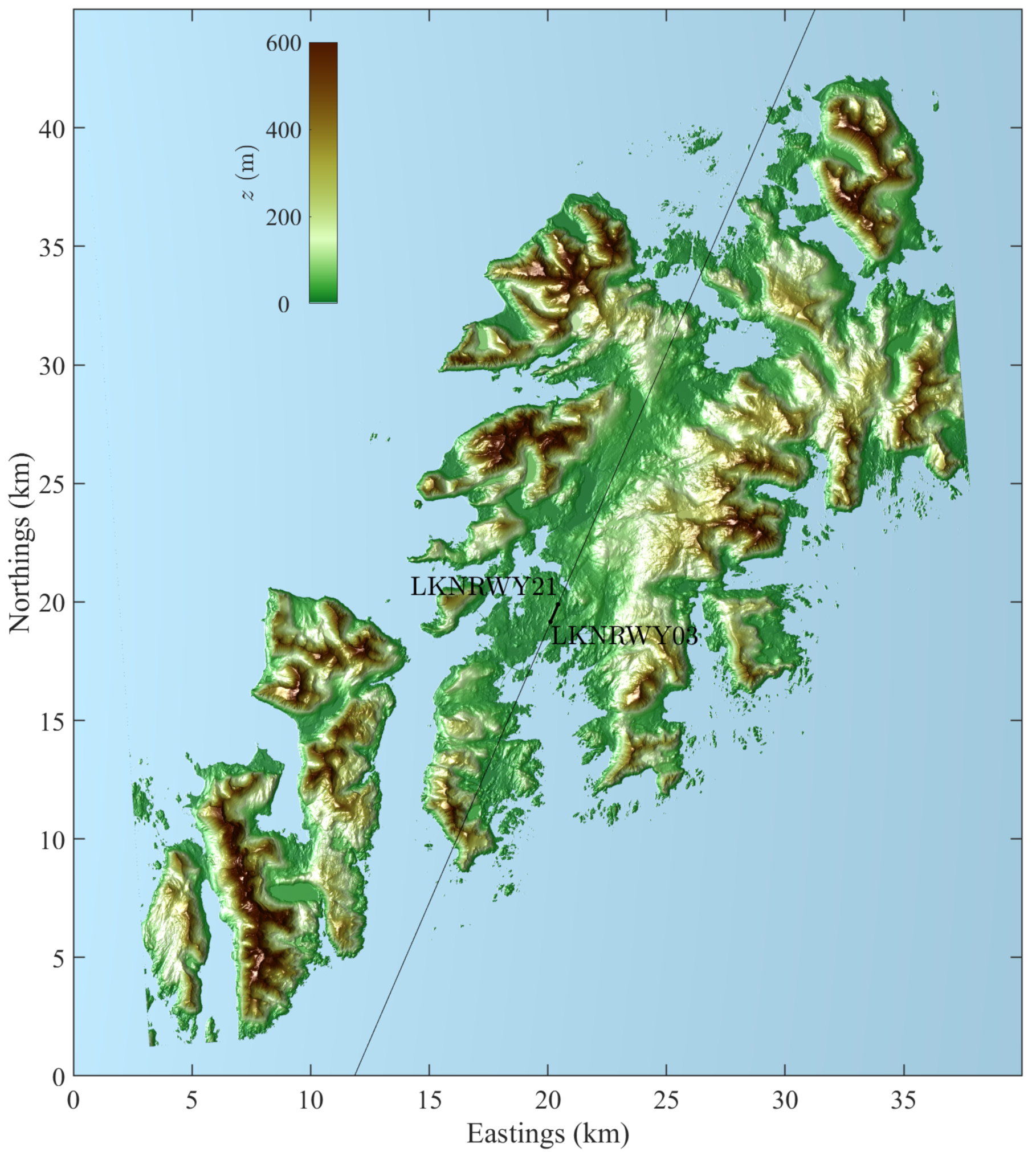
2. Study Area-Leknes, Lofoten Islands

Lofoten is an archipelago on the Northwestern coast of Norway, roughly located between 68 and 69${}^{°}$ N (see Figure 1a). It stretches over ca. 120 km in the SW-NE direction and is characterized by complex topography, with the highest peaks exceeding an elevation of 1000 m. The largest airport in the Lofoten islands is Leknes airport (IATA: LKN), which is located in the Southwestern part of the island of Vestvågøy at 68${}^{°}$09${}^{\prime }$09${}^{″}$ N 13${}^{°}$36${}^{\prime }$34${}^{″}$ E. Its runway lies approximately along the SSW-NNE direction (RWY03-RWY21) and has a length of 891 m, limiting it for regional operations with rather small aircraft, e.g., the De Havilland Canada models Dash-1 and Dash-8. Avinor, the operator of 44 state-owned airports in Norway, is a wholly-owned state limited company under the Norwegian Ministry of Transport and Communications, is recently investigating potential locations for a new airport on the Lofoten islands [33], allowing for direct access to the region with larger commercial aircraft. During this process, one year of observations with multiple scanning wind lidar systems has been performed at selected locations. Anticipating the future data availability of those measurements for research purposes, in particular for the comparison with our model simulations, we have chosen Leknes airport as our study area.

3. Materials and Methods

3.1. Simulation Setup

3.1.1. Simulation Model-PALM

Simulations for this work were performed with the PALM model version 6 revision 4579. PALM is an open-source, Fortran-based LES code, developed and maintained by the Institute of Meteorology and Climatology (IMUK) at the Leibniz University in Hannover, Germany. It is solving the spatially filtered, non-hydrostatic, incompressible Navier-Stokes equations using the Boussinesq approximation [34]. Advection terms are used in the prognostic equations and are realized by an upwind-based 5th-order differencing scheme [35] with a 3rd-order Runge-Kutta time-stepping scheme [36]. For parameterization of the eddies smaller than the grid spacing, PALM uses a subgrid-scale (SGS) model applying a 1.5th-order closure method following Deardorff 1980 [37], revised by Moeng and Wyngaard [38] and Saiki et al. [39]. This method is based on the hypothesis that the energy transport by SGS eddies is proportional to the local gradients of the mean quantities. For a detailed and general description of the PALM model, we refer to Maronga et al. [40,41]. PALM has been widely used in atmospheric boundary layer research for more than 20 years and numerous studies of the atmospheric boundary layer have been performed with this model [24,26].

3.1.2. Simulation Suite and Parameters

Based on the parameter set as described in

Table 1. Summary of main parameters used in the simulation for this study.

Name	Value
Grid resolution (dx, dy, dz)	50 m
Grid points	$800\times 900\times 80$
Simulated time	12 h
Number of timesteps	25,341
CPU cores	400
RAM allocated	32,768 MB
Initial surface sensible heat flux	$0.01{\mathrm{Kms}}^{-1}$
Zonal boundary condition	cyclic
Meridional boundary condition	cyclic
Vertical boundary condition	no-slip

, we conducted two sets of simulations for two geostrophic wind speeds of 10 (Set10) and 20 ms${}^{-1}$ (Set20). For each wind speed, simulations have been performed for 16 different wind directions (N, NNW, NW, WNW, W, WSW, SW, SSW, S, SSE, SE, ESE, E, ENE, NE, NNE), resulting in a total of 32 simulations. Every simulation output included hourly-averaged 3-D wind fields at every simulation hour. The TKE and wind distribution were analyzed for the whole computational domain.

3.1.3. Topography Data

The two-dimensional topography data was derived from the Norwegian Mapping Authority (Kartverket) [42,43]. The original dataset used the European Terrestrial Reference System 1989 (ETRS89) and the NN2000 altitude system. The datum was WGS89 and was in Digital Terrain Model with a grid resolution of 10 m (dtm10). The original data was block-averaged to fit the grid resolution of the corresponding LES simulation using MATLAB.

3.1.4. Domain and Boundary Conditions

The simulations used cyclic boundary conditions in both west-east (x) and south-north (y) directions. This requires that cells near the boundaries of the domain are fluid cells. As the Lofoten islands spread along the southwest-northeast direction, a truncation of the topography had to be performed to match this criterion for the western and eastern boundaries. Such a truncation has to be carefully chosen so that it doesn’t significantly affect the atmospheric flow near the LKN airport, as well as the numeric stability of integration at the boundaries of the domain. Ideally, the domain is chosen such that LKN is close to its centre, and the truncation of topography avoids steep gradients at the edge of the domain. What we need to avoid is that the potentially affected range in the downwind of the ridge on the boundary, expected to extend about 10 to 15 times of its altitude [44], will not disturb our area of interest around LKN. To achieve this, the horizontal size of the domain must be at least 2.5 times larger than this range in both directions [45,46]. Consequently, we chose for our study a rectangular simulation area between 13.17 and 14.04${}^{°}$ E in longitude, and 68.00 and 68.36${}^{°}$ N in latitude. The northern and southern boundaries lie completely in the ocean, the eastern boundary crosses the Lyndalsvatnet and the western boundary follows the Kåkersundet channel between the Flakstadøya and Moskenesøya islands. All boundaries were at least 19 km from LKN, and the steepest artificial edge by the truncation appears in the northwestern corner with an altitude of approximately 150 m. Thus, we are confident that our domain selection minimizes the effect of topography truncation. The scattered residuals and islands at the southwestern corner of the domain were also omitted. After the truncation, we end up with a rectangular box of $38.99\times 42.73{\mathrm{km}}^2$ with LKN located near the centre of the domain, see the red rectangle in Figure 1b. However, the west and east edges of this domain still contain solid cells, and the size of this domain (3899 × 4273) was not convenient for parallel computing, given the 400 cores we had on a high-performance computer (HPC) for simulations. Therefore, we added layers of fluid cells at all boundaries to fulfil the requirement of cyclic boundary conditions, as well as to make the number of grid points in every direction a multiple of 400.

In the vertical direction (z), the maximum height of the domain was set as 4 km. For the boundary conditions of potential temperature, a constant surface sensible heat flux was applied at the bottom, and the top sensible heat flux was calculated from the initial surface sensible heat flux and the initial potential temperature profile. For the boundary condition of horizontal velocity components, a no-slip condition was used at both the surface and the top of the domain. The final computational domain was chosen as the $40\times 45\times 4{\mathrm{km}}^3$ box shown in Figure 2.

3.1.5. Sensitivity Analysis

Although being an effective software to perform LES simulations, the expenses of computational power for such an extended domain in PALM are still extensively high (see

Table 2. Computational resource usage of one simulation in different grid resolutions. The simulated time was 12 h for each test.

Grid Resolution	Avg. Simulation Time	Avg. Memory Usage	Avg. Disk Write
25 m	20:21:56	493 GB	59 GB
50 m	01:15:36	141 GB	7 GB
100 m	00:17:22	111 GB	0.05 GB

). All the simulations were conducted on the HPC facility Fram, operated and maintained by the Norwegian research infrastructure services (NIRS). In order to balance simulation performance and computational expense, it is necessary that the grid resolution, as well as the overall simulation period, are carefully determined and optimized by sensitivity tests before conducting the full set of simulations. Therefore, we chose grid resolutions of 25, 50 and 100 m, and ran the simulation with otherwise identical parameters and topography data. The simulation time was initially set to 12 h to make sure the simulations have enough time to converge and stabilize. The corresponding results are shown in Figure 3 and indicate that the increase in velocity variances and TKE over time flattens distinctly at around 9 h. The simulations show, as expected, a clear increase in TKE (black lines) for decreasing grid spacing. Here the main improvement takes place for a refinement of the grid from 100 m to 50 m. A further decrease in grid spacing to 25 m improves the performance with respect to TKE resolution only marginally, consumes, however, nearly 20 times more computational resources. Based on those results we have chosen to perform the further simulations for 12 h with a horizontal and vertical grid resolution of 50 m.

3.2. Methodology

In our study, we investigate the three-dimensional characteristics of air-safety relevant BLT, with a particular focus on the conditions along the estimated glide paths during the final approach towards landing. The main proxy to represent the turbulence conditions in a computational region is the resolved TKE, i.e., the turbulent kinetic energy explicitly resolved and directly simulated by the model. At every hour in the PALM simulation, for a unit of air mass, hourly-averaged cardinal velocity components ($\overline{u},\overline{v},\overline{w}$) and squared cardinal velocity components ($\overline{u^2},\overline{v^2},\overline{w^2}$) were stored, and the hourly-mean resolved TKE was then calculated as:

$$TKE=\frac{1}{2}[(\overline{u^2}-{\overline{u}}^2)+(\overline{v^2}-{\overline{v}}^2)+(\overline{w^2}-{\overline{w}}^2)]$$

(1)

Note that the calculation in (1) is representing the resolved TKE per unit of air mass, so its dimension is $\mathrm{J}/\mathrm{kg}$, i.e., ${\mathrm{m}}^2{\mathrm{s}}^{-2}$.

The simplest meteorological variables considered most important for aviation safety are the F-factor [47], representing the wind shear ahead of the aeroplane, and the turbulence dissipation rate ${ϵ}^{1/3}$. These quantities are given by the Equations (2) and (3):

$$F={\overline{-\frac{c}{g}\frac{\partial u}{\partial x}+\frac{w}{c}}}^{l_f}=-\frac{c}{g{l}_f}[u(x+l_f/2-u(x-l_f/2)t]+\frac{{\overline{w}}^{l_f}}{c}$$

(2)

$${ϵ}^{1/3}\approx {\left(\frac{{\left(C_{\mu }^{1/2}K\right)}^{3/2}}{l_t}\right)}^{1/3}\approx 0.67K^{1/2}{l}_t^{-1/3}$$

(3)

here c is the flight path, g is the gravitational acceleration, $\mu$ is the wind component along the flight path, w is the vertical wind component, K is TKE, $l_t$ is turbulent length scale and $l_f$ is the minimum response distance in landing configuration, which is of the order of ∼500 m, corresponding to a time interval of about $t=O\left(7s\right)$. The coefficient $C_{\mu }$ has a value of approximately 0.09. A comprehensive review of this theory is given in Eldsvik et al. [48]. Regions prevailed by the conditions $F<-0.1$ and ${ϵ}^{1/3}>0.5{\mathrm{m}}^{2/3}{\mathrm{s}}^{-1}$ correspond to severe turbulence for commercial aircraft and represent potential danger [49]. These conditions are easily met when $K^{1/2}>3{\mathrm{ms}}^{-1}$, so we chose 9 ${\mathrm{m}}^2{\mathrm{s}}^{-2}$ as the TKE threshold to distinguish locations with high turbulence risk in our study.

In the investigation of aviation safety, we aim to analyze the potential risk a pilot might encounter during the final approach and take-off. However, the realistic strategies differ in terms of weather and visibility conditions, especially for airports near complex terrain. As a simplified model, we defined a 3-degree aircraft glide slope at both ends of the LKN runway to represent the approximate trajectory of an aircraft in our study [50]. In terms of aircraft landing, this model is very close to the realistic landing approach. For take-off, this model is less precise as the pitch slope of the aircraft varies from 3–12 degrees depending on the size of the aircraft, but still makes sense in analyzing the altitudes where high turbulence risk occurs near the airport. In addition, an aircraft during the start of take-off is considerably less vulnerable to the effect of terrain induced turbulence.

Based on this flight path model, turbulence hazard risks were then analyzed for all simulations. For each scenario, data selection along the flight path was done as follows: (1) coordinates of the intersections between the glide path and all the south-north surfaces were derived, (2) for each intersection, 4 adjacent grid points were collected as sample points. The sample points were then categorized according to TKE values and locations (RWY03 or RWY21), and the frequency of grid cells exceeding the TKE threshold was calculated to quantify the overall potential of turbulence hazard in each scenario.

4. Results

The main part of this study is dedicated to the spatial characterization of potentially dangerous situations of terrain induced BLT, dependent on wind speed and wind direction. In the following, we will present and discuss the simulation results of resolved TKE in the form of horizontal cross-sections at different altitude levels over the whole domain, the vertical cross-section defined by the orientation of the existing runway of LKN, and spatial profiles of TKE along the aircraft glide path during landing. To simplify the notations, in the remainder of the manuscript, the different model runs will be identified by the abbreviation of the wind direction, followed by the number of the corresponding wind speed. For example, the simulation with a 20 ms${}^{-1}$ northwestern geostrophic wind is abbreviated as “NW20”.

4.1. Atmospheric Stratification

In PALM, the atmospheric stratification is determined by the wind speed and the sensible heat flux at the bottom surface [51]. To investigate its effect on the turbulence simulations, we selected 3 heat flux cases: (a) 0.01 Kms${}^{-1}$, indicating near-neutral conditions; (b) 0.1 Kms${}^{-1}$ representing moderately convective conditions and (c) 0.3 Kms${}^{-1}$ for strongly convective conditions. Otherwise identical simulations of these 3 scenarios were performed for a geostrophic wind of 20 ms${}^{-1}$ from Northwest (NW) and the resulting profiles of the resolved TKE along the glide path are presented in Figure 4. The profiles show highly variable TKE values including several terrain induced peaks, with three of them exceeding the threshold of 9 ${\mathrm{m}}^2{\mathrm{s}}^{-2}$. The maximum peak, in a distance between 5 and 10 km from the airport, reaches even above 25 ${\mathrm{m}}^2{\mathrm{s}}^{-2}$, indicating severe BLT conditions induced by the terrain. However, the profiles for the different stability conditions are very similar in shape and absolute value and indicate that atmospheric stability plays only a secondary role in the creation of terrain-induced TKE. Thus we have chosen to only use the heat flux value of 0.01 Kms${}^{-1}$ further on in this study.

4.2. Turbulence Characteristics as Function of Wind Speed and Direction

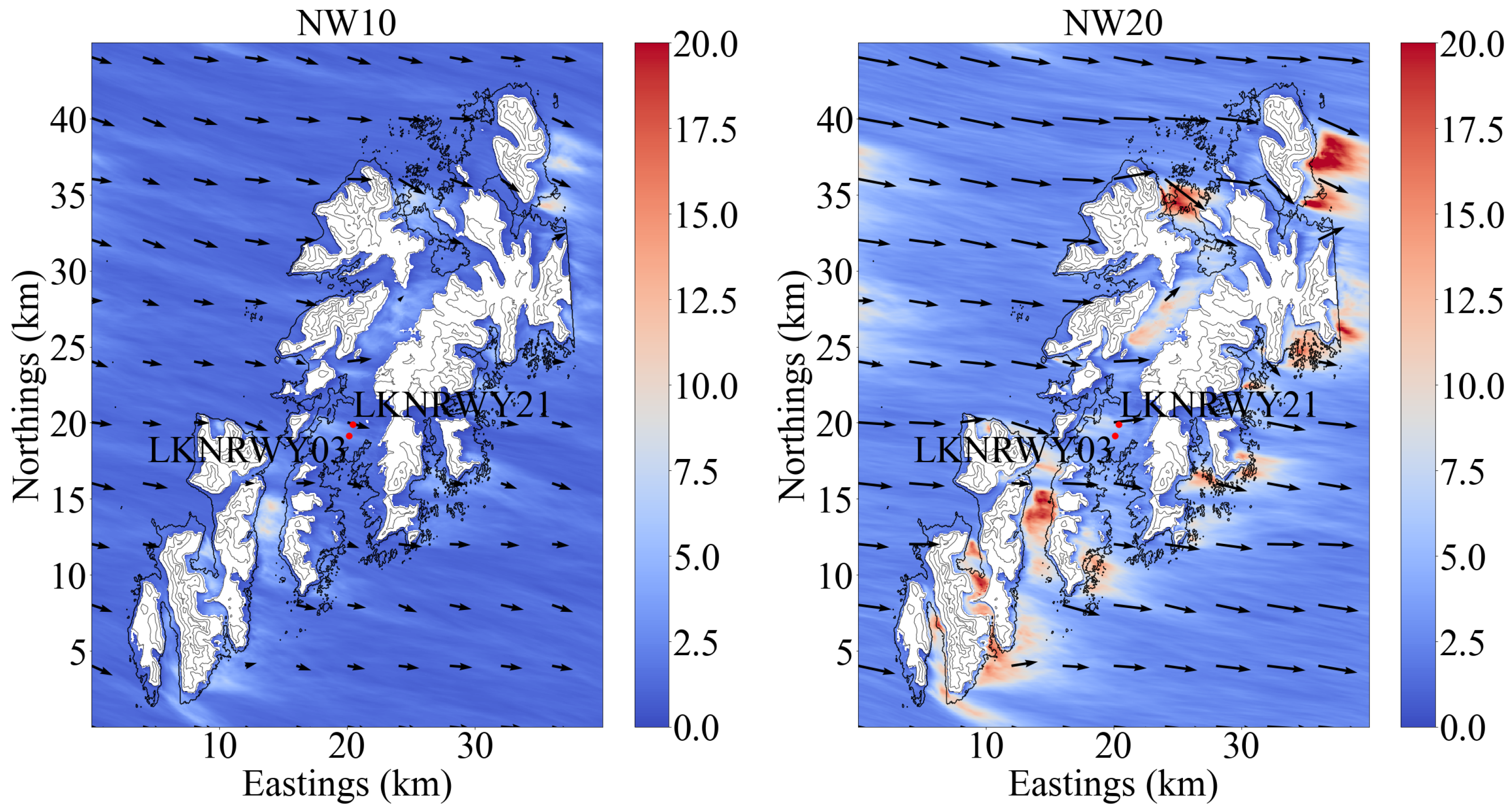
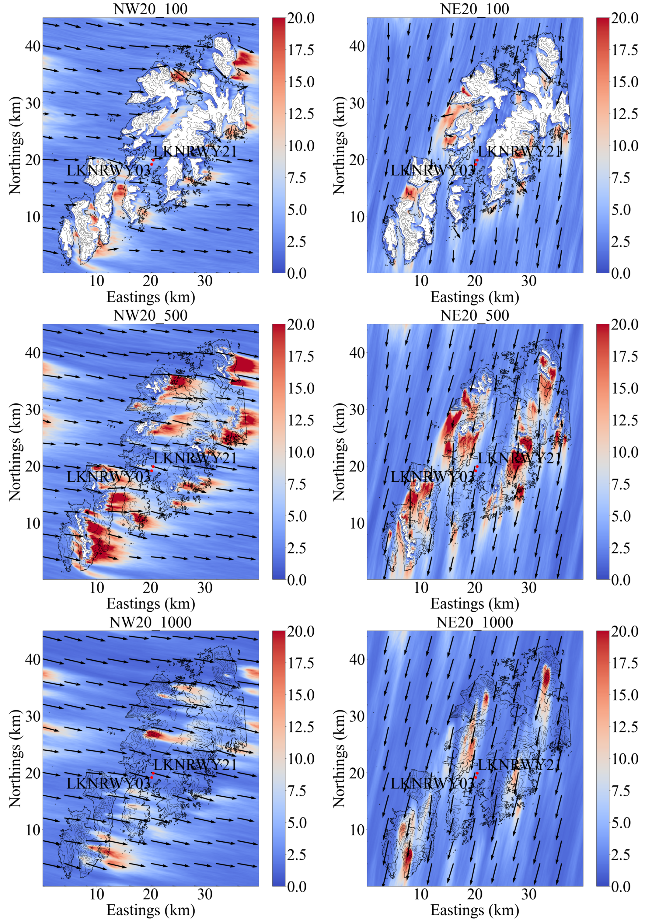
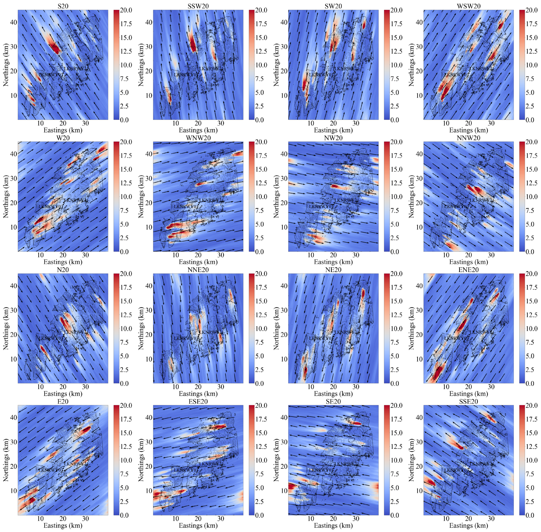
4.2.1. Horizontal Cross-Sections

The horizontal wind field and resolved TKE field were analyzed for the complete area of interest at the three heights of 100 m, indicating the layer LLT appears, 500 m and 1000 m, roughly the level of the highest mountain tops. The key features of selected simulations are described in the following section, while the corresponding plots of all simulations are available in the Appendix A (Figure A1 and Figure A2).

Figure 5 presents the results for the simulations with a geostrophic wind from NW of 10 ms${}^{-1}$ and 20 ms${}^{-1}$ (cases NW10, left panel and NW20, right panel) at an altitude of 100 m. NW10 shows over the whole model domain considerably lower TKE values than NW20, indicated by the darker blue colour. There is an indication of weak terrain induced turbulence in the lee of the mountains, the TKE threshold of 9 ${\mathrm{m}}^2{\mathrm{s}}^{-2}$ is, however, hardly reached or exceeded in this run. The simulations for NW20 show, in contrast, distinct maxima in the TKE field that exceed the threshold nearly everywhere on the lee side of the topography. Those patches of heavy terrain-induced turbulence extend typically for at least 5 km downwind from the initiating mountain ridges, before gradually dissipating. No significant signal was found near the airport runway in either case, and the turbulence condition in the valley of Vestvagøy was only moderate. This indicates a relatively low probability for an aircraft experiencing LLT related safety issues at this level.

One feature worth noticing in the horizontal cross-section plots is the turn of wind direction relative to the geostrophic wind. In NW20, the wind direction at 100 m height is more or less purely west, indicating a counter-clockwise turn of 30–40${}^{°}$ from its geostrophic start value. This can be explained by the effect of surface friction within the Ekman layer, resulting in ageostrophic and cross-isobaric winds inside the ABL.

Figure 6 presents exemplary results for the simulations with a 20 ms${}^{-1}$ geostrophic wind from NW (left column, NW20) and NE (right column, NE20) for three different ABL levels of 100 m (top plots), 500 m (center plots), and 1000 m (bottom plots). The full set of simulations for the three altitude levels can be found in Appendix A (Figure A2, Figure A3 and Figure A4). The NW case shows in general overall slightly higher TKE levels and correspondingly also larger areas affected by strong turbulence above the TKE threshold level. This indicates that the effect of the orientation of the topography with respect to the wind direction plays an important role. The highest TKE levels for both wind directions are observed in the cross-sections at 500 m altitude, more or less corresponding to the average altitude of turbulence inducing terrain features in the free flow. At 1000 m only the highest peaks can contribute to corresponding disturbances, and their abundance is therefore considerably reduced. Compared to the 100 m level, the higher cross-sections indicate also a clearly increased downwind extension of the turbulent patches, often exceeding 10 km from their origin.

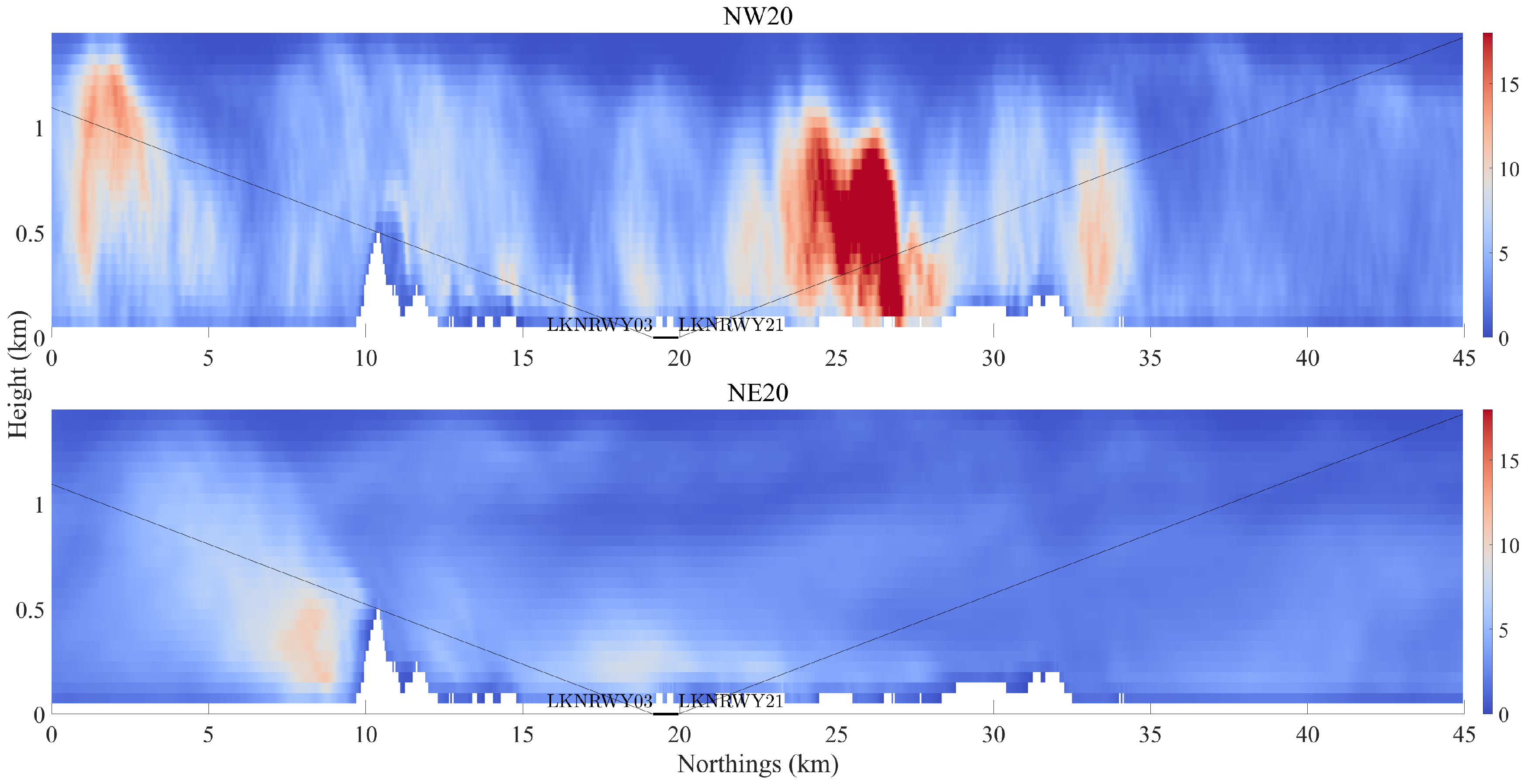
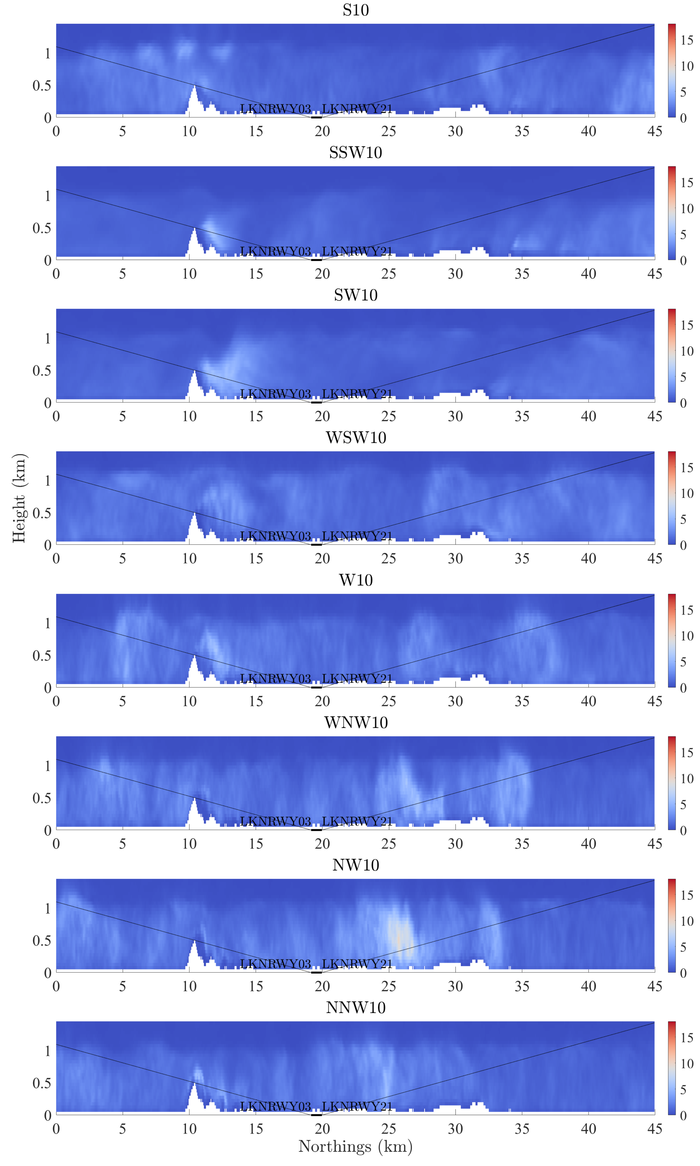
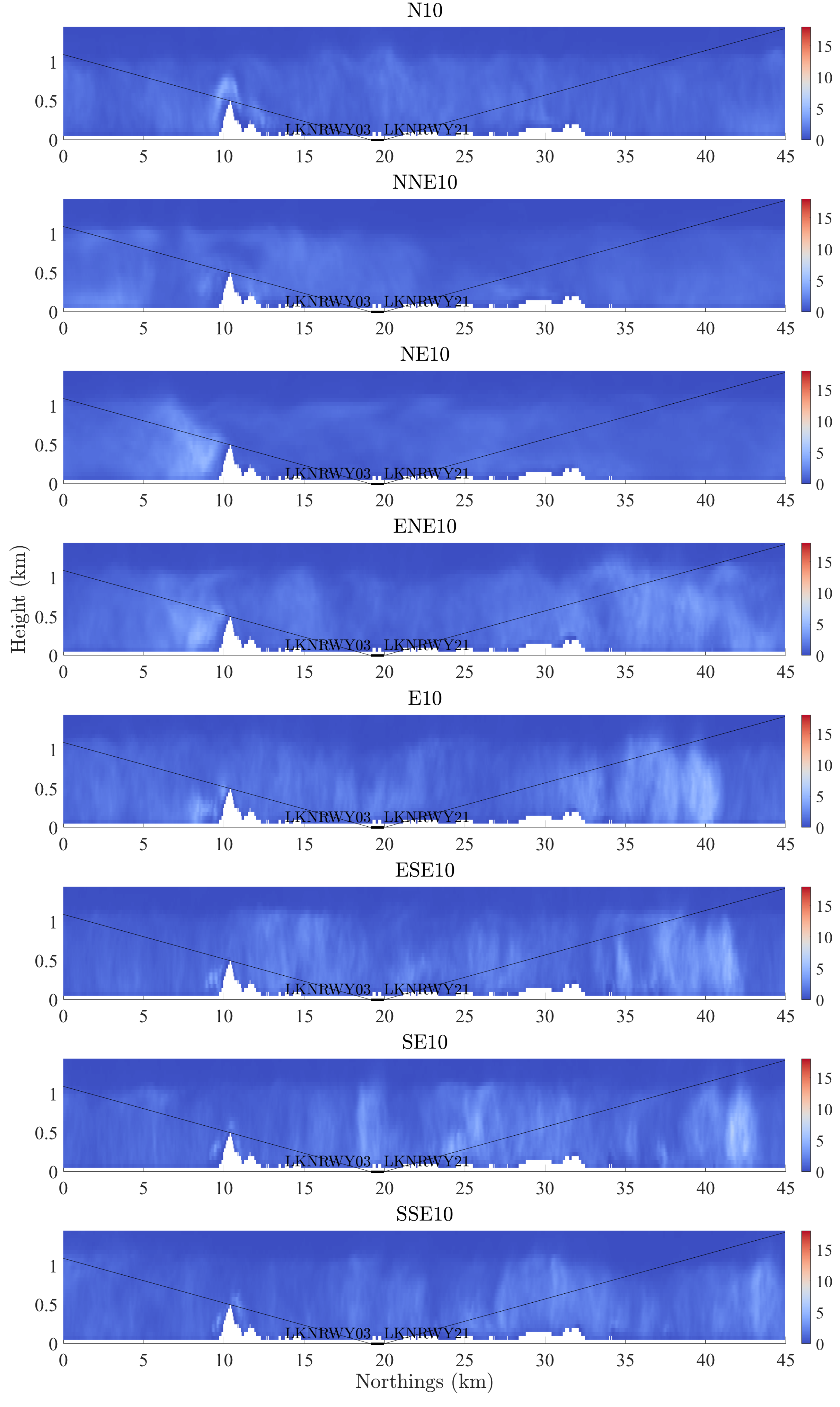
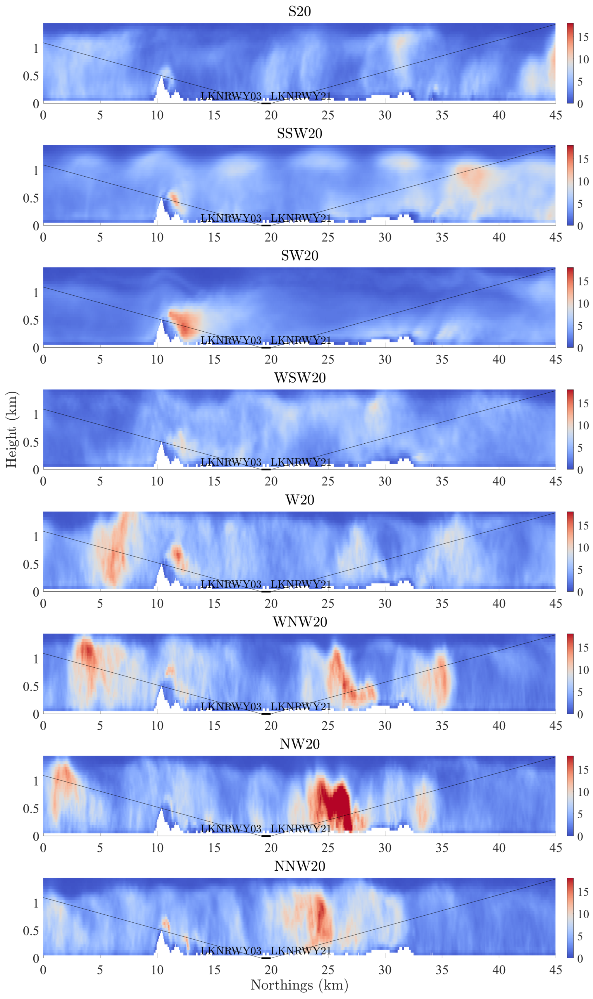
4.2.2. Vertical Cross Sections

The vertical resolved TKE field was also analyzed at the vertical cross-section in the direction of the LKN runway from the surface to 1500 m. Plots of all simulations for 10 ms${}^{-1}$ and 20 ms${}^{-1}$ are available in Appendix A (Figure A5 and Figure A6). Figure 7 illustrates the distributions of TKE for the NW20 and NE20 cases, the glide slopes are indicated by the thin black lines. In correspondence with the findings presented in Figure 6, we can observe a clear discrepancy in the amount of resolved TKE between these two cases. In NW20, there are three turbulence hot spots intersecting with the glide slope, one in the direction of RWY03, and the two others along RWY21. The maximum is observed at a distance of approximately 5km from LKNRWY21, and its intersection with the glide slope is at around 400 m height. By referring to the topography, we can associate this maximum with the hills next to LKN to the north. This maximum in NW20 extends to around 1000 m and quickly fades until above 1200 m, in correspondence with the initializing peak Himmeltindan of 982 m height. In contrast, the general situation of resolved TKE in NE20 is low to moderate, with only one area of slightly enhanced TKE at about 10 km south of LKNRWY03, located in the lee of the hills next to LKN in the south. A possible explanation for such discrepancy is the difference of orographic form drag the flow experiences [52,53], dependent on the orientation of the turbulence initiating terrain relative to the wind direction. In addition are the upstream flow conditions different for the two chosen wind directions. For NW20, wind travels only above the ocean before reaching the hills, thus most of its kinetic energy is preserved, providing more energy available for generating turbulent eddies. For NE20, on the other hand, the wind has crossed over tens of kilometres of mountainous area when reaching the hill, and parts of its kinetic energy has been dissipated due to frictional effects. This general difference in wind speed can also be observed in Figure 6, where the leeward created TKE in NE20. With significantly reduced wind speed, the TKE generated in the leeward becomes less accordingly.

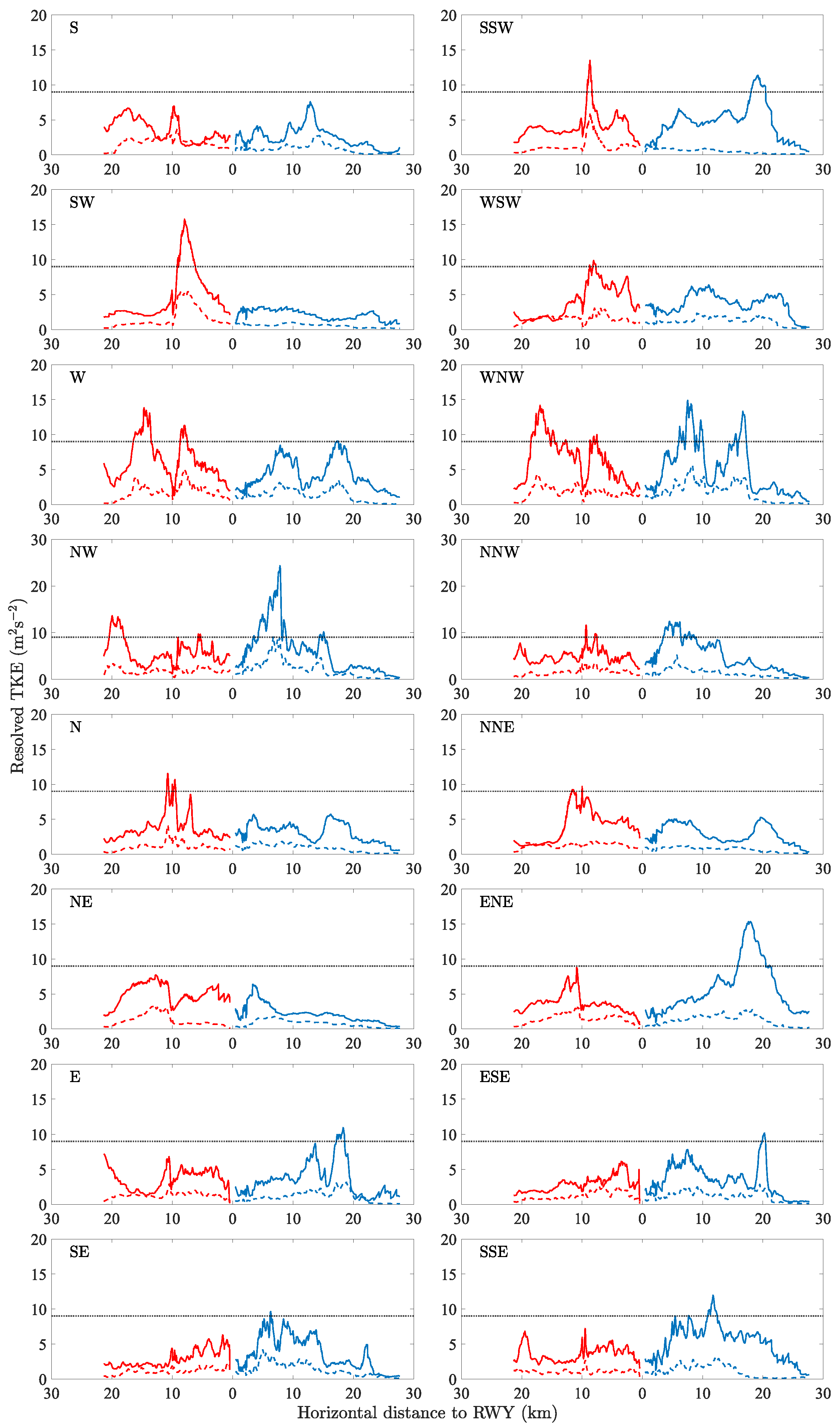
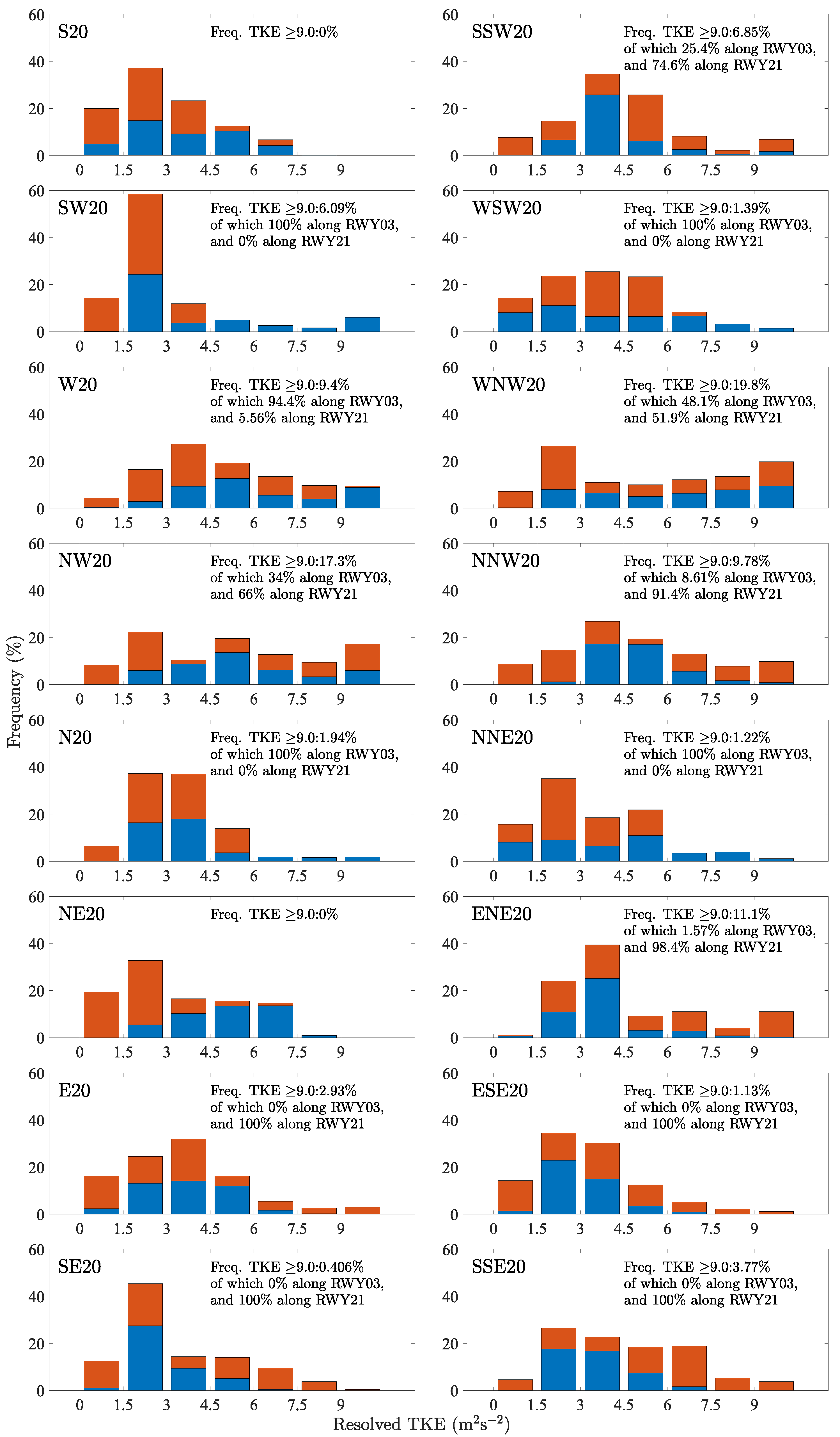
4.3. Aviation Safety Risk Analysis on the Glide Slope

For an estimation of the potential of turbulence encounters in flight, we present spatial TKE profiles along the slanted gliding path. As explained before, we have in this study chosen a hypothetical constant glide angle for this purpose. With the availability of more detailed flight route information for start and landing in the future, our method can be easily adapted. Figure 8 shows the turbulence distribution along the glide slope for all simulations, illustrating the potential turbulence risks and locations an aircraft might encounter during start and landing. Dashed lines correspond to the simulations with a geostrophic wind speed of 10 ms${}^{-1}$ (set10), solid lines to ones of 20 ms${}^{-1}$ (set20). The different colours indicate the direction of the two glide paths originating from LKN airport, in blue the one towards NNE (LKNRWY03) and in red the one towards SSW (LKNRWY21). For set10 the threshold of 9 ${\mathrm{m}}^2{\mathrm{s}}^{-2}$ is never exceeded for any of the 16 different wind directions. Consequently, air safety related issues due to terrain induced BLT are not to be expected for wind speeds below and around 10 ms${}^{-1}$. For most of the wind directions of set20, with exception of two (S and NE), one or several peaks in TKE exceed the threshold, giving a clear indication that terrain induced turbulence provokes a common and considerable aviation risk near LKN when the wind speed approaches 20 ms${}^{-1}$. Fortunately, none of those peaks are situated in the near-surface region close to the runway, meaning that it is not likely for an aircraft to encounter strong turbulence at very low altitudes close to touchdown.

For a quantitative comparison of the related risks, a statistical analysis of the turbulence conditions along the glide slope was performed, following the methodology described in Section 3.2. The probability of high turbulence risk is expressed by the frequency of occurrence of extreme TKE values along the glide path, calculated as the ratio of grid cells exceeding the 9 m${}^2$s${}^{-2}$ threshold to all grid cells along the glide path. The results of this analysis are summarized in Figure 9. Among the 16 cases in set20, the most turbulent one is NW20, with 17.3%, while the least turbulent case is NE20, which doesn’t have a single high-risk case. The highest peak in the RWY21 direction is also found in NW20, which is the maximum of above 25 m${}^2$s${}^{-2}$ we discussed in Section 4.2.2. The highest TKE value in the RWY03 direction is found in SW20, which is related to the hills in the south of LKN. By cross-comparing the profiles, we notice that the cases under adjacent geostrophic wind directions share similar features in the locations and magnitude of TKE peaks, so it is logical to discuss them in groups.

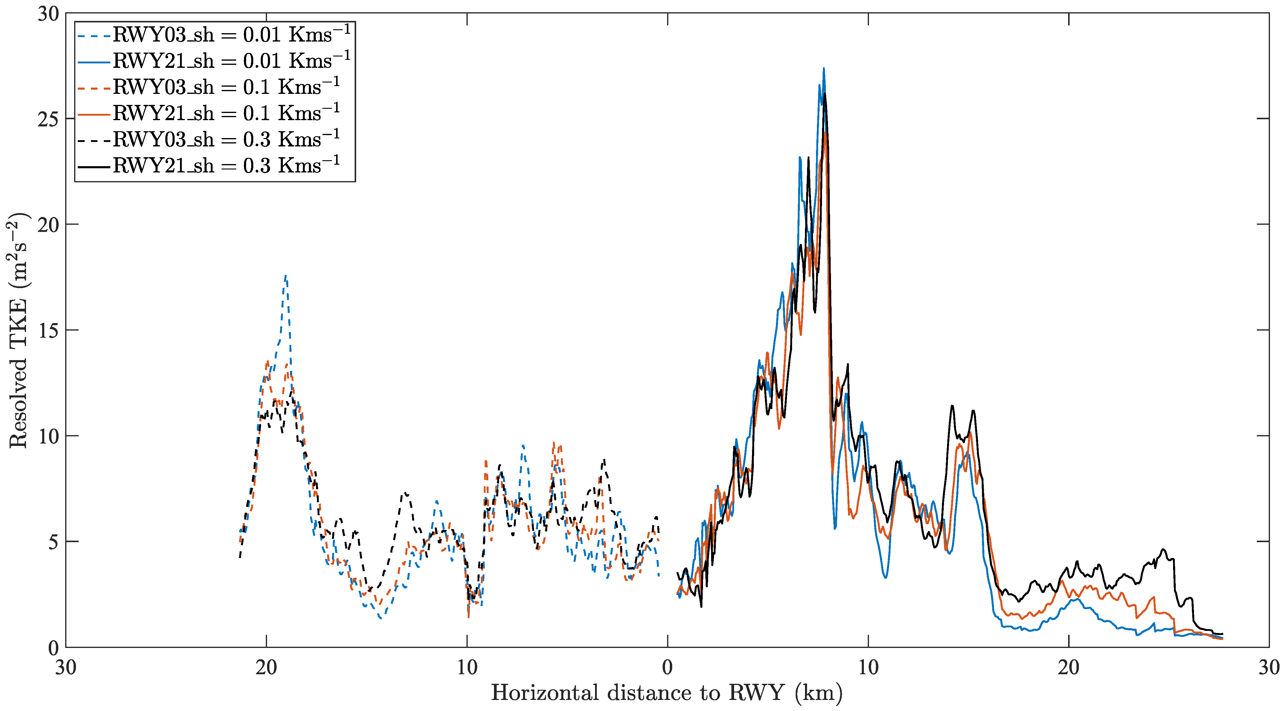
• Southwesterly group (S20, SSW20, SW20, WSW20): The overall resolved TKE condition of this group is moderate, with a high turbulence probability of 3.6%. For the direction of RWY03, main peaks are observed in the lee of Skottind. For RWY21, only one high-risk area is found in SSW20.
• Northwesterly group (W20, WNW20, NW20, NNW20): This group reports considerably more turbulence hot spots than the others, with a high turbulence probability of 14.1%. According to the profiles, there are two common hot spots along the RWY03 slope, and another two along the RWY21 slope. If we assume an aircraft is approaching along the RWY03 slope, it will first encounter intensive turbulence at approximately 750 m altitudes. This hot spot is located at the lee of the mountains on Flakstadøya. The mountains there run north to south, maximizing the blockage effect on northwesterly winds, and, as a result, generating high turbulence levels. The aircraft will cross high turbulence again at about 400 m in altitude. As discussed in Section 4.2, this hot spot is related to the mountains to the south of LKN.
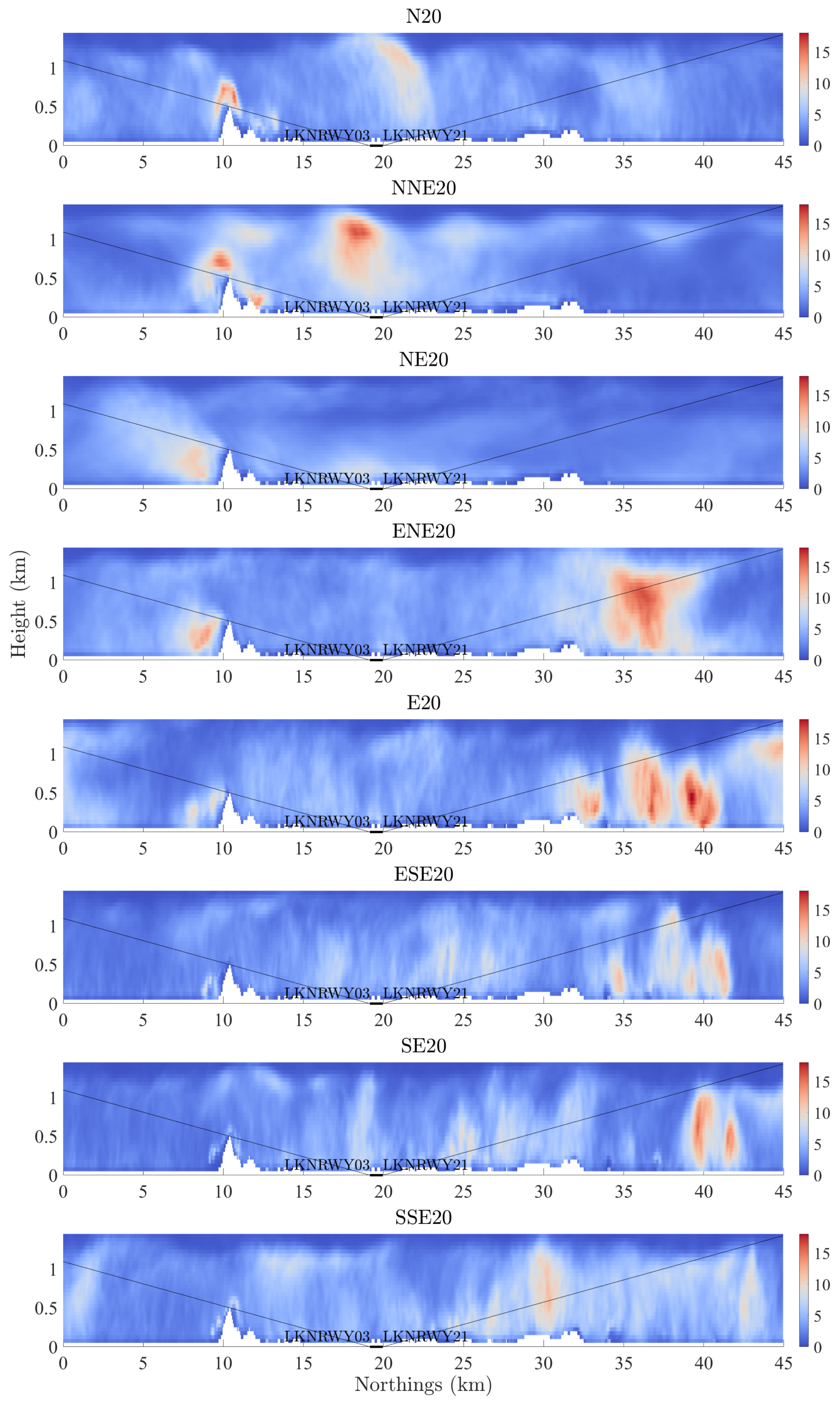
• Northeasterly group (N20, NNE20, NE20, ENE20): The high turbulence risk of this group is, 3.6%, again, moderate. Unlike the other groups, whose extreme values distribute relatively evenly, most of the extremes in this group are found in the major peak of ENE20. This peak stands out at about 20 km distance from RWY21, located above two lakes (Urvatnet and Steirapollen), situated between the mountains Helfjellet and Haveren. As discussed in Section 4.2.1, the wind field here turns northeasterly, maximizing the interference with Haveren. As a result, high turbulence levels are induced in the downwind region. The mechanism and wind setting of NE20 is quite similar, but the statistics yield results with huge contrast. By investigating the turbulence distribution for the whole domain, one can observe that the total amount of resolved TKE between NE20 and ENE20 is rather similar. However, due to the slight shift in wind direction, the turbulence hot spot induced by Haveren, moves slightly southeastwards to the lake Alstadpollen, making it undetectable in the cross-section along the LKN runway.
• Southeasterly group (E20, ESE20, SE20, SSE20): This group is least overall least exposed to turbulence risks among the four groups, with a high turbulence probability of 2.1%. There are no shared peak locations among the group members, instead, various extreme values (with relatively low magnitude) spread in the region 10–20 km away from RWY21, i.e., the northeastern part of the main valley on the Vestvågøya island. The potential reason this group experiences the least turbulence risk is the fact that the topography on the southeastern side of Vestvågøya is lower and gentler than its northwestern counterpart, but spread more continuously. Therefore, as the easterly winds in this group interfere with the mountains, turbulent eddies are induced in a larger area but with overall lower TKE intensity.

5. Conclusions and Outlook

This study investigates the turbulence conditions in the surroundings of the existing Leknes airport in the Lofoten islands. We studied the terrain-induced turbulence in the atmospheric boundary layer and performed a turbulence risk analysis on an idealized aircraft trajectory with respect to different geostrophic wind speeds and directions. To achieve these goals, a suite of simulation runs was carried out using the LES model PALM, based on a high-resolution topography dataset near the LKN airport in the Lofoten islands. Based on initial parametric sensitivity studies we have finally chosen a grid spacing of 50 m and a simulation time of 12 h for a suite of model simulations for 16 different wind directions and two geostrophic wind speeds of 10 ms${}^{-1}$ and 20 ms${}^{-1}$. The results show that PALM can properly simulate the turbulent flows for air safety related investigations in an extended domain with high resolution at an acceptable computational expense.

According to the simulation results of the wind field and turbulence in the whole domain, we demonstrated that the topographically-induced turbulence occurs in the lee of steep mountains and ridges. Those terrain-induced turbulence patterns extend typically 5 to 10 km downstream, with an indication of a slight increase in this extension with altitude. The highest TKE levels are observed in the middle of the ABL around 500 m altitude, more or less corresponding to the level of turbulence inducing terrain features in the free flow.

A turbulence risk analysis along idealized flight trajectories shows that the turbulence risk conditions are substantially determined by the wind conditions and their interaction with the topography. With respect to wind speed, the results indicate that for a geostrophic flow below 10 ms${}^{-1}$, the risk of aviation critical, terrain-induced BLT, is rather low in the vicinity of LKN. At 20 ms${}^{-1}$ the situation has completely changed and the aviation critical threshold of 9 m${}^2$s${}^{-2}$ is exceeded for 14 out of 16 of the investigated wind directions. Two main factors influence the observed directional dependency of the turbulence risk, one being the orientation of the topography with respect to the wind direction, and the fetch, i.e., the average upstream surface characteristics. Turbulent eddies in the lee form are particularly efficient when the flow intersects almost perpendicularly with the steep topography. The orographical form drag also plays an important role, as it affects the average wind speed of the upstream flow. The main topographic features are SW to NE oriented, with an average altitude decreasing from NW to SE. However, the southwestern mountains, mainly on Flakstadøya, run north to south. From the profiles and statistics we observed, for the southwestern glide slope RWY03, the highest turbulence risk occurs under westerly winds, and for the northeastern glide slope RWY21, the highest turbulence risk is associated with northwesterly wind.

This study presents a novel methodology as it uses for the first time a systematic LES modelling approach for the investigation of the turbulence characteristics for two geostrophic wind speeds and 16 different wind directions. Although the simulations already cover a considerable range of relevant meteorological conditions for the operation of a future airport, this study comprises still a limited subset of cases, in particular for higher wind speeds from critical wind directions. This is, however, beyond the scope of this proof-of-concept study. It should also be emphasized that the choice of aircraft trajectories in this study is rather idealistic. Nevertheless, it already provides a very good indication of the aviation relevant BLT risks in the vicinity of LKN. The design of our method allows, in addition, for an easy adaptation as soon as more detailed flight route information for take-off and landing will be available in the future.

A next natural step in the extension of this study would be a case study based comparison of the LES results with remotely sensed wind fields, e.g., collected by scanning Doppler-lidars [26,54] or acoustic soundings [55] in the area. This could be accomplished by either getting access to an already existing data set from Avinor, or by designing and performing a new and targeted measurement campaign that would, in the context of instrument placement and scanning patterns, highly benefit from the now available LES data set.

References

1. Sharman, R.; Lane, T. (Eds.) Aviation Turbulence; Springer International Publishing: Cham, Switzerland, 2016. [Google Scholar] [CrossRef]
2. Gultepe, I.; Sharman, R.; Williams, P.D.; Zhou, B.; Ellrod, G.; Minnis, P.; Trier, S.; Griffin, S.; Yum, S.S.; Gharabaghi, B.; et al. A Review of High Impact Weather for Aviation Meteorology. Pure Appl. Geophys. 2019, 176, 1869–1921. [Google Scholar] [CrossRef]
3. WMO. Aviation|Hazards|Turbulence and Wind Shear. Available online: https://community.wmo.int/activity-areas/aviation/hazards/turbulence (accessed on 1 March 2022).
4. Stull, R.B. An Introduction to Boundary Layer Meteorology; Springer: Dordrecht, The Netherlands, 1988. [Google Scholar] [CrossRef]
5. Sharman, R.D.; Trier, S.B.; Lane, T.P.; Doyle, J.D. Sources and dynamics of turbulence in the upper troposphere and lower stratosphere: A review. Geophys. Res. Lett. 2012, 39. [Google Scholar] [CrossRef]
6. Trier, S.B.; Sharman, R.D.; Lane, T.P. Influences of Moist Convection on a Cold-Season Outbreak of Clear-Air Turbulence (CAT). Mon. Weather Rev. 2012, 140, 2477–2496. [Google Scholar] [CrossRef]
7. Kim, J.H.; Chun, H.Y. Statistics and Possible Sources of Aviation Turbulence over South Korea. J. Appl. Meteorol. Climatol. 2011, 50, 311–324. [Google Scholar] [CrossRef]
8. Doyle, J.D.; Jiang, Q.; Smith, R.B.; Grubišić, V. Three-dimensional characteristics of stratospheric mountain waves during T-REX. Mon. Weather Rev. 2011, 139, 3–23. [Google Scholar] [CrossRef]
9. Lane, T.P.; Sharman, R.D.; Trier, S.B.; Fovell, R.G.; Williams, J.K. Recent Advances in the Understanding of Near-Cloud Turbulence. Bull. Am. Meteorol. Soc. 2012, 93, 499–515. [Google Scholar] [CrossRef]
10. Hon, K.K.; Chan, P.W. Alerting of hectometric turbulence features at Hong Kong International Airport using a short-range LIDAR. Meteorol. Appl. 2020, 27, 1–10. [Google Scholar] [CrossRef]
11. Smagorinsky, J. General circulation experiments with the primitive equations: I. The basic experiment. Mon. Weather Rev. 1963, 91, 99–164. [Google Scholar] [CrossRef]
12. van Heerwaarden, C.C.; Mellado, J.P. Growth and Decay of a Convective Boundary Layer over a Surface with a Constant Temperature. J. Atmos. Sci. 2016, 73, 2165–2177. [Google Scholar] [CrossRef]
13. Rai, R.K.; Berg, L.K.; Pekour, M.; Shaw, W.J.; Kosovic, B.; Mirocha, J.D.; Ennis, B.L. Spatiotemporal Variability of Turbulence Kinetic Energy Budgets in the Convective Boundary Layer over Both Simple and Complex Terrain. J. Appl. Meteorol. Climatol. 2017, 56, 3285–3302. [Google Scholar] [CrossRef]
14. Huang, J.; Bou-Zeid, E. Turbulence and Vertical Fluxes in the Stable Atmospheric Boundary Layer. Part I: A Large-Eddy Simulation Study. J. Atmos. Sci. 2013, 70, 1513–1527. [Google Scholar] [CrossRef]
15. Sullivan, P.P.; Weil, J.C.; Patton, E.G.; Jonker, H.J.J.; Mironov, D.V. Turbulent Winds and Temperature Fronts in Large-Eddy Simulations of the Stable Atmospheric Boundary Layer. J. Atmos. Sci. 2016, 73, 1815–1840. [Google Scholar] [CrossRef]
16. van der Linden, S.J.A.; Edwards, J.M.; van Heerwaarden, C.C.; Vignon, E.; Genthon, C.; Petenko, I.; Baas, P.; Jonker, H.J.J.; van de Wiel, B.J.H. Large-Eddy Simulations of the Steady Wintertime Antarctic Boundary Layer. Bound. Layer Meteorol. 2019, 173, 165–192. [Google Scholar] [CrossRef]
17. Bechmann, A.; Sørensen, N.N.; Berg, J.; Mann, J.; Réthoré, P.E. The Bolund Experiment, Part II: Blind Comparison of Microscale Flow Models. Bound. Layer Meteorol. 2011, 141, 245–271. [Google Scholar] [CrossRef]
18. Liu, Z.; Cao, S.; Liu, H.; Ishihara, T. Large-Eddy Simulations of the Flow Over an Isolated Three-Dimensional Hill. Bound. Layer Meteorol. 2019, 170, 415–441. [Google Scholar] [CrossRef]
19. Vollmer, L.; Steinfeld, G.; Heinemann, D.; Kühn, M. Estimating the wake deflection downstream of a wind turbine in different atmospheric stabilities: An LES study. Wind Energy Sci. 2016, 1, 129–141. [Google Scholar] [CrossRef]
20. Martínez-Tossas, L.A.; Churchfield, M.J.; Yilmaz, A.E.; Sarlak, H.; Johnson, P.L.; Sørensen, J.N.; Meyers, J.; Meneveau, C. Comparison of four large-eddy simulation research codes and effects of model coefficient and inflow turbulence in actuator-line-based wind turbine modeling. J. Renew. Sustain. Energy 2018, 10, 033301. [Google Scholar] [CrossRef]
21. Abkar, M.; Porté-Agel, F. Influence of atmospheric stability on wind-turbine wakes: A large-eddy simulation study. Phys. Fluids 2015, 27, 035104. [Google Scholar] [CrossRef]
22. Taylor, A.C.; Beare, R.J.; Thomson, D.J. Simulating Dispersion in the Evening-Transition Boundary Layer. Bound. Layer Meteorol. 2014, 153, 389–407. [Google Scholar] [CrossRef]
23. Resler, J.; Eben, K.; Geletič, J.; Krč, P.; Rosecký, M.; Sühring, M.; Belda, M.; Fuka, V.; Halenka, T.; Huszár, P.; et al. Validation of the PALM model system 6.0 in a real urban environment: A case study in Dejvice, Prague, the Czech Republic. Geosci. Model Dev. 2021, 14, 4797–4842. [Google Scholar] [CrossRef]
24. Knigge, C.; Raasch, S. Large-Eddy Simulation on the Influence of Buildings on Aircraft during Take Off and Landing. Available online: https://www.researchgate.net/publication/268648516_Large-eddy_simulation_on_the_influence_of_buildings_on_aircraft_during_take_off_and_landing (accessed on 18 April 2022).
25. Bergot, T.; Escobar, J.; Masson, V. Effect of small-scale surface heterogeneities and buildings on radiation fog: Large-eddy simulation study at Paris-Charles de Gaulle airport. Q. J. R. Meteorol. Soc. 2015, 141, 285–298. [Google Scholar] [CrossRef]
26. Chan, P.W.; Lai, K.K.; Li, Q.S. High-resolution (40 m) simulation of a severe case of low-level windshear at the Hong Kong International Airport—Comparison with observations and skills in windshear alerting. Meteorol. Appl. 2021, 28, 1–25. [Google Scholar] [CrossRef]
27. Liu, X.; Abà, A.; Capone, P.; Manfriani, L.; Fu, Y. Atmospheric Disturbance Modelling for a Piloted Flight Simulation Study of Airplane Safety Envelope over Complex Terrain. Aerospace 2022, 9, 103. [Google Scholar] [CrossRef]
28. WMO. Aircraft Meteorological Data Relay (AMDAR) Reference Manual; Technical Report 958; World Meteorological Organization (WMO): Geneva, Switzerland, 2003. [Google Scholar]
29. Sharman, R. Nature of Aviation Turbulence. In Aviation Turbulence: Processes, Detection, Prediction; Springer International Publishing: Cham, Switzerland, 2016; pp. 3–30. [Google Scholar] [CrossRef]
30. Rasheed, A.; Mushtaq, A. Numerical analysis of flight conditions at the Alta airport, Norway. Aviation 2014, 18, 109–119. [Google Scholar] [CrossRef]
31. Midtbø, K.H.; Bremnes, J.B.; Homleid, M.; Ødegaard, V. Verification of Wind Forecasts for the Airports; Technical Report 2; Norwegian meteorological Institute: Oslo, Norway, 2008. [Google Scholar]
32. Rasheed, A.; Sørli, K. CFD analysis of terrain induced turbulence at Kristiansand airport, Kjevik. Aviation 2013, 17. [Google Scholar] [CrossRef]
33. Øystein Ingebrigtsen. På Disse fire Stedene vil Avinor Måle Vind og Turbulens: -Vi Skal Sette ut Lasermålere i et Halvt år. Available online: https://www.lofotposten.no/flyplass/samferdsel/leknes/pa-disse-fire-stedene-vil-avinor-male-vind-og-turbulens-vi-skal-sette-ut-lasermalere-i-et-halvt-ar/s/5-29-379163 (accessed on 14 May 2018).
34. Website. Technical Documentation of PALM-Governing Equations. Available online: https://palm.muk.uni-hannover.de/trac/wiki/doc/tec/gov (accessed on 29 August 2019).
35. Wicker, L.J.; Skamarock, W.C. Time-Splitting Methods for Elastic Models Using Forward Time Schemes. Mon. Weather Rev. 2002, 130, 2088–2097. [Google Scholar] [CrossRef]
36. Williamson, J. Low-storage Runge-Kutta schemes. J. Comput. Phys. 1980, 35, 48–56. [Google Scholar] [CrossRef]
37. Deardorff, J.W. Cloud Top Entrainment Instability. J. Atmos. Sci. 1980, 37, 131–147. [Google Scholar] [CrossRef]
38. Moeng, C.H.; Wyngaard, J.C. Spectral Analysis of Large-Eddy Simulations of the Convective Boundary Layer. J. Atmos. Sci. 1988, 45, 3573–3587. [Google Scholar] [CrossRef]
39. Saiki, E.M.; Moeng, C.H.; Sullivan, P.P. Large-eddy simulation of the stably stratified planetary boundary layer. Bound. Layer Meteorol. 2000, 95, 1–30. [Google Scholar] [CrossRef]
40. Maronga, B.; Gryschka, M.; Heinze, R.; Hoffmann, F.; Kanani-Sühring, F.; Keck, M.; Ketelsen, K.; Letzel, M.O.; Sühring, M.; Raasch, S. The Parallelized Large-Eddy Simulation Model (PALM) version 4.0 for atmospheric and oceanic flows: Model formulation, recent developments, and future perspectives. Geosci. Model Dev. 2015, 8, 2515–2551. [Google Scholar] [CrossRef]
41. Maronga, B.; Banzhaf, S.; Burmeister, C.; Esch, T.; Forkel, R.; Fröhlich, D.; Fuka, V.; Gehrke, K.F.; Geletič, J.; Giersch, S.; et al. Overview of the PALM model system 6.0. Geosci. Model Dev. 2020, 13, 1335–1372. [Google Scholar] [CrossRef]
42. Kartverket-API og Data. Available online: https://www.kartverket.no/api-og-data (accessed on 10 January 2022).
43. Geonorge-Kartkalalogen. Available online: https://www.geonorge.no/ (accessed on 10 January 2022).
44. Kim, H.G.; Patel, V. Test of turbulence models for wind flow over terrain with separation and recirculation. Bound. Layer Meteorol. 2000, 94, 5–21. [Google Scholar] [CrossRef]
45. Agee, E.; Gluhovsky, A. LES Model Sensitivities to Domains, Grids, and Large-Eddy Timescales. J. Atmos. Sci. 1999, 56, 599–604. [Google Scholar] [CrossRef]
46. Wyngaard, J. Lectures on the planetary boundary layer. In Mesoscale Meteorology—Theories, Observations and Models; Springer: Berlin, Germany, 1983; pp. 603–650. [Google Scholar]
47. Lewis, M.S.; Robinson, P.A.; Hinton, D.A.; Bowles, R.L. The Relationship of an Integral Wind Shear Hazard to Aircraft Performance Limitations; NASA Technical Memorandum 109080; National Aeronautics and Space Administration, Langley Research Center, National Technical Information Service: Hampton, VA, USA, 1994.
48. Eidsvik, K.J.; Holstad, A.; Lie, I.; Utnes, T. A prediction system for local wind variations in mountainous terrain. Bound. Layer Meteorol. 2004, 112, 557–586. [Google Scholar] [CrossRef]
49. Clark, T.L.; Keller, T.; Coen, J.; Neilley, P.; Hsu, H.M.; Hall, W.D. Terrain-induced turbulence over Lantau Island: 7 June 1994 tropical storm Russ case study. J. Atmos. Sci. 1997, 54, 1795–1814. [Google Scholar] [CrossRef]
50. Ribbens, W. Aircraft Instruments, XVI. Istrument Landing System (ILS). In Encyclopedia of Physical Science and Technology, 3rd ed.; Meyers, R.A., Ed.; Academic Press: New York, NY, USA, 2003; pp. 337–364. [Google Scholar] [CrossRef]
51. Wurps, H.; Steinfeld, G.; Heinz, S. Grid-resolution requirements for large-eddy simulations of the atmospheric boundary layer. Bound. Layer Meteorol. 2020, 175, 179–201. [Google Scholar] [CrossRef]
52. Belcher, S.E.; Wood, N. Form and wave drag due to stably stratified turbulent flow over low ridges. Q. J. R. Meteorol. Soc. 1996, 122, 863–902. [Google Scholar] [CrossRef]
53. Hunt, J.C.R.; Leibovich, S.; Richards, K.J. Turbulent shear flows over low hills. Q. J. R. Meteorol. Soc. 1988, 114, 1435–1470. [Google Scholar] [CrossRef]
54. Chan, P.W. LIDAR-Based Turbulence Intensity for Aviation Applications. In Aviation Turbulence; Springer International Publishing: Cham, Switzerland, 2016; pp. 193–209. [Google Scholar] [CrossRef]
55. Potekaev, A.; Shamanaeva, L.; Kulagina, V. Spatiotemporal Dynamics of the Kinetic Energy in the Atmospheric Boundary Layer from Minisodar Measurements. Atmosphere 2021, 12, 421. [Google Scholar] [CrossRef]
Figure 1. The location of the Lofoten archipelago on the coast of Northern Norway (a) and a zoom-in on the location of Leknes airport LKN on the island of Vestvågøy and its surrounding geography (b). The red box indicates the LES model domain used in this study. Credit: Google Map.
Atmosphere 13 00952 g001
Figure 2. The topography map of the computational domain. Colours indicate altitude above sea level. The bold line indicates the current runway of LKN, with its southeastern end LKNRWY03 and northwestern end LKNRWY21. The thin line indicates the location of the vertical cross-section through the domain in the direction of the runway.
Atmosphere 13 00952 g002
Figure 3. Comparison of mean resolved TKE and velocity variances for different grid resolutions (100 m, 50 m and 25 m).
Atmosphere 13 00952 g003
Figure 4. Profiles of resolved TKE along the aircraft glide path under three atmospheric stratification scenarios. Solid lines refer to RWY21, dashed lines refer to RWY03.
Atmosphere 13 00952 g004
Figure 5. Horizontal resolved TKE (m 2 s 2 ) and wind conditions at 100 m height for geostrophic wind from NW with 10 ms 1 and 20 ms 1 (cases NW10 and NW20). The color shading indicates the resolved TKE, the black arrows represent wind speed and direction, and the grey lines indicate the contour lines of the topography. The color scale is chosen in a way that the transition between blue and red corresponds to the TKE threshold of 9 m 2 s 2 .
Atmosphere 13 00952 g005
Figure 6. Horizontal resolved TKE (m 2 s 2 ) and wind conditions at 100 m (upper panels), 500 m (middle panels), and 1000 m (lower panels) for a geostrophic wind of 20 ms 1 from NW (left panels, case NW20) and NE (right panels, case NE20). The color shading indicates the resolved TKE, the black arrows represent wind speed and direction, and the grey lines indicate the contour lines of the topography.
Atmosphere 13 00952 g006
Figure 7. Map of resolved TKE (m 2 s 2 ) and wind conditions of NW20 and NE20. Color shade indicates resolved TKE, the solid line at the surface indicates the current LKN runway with ends LKNRWY03 and LKNRWY21, thin lines indicate the aircraft glide slope.
Atmosphere 13 00952 g007
Figure 8. Profiles of resolved TKE along the aircraft gliding path of set20 (solid) and set10 (dashed). Blue lines indicate the slope in the direction of RWY03, and red lines indicate the slope in the direction of RWY21. The dotted lines indicate the 9 m 2 s 2 high turbulence risk threshold. Note the different ranges for the y-axis in the NW and NNW cases. The x-axis only denotes the horizontal distance between a point on the glide slope and its respective runway end, there is also an elevation of approx. 50 m for every 1 km horizontal distance.
Atmosphere 13 00952 g008
Figure 9. Distributions of resolved TKE along the glide slope in set20. Blue bars indicate cases on the RWY03 slope, orange bars indicate cases on the RWY21 slope. For each case, the probability of high turbulence risk and its composition are commented in the respective plot.
Atmosphere 13 00952 g009