Summertime Assessment of an Urban-Scale Numerical Weather Prediction System for Toronto

Abstract

Urban-scale Numerical Weather Prediction (NWP) systems will be important tools for decision-making in and around large cities in a changing climate exposed to more extreme weather events. Such a state-of-the-art real-time system down to 250-m grid spacing was implemented in the context of the Toronto 2015 Panamerican games, Canada (PanAm). Combined with the Global Environmental Multiscale (GEM) model, attention was brought to the representation of the detailed urban landscape, and to the inclusion of sub-daily variation of the Great Lakes surface temperature. Results show a refined representation of the urban coastal environment micro-meteorology with a strong anisotropy of the urban heat island reaching about 2 °C on average for the summer season, coastal upwelling, and mesoscale features such as cumulus clouds and lake-breeze flow. Objective evaluation at the surface with a dense observational network reveals an overall good performance of the system and a clear improvement in comparison to reference forecasts at 2.5-km grid spacing in particular for standard deviation errors in urban areas up to 0.3 °C for temperature and dew point temperature, and up to 0.5 m s${}^{-1}$ for the wind speed, as well as for precipitation with an increased Equitable Threat Score (ETS) by up to 0.3 for the evening accumulation. The study provides confidence in the capacity of the new system to improve weather forecasts to be delivered to urban dwellers although further investigation of the initialization methods in urban areas is needed.

1. Introduction

Crowded cities need early warning systems to face large environmental challenges. Stakeholders will have to adapt to more frequent critical extreme weather events due to climate change [1]. Actions might need to be taken to prevent impacts of heat and cold spells, flooding events associated with heavy precipitation or spring melt, damaging winds, fog, large energy consumption, and unhealthy air quality. Development of urban integrated hydro-meteorological, climate and environmental services for citizens and stakeholders has been recently recognized as an urgent practice for urban metropolitan areas [2,3]. An important piece to achieve such tailored and high-quality services is to refine Numerical Weather Prediction (NWP, see a list of abbreviations at the end of the manuscript) systems to account for the intra urban-scale heterogeneity. Despite the progressive inclusion of urban physical processes in weather, climate and environmental operational activities throughout the world, sufficient resolution for such systems is most of the time missing albeit critical. Due to its predominant impervious nature and its spatial arrangement, the urban landscape interacts with the atmosphere in a relatively different way than other land surfaces. When implemented in high-resolution weather forecasting systems, these effects have been shown to improve local surface energy budgets and near-surface meteorology prediction [4,5,6]. Small-scale surface-induced atmospheric circulations in and around cities are therefore likely to be better represented as shown for example for sea-breeze circulations [7] or precipitation patterns [8]. Based on numerous studies, the general effect of urban areas on meteorological and climatological features can be assessed with the so-called Urban Heat Island (UHI) [1,6]. Thermo-dynamical contrasts between cities and their surroundings can result in meteorological extreme events. For example, enhanced vertical motions lead to enhanced convection with the capacity to produce localized and heavy precipitation [8] or to modify pollutant dispersion [9]. Meteorological impacts of urban areas depend on multiple parameters. For such considerations, operational high-resolution near-real-time NWP remains an efficient way of predicting the meteorology variability at the urban scale.

Recent major international sporting events have provided opportunities to develop high to very-high resolution NWP systems. Advances in wintertime forecasts for mountainous regions with Environment Canada and Climate Change (ECCC)’s NWP systems were provided at the kilometer scale [10] or even with hectometer resolution by use of a uncoupled surface prediction system [11] during the 2010 Vancouver Olympic Games Canada [12]. Grid spacing down to 250 m using the surface-atmosphere coupled system was then used subsequently in real time for the 2014 Sochi Olympic Games, Russia. In particular, visibility was better forecasted with ECCC’s high-resolution system [13]. During other summertime events, sub-kilometer grid spacing as low as 330 m was achieved in support of the 2012 summertime Olympics games in the United Kingdom (UK) for Weymouth Bay to forecast wind conditions for sailing competitions, whereas weather forecasts over London, UK, were provided with 1.5-km grid spacing [14].

To support the 2015 summertime Pan and Parapan American sport Games in Toronto (hereafter referred to as PanAm), a new subkilometer urbanized NWP system was developed and used in real time for a large metropolitan region as part of an ECCC science project. Sports venues and recreation areas during the Games were located in various urban locations. Sailing competitions occurred also in the vicinity of downtown Toronto. Although the primary goal was experimental rather than operational, the main objectives of this effort were to demonstrate the feasibility of implementing such a high-resolution system for real-time forecasting, to assess the quality of the forecasts in an urbanized region, and to initiate collaborations with end-users in order to extract adequate information from such a system.

An overview of the interdisciplinary aspects of this research project is provided in [15]. It involved the deployment of an observational network through the region, a suite of weather, air quality, and environmental forecasts, and products integrated as part of health-related initiatives. For the high-resolution urban forecasting component, the production chain can be seen as a suite of four major requirements: first, the model dependencies (large-scale forcing and advanced methods for surface assimilation), second, the model configuration, then, some post-processing of extreme weather indices or boundary-layer height estimation based on vertical profiles, and finally, sharing with ECCC’s nowcasting platform, and dissemination to the different users. Although the post-processing and distribution were important components to explore the ability of the system to provide valuable operational products and end-users services in the context of a high-attendance event [3], this present work focuses on the scientific modeling components and their dependencies.

Sub-kilometer urban-scale forecasts have long been a research topic. They were shown to capture more details of the sub-mesoscale meteorological features relative to a more detailed surface heterogeneity description, for the city itself, such as the formation of an “urban breeze” similar to a density current [16,17] and for the interaction with the surrounding water bodies [7]. Over London, UK, simulations with 333-m grid spacing could improve the fog forecasting [18]. Analysis of representation of convective rolls in the turbulence grey zone with 50- and 100-m grid spacing has led to the conclusion that, even if turbulent motions are not yet realistically resolved at these scales but rather remain oversized in comparison to reality, traditional forecasts would benefit from hectometre scale NWP [19]. Such systems are known to have currently large computational costs and to the authors’ knowledge there is still no such daily forecasts provided by national weather centres. Due to the growing computational capabilities of national prediction centers, studies with longer periods and demonstration projects are emerging. For example, [5] presented high-resolution forecasts over the Amsterdam metropolitan area during the same summer (2015) showing improvement of 100-m and 500-m grid spacing forecasts at the city scale.

This paper’s objectives are threefold. First, to highlight the advances in the methodology and configuration of this high-resolution urban deterministic system used in the context of the PanAm Games over the Greater Toronto Area (GTA), second, to demonstrate the forecast value for some specific meteorological patterns in and around GTA and finally, to objectively evaluate results during summer 2015. The paper is then organized as follows: Introduction, Materials and methods, Results and discussion, and Conclusions.

2. Materials and Methods

2.1. NWP Systems

Daily experimental forecasts were operated at ECCC in addition to operational forecasts provided by the Meteorological Service of Canada (MSC) [15]. Focusing on those used in this study, the High-resolution Deterministic Prediction System (HRDPS) operated at 2.5 km for short-range forecasting in Canada was in the process of becoming operational a few months later [20], and the high-resolution urban deterministic NWP system developed for the Greater Toronto Area (GTA), named TOR-GEM hereafter, was developed to provide a more realistic representation of the surface heterogeneity based on the representation of cities and on refined horizontal and vertical model resolution. Domains are shown in Figure 1 and a summary of physical parametrizations and model grids characteristics are reported in Table 1.

2.1.1. Overview

NWP tools developed at ECCC are based on the Global Environmental Multiscale GEM model [21]. The present systems were built upon one-way nesting limited area model with the fourth GEM generation [22], with a log-hydrostatic pressure as the vertical coordinate following the terrain and with staggered vertical layers (which implies a shift between levels for momentum and thermodynamic variables). HRDPS system configuration was identified as the version v.4.0.0. TOR-GEM uses almost the same GEM model, but with a few other changes in model and configuration. Based on the work of [7] over Vancouver, the number of vertical layers is increased in the lower troposphere. The horizontal resolution is decreased. Current atmospheric parametrization in GEM for the subgrid turbulent transport considers only the vertical component with a scale-aware mixing length. Although the benefit to consider the horizontal components for subkilometer weather prediction has been clearly highlighted [23], recent studies suggest that more research is needed to develop a unified scheme across all scales [24,25,26,27]. Even with that limitation in GEM, previous studies with the model configured with 250-m grid spacing and the same boundary-layer scheme have shown a good performance regarding the near-surface meteorological prediction [7,8,28,29,30].

In urban areas, the atmospheric model vertical layers stand above the rooftop. The canopy morphology (street canyon), a displacement height for the wind profile of 2/3 of the mean building height, and built-up surfaces thermal and radiative properties are considered within the single-layer Town Energy Balance (TEB) scheme [31]. Thermodynamical turbulent fluxes provided to the atmospheric model originate from the street and the roofs as computed with an aerodynamic resistance network and with flow-evolving thermal local roughness lengths [32,33]. Three distinct surface energy budgets are calculated for roofs, roads and walls considering shadowing and radiation trapping effects in the street, leading to prognostic evolution of three-layer temperatures for each of these surfaces. Momentum exchanges and the wind values in the street canyon and above the roofs are based on a canopy-scale roughness length. Additional computations are provided for the evolution of water and snow reservoirs and water runoff.

Figure 1. Geographical location of the forecast domains, (a) over the globe with limits of ECCC’s NWP systems with 10 km (RDPS) and 2.5 km (HRDPS) grid spacing, (b) focus for the two inner grids for TOR-GEM1000 and TOR-GEM250 for which TEB is activated over the gray shaded urban areas, and (c) orography (Above sea level elevation in m) and main landscape highlights represented in TOR-GEM250.

Figure 1. Geographical location of the forecast domains, (a) over the globe with limits of ECCC’s NWP systems with 10 km (RDPS) and 2.5 km (HRDPS) grid spacing, (b) focus for the two inner grids for TOR-GEM1000 and TOR-GEM250 for which TEB is activated over the gray shaded urban areas, and (c) orography (Above sea level elevation in m) and main landscape highlights represented in TOR-GEM250.

Table 1. Summary of physical parametrizations in GEM used for the configurations used.

System	RDPS	HRDPS	TOR-GEM1000	TOR-GEM250
Grid spacing	10 km	2.5 km	1 km	250 m
Vertical levels below 2 km	13	13	28	28
First momentum level	40 m	40 m	10 m	10 m
Time step	450 s	60 s	30 s	12 s
Output Frequency	1 h	30 min	15 min	15 min
Land surface schemes	ISBA 1	ISBA	ISBA + TEB 2	ISBA + TEB
Microphysics	diagnostic scheme 3	double moment 4	double moment 4	double moment 4
Planetary boundary-layer	parameterization 5	parameterization 5	parameterization 5	parameterization 5
Max. turbulence mixing length (neutral)	200 m	200 m	200 m	57.5 m
Boundary-layer clouds	parameterization 5	parameterization 5	parameterization 5	parameterization 5
Shallow convection	parameterization 6	parameterization 6	parameterization 6	parameterization 6
Deep convection	parameterization 7	explicit	explicit	explicit
Radiation	parameterization 8	parameterization 8	parameterization 8	parameterization 8

¹ ISBA [34,35]. ² TEB [7,31]. ³ “Suncon” [36]. ⁴ “MY2” [37]. ⁵ “moistTKE”, vertical diffusion, Boundary Layer clouds [38,39]. ⁶ “Kuo transient” [39]. ⁷ “Kain Fritsch” [40]. ⁸ “Li Barker” [41].

Table 1. Summary of physical parametrizations in GEM used for the configurations used.

System	RDPS	HRDPS	TOR-GEM1000	TOR-GEM250
Grid spacing	10 km	2.5 km	1 km	250 m
Vertical levels below 2 km	13	13	28	28
First momentum level	40 m	40 m	10 m	10 m
Time step	450 s	60 s	30 s	12 s
Output Frequency	1 h	30 min	15 min	15 min
Land surface schemes	ISBA 1	ISBA	ISBA + TEB 2	ISBA + TEB
Microphysics	diagnostic scheme 3	double moment 4	double moment 4	double moment 4
Planetary boundary-layer	parameterization 5	parameterization 5	parameterization 5	parameterization 5
Max. turbulence mixing length (neutral)	200 m	200 m	200 m	57.5 m
Boundary-layer clouds	parameterization 5	parameterization 5	parameterization 5	parameterization 5
Shallow convection	parameterization 6	parameterization 6	parameterization 6	parameterization 6
Deep convection	parameterization 7	explicit	explicit	explicit
Radiation	parameterization 8	parameterization 8	parameterization 8	parameterization 8

¹ ISBA [34,35]. ² TEB [7,31]. ³ “Suncon” [36]. ⁴ “MY2” [37]. ⁵ “moistTKE”, vertical diffusion, Boundary Layer clouds [38,39]. ⁶ “Kuo transient” [39]. ⁷ “Kain Fritsch” [40]. ⁸ “Li Barker” [41].

Soil moisture refinement is critical to representing the Surface Urban Heat Island (SUHI) patterns [4] or the boundary-layer structure as shown for the representation of the low-level jet in Oklahoma city [42]. Initial conditions for soil moisture and temperature for the two soil layers in the vegetation scheme were then prescribed with fields with 2.5-km grid spacing from the Canadian Land Data Assimilation System (CaLDAS) [20,43].

In contrast, data assimilation techniques for urban surfaces are an emerging research topic but were not available at the time of this study. The urban fabric prognostic variables were then initialized in a simple way. Initialization occurs daily at 0200 Eastern Daylight Time (EDT, or local time corresponding to UTC$-4$ in summer). At this time of the night, the atmosphere is assumed statically stable. Therefore, the built-up surface temperatures are similar to the adjacent air layer (i.e., air canyon for the facades and the roads, and first atmospheric layer for the roof). Internal temperatures below the roads are set to the soil temperature analysis provided by CaLDAS. Finally, considering the absence of a detailed building energy model in this study, the initial indoor temperature is fixed at 23 °C and varies slightly through the day [44]. It is worth mentioning that the release of heat by air conditioning is neglected, but [45] found that it has a small impact on outdoor temperature for the summer of 2015 in Toronto as temperature values were moderate.

A large domain of 250 km${}^2$ was set up for the inner sub-kilometer forecasts for two reasons (Figure 1). First, to match the domain for experimental nowcasting during PanAm dedicated to mesoscale weather pattern tracking (iCAST, [46]). The second reason is to locate the city of Toronto far enough from the lateral boundaries of the model computational domain in order to ensure the quality of the urban forecasts. It was noted that a buffer of several grid points is needed in some conditions for the turbulent motions to stabilize, similarly to features demonstrated by [19] over London, UK.

It has long been recognized that numerical weather and climate prediction systems require even more detailed description of the surface when smaller grid-spacing is used [47] and when physical processes related to the presence of buildings and to the canopy morphology are modeled [48]. An important effort to provide realistic inputs to the surface schemes is presented hereafter.

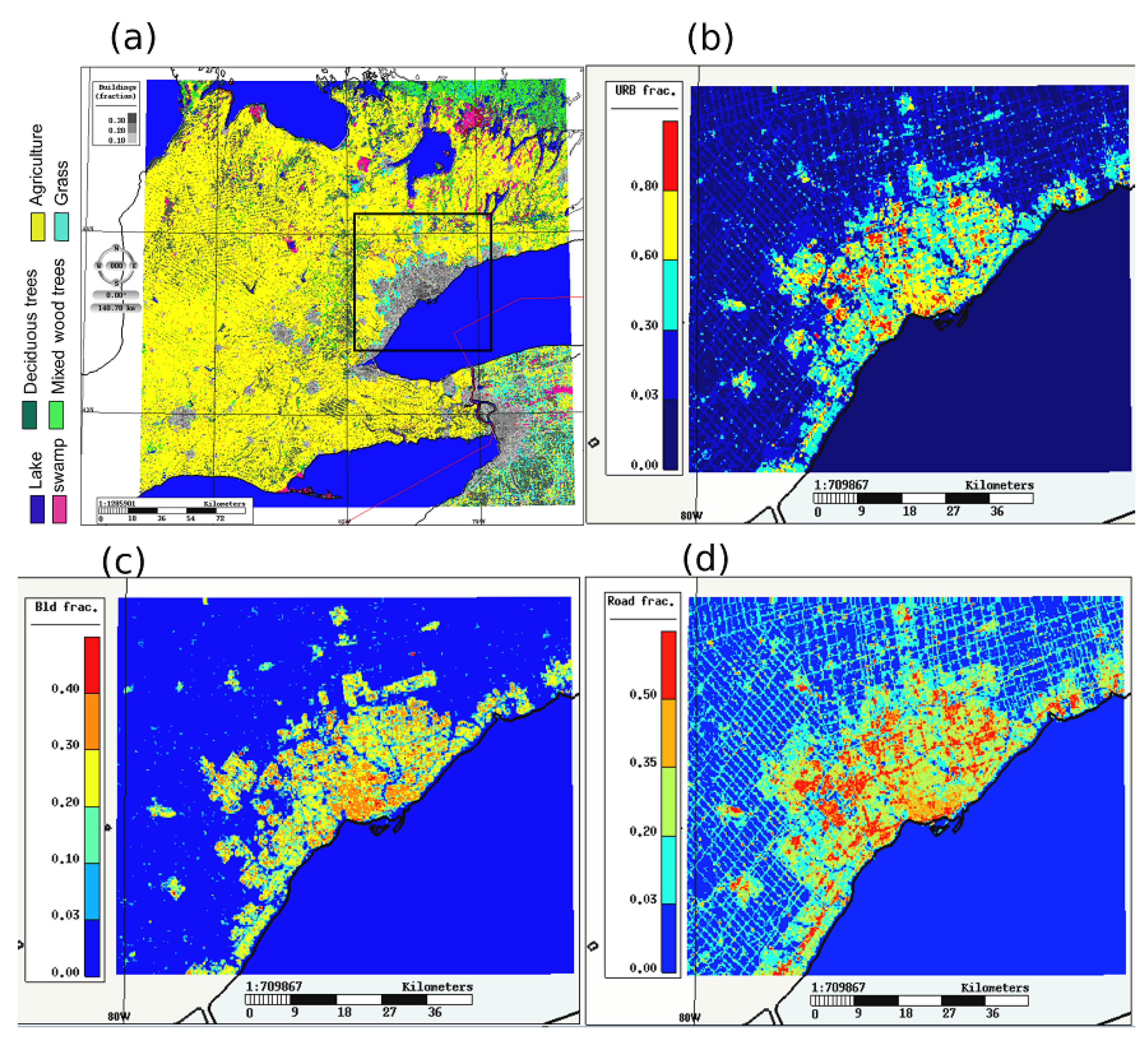
2.1.2. Surface Description

For domains with 250 m and 1 km grid spacing, orography was determined with the Canadian Digital Elevation Data (CDED-50) and the Shuttle Radar Topography Mission for the United States. Soil texture for the two soil layers used was determined from Agriculture and Agri-Food Canada (AAFC) and the United States Department of Agriculture. Particular attention was brought to TEB parameters and vegetation types at high-resolution. The former method used at ECCC [4], not available for Toronto, was updated by a more general method suitable for ECCC’s systems covering North America.

An overview of the production of high-resolution ancillary data and samples of the results over Downtown Toronto are provided in Figure 2. The method relies on the work of [49] who initially developed ECCC’s GIS tools to automate the production of refined Land Use/Land Cover (LULC) data in urban areas. Microscale (5 m) rasterized maps of detailed urban and natural classes (e.g., paved road, highway, unpaved road, residential area, commercial 24/7 building, city park, school, etc.) were produced by merging pan-Canadian databases (Figure 2a,b). The program was originally designed to facilitate the change or addition of databases. Further developments provided for this study are described hereafter. The national Topographic Data Base (NTDB) was replaced by the vectorial CanVec database provided by Natural Resources Canada to describe detailed LULC and occupancy over Canada. More vegetation attributes are described through the Land Cover Circa 2000 (LCC2000) detailed vectorial database. As the domain used in this study is covering two countries, for the United States the National Land Cover Database (NLCD) 2006 provides 30-m raster information of vegetation types, as well as vegetation and urbanization densities further downscaled at 5 m. In addition, the OpenStreetMap (OSM) database from 2013 is used to extract vectorial objects for roads and more precise land use descriptions where available. Then, the population density (2012 census data from Statistics Canada) has been updated and is used to sub-categorize residential areas. Moreover, detailed individual building heights provided by the City of Toronto for a region covering downtown Toronto with high-rise buildings were used to improve morphological description. Algorithms include a series of consistency verification and priority rules when needed based sometimes on subjective visual inspections.

Final TEB and ISBA input parameters were obtained by assigning 5-m values (following a look-up table, e.g., a 5-m pixel of parking corresponds to 100% of road in TEB, a city park with trees corresponds to the vegetation class of mixed forest), and then by aggregating results as illustrated in Figure 2c–e. Canopy parameters such as the mean building height, the canopy aerodynamic roughness length based on [50] parameterization, and the ratio of wall surfaces to horizontal area following [51] are computed directly on the model grid (Figure 2f,g). Final LULC for the inner grid is presented in Figure 3.

In addition to the presence of the city, the region has heterogeneous terrain and is surrounded by large lakes (including the Great Lakes) with complex water circulations. Therefore, integrated NWP relies on more advanced watershed representation.

2.1.3. Water Surface Temperature

Thermally-driven atmospheric circulations such as lake and land breezes are also likely to be better represented when the water surface heterogeneity is realistically specified. Sea and water surfaces temperature is initialized in HRDPS with a global analysis at 10-km resolution based on buoys measurements and remote sensing products [52] and remains constant through the day. The same method is used for TOR-GEM systems except for the Great Lakes basin which is the dominant watershed in the region. This study took advantage of the development of a coupled ocean-atmosphere system for the Great Lakes [53] that has since become the operational Water Cycle Prediction System [54] for both the Great Lakes (WCPS-GLS) and the Saint Lawrence River watersheds. It uses, respectively, the Nucleus for European Modelling of the Ocean (NEMO) model [55] for the physical processes in the water column and Community Ice CodE (CICE) for the evolution of ice properties above [56] and include river streamflow into the lakes. Lake surface temperature is provided at 2-km grid spacing every hour for the five Great Lakes. Values over the grids with 250-m and 1-km grid spacing were obtained by the use of WCPS specific interpolation-aggregation tools and a linear interpolation was made for time steps in between two values. It is worth mentioning that the system also assimilates in the same way ice extent and thickness throughout the winter.

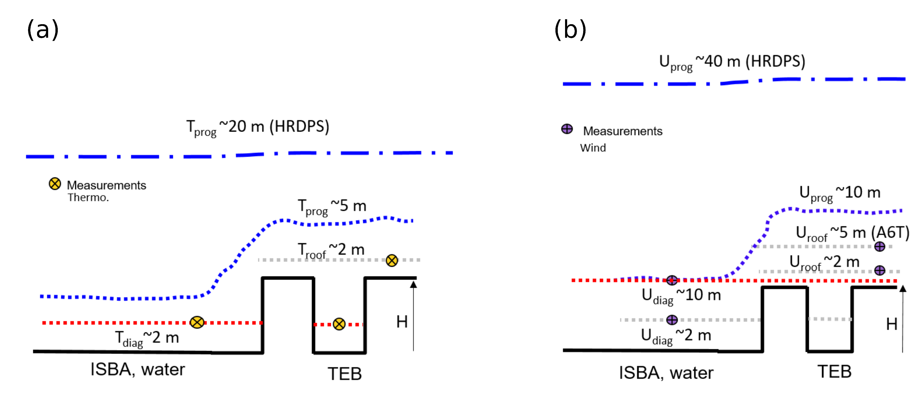
2.2. Comparison with Measurements

Data from both fixed and mobile measurements were used to evaluate the modelling system from 13 May and 31 August 2015 (corresponding to the period with the largest number of available measurements for PanAm) and their locations are mapped in Figure 4.

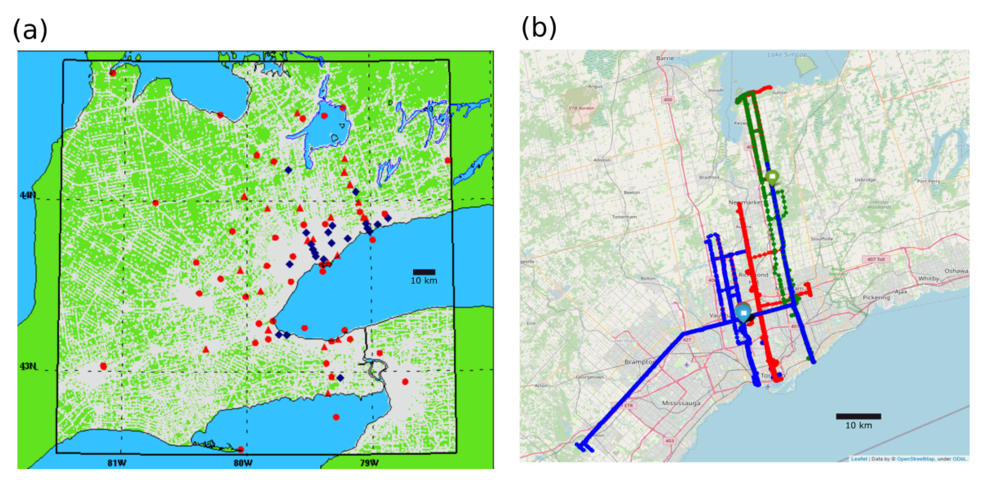
2.2.1. Surface Stations

First, most of fixed measurements sites are located in the region of Toronto, and near the Lake Ontario shoreline (Figure 4a). They are a combination of the operational ECCC surface station network that sparsely sample populated regions and the PanAm-specific stations that monitored GTA to a greater extent to capture urban features and track the inland propagation of the lake breeze [15,30]. Stations are classified into two categories, with 63 near-surface (including buoys) and 20 rooftop sites (details of stations are reported in Tables S1 and S2 of Supplementary Materials). Most of the instrumented buildings for rooftop stations were about 10 m tall and they were located in the urbanized regions of Toronto, Hamilton and Oshawa.

In order to evaluate model outputs near the surface, traditional diagnostic heights represented in the NWP systems are respectively about 2 m (10 m) above canopy level for the thermodynamic (wind) variables. A conceptual representation of the location of measurements and their corresponding modelled variables is presented in Figure 5.

Diagnostic wind at 10 m above ground level U${}_{diag}$ was computed directly in the TOR-GEM model depending on the canopy morphology. For grid points with buildings taller than 20 m, the wind speed is the street canyon wind speed [31]. For smaller buildings, the wind velocity value is either the atmospheric wind reduced by the logarithmic law, or a linear interpolation between the reduced wind and the canyon wind speed when 10-m height falls below the top of the canopy. For the ground stations, and due to unavailability of the canyon wind speed output data for the whole period of evaluation, only stations with wind measured at 10-m height are used in the objective evaluation.

Regarding the rooftop stations, velocities values U${}^{ref}$ at the first prognostic level ($z^{ref}$ = 40 m for HRDPS and z${}^{ref}$ = 10 m for TOR-GEM250) were corrected (during post-processing) to provide a fair comparison with the wind measured by the sensor U${}^{sensor}$ at z${}^{sensor}$ = 2.5 m above the roof (or at z${}^{sensor}$ = 5 m for one station as seen in Table S1 of the Supplementary Materials) using the following equation:

$$U^{sensor}=U^{ref}\frac{ln\frac{z^{sensor}+\frac{H}{3}}{z{0}_m}}{ln\frac{z^{ref}+\frac{H}{3}}{z{0}_m}},$$

(1)

with $z{0}_m$ the aerodynamic roughness and H the mean building height at the grid point (in m). Note that H is not defined in HRDPS. For temperature and dew point temperature, 5 m prognostic temperature in TOR-GEM250 is used for the full period comparison.

These features were implemented in the ECCC’s verification package presented in [20] to evaluate pan-Canadian short-range forecasts with the HRDPS. The tool performs several standard skill-scores and uncertainty is assessed with the bootstrapping method. In this study, Bias (BIAS) and standard deviation error (STDE) statistics are analysed for the prediction of near-surface temperature (T${}_{AIR}$), dew point temperature (T${}_D$), wind speed (U) and direction (U${}_{dir}$). Corresponding equations are reported in Appendix A.

Regarding precipitation forecasting skills, the Equitable Threat Score (ETS, [57]) is used to provide an overview of the model performance as detailed in Appendix A. It measures the forecasting performance of a system in its capacity to both represent an existing precipitation event and to avoid prediction of non-existing precipitation. Values fall between −1/3 and 1 and the closer that ETS is to 1, the better the precipitation forecast.

2.2.2. Mobile Measurements

The second database is the ECCC Automated Mobile Meteorological Observation System (AMMOS, [15]) which provides near-surface meteorological data for 21 days (mostly daytime) during the summer of 2015 for three instrumented cars. Routes were large arterial roads but not highways, sampling the central part of GTA (Figure 4b, and see Section S1 of Supplementary Materials). They were following three parallel routes from the shoreline and the downtown to about 19 km north, sometimes up to 35 km at King City (at the location of ECCC’s radar), and more rarely, up to Lake Simcoe. A few itineraries were covering the area parallel to the Lake Ontario shore (at about 19 km away). Data used in this study are from quality-controlled meteorological data averaged at 1-min interval (original measurements were at 1-s interval). Temperature and dew-point temperature from AMMOS are compared with model values at the nearest grid points. Given the fact that there were four times fewer quality-controlled measurements for wind than for temperature and that more analyses would need to be performed, wind data are not retained in this study. In addition to bias and STDE, the linear correlation coefficient r is computed for the scatter plots evaluation of these data (Appendix A).

3. Results and Discussion

3.1. High-Resolution Weather Prediction

A selection of results demonstrating the capacity of TOR-GEM250 to represent more realistic meteorological patterns is presented in this section. Due to the numerous outputs and physical processes to be considered with this system, the reader is invited to consult other specific companion studies where model outputs from this system were used. For example, Ref. [30] have evaluated thermal stress indices newly implemented in the system. Ref. [58] have analyzed the modeled lake-breeze system for two cases with light and strong inland penetration with both Lidar and surface measurements.Prediction of lightning occurrences has been evaluated at different resolutions [59].

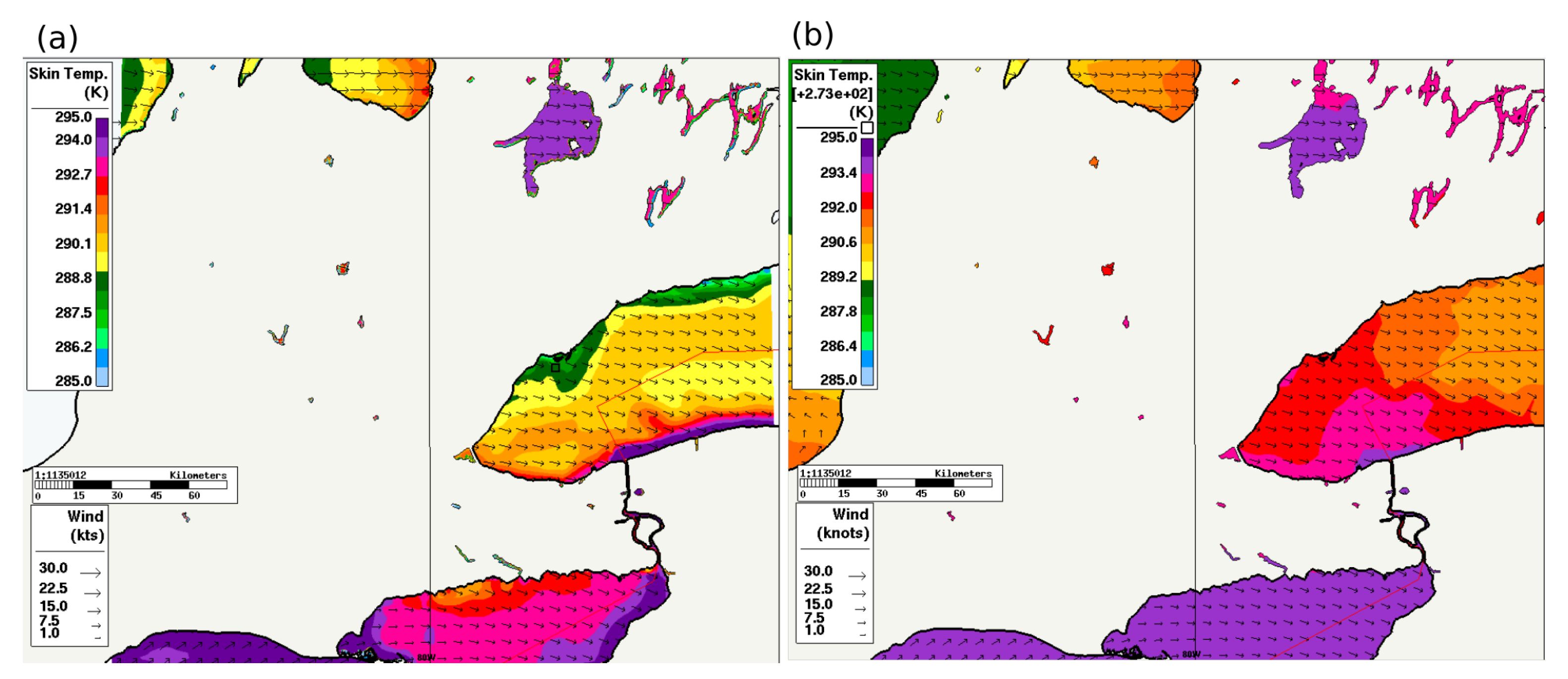
3.1.1. Coastal Upwelling

The impact of the integration of improved lake surface temperature on the NWP system is investigated here. In particular, the northern Lake Ontario shore is subject to frequent upwelling resulting in cooler near-shore water temperature values in summer [60], and water flows between Lakes Erie and Ontario at different background temperatures. Figure 6a shows a map of water skin surface temperature on the grid with 250-m grid spacing on a day with offshore north-west synoptic wind (23 July 2015), which exhibits colder temperatures near the shore as a signature of an upwelling process in the watershed. Buoy measurement close to the Toronto islands is in agreement with the assimilated temperature. An important gradient of 9 °C can be observed between the north and the south shores of Lake Ontario for this event as the opposite downwelling process occurs on the southern shore. Lake Erie is warmer but still exhibits lower temperatures on the north shore. As can be seen in Figure 6b, the operational global analysis of water surface temperature (Figure 6b, see Section 2.1.3) exhibits less spatial variability over Lake Ontario and does not consider colder temperatures on the north shore. Similar differences can be seen for Lake Erie. This analysis is, however, used to prescribe daily Lake Simcoe (located in Figure 1c) and other water bodies surface temperatures. The hourly assimilation of the lake water temperature then allows for a more detailed representation of gradients occurring in the region.

3.1.2. Urban-Scale Heterogeneity

Urban-scale summertime 2015 general features are presented in this section. Averaged 15-min results were computed for canopy-top turbulent fluxes and near-surface meteorological variables for the period between 13 May and 31 August 2015. Time evolution of the different variables reflects the energy budget partitioning in and out urban areas [4,33].

Detailed results over the GTA are presented in Figure 7 at 2000 EDT corresponding to 18 h after initialization. At this time of the day slightly before sunset, spatial distribution of values of turbulent fluxes, surface temperature at different heights and dew point temperature varies. Figure 7d exhibits larger and positive sensible heat flux values over the GTA with values up to 60–70 W m${}^{-2}$ in the downtown region with high-rise buildings near the shore. More energy is released into the atmosphere after being stored during the day in the tall canopy where radiation fluxes were trapped previously. Over natural surfaces, sensible heat flux returns to a slightly negative value which is an expected behavior at that time [4]. Map of the latent heat flux (Figure 7e) shows values below 40 W m${}^{-2}$ in GTA as compared to values in the surroundings reaching 100 W m${}^{-2}$ over agricultural land outside the GTA, with minimum values in downtown and around the metropolitan area ring, where more impervious surfaces are present (such as industrial and commercial areas and large highways, as seen in Figure 3d). Over Lake Ontario, sensible and latent heat fluxes have small absolute values due to small vertical gradient of temperature and humidity at that time.

Skin radiative surface temperature (Figure 7a) exhibits a clear distinction of urban areas similarly to the sensible heat flux. Values reach 25 °C downtown but no more than 13 °C above Lake Ontario. These large temperature gradients through the warm season contribute to the enhancement of lake breezes processes in the region.

As felt by standing persons at about 2-m above ground level, air temperature intra-urban variability has clearly a different spatial distribution (Figure 7b) than the skin surface temperature. Larger values are still found in correlation with highly urbanized pixels, but the maxima are found over a region slightly north of the downtown and extends into surrounding urban areas due to advective air movements. In particular, maximum temperature values are seen in an industrial region with few vegetation and more absorbing materials at the south-west of the highways intersection (see Figure 3d, and identified in Figure S4 of the Supplementary Materials by the business improvement area in the city yard 7). A stable air layer is found over Lake Ontario with an air temperature minimum value of 15 °C, 2 °C larger than surface temperature. In between the lake and the GTA, a sharp temperature gradient is found near the shore. It is likely that colder air from the lake, and the air layer over the densely built areas warmed earlier in the daytime, were advected to the North by the often occurring lake-breeze flow.

As a result of more complex mesoscale circulations through the day, less spatial correlation between the urban area and the warmer air temperature is seen at the first prognostic atmospheric level at 5-m above the canopy level (Figure 7c). A region with diluted contours with larger temperature remains over the urban areas and illustrates the regular presence of a canopy urban heat island (CUHI) over Toronto. One can note, however, that the maximum values are also reached in the vicinity of the two green valleys respectively along the Don (East side of downtown) and Humber (west side of downtown) rivers (Figure 1c). A wider region than in Figure 7b of colder air is found near the shore, as cool air from the lake is advected aloft an internal urban boundary-layer.

Dew point temperature (Figure 7f) at the first atmospheric level exhibits the lowest values over the central areas of Toronto and north of it, even lower than over the lake. On the contrary to the lowest values, the largest dew point values are correlated with regions of the largest latent heat fluxes over the vegetation north and west of Toronto.

Daily time series for the corresponding domain and period are represented in Figure 8. Values are averaged based on the LULC clusters following Figure 3b urban fraction (URBF) thresholds. As seen in Figure 8a, near-surface air temperature reaches maximum values of 23.5 °C around 1500 and 1600 EDT for the most urbanized grid points. The effect of using initialization based on a lower-scale model is seen as air temperature is relatively homogeneous during the 7–8 h after the initialization over land. Later and until the end of simulations, values decrease as the urban fraction decreases. Regarding the quantitative description of the daytime CUHI, it is respectively 8 °C (2.5 °C) between the densest area of the city and the watershed (and the rural grid points). Early in the night, air temperature above the lake and in the surroundings of the city (with URBF < 30%, see Figure 3b) becomes similar but the regions forming the core of the city remains warmer, by about 1.8 °C. Standard deviation values among clusters are small, about 0.2–0.3 °C but are slightly larger for the densest cluster (URBF > 80%). This might be due to the effect of other urban descriptors or to the effect of the distance to the lake.

Figure 8b exhibits similar trends for the radiative surface temperature values with average maximum values of 34 °C. Diurnal variations are however much larger (up to 20 °C as compared to about 9.5 °C except for the lake water. The largest heterogeneity among clusters is seen for densest areas and for the lake water with the standard deviation reaching 3 °C. During daytime, resulting skin–air surface temperature difference presented in Figure 8c remains negative over water and increases progressively with the urban fraction categories with large positive values up to 10 °C. All clusters identify the air layer to return to a nighttime stable state but with a time lag of 4 h from the rural regions to the densest grid points. This is in agreement with the sensible heat flux evolution in the evening with remaining positive values until respectively 1900 LST (2300 LST) for the rural (most urbanized) category (Figure 8e). Sensible heat flux also exhibits the maximum 2 h later for the most urbanized pixels than for the rural grid points, with about double values (260 W m${}^{-2}$ and 120 W m${}^{-2}$). Heat trapped into the urban canopy during daytime is then released to the atmosphere in the evening and in the early night through sensible heat in addition to surface radiative cooling. By contrast, the latent heat flux becomes homogeneous through the urban regions at 2100 EDT (Figure 8d). Daytime values are maximum over rural regions (350 W m${}^{-2}$), with large difference among clusters.

The Bowen ratio (sensible to latent heat flux ratio) in Figure 8f highlights the evolution of the partitioning of the thermodynamic turbulent fluxes. During daytime when both fluxes are positive above land, it varies from a plateau not exceeding 0.5 for the fewer urbanized pixels (less than 30%) but reaching 1 and above for denser grid points. The more the urban fraction, the less regular is the curve. It is obvious for pixels with URBF > 80%, where two maximum values of about 3.5 are reached at 1230 EDT and 1800 EDT. In between, values slightly smaller highlight the time for the maximum of the latent heat flux at about 1530 EDT whereas maximum for the sensible heat flux occurs earlier at 1400 EDT.

Impact of lake-breeze flows on GTA’s intra-urban CUHI is further investigated in the following paragraph. During the Games period (from 8 July to 15 August), 95% of the days featured lake-breeze development [15]. Figure 9 presents maps averaged for days with low deformation lake-breeze over the lake Ontario (10, 11, 27, 28 July and 15 August 2015). Low deformation lake breeze means that the influence of the synoptic-scale wind is low and that the lake breeze propagates inland parallel to the coastline [61]. Maps of air temperature are provided during daytime (1500 EDT) and night-time (0100 EDT). During daytime (Figure 9a), air temperature maximum values are found over the city but at about 10 km north of the shoreline. During nighttime (Figure 9b), maxima are found close to the shore and concentrated around Toronto downtown, due to the interaction of the land breeze with the persistent heat released in urban areas (release of energy stored during the day). These results are in agreement with the expected climatology for coastal city under lake-(or sea-) breeze regime (see Figure 2 in [1]). In those situations, the maximum CUHI over land reaches respectively 5 °C (7 °C) for daytime (nighttime), but with a strong anisotropy for daytime with almost 14 °C as compared to the water side.

As shown in this section, the system is able to capture the heterogeneity of the surface-atmosphere interactions due to detailed representation of the urban, rural and water surfaces at very high resolution. The amplitude of the CUHI varies through the time of the day and the level of urbanization, but also to the meteorological conditions and the proximity to water bodies. Comparison with previous studies is therefore exploratory. For example, Ref. [62] found a CUHI of 0.7 °C (2 °C) respectively for daytime (night-time) for Toronto during a heat-wave with the Weather Research and Forecasting (WRF) model. However, intensities were based on a few grid points with locations that were not especially representative of the maximum/minimum in the region and the urban fabric heterogeneity for Toronto and its surrounding remained unrefined even with 333-m grid spacing. For Chicago which is another coastal urban agglomeration under the influence of the Great Lakes, and with the same model with 1-km grid spacing, similar nocturnal CUHI values of about 2 were found in [63]. Maximum temperature values during daytime were also found away from the coast, at about 15–30 km, with results sensitive to the description of the urban canopy. GTA’s summertime meteorology is influenced by the lake-breeze flow. Characteristics of such mesoscale circulations are further analyzed in the following section.

3.1.3. Mesoscale Meteorology

The TOR-GEM250 grid covers the region of Southern Ontario between Lakes Ontario, Erie, St. Clair, Huron (including Georgian Bay), and Simcoe (starting south of GTA and going clockwise) which has been intensively studied for its frequent occurrence of thermally-induced pressure gradients at the shores responsible for mesoscale circulations such as lake-breeze (and land-breeze) often responsible for convective patterns [61,64,65] and air chemistry features [64].

An illustration of the development of multiple lake-breeze fronts in the study region on 18 July 2014 is shown in Figure 10. Due to weak synoptic flow on that day, low-deformation lake-breeze circulations developed allowing the lake breeze to penetrate well inland around each lake, as seen on a visible satellite imagery at 1450 EDT from the MODIS Aqua radiometer (Figure 10a). Cumulus cloud development over the region in between the lake-breeze fronts can be identified with the spatial organization of significant surface-based convection, with more intense convection to the south. At 10 min apart, Figure 10b shows an analysis of the lake-breeze fronts as retrieved with the iCAST nowcasting system and using both GOES satellite, radar observations and in-situ measurements. These two products provide coherent information on the location of the fronts, including the merger of two fronts in one thin frontal zone in the Niagara peninsula (between Lakes Ontario and Erie). It should be noted that the location of lake breeze fronts is not identical to the visible cloud edges.

Forecasting of this situation is shown at the same time as the satellite with grid spacing of 250 m (Figure 10c,d). Predicted cloud cover exhibits the same organization as the visible satellite image. Multiple lake breezes with inland propagation can be identified with a South-East wind blowing over the GTA (Lake Ontario), a westerly wind blowing over the West of the domain (Lake Huron) and a southerly wind blowing over Lake Erie’s north shore. In agreement with MODIS, a region with less clouds along the southern Lake Huron’s coast can be seen (with the cloud edge forming a curve). This region corresponds to convective rolls in the region with moderate wind (due to the lake-breeze flow) upwind of the formation of inland cellular convective cells (as seen in Figure S2 in Supplementary Materials). Enhanced cloud development over the Oak Ridges Moraines can be seen as well, although slightly more than in MODIS. Clouds forming at the edge of Lake Erie’s front are slightly larger than in the north in both MODIS and TOR-GEM250. As was observed that day, the onset of the lake breeze occurred earlier on that shore (1200 EDT), allowing sufficient time for the convection to intensify.

Predicted surface winds with manually identified lake-breeze fronts annotated are presented in Figure 10d. Such evaluation of subkilometer-scale weather predictions can be difficult in a highly turbulent atmosphere and has some degrees of uncertainties [58,66]. While the synoptic wind was weak that day, indicators such as horizontal wind velocity, wind confluence, as well as associated updrafts and downdrafts, were found to be the most relevant (see Figures S2 and S3 in Supplementary Materials). Results of TOR-GEM250 suggest that lake-breeze fronts between Erie and Ontario did not fully merge, but the frontal zone is more clearly defined for the Lake Ontario shore (Figure S5c). The mesoscale analysis suggests that lake-breeze fronts have merged (Figure 10d), but this was not yet the case one hour before which suggests that the situation was evolving fast. Front collision in the Niagara peninsula is regularly occurring as described for two case studies with 200-m grid spacing simulations with WRF and mesoscale analysis [66]. Interestingly, as the grid spacing is increasing in the predictions for the nesting grids up to 10 km, cumulus clouds are also found in the same region but they are less numerous and tend to be larger, and the representation of the frontal zone becomes less detailed (Figure S4 in Supplementary Materials). TOR-GEM250 provides the best comparison with the satellite image. It is worth mentioning that the clouds in the satellite image are even smaller in some areas, which suggests that the model with 250-m grid spacing still does not have sufficient resolution to fully represent their organizations. Characteristics of the modelled lake-breeze front, more likely the turbulent structures than the location, might be impacted by the current one-dimensional planetary boundary-layer scheme used, as shown recently in [25] for idealized simulations using several turbulent schemes.

In summary, despite the complexity of the local scale atmospheric daytime evolution in summer, this section has highlighted the capacity of the TOR-GEM250 model to reproduce the impact of the lake-breeze currents propagation on the convective organization in the region. These mesoscale features are important in this region in summertime and can be associated with diverse effects, such as cooling of the coastal urban regions, air pollutant transport, or the occurrence of convective precipitation. Preliminary analysis of the precipitation patterns are examined hereafter.

With seasonal averaging (from 13 May to 31 August 2015) similar to that in the previous Section 3.1.2, Figure 11 shows afternoon and evening 6 h accumulated precipitation amounts between 1400 and 2000 EDT (Figure 11a), and between 2000 and 0200 EDT (Figure 11b). In the afternoon (Figure 11a), larger values are found generally inland, at some distance from the lakes coasts. Maxima are found in the south-west region and in the centre of the land areas, with largest values in the region of the city of London, ON. Lower values are found over Toronto and north of it, with slightly more accumulation around the Oak Ridges Moraine outcrop north of Toronto. Minimum is found over the middle of the Great Lakes. These patterns can be explained by the prevalence of lake breezes inland and air mass advection towards slightly more elevated regions (Figure 3c).

In the evening and later (Figure 11b), the accumulation of precipitation exhibits different spatial patterns. Large values are still found on the west part. A west–east oriented band with large values can be seen from Burlington to a region near Kitchener and the south of the small Conestogo Lake. It is possible that this pattern corresponds to the area where the lake breezes from different lakes sometimes interact and the convergence intensification is likely to produce more precipitation, but it also likely corresponds to advection of leftover convection from storms during the day. Over the Great Lakes, larger values were found than earlier in the day, likely due to end of the lake breeze flow and possibly the onset of land breeze flow. The Toronto area did not receive much precipitation that season as compared to the rest of the domain, as the lake breeze is often occurring and propagates beyond the agglomeration borders, and as latent heat flux is smaller over the GTA. To assess the realism of these maps, results were compared with Canadian Precipitation Analysis (CaPA) available for that period with 10-km grid spacing [67]. Unfortunately, the scale resolved by the background field is too coarse to provide a meaningful evaluation of TOR-GEM250 precipitation. Evaluation at surface stations will be therefore performed in the next section.

This section has provided an analysis of the capacity of the TOR-GEM250 system to provide detailed and realistic representation of the meteorology in and around a city for the GTA area. Further evaluation with in-situ measurements is provided in the following section.

3.2. Objective Evaluation

In this section, following the methodology in Section 2.2, evaluations are provided over the inner modelling domain with 250-m grid spacing (Figure 1) with both the surface monitoring network and the mobile meteorological measurements, and TOR-GEM250 is compared with the reference ECCC’s HRDPS system for short-range forecasting in Canada.

Time series evaluations are presented for the 24 h of the simulation for TOR-GEM250 and for the operational HRDPS system initialized at the same time, for both surface and rooftop stations. Corresponding local time starts at 0200 EDT.

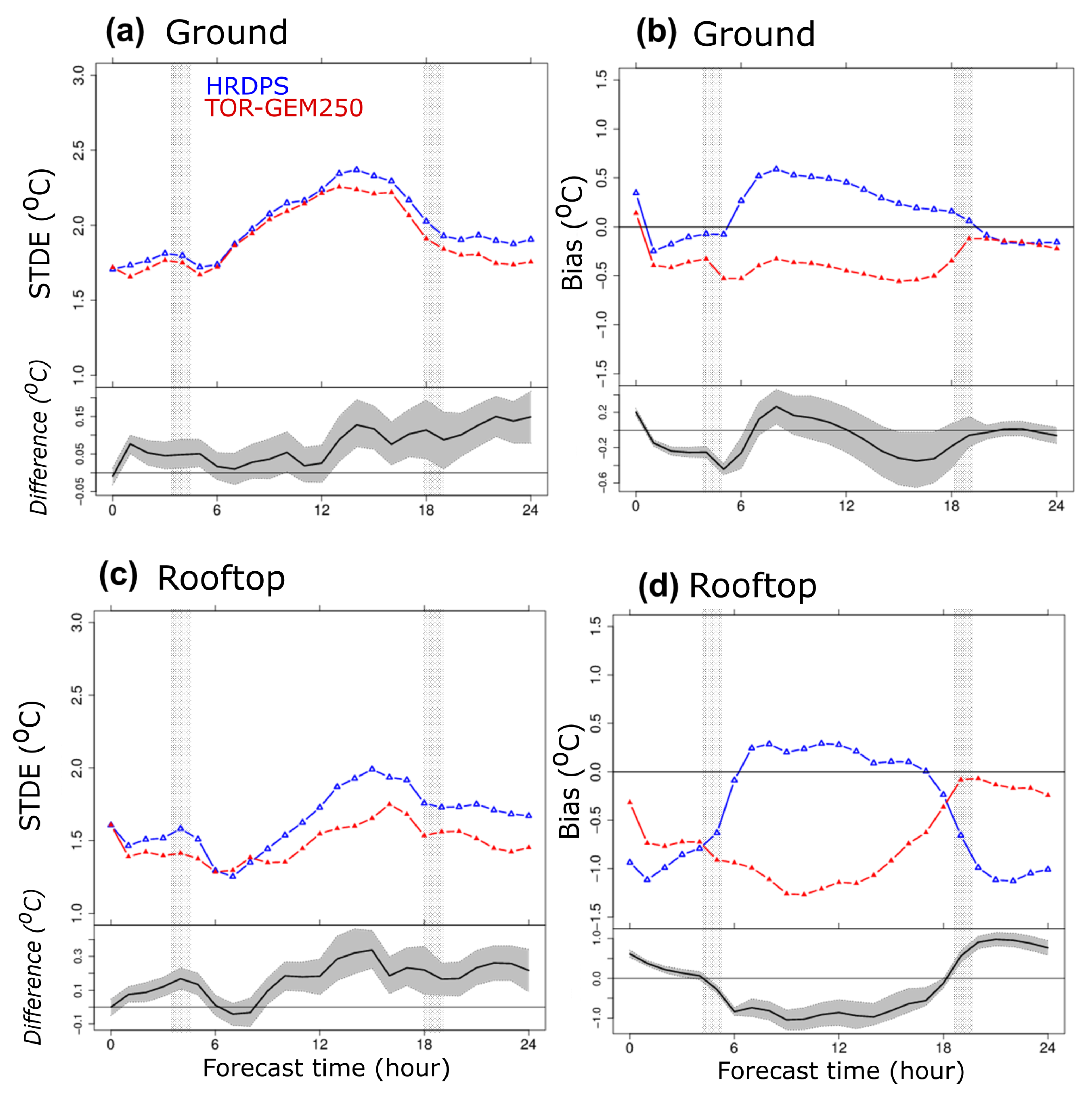
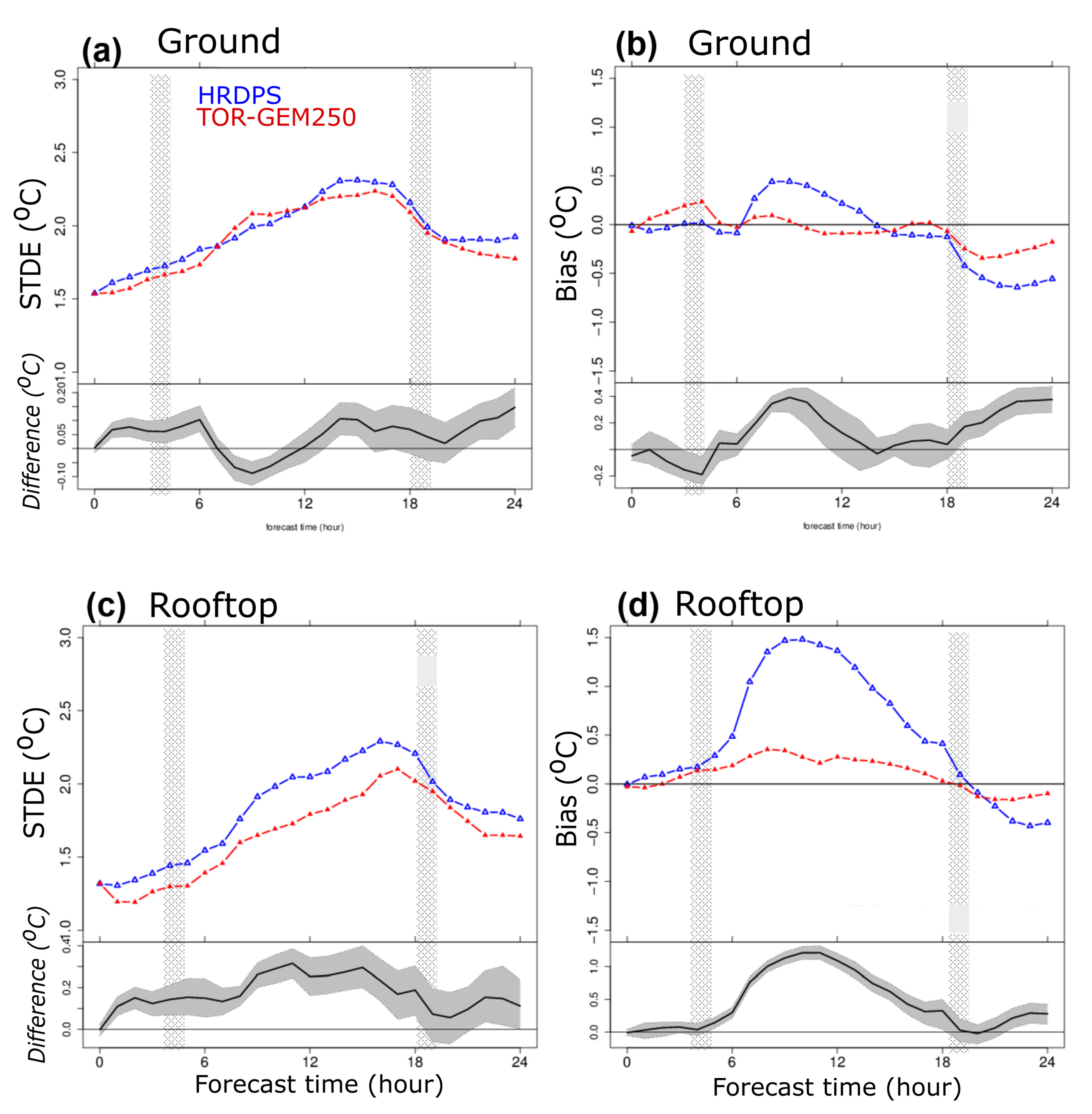
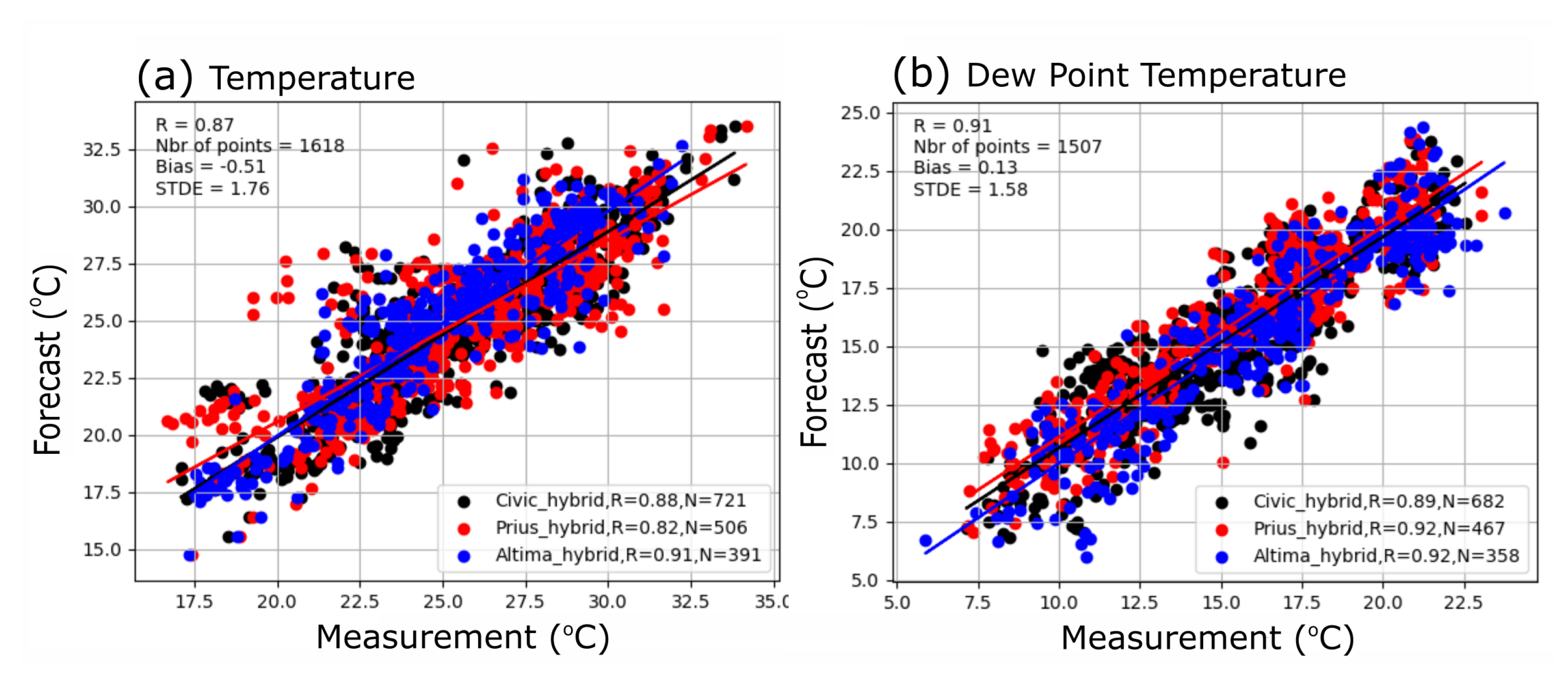
3.2.1. Temperature and Dew Point Temperature

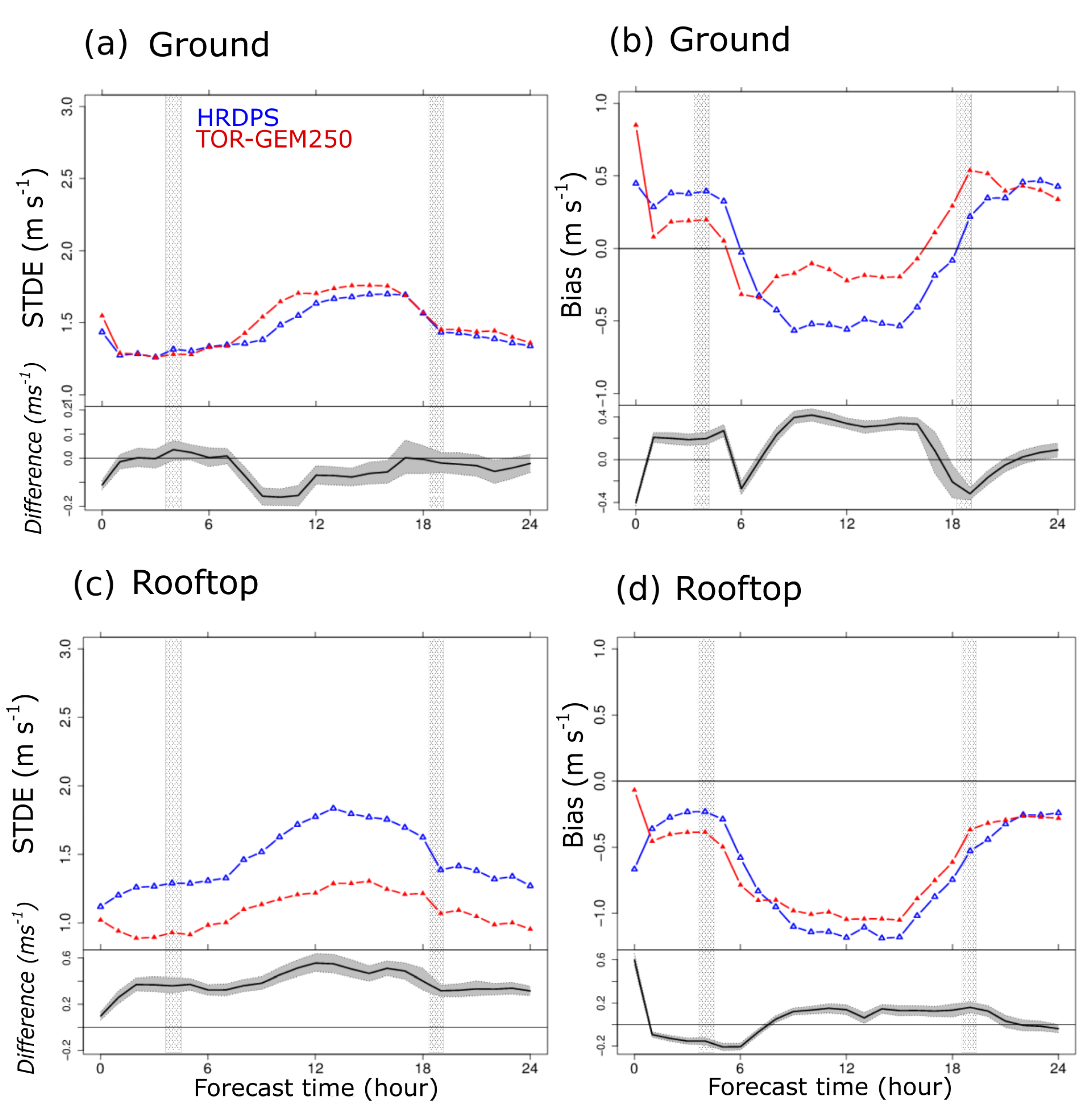
Statistics for temperature are shown in Figure 12. For surface stations, STDE values for 2.5-m above ground level $T_{2.5m}$ are consistently lower for TOR-GEM250 than in HRDPS (Figure 12a). Improvement is small but existing for the first 12 h. It is likely that the simplified initialization of TEB’s prognostic variables limits the performance of TOR-GEM250. STDE improvement increases however with time and reaches 0.15 °C by the end of the simulation, highlighting the better representation of spatial variability in temperature. Diurnal cycle of the errors is similar between the two experiments, with larger errors during daytime. Corresponding bias (Figure 12b) shows a slight underestimation of air temperature through the day for TOR-GEM250 of less than 0.5 °C and decreases for the second night to about 0.15 °C. In comparison, bias in HRDPS is either negative during the night with the same value than TOR-GEM250 after sunset and it features a positive maximum of 0.6 °C occurring after sunrise. Ground stations are located in mixed environments with significant vegetation fractions. Therefore, the role of evapotranspiration processes after sunrise in ISBA plays an important role in air temperature warming and might be overestimated in HRDPS.

With overall similar trends for the rooftop stations, statistical improvement of TOR-GEM250 over HRDPS is even larger than for ground stations, up to 0.3 °C in the STDE (Figure 12c) in late afternoon. There is less amplitude in the error diurnal cycle for TOR-GEM250, in particular for hours following sunrise, probably due to the impact of a better representation of physical processes over built-up surfaces. Bias is improved during nighttime (less negative). During daytime HRDPS shows substantial temperature overestimation (up to 0.2 °C). TOR-GEM250 exhibits an underestimation in a larger extent (up to 1.3 °C). As was mentioned earlier, the modeled variable from HRDPS and TOR-GEM250 above the roof are slightly different (see Section 2.2.1). As buildings are represented in TOR-GEM250 the variable compared with measurements is featured at 5-m above roof level.

The impact of such a difference between the temperature at the first prognostic level (T${}_{5m}^{prog}$) and a temperature diagnosed directly above the roofs at the sensor level (T${}_{2.5m}^{diag}$) is shown in Figure 13 on averaged for 5 days when the variable was stored from the system for further investigations. Unstable conditions are found with (T${}_2$${}^{diag}$) up to 1.35 °C warmer than (T${}_5$${}^{prog}$) for the maxima, which is likely to explain the daytime negative bias in Figure 12d. Although this is shown for a few days only, it is argued that it might have an impact for the four and a half months period.

Air water vapor content is traditionally evaluated in NWP with the dew point temperature, as it impacts numerous surface and boundary-layer processes. On Figure 14 is shown STDE and bias of T${}_D$ at 2.5-m above ground level and 5-m above roof level. Near the ground (Figure 14a), STDE are lower in TOR-GEM250 than in HRDPS during the first 6 h of the simulations, slightly larger during the next 6 h, and lower again until the end of the simulation by 0.15 °C. This result indicates that the spatial variability is better represented in the new system. Bias is relatively small (Figure 14b) for the two systems between −0.6 and 0.5 °C, but it is even smaller after 6 h of simulation in TOR-GEM250, almost nonexistent until the sunset after which the bias is improved by up to 0.4 °C in comparison to HRDPS. The bias has fewer diurnal variations as the fraction of impervious area in the surrounding of the station is better represented. The difference of representation of the buildings and roads between the two systems is obvious over the rooftop stations (Figure 14c,d). STDE errors remain improved during all the simulation and up to 0.3 °C during the afternoon, which is statistically significant. Due to the overestimation of the evapotranspiration of the soil and vegetation in HRDPS the bias for rooftop station is large and reaches 1.4 °C in the morning. In TOR-GEM250 the bias is improved by 1.3 °C during daytime and still by 0.4 °C during the second night. The diurnal cycle is less present in TOR-GEM250 as the fraction of vegetation is likely to be better represented.

To complement the objective evaluation, comparison of model outputs with mobile measurements is performed and provides sampling of different areas than the fixed mesonet. They covered the denser regions of the city from the downtown to city suburban rings (Section 2.2.2). Predicted versus measured scatter plots for all measurements are shown in Figure 15 for the mobile stations. Good correlations are found for the temperature (Figure 15a) and dew point temperature (Figure 15b) with relatively similar statistics for the three cars. The bias (STDE) for temperature is −0.52 °C (1.76 °C) which is rather consistent with results in Figure 12; and for the dew point temperature, respectively 0.13 °C (1.58 °C), which demonstrates a better STDE than for Figure 14. Good linear correlation coefficient is found for air temperature (0.88) and dew-point temperature (0.91).

This section has demonstrated the good performance of TOR-GEM250 for temperature and dew point temperature forecasting during the summer of 2015 for various locations. Heterogeneity in suburban areas is also improved as compared with HRDPS in particular for the second part of the runs. The wind speed is the next variable to be evaluated.

3.2.2. Wind Field

Wind vectors exhibit more details when forecasted at high resolution. The representation of built-up surfaces also tends to reduce the mesoscale wind [7]. These changes are highly dependant on the location of the measurement sites. This section is however exploring if objective evaluation can be informative on the new system performance.

As seen in Figure 16a for the ground stations, STDE errors are relatively similar for the two systems and are comprised between 1.3 m s${}^{-1}$ during nighttime and 1.75 m s${}^{-1}$ during daytime. The error increases earlier in TOR-GEM250 and remains above the one in HRDPS between 8 to 16 h of simulation (10 to 18 EDT). This time corresponds however to an improved bias as seen in Figure 16b with increased wind speed by up to 0.4 m s${}^{-1}$. Bias tends to remain smaller in TOR-GEM250 during the night, and slightly larger at sunset, despite a similar STDE than HRDPS. Differences in these figures might be due to the larger spatial variability of the wind field resolved in TOR-GEM250 and in particular due to the detailed representation of the urban canopy.

For the rooftop stations, STDE errors for TOR-GEM250 are significantly improved as compared with HRDPS during all the time series by up to 0.5 m s${}^{-1}$ in the middle of the day and of about 0.3–0.4 m s${}^{-1}$ during the nights (Figure 16c). Values are relatively similar in HRDPS for ground and rooftop stations. By contrast, values drop to 0.9–1 m s${}^{-1}$ during the night for TOR-GEM250, and 1.25 m s${}^{-1}$ during the day. This result indicates that TOR-GEM250 provides a better performance in the forecasting of the wind field heterogeneity in the coastal urbanized areas where rooftop stations are located. Corresponding bias values in Figure 16d suggest however a wind speed underestimation in both systems, by 1.2 m s${}^{-1}$ in HRDPS and 1 m s${}^{-1}$ in TOR-GEM250 in the middle of the day and respectively by 0.25 m s${}^{-1}$ to 0.4 m s${}^{-1}$ during the night. It is possible that the method used to adapt the forecasted wind field to the roof level decelerates the wind too much. It is worth mentioning that a revision of Equation (1) taking into account the static stability was tested for several cases resulting in relatively few differences. Evaluation of the wind direction was relatively similar between the two systems (Figure S5 of the Supplementary Materials).

Overall, results suggest objectively that the wind speed is generally improved in TOR-GEM250 for rooftop stations with a remarkable improvement of the STDE all day in comparison to HRDPS. STDE is increased for the ground stations in particular during daytime. It is possible that the very large wind heterogeneity in TOR-GEM250 in the complex summertime situations with cellular convection organization augment the statistical errors found at point stations. Summertime simulation with WRF with 333-m grid spacing over Toronto also revealed more difficulties to compare the wind with surface measurements than the temperature [62].

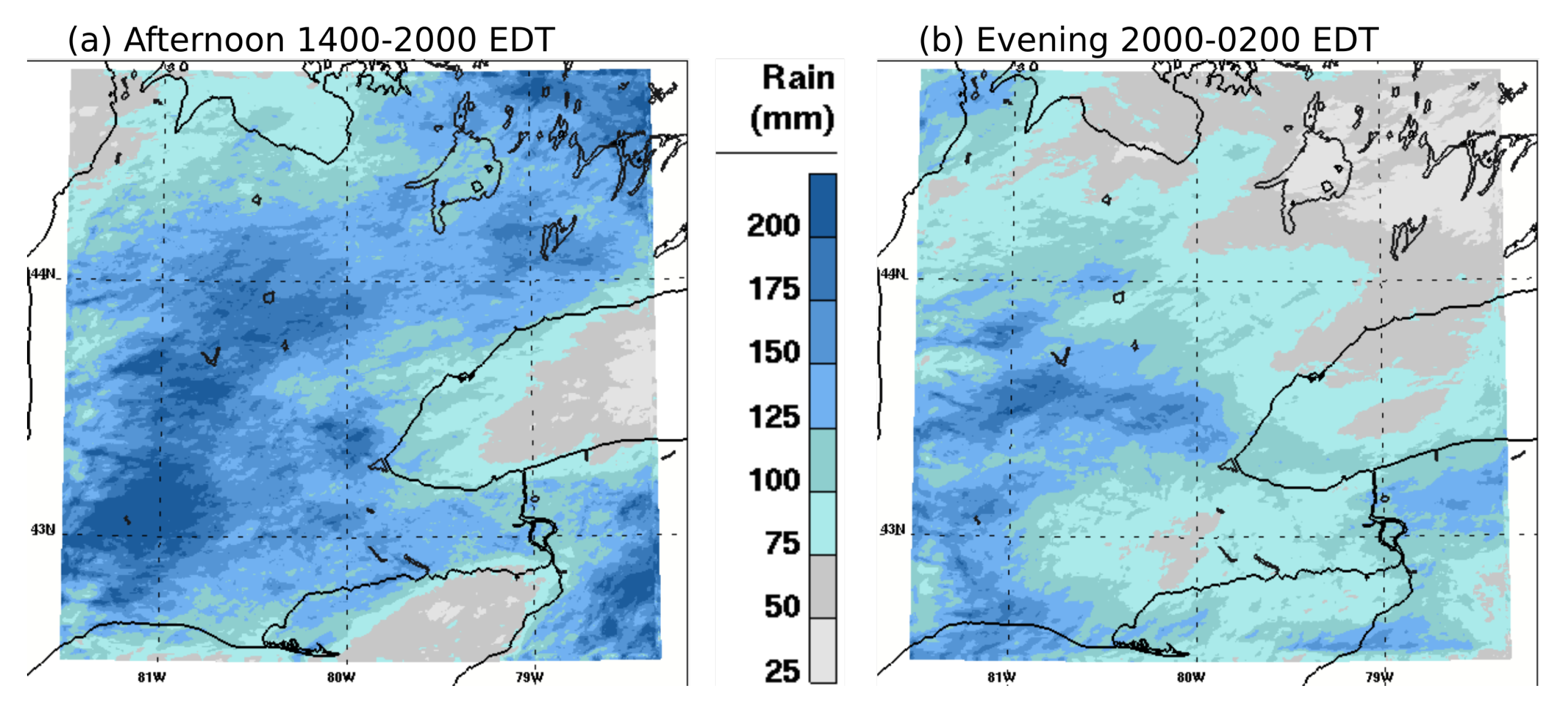
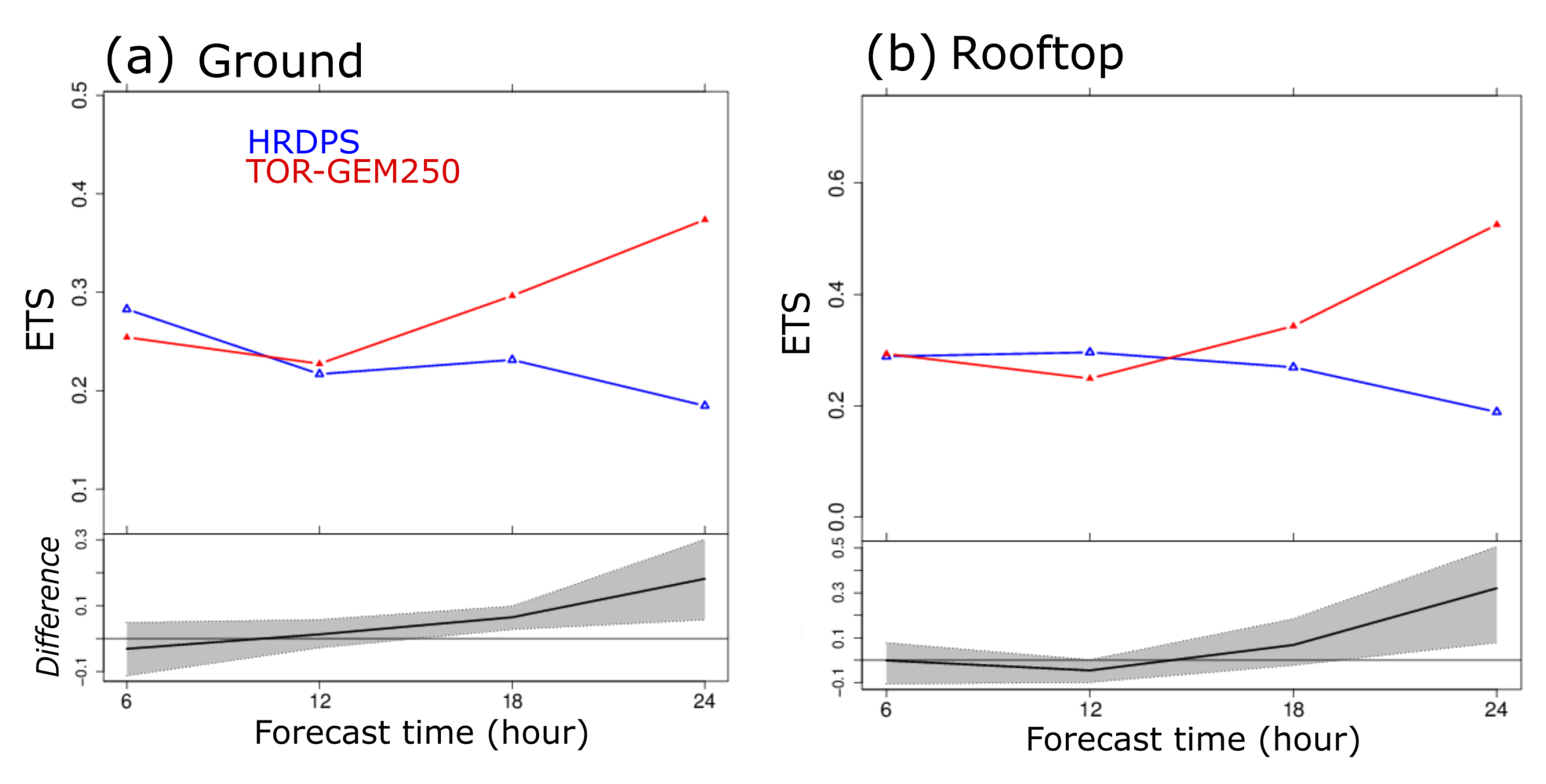
3.2.3. Precipitation

The spatial distribution of surface stations reported in Figure 4 is relatively dense in the centre of the domain, in and around the Toronto Greater area and along the lake Ontario’s coast. There are unfortunately less stations available in the western agricultural landscape that would help evaluating precipitation patterns in Figure 11. ETS (Section 2.2.1) is presented for results exceeding an accumulation of 5 mm during 6 h for the forecasting lead times 6, 12, 18 and 24 h, for the ground (Figure 17a) and rooftop (Figure 17b) stations. During the first part of the simulation (6 and 12 lead time), TOR-GEM250 exhibits a similar score than HRDPS or slightly below (between 0.22 and 0.29 for ground stations and between 0.25 and 0.3 for the rooftop stations). Later, ETS is significantly improved in TOR-GEM250. ETS is respectively improved for ground (rooftop) stations from 0.23 (0.23) in HRDPS to 0.3 (0.35) in TOR-GEM250 for precipitation accumulation between 12 and 18 h lead time and from 0.18 (0.19) in HRDPS to 0.38 (0.55) in TOR-GEM250 for precipitation accumulation between 18 and 24 h lead time.

The results indicate that TOR-GEM250 clearly outperforms HRDPS in precipitation forecasting after 12 h of simulations. This increase of performance with time indicates that TOR-GEM250 requires sufficient spin-up period or it needs improved initial conditions. Other results considering various precipitation amount thresholds confirm the good performance of the system for the second part of the simulations, with the exception of an overestimation of events with very small amount (see Figure S6 in Supplementary Material), which could be due to measurement uncertainties. The results also underline that TOR-GEM250 is more capable of representing the summertime convective precipitation occurring in late afternoon and evening.

4. Summary and Conclusions

Real-time NWP at high-resolution for urban areas and their surroundings is an important step towards the delivery of multiple services to city stakeholders, with model outputs directly available, or as a component of comprehensive decision-making tools. This paper presents results from the experimental TOR-GEM250 system set-up over the GTA and run in real-time in the context of the PanAm Games in Toronto prior to and during the summer of 2015. A detailed procedure to obtain geographical surface descriptors to be used by the surface schemes was followed. This method is now further used in all-scale NWP and air-quality systems with TEB at ECCC (currently up to 2.5 km). Forecasts were produced at grid-spacing as low as 250 m with optimized configuration. Their quality has been demonstrated both objectively, with results at surface stations and mobile measurements, and subjectively with analysis of small-scale meteorological patterns. The main results and perspectives are summarized as follows:

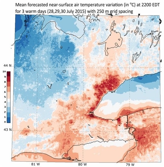
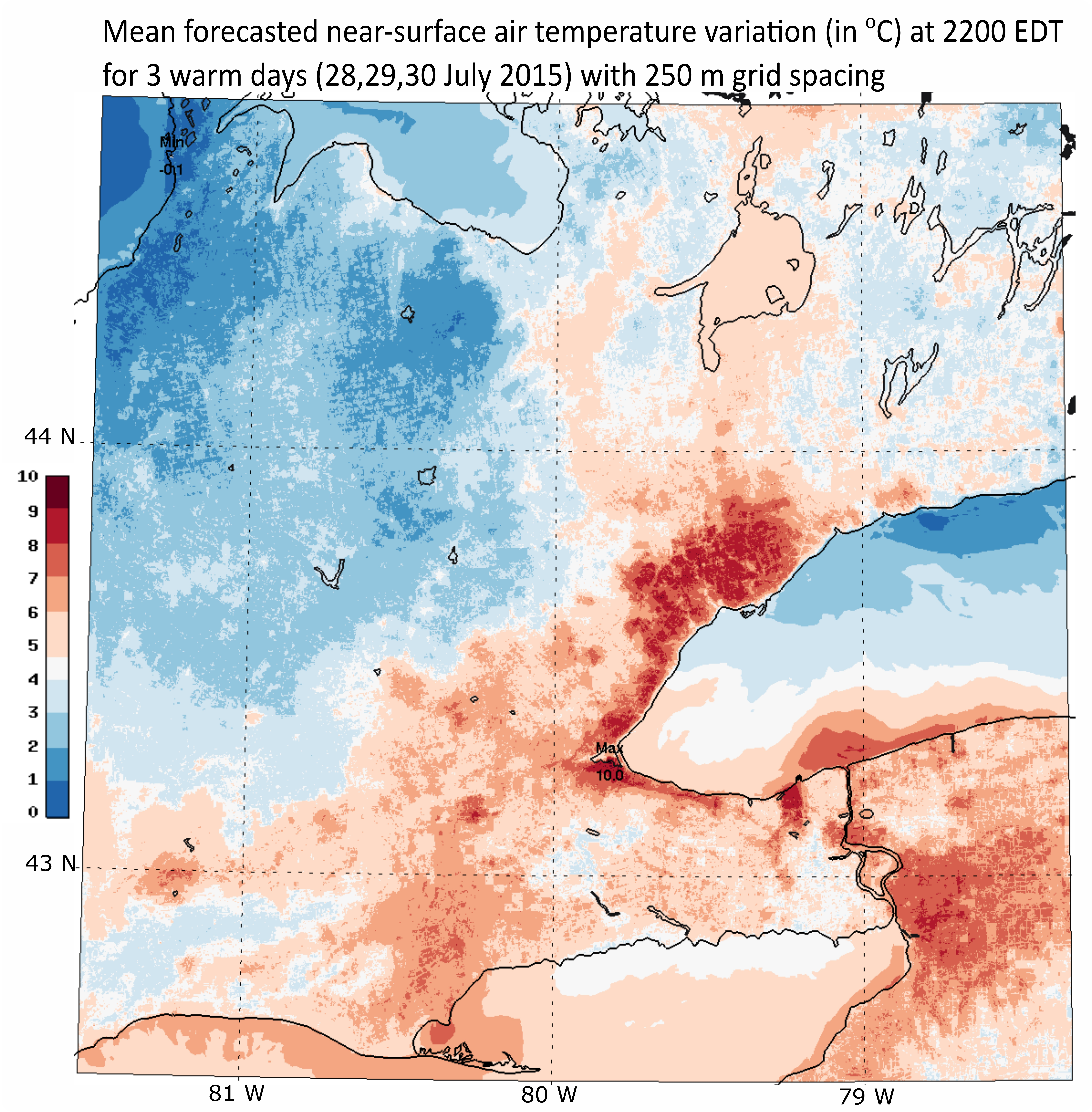
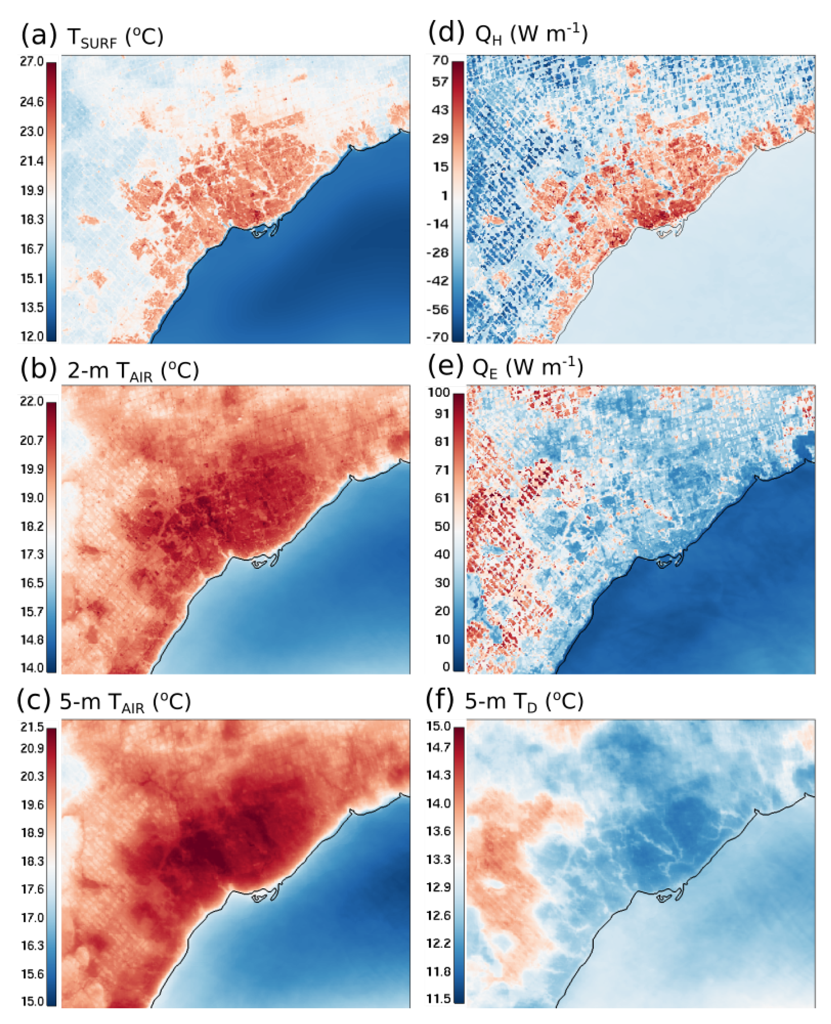
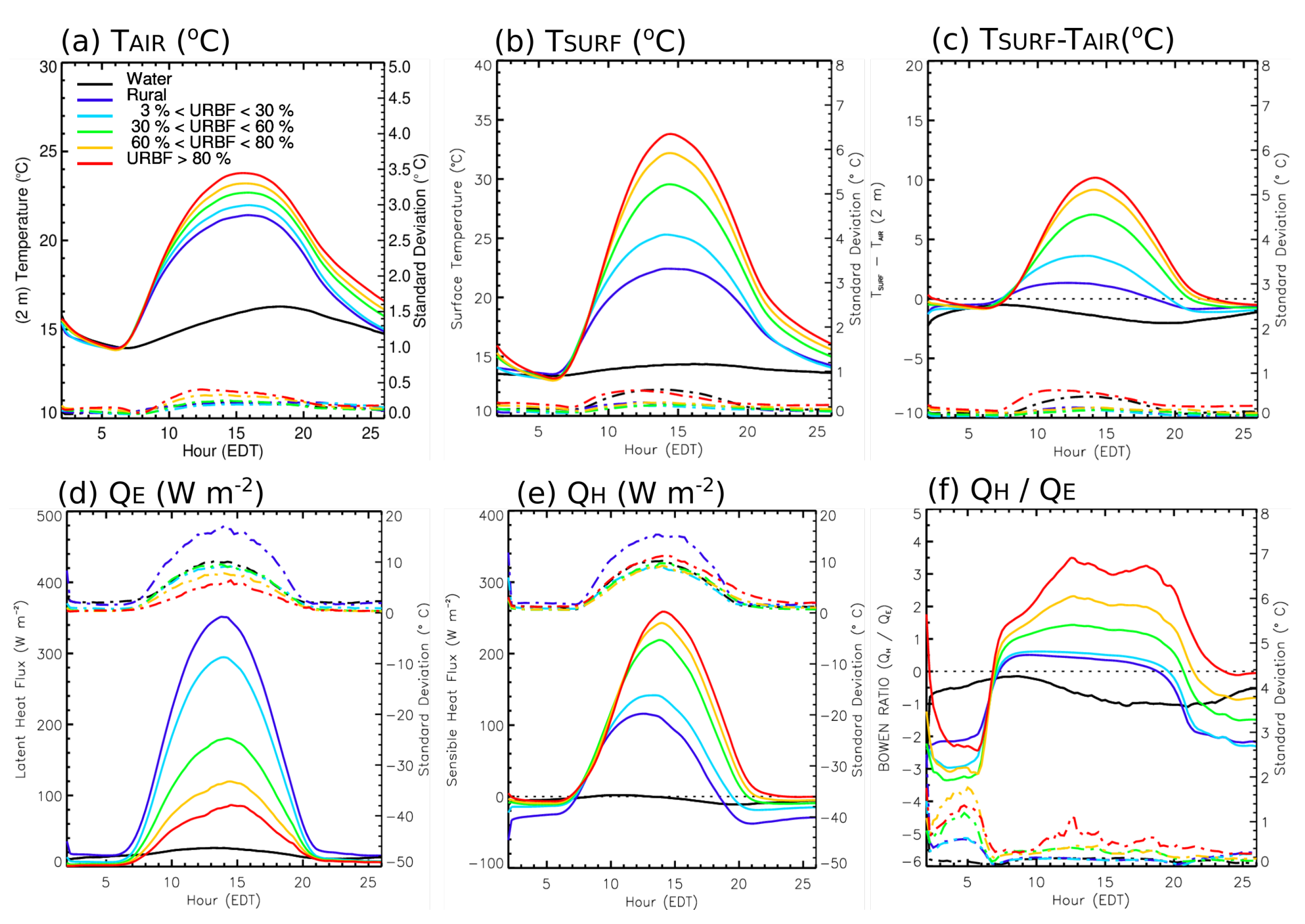
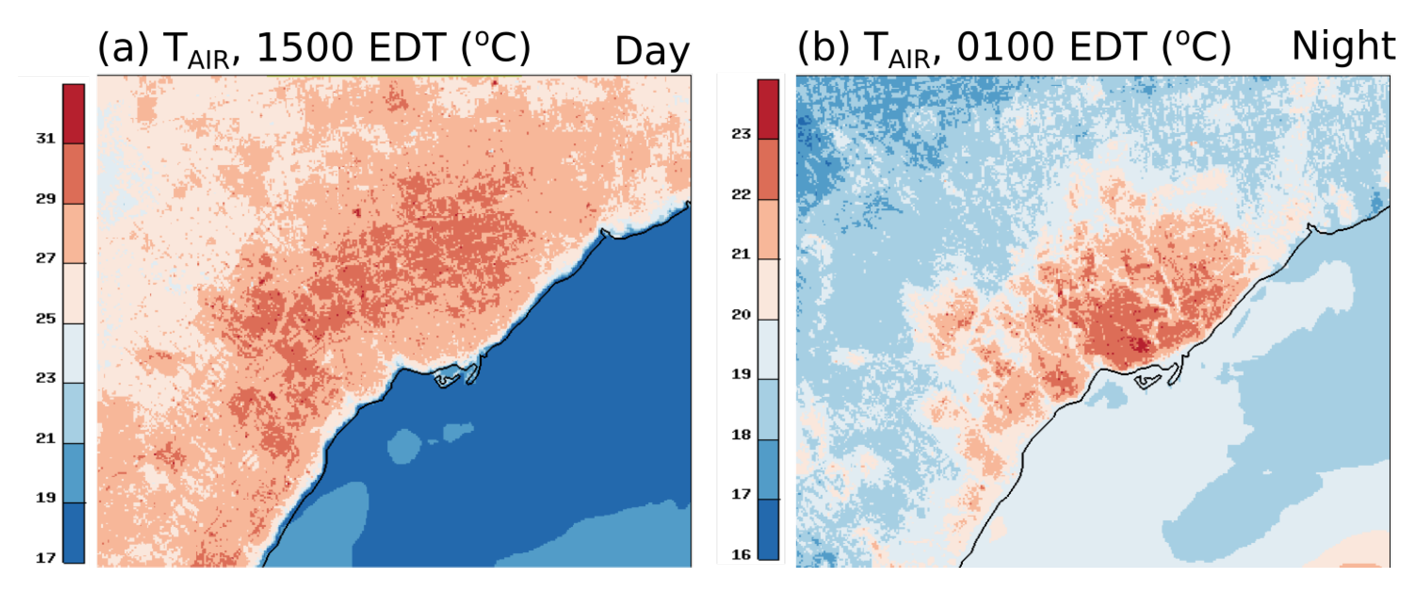
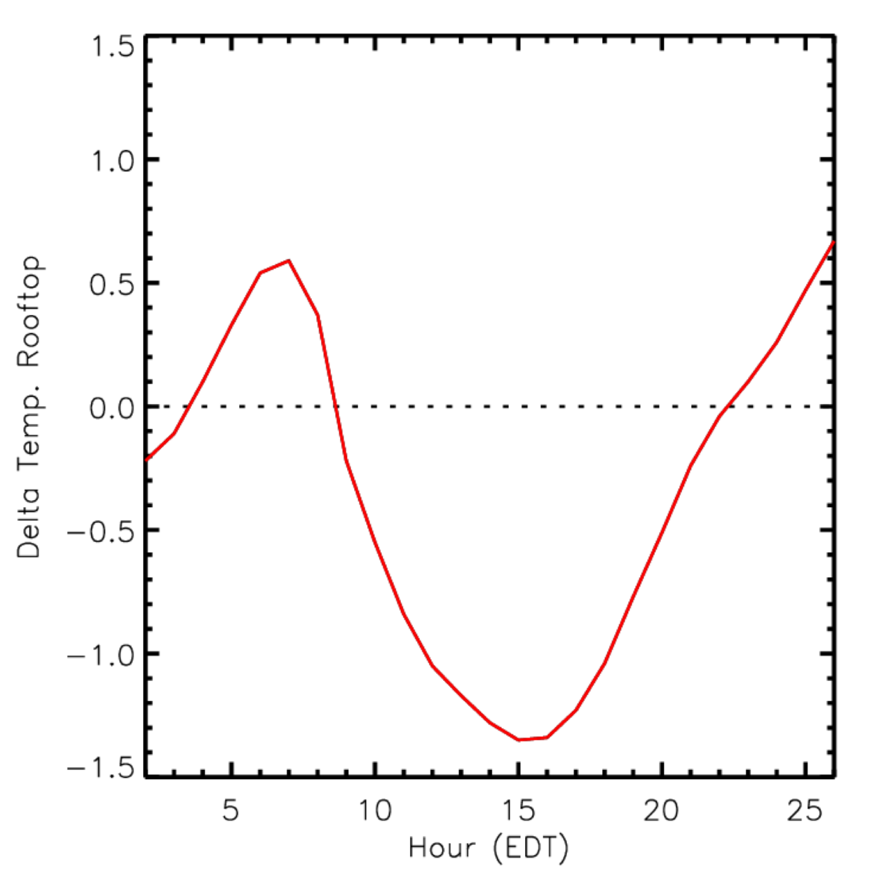
• The intra-urban scale micro-meteorology is predicted thanks to the representation of the urban fabric heterogeneity. Analysis of thermodynamic patterns over the summer season provides information on the characteristics of the GTA UHI which is important for both day, with a strong anisotropy, and night. On average for the season, CUHI is about 2 °C considering the rural surroundings. In details, it is about 1.8 °C during the night and 2.5 °C during the day as compared to the northern side of the city, and up to 8 °C during the day on the Lake Ontario side of the city. Contrasts can even reach 14 °C for some days in July when a low-deformation lake breeze penetrates inland. Urban-water surface contrasts are particularly large for this region which increase the impact of the city in the surface differential heating responsible for air advection and convergence zones. In the evening, heat stored in the urban canopy is restituted to the atmosphere through sensible heat flux in addition to surface radiative cooling;
• A further step towards an integrated system is reached in this study with the prescription of time-evolving Great-Lakes surface temperature based on realistic physical processes in the watershed. This additional factor in the representation of small-scale heterogeneity is influencing atmospheric circulations. Further development could include inline coupling of atmosphere and ocean processes at the same high-resolution (as is the case at ECCC for the global scale), or assimilation of in-situ buoys temperature. It is worth mentioning that surface temperature evolution over the Great Lakes have been successfully evaluated at a larger spatio-temporal scale [53], but more evaluation at the microscale would be needed as well. In particular there still can exists situation with some bias could be responsible for a lack of representation of the lake breeze system with potential impacts on the simulation of air pollutant dispersion in the GTA [9];
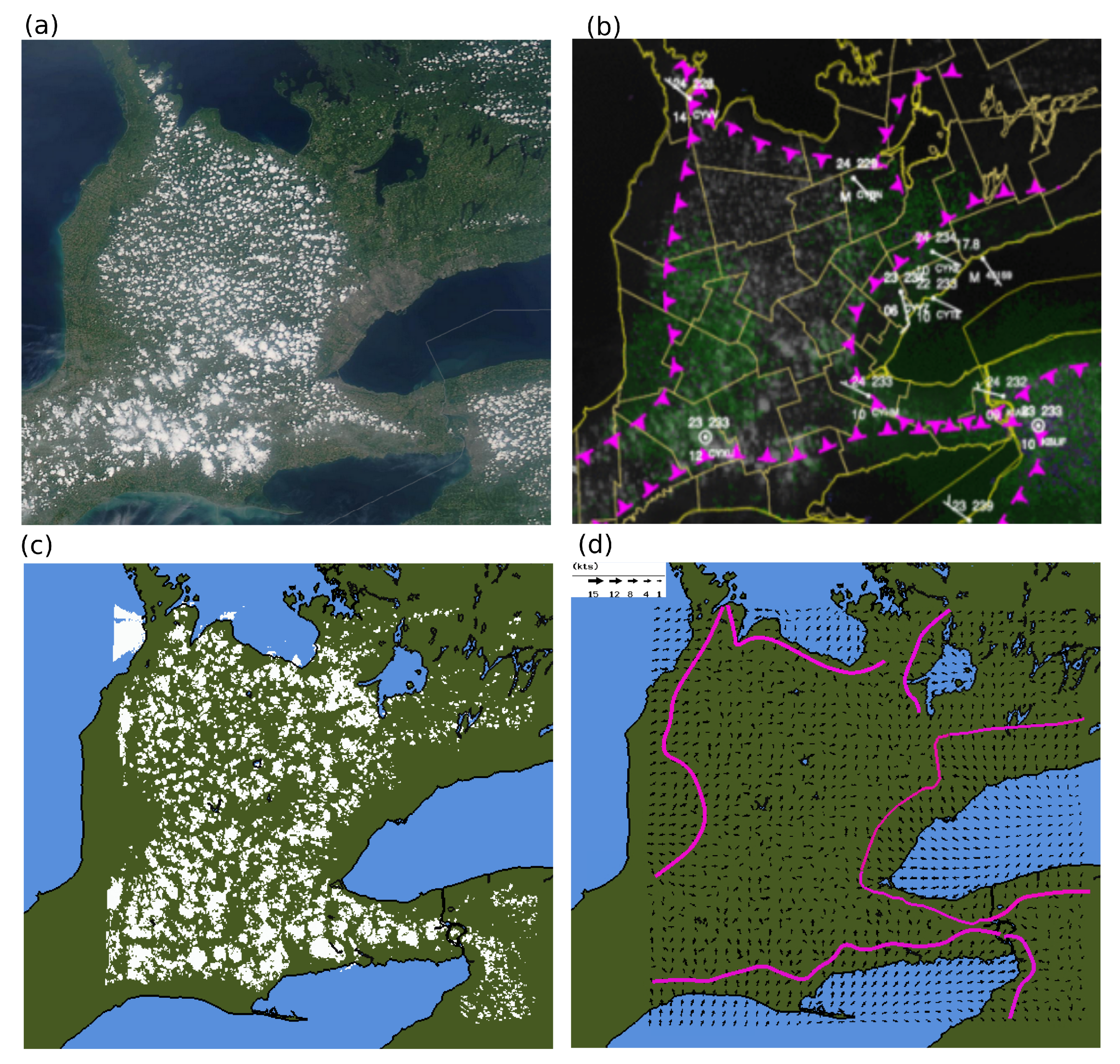
• Lake-breeze systems are important patterns in the GTA region and impact the local meteorology. Subjective comparison of TOR-GEM250 cloud patterns with satellite imagery on a day with lake breezes on multiple Great Lakes highlights the capacity of the system to provide realistic meteorological results which are not achieved by lower resolution systems. A complete objective analysis of lake breezes for the whole summertime season would be of interest;
• The real-time experimental system, TOR-GEM250, outperformed MSC’s HRDPS for all variables and in particular for the second part of the simulation, as evidenced by objective evaluation with 83 in-situ surface stations and mobile measurements. The system improves particularly the standard deviation errors through the day, which indicate that such a system would be valuable to represent small-scale variability in and around the city. This improvement reaches 0.3 °C for temperature and dew-point temperature and 0.5 m s${}^{-1}$ for wind speed. A method to evaluate model output with measurements located both at the ground and at rooftop level has been suggested in this study. The authors advise to carefully consider the sensor height to evaluate the model output with the variable that is intended to represent the measured value. Additional evaluation of the wind field’s intra-urban variability will also be required. Further investigation would be needed to assess the representativeness of the wind measured very close to surface (at about 2 m) as is the case for the AMMOS mobile stations and for some of the fixed stations.
  It also appears that the system is not optimal in the first few hours of the simulation. In the near-future, emphasis on the more accurate initialization of TEB prognostic variables and soil moisture in urban areas will be deployed. Method currently under investigation include the recycling of variables, and/or the implementation of the urban areas in the CaLDAS assimilation system [68];
• Precipitation patterns include many more details in TOR-GEM250 than in lower resolution systems and in particular for the late afternoon and evening events. Improvement of objective evaluation at stations with ETS reaching 0.55 for the evening period in urban areas indicates that the refined system better represents the meteorology. The city of Toronto and its surroundings do not receive a lot of precipitation as compared to the rest of the domain. This kind of system could be used to develop a very high-resolution precipitation analysis that would provide important information for many sectors of activities. For example, recent development of an ECCC’s 2.5 km ensemble-based precipitation analysis system still fail to fully represent summertime convective precipitation [69];
  Finally, the ongoing replacement of the microphysics scheme and, more generally, the modernization of the physics in GEM [70] for ECCC’s NWP systems is also likely to improve the forecasting of clouds and precipitation properties. Enhancement in several aspects of the predictions can be expected with an adaptation of the turbulent subgrid scheme to the grey zone of turbulence [24,71].

References

1. Masson, V.; Lemonsu, A.; Hidalgo, J.; Voogt, J. Urban Climates and Climate Change. Annu. Rev. Environ. Resour. 2020, 45, 411–444. [Google Scholar] [CrossRef]
2. Grimmond, S.; Bouchet, V.; Molina, L.T.; Baklanov, A.; Tan, J.; Schlünzen, K.H.; Mills, G.; Golding, B.; Masson, V.; Ren, C.; et al. Integrated urban hydrometeorological, climate and environmental services: Concept, methodology and key messages. Urban Clim. 2020, 33, 100623. [Google Scholar] [CrossRef] [PubMed]
3. Baklanov, A.; Cárdenas, B.; Cheung Lee, T.; Leroyer, S.; Masson, V.; Molina, L.T.; Müller, T.; Ren, C.; Vogel, F.R.; Voogt, J.A. Integrated urban services: Experience from four cities on different continents. Urban Clim. 2020, 32, 100610. [Google Scholar] [CrossRef] [PubMed]
4. Leroyer, S.; Bélair, S.; Mailhot, J.; Strachan, I.B. Microscale Numerical Prediction over Montreal with the Canadian External Urban Modeling System. J. Appl. Meteorol. Climatol. 2011, 50, 2410–2428. [Google Scholar] [CrossRef]
5. Ronda, R.J.; Steeneveld, G.J.; Heusinkveld, B.G.; Attema, J.J.; Holtslag, A.A.M. Urban Finescale Forecasting Reveals Weather Conditions with Unprecedented Detail. Bull. Am. Meteorol. Soc. 2017, 98, 2675–2688. [Google Scholar] [CrossRef]
6. Li, H.; Zhou, Y.; Wang, X.; Zhou, X.; Zhang, H.; Sodoudi, S. Quantifying urban heat island intensity and its physical mechanism using WRF/UCM. Sci. Total Environ. 2019, 650, 3110–3119. [Google Scholar] [CrossRef] [PubMed]
7. Leroyer, S.; Bélair, S.; Husain, S.Z.; Mailhot, J. Subkilometer Numerical Weather Prediction in an Urban Coastal Area: A Case Study over the Vancouver Metropolitan Area. J. Appl. Meteorol. Climatol. 2014, 53, 1433–1453. [Google Scholar] [CrossRef]
8. Bélair, S.; Leroyer, S.; Seino, N.; Spacek, L.; Souvanlasy, V.; Paquin-Ricard, D. Role and Impact of the Urban Environment in a Numerical Forecast of an Intense Summertime Precipitation Event over Tokyo. J. Meteorol. Soc. Jpn. Ser. II 2018, 96A, 77–94. [Google Scholar] [CrossRef] [Green Version]
9. Stroud, C.A.; Ren, S.; Zhang, J.; Moran, M.D.; Akingunola, A.; Makar, P.A.; Munoz-Alpizar, R.; Leroyer, S.; Bélair, S.; Sills, D.; et al. Chemical analysis of surface-level ozone exceedances during the 2015 Pan American Games. Atmosphere 2020, 11, 572. [Google Scholar] [CrossRef]
10. Mailhot, J.; Bélair, S.; Charron, M.; Doyle, C.; Joe, P.; Abrahamowicz, M.; Bernier, N.B.; Denis, B.; Erfani, A.; Frenette, R.; et al. Environment Canada’s Experimental Numerical Weather Prediction Systems for the Vancouver 2010 Winter Olympic and Paralympic Games. Bull. Am. Meteorol. Soc. 2010, 91, 1073–1086. [Google Scholar] [CrossRef] [Green Version]
11. Bernier, N.B.; Bélair, S.; Bilodeau, B.; Tong, L. Near-Surface and Land Surface Forecast System of the Vancouver 2010 Winter Olympic and Paralympic Games. J. Hydrometeorol. 2011, 12, 508–530. [Google Scholar] [CrossRef]
12. Joe, P.; Doyle, C.; Wallace, A.; Cober, S.G.; Scott, B.; Isaac, G.A.; Smith, T.; Mailhot, J.; Snyder, B.; Belair, S.; et al. Weather services, science advances, and the Vancouver 2010 Olympic and Paralympic Winter Games. Bull. Am. Meteorol. Soc. 2010, 91, 31–36. [Google Scholar] [CrossRef] [Green Version]
13. Kiktev, D.; Joe, P.; Isaac, G.A.; Montani, A.; Frogner, I.L.; Nurmi, P.; Bica, B.; Milbrandt, J.; Tsyrulnikov, M.; Astakhova, E.; et al. FROST-2014: The Sochi winter Olympics international project. Bull. Am. Meteorol. Soc. 2017, 98, 1908–1929. [Google Scholar] [CrossRef]
14. Golding, B.; Ballard, S.; Mylne, K.; Roberts, N.; Saulter, A.; Wilson, C.; Agnew, P.; Davis, L.; Trice, J.; Jones, C.; et al. Forecasting capabilities for the London 2012 Olympics. Bull. Am. Meteorol. Soc. 2014, 95, 883–896. [Google Scholar] [CrossRef]
15. Joe, P.; Belair, S.; Bernier, N.; Bouchet, V.; Brook, J.; Brunet, D.; Burrows, W.; Charland, J.P.; Dehghan, A.; Driedger, N.; et al. The environment Canada pan and parapan American science showcase project. Bull. Am. Meteorol. Soc. 2018, 99, 921–953. [Google Scholar] [CrossRef]
16. Hidalgo, J.; Masson, V.; Gimeno, L. Scaling the Daytime Urban Heat Island and Urban-Breeze Circulation. J. Appl. Meteorol. Climatol. 2010, 49, 889–901. [Google Scholar] [CrossRef] [Green Version]
17. Lemonsu, A.; Masson, V. Simulation of a summer urban breeze over Paris. Bound.-Layer Meteorol. 2002, 104, 463–490. [Google Scholar] [CrossRef]
18. Boutle, I.A.; Finnenkoetter, A.; Lock, A.P.; Wells, H. The London Model: Forecasting fog at 333 m resolution. Q. J. R. Meteorol. Soc. 2016, 142, 360–371. [Google Scholar] [CrossRef]
19. Lean, H.W.; Barlow, J.F.; Halios, C.H. The impact of spin-up and resolution on the representation of a clear convective boundary layer over London in order 100 m grid-length versions of the Met Office Unified Model. Q. J. R. Meteorol. Soc. 2019, 145, 1674–1689. [Google Scholar] [CrossRef]
20. Milbrandt, J.A.; Bélair, S.; Faucher, M.; Vallée, M.; Carrera, M.L.; Glazer, A. The Pan-Canadian high resolution (2.5 km) deterministic prediction system. Weather Forecast. 2016, 31, 1791–1816. [Google Scholar] [CrossRef]
21. Côté, J.; Gravel, S.; Méthot, A.; Patoine, A.; Roch, M.; Staniforth, A. The operational CMC–MRB global environmental multiscale (GEM) model. Part I: Design considerations and formulation. Mon. Weather Rev. 1998, 126, 1373–1395. [Google Scholar] [CrossRef]
22. Girard, C.; Plante, A.; Desgagné, M.; McTaggart-Cowan, R.; Côté, J.; Charron, M.; Gravel, S.; Lee, V.; Patoine, A.; Qaddouri, A.; et al. Staggered vertical discretization of the Canadian Environmental Multiscale (GEM) model using a coordinate of the log-hydrostatic-pressure type. Mon. Weather Rev. 2014, 142, 1183–1196. [Google Scholar] [CrossRef]
23. Honnert, R.; Masson, V. What is the smallest physically acceptable scale for 1D turbulence schemes? Front. Earth Sci. 2014, 2, 1–5. [Google Scholar] [CrossRef] [Green Version]
24. Honnert, R.; Efstathiou, G.A.; Beare, R.J.; Ito, J.; Lock, A.; Neggers, R.; Plant, R.S.; Shin, H.H.; Tomassini, L.; Zhou, B. The atmospheric boundary layer and the “gray zone” of turbulence: A critical review. J. Geophys. Res. Atmos. 2020, 125, e2019JD030317. [Google Scholar] [CrossRef]
25. Juliano, T.W.; Kosović, B.; Jiménez, P.A.; Eghdami, M.; Haupt, S.E.; Martilli, A. “Gray Zone” Simulations using a Three-Dimensional Planetary Boundary Layer Parameterization in the Weather Research and Forecasting Model. Mon. Weather Rev. 2021, 150, 1585–1619. [Google Scholar] [CrossRef]
26. Giani, P.; Genton, M.G.; Crippa, P. Modeling the Convective Boundary Layer in the Terra Incognita: Evaluation of Different Strategies with Real-Case Simulations. Mon. Weather Rev. 2022, 150, 981–1001. [Google Scholar] [CrossRef]
27. Cheng, Y.; Giometto, M.G.; Kauffmann, P.; Lin, L.; Cao, C.; Zupnick, C.; Li, H.; Li, Q.; Huang, Y.; Abernathey, R.; et al. Deep learning for subgrid-scale turbulence modeling in large-eddy simulations of the convective atmospheric boundary layer. J. Adv. Model. Earth Syst. 2022, 14, e2021MS002847. [Google Scholar] [CrossRef]
28. Lemonsu, A.; Belair, S.; Mailhot, J. The new Canadian urban modelling system: Evaluation for two cases from the Joint Urban 2003 Oklahoma City Experiment. Bound.-Layer Meteorol. 2009, 133, 47–70. [Google Scholar] [CrossRef]
29. Vionnet, V.; Bélair, S.; Girard, C.; Plante, A. Wintertime subkilometer numerical forecasts of near-surface variables in the Canadian Rocky Mountains. Mon. Weather Rev. 2015, 143, 666–686. [Google Scholar] [CrossRef]
30. Leroyer, S.; Bélair, S.; Spacek, L.; Gultepe, I. Modelling of radiation-based thermal stress indicators for urban numerical weather prediction. Urban Clim. 2018, 25, 64–81. [Google Scholar] [CrossRef]
31. Masson, V. A physically-based scheme for the urban energy budget in atmospheric models. Bound.-Layer Meteorol. 2000, 94, 357–397. [Google Scholar] [CrossRef]
32. Kanda, M.; Kanega, M.; Kawai, T.; Moriwaki, R.; Sugawara, H. Roughness lengths for momentum and heat derived from outdoor urban scale models. J. Appl. Meteorol. Climatol. 2007, 46, 1067–1079. [Google Scholar] [CrossRef]
33. Leroyer, S.; Mailhot, J.; Bélair, S.; Lemonsu, A.; Strachan, I.B. Modeling the Surface Energy Budget during the Thawing Period of the 2006 Montreal Urban Snow Experiment. J. Appl. Meteorol. Climatol. 2010, 49, 68–84. [Google Scholar] [CrossRef] [Green Version]
34. Noilhan, J.; Planton, S. A simple parameterization of land surface processes for meteorological models. Mon. Weather Rev. 1989, 117, 536–549. [Google Scholar] [CrossRef]
35. Bélair, S.; Brown, R.; Mailhot, J.; Bilodeau, B.; Crevier, L.P. Operational Implementation of the ISBA Land Surface Scheme in the Canadian Regional Weather Forecast Model. Part II: Cold Season Results. J. Hydrometeorol. 2003, 4, 371–386. [Google Scholar] [CrossRef]
36. Pudykiewicz, J.; Benoit, R.; Mailhot, J. Inclusion and verification of a predictive cloud-water scheme in a regional numerical weather prediction model. Mon. Weather Rev. 1992, 120, 612–626. [Google Scholar] [CrossRef] [Green Version]
37. Milbrandt, J.; Yau, M. A multimoment bulk microphysics parameterization. Part II: A proposed three-moment closure and scheme description. J. Atmos. Sci. 2005, 62, 3065–3081. [Google Scholar] [CrossRef]
38. Benoit, R.; Côté, J.; Mailhot, J. Inclusion of a TKE Boundary Layer Parameterization in the Canadian Regional Finite-Element Model. Mon. Weather Rev. 1989, 117, 1726–1750. [Google Scholar] [CrossRef] [Green Version]
39. Bélair, S.; Mailhot, J.; Girard, C.; Vaillancourt, P. Boundary Layer and Shallow Cumulus Clouds in a Medium-Range Forecast of a Large-Scale Weather System. Mon. Weather Rev. 2005, 133, 1938–1960. [Google Scholar] [CrossRef]
40. Kain, J.S.; Fritsch, J.M. Convective parameterization for mesoscale models: The Kain-Fritsch scheme. In The Representation of Cumulus Convection in Numerical Models; Springer: Boston, MA, USA, 1993; pp. 165–170. [Google Scholar]
41. Li, J.; Barker, H.W. A Radiation Algorithm with Correlated-k Distribution. Part I: Local Thermal Equilibrium. J. Atmos. Sci. 2005, 62, 286–309. [Google Scholar] [CrossRef]
42. Husain, S.Z.; Bélair, S.; Leroyer, S. Influence of soil moisture on urban microclimate and surface-layer meteorology in Oklahoma City. J. Appl. Meteorol. Climatol. 2014, 53, 83–98. [Google Scholar] [CrossRef]
43. Carrera, M.L.; Bélair, S.; Bilodeau, B. The Canadian land data assimilation system (CaLDAS): Description and synthetic evaluation study. J. Hydrometeorol. 2015, 16, 1293–1314. [Google Scholar] [CrossRef]
44. Masson, V.; Grimmond, C.S.B.; Oke, T.R. Evaluation of the Town Energy Balance (TEB) scheme with direct measurements from dry districts in two cities. J. Appl. Meteorol. 2002, 41, 1011–1026. [Google Scholar]
45. Ren, S.; Stroud, C.A.; Belair, S.; Leroyer, S.; Munoz-Alpizar, R.; Moran, M.D.; Zhang, J.; Akingunola, A.; Makar, P.A. Impact of urbanization on the predictions of urban meteorology and air pollutants over four major North American cities. Atmosphere 2020, 11, 969. [Google Scholar] [CrossRef]
46. Sills, D.; Driedger, N.; Greaves, B.; Hung, E.; Paterson, R. iCAST: A prototype thunderstorm nowcasting system focused on optimization of the human-machine mix. In Proceedings of the Second World Weather Research Programme Symposium on Nowcasting and Very Short Range Forecasting; Environment Canada: Whistler, BC, Canada, 2009; Volume 2. [Google Scholar]
47. Rochoux, M.C.; Bélair, S.; Abrahamowicz, M.; Pellerin, P. Subgrid-scale variability for thermodynamic variables in an offline land surface prediction system. J. Hydrometeorol. 2016, 17, 171–193. [Google Scholar] [CrossRef]
48. Ching, J.; Mills, G.; Bechtel, B.; See, L.; Feddema, J.; Wang, X.; Ren, C.; Brousse, O.; Martilli, A.; Neophytou, M.; et al. WUDAPT: An Urban Weather, Climate, and Environmental Modeling Infrastructure for the Anthropocene. Bull. Am. Meteorol. Soc. 2018, 99, 1907–1924. [Google Scholar] [CrossRef] [Green Version]
49. Leroux, A.; Gauthier, J.P.; Lemonsu, A.; Bélair, S.; Mailhot, J. Automated urban land use and land cover classification for mesoscale atmospheric modeling over Canadian cities. Geomatica 2009, 63, 13–24. [Google Scholar]
50. Macdonald, R.; Griffiths, R.; Hall, D. An improved method for the estimation of surface roughness of obstacle arrays. Atmos. Environ. 1998, 32, 1857–1864. [Google Scholar] [CrossRef]
51. Grimmond, C.; Oke, T.R. Aerodynamic properties of urban areas derived from analysis of surface form. J. Appl. Meteorol. Climatol. 1999, 38, 1262–1292. [Google Scholar] [CrossRef]
52. Brasnett, B. The impact of satellite retrievals in a global sea-surface-temperature analysis. Q. J. R. Meteorol. Soc. 2008, 134, 1745–1760. [Google Scholar] [CrossRef]
53. Dupont, F.; Chittibabu, P.; Fortin, V.; Rao, Y.R.; Lu, Y. Assessment of a NEMO-based hydrodynamic modelling system for the Great Lakes. Water Qual. Res. J. Can. 2012, 47, 198–214. [Google Scholar] [CrossRef]
54. Durnford, D.; Fortin, V.; Smith, G.; Archambault, B.; Deacu, D.; Dupont, F.; Dyck, S.; Martinez, Y.; Klyszejko, E.; MacKay, M.; et al. Toward an operational water cycle prediction system for the Great Lakes and St. Lawrence River. Bull. Am. Meteorol. Soc. 2018, 99, 521–546. [Google Scholar] [CrossRef]
55. Madec, G. NEMO Reference Manual, Ocean Dynamic Component: NEMO–OPA, Note du Pôle de Modélisation; Technical Report 27; Institut Pierre-Simon Laplace: Guyancourt, France, 2008; pp. 1288–1619. [Google Scholar]
56. Hunke, E.C.; Lipscomb, W.H.; Turner, A.K.; Jeffery, N.; Elliott, S. Cice: The los alamos sea ice model documentation and software user’s manual version 4.1 la-cc-06-012. T-3 Fluid Dyn. Group Los Alamos Natl. Lab. 2010, 675, 500. [Google Scholar]
57. Ebert, E.E. Fuzzy verification of high-resolution gridded forecasts: A review and proposed framework. Meteorol. Appl. A J. Forecast. Pract. Appl. Train. Tech. Model. 2008, 15, 51–64. [Google Scholar] [CrossRef]
58. Dehghan, A.; Mariani, Z.; Leroyer, S.; Sills, D.; Bélair, S.; Joe, P. Evaluation of modeled lake breezes using an enhanced observational network in southern Ontario: Case studies. J. Appl. Meteorol. Climatol. 2018, 57, 1511–1534. [Google Scholar] [CrossRef]
59. Brunet, D.; Sills, D.; Casati, B. A spatio-temporal user-centric distance for forecast verification. Meteorol. Z. 2018, 441–453. [Google Scholar] [CrossRef]
60. Huang, A.; Rao, Y.R.; Lu, Y.; Zhao, J. Hydrodynamic modeling of Lake Ontario: An intercomparison of three models. J. Geophys. Res. Ocean. 2010, 115. [Google Scholar] [CrossRef]
61. Sills, D.; Brook, J.; Levy, I.; Makar, P.; Zhang, J.; Taylor, P. Lake breezes in the southern Great Lakes region and their influence during BAQS-Met 2007. Atmos. Chem. Phys. 2011, 11, 7955–7973. [Google Scholar] [CrossRef] [Green Version]
62. Jandaghian, Z.; Berardi, U. Comparing urban canopy models for microclimate simulations in Weather Research and Forecasting Models. Sustain. Cities Soc. 2020, 55, 102025. [Google Scholar] [CrossRef]
63. Sharma, A.; Fernando, H.J.; Hamlet, A.F.; Hellmann, J.J.; Barlage, M.; Chen, F. Urban meteorological modeling using WRF: A sensitivity study. Int. J. Climatol. 2017, 37, 1885–1900. [Google Scholar] [CrossRef]
64. King, P.W.; Leduc, M.J.; Sills, D.M.; Donaldson, N.R.; Hudak, D.R.; Joe, P.; Murphy, B.P. Lake breezes in southern Ontario and their relation to tornado climatology. Weather Forecast. 2003, 18, 795–807. [Google Scholar] [CrossRef]
65. Alexander, L.S.; Sills, D.M.L.; Taylor, P.A. Initiation of Convective Storms at Low-Level Mesoscale Boundaries in Southwestern Ontario. Weather Forecast. 2018, 33, 583–598. [Google Scholar] [CrossRef]
66. Wang, C.C.; Kirshbaum, D.J.; Sills, D.M. Convection initiation aided by lake-breeze convergence over the Niagara Peninsula. Mon. Weather Rev. 2019, 147, 3955–3979. [Google Scholar] [CrossRef]
67. Lespinas, F.; Fortin, V.; Roy, G.; Rasmussen, P.; Stadnyk, T. Performance Evaluation of the Canadian Precipitation Analysis (CaPA). J. Hydrometeorol. 2015, 16, 2045–2064. [Google Scholar] [CrossRef]
68. Caron, J.F.; Milewski, T.; Buehner, M.; Fillion, L.; Reszka, M.; Macpherson, S.; St-James, J. Implementation of deterministic weather forecasting systems based on ensemble–variational data assimilation at Environment Canada. Part II: The regional system. Mon. Weather Rev. 2015, 143, 2560–2580. [Google Scholar] [CrossRef]
69. Khedhaouiria, D.; Bélair, S.; Fortin, V.; Roy, G.; Lespinas, F. High-Resolution (2.5 km) Ensemble Precipitation Analysis across Canada. J. Hydrometeorol. 2020, 21, 2023–2039. [Google Scholar] [CrossRef]
70. McTaggart-Cowan, R.; Vaillancourt, P.; Zadra, A.; Chamberland, S.; Charron, M.; Corvec, S.; Milbrandt, J.; Paquin-Ricard, D.; Patoine, A.; Roch, M.; et al. Modernization of atmospheric physics parameterization in Canadian NWP. J. Adv. Model. Earth Syst. 2019, 11, 3593–3635. [Google Scholar] [CrossRef] [Green Version]
71. Stein, T.H.M.; Hogan, R.J.; Clark, P.A.; Halliwell, C.E.; Hanley, K.E.; Lean, H.W.; Nicol, J.C.; Plant, R.S. The DYMECS Project: A Statistical Approach for the Evaluation of Convective Storms in High-Resolution NWP Models. Bull. Am. Meteorol. Soc. 2015, 96, 939–951. [Google Scholar] [CrossRef] [Green Version]
Figure 2. Sketch of the method for obtaining the urban description (a), and sample region of the downtown Toronto for an intermediate classification with 5-m grid spacing (b), and results with 250-m grid spacing for fraction of natural areas including water (c), fraction of buildings (d), fraction of artificial impervious area (e), the vertical to horizontal surfaces ratio (f), and aerodynamic roughness length (in m) (g). Note that in (a), the white areas represent missing pixels that are not represented for the sake of clarity.
Atmosphere 13 01030 g002
Figure 3. Surface description in TOR-GEM250. Dominant Land Use/Land Cover (LULC) and the limit of the refined region over GTA (black square) (a), with hereafter: urban fraction (b), building fraction (c), and road or pavement fraction (d). The Lake Ontario shoreline is in black.
Atmosphere 13 01030 g003
Figure 4. (a) Geographical location of fixed stations (ECCC PanAm and regular ECCC stations) over the 250-m computational domain. Rooftop stations (blue diamond) and ground stations (red, including stations with wind measured at 10 m, circles, and at 2.5 m, triangles). Clear areas are for the urbanized grid points. (b) Overview of AMMOS mobile routes (followed by 3 different cars identified by blue, red or green color) superimposed with geographical map (@OpenStreeMap).
Atmosphere 13 01030 g004
Figure 5. Sketch of the levels for measurements and for references in NWP systems (TOR-GEM250 and HRDPS), for thermodynamic variables (a), and wind speed and direction (b). GEM prognostic levels in HRDPS (blue dash-dot lines) and TOR-GEM250 (blue dotted line). Reference diagnostic levels (red dotted lines), and additional diagnostic levels corresponding to measurement heights (gray dotted lines). H is for the building height.
Atmosphere 13 01030 g005
Figure 6. Comparison of water surface temperature (in K) and near-surface wind vectors (in knots) on 23 July 2015 0200 EDT (0600 UTC) over the inner domain between (a) TOR-GEM250 (with the PanAm downtown buoy located with the square and filled with the corresponding measured value), and (b) the 10-km operational analysis. Vectors are displayed based on the figure pixels and a mask covers the land surface for the sake of clarity).
Atmosphere 13 01030 g006
Figure 7. TOR-GEM250 maps at 2000 EDT averaged for the period 13-May–31-Aug. 2015 (detail over the GTA region) for skin surface temperature (°C) (a), Air temperature (°C) at (b) 1.5 m, and (c) 5 m, above ground level, sensible (d,e) latent heat fluxes (W m 1 ), Dew point Temperature at 5 m above canopy level (°C) (f). The shoreline is drawn with a black line.
Atmosphere 13 01030 g007
Figure 8. TOR-GEM250 daily time series by LULC categories averaged for the period 13-May–31-Aug. and for the same domain as Figure 7. (a) Air temperature at 1.5 m, (b) Skin surface temperature, (c) surface-air temperature difference, (d) latent and (e) sensible heat fluxes, and (f) Bowen ratio. Mean values for pixels with more than 50% of water (black), land pixels with less than 3% of URBan Fraction (URBF) (dark blue), land pixels with 3% < URBF < 30% (light blue), 30% < URBF < 60% (green), 60% < URBF < 80% (yellow),and above 80% (red). Refer to Figure 3b for the correspondence between colors and the location of pixels. Dash-dotted lines with the same colors are for the standard deviation among clusters.
Atmosphere 13 01030 g008
Figure 9. TOR-GEM250 maps of near-surface air temperature (°C) at (a) 1500 EDT and (b) 0100 EDT, averaged for 5 days classified with a low-deformation lake-breeze type for Lake Ontario (10, 11, 27, 28 July and 15 August 2015).
Atmosphere 13 01030 g009
Figure 10. Cloud cover structure and lake breeze fronts on 18 July 2014 at about 1500 EDT (1900 UTC). (a) visible clouds as seen by MODIS Aqua satellite with about 250-m grid spacing at 1450 EDT (adapted from http://ge.ssec.wisc.edu/, last access 12 December 2019). (b) Lake-breeze front (magenta triangles) analysis at 1500 EDT provided by iCAST using GOES-East satellite imagery, radar, and in-situ measurements. (c) Prediction in TOR-GEM250 of the cloud covering at least 20% of the grid cell (white), and (d) of the manually identified lake breeze front locations, with near-surface wind vectors (few vectors shown for sake of clarity) at 1450 EDT.
Atmosphere 13 01030 g010
Figure 11. Six hour precipitation accumulation (mm) for the period 13 May–31 August 2015 for TOR-GEM250 valid for (a) early afternoon between 1400 and 2000 EDT and (b) evening and early night between 2000 to 0200 EDT.
Atmosphere 13 01030 g011
Figure 12. Mean diurnal cycle of temperature errors (starting at 0200 EDT) for TOR-GEM250 (red) and HRDPS (blue) statistical performance (STDE, (a,c) and Bias, (b,d)), for the near-surface air temperature T 2.5 m (in °C) for measurement sensors above the ground (a,b) and above rooftops (c,d). Vertical shaded areas highlight sunrise and sunset occurrence for the period 13 May–31 August 2015. Bottom plots represent the net comparison of TOR-GEM250 over HRDPS with the shading representing 5–95% confidence interval from the bootstrapping method (positive values indicate an improvement with TOR-GEM250).
Atmosphere 13 01030 g012
Figure 13. Air temperature difference above rooftops between the prognostic model level at 5-m and the diagnostic at the measurement level ( T 5 m p r o g T 2.5 m d i a g ) averaged for 5 days (15, 19, and 23 July; 2 and 9 August 2015) and averaged for grid points with more than 30% of buildings (see Figure 5).
Atmosphere 13 01030 g013
Figure 14. Same as Figure 12 but for the dew-point temperature. (a) STDE and (b) Bias for the ground stations, (c) STDE and (d) Bias for the rooftop stations.
Atmosphere 13 01030 g014
Figure 15. Scatter plots of the predicted versus measured 2-m air temperature (a) and dew point temperature (b) for the AMMOS mobile measurements and the corresponding model grid point.
Atmosphere 13 01030 g015
Figure 16. Same as Figure 12 but for the wind speed (m s 1 ). (a) STDE and (b) Bias for the stations with 10-m wind measurements above the ground, (c) STDE and (d) Bias for the rooftop stations with model height corrections (see details in the text).
Atmosphere 13 01030 g016
Figure 17. Equitable Threat Score (ETS) for the category of precipitation accumulation exceeding 5 mm during periods of 6 consecutive hours, for (a) the ground stations and (b) the rooftop stations. The closer that ETS is to 1, the better the precipitation forecast.
Atmosphere 13 01030 g017
Publisher’s Note: MDPI stays neutral with regard to jurisdictional claims in published maps and institutional affiliations.