
Spatio-Temporal Analysis of Valley Wind Systems in the Complex Mountain Topography of the Rolwaling Himal, Nepal


Center for Earth System Research and Sustainability, Institute of Geography, Universität Hamburg, 20146 Hamburg, Germany
*
Author to whom correspondence should be addressed.
Atmosphere 2022, 13(7), 1138; https://0-doi-org.brum.beds.ac.uk/10.3390/atmos13071138
Submission received: 14 June 2022
/
Revised: 7 July 2022
/
Accepted: 12 July 2022
/
Published: 18 July 2022
(This article belongs to the Special Issue Climates of the Himalayas: Present, Past and Future)
Abstract
:The diurnal, seasonal, and spatio-temporal characteristics of local wind systems in a steep mountain valley in Nepal are analyzed with the identification of valley wind days (VWDs). Distributed across the Rolwaling Himal valley in Nepal between 3700 and 5100 m a.s.l. at eight automated weather stations (AWSs), meteorological data between October 2017 and September 2018 were examined. VWDs were classified by means of ERA5 reanalysis data and in situ observations, employing established thresholds using precipitation, solar radiation, air pressure, and wind speed data at different pressure levels. Thus, overlying synoptic influences are highly reduced and distinctive diurnal patterns emerge. A strong seasonal component in near-surface wind speed and wind direction patterns was detected. Further analyses showed the diurnal characteristics of slow (approximately 0.5–0.9 m s), but gradually increasing wind speeds over the night, transitional periods in the morning and evening, and the highest averaged wind speeds of approximately 4.3 m s around noon during the VWDs. Wind directions followed a 180 shift with nocturnal katabatic mountain winds and inflowing anabatic valley winds during the daytime. With AWSs at opposing hillsides, slope winds were clearly identifiable and thermally driven spatio-temporal variations throughout the valley were revealed. Consequently, varying temporal shifts in wind speed and direction along the valley bottom can be extracted. In general, the data follow the well-known schematic of diurnal mountain–valley wind systems, but emphasize the influence of monsoonal seasonality and the surrounding complex mountain topography as decisive factors.
1. Introduction
There are only a few detailed in situ data-based analyses available on small-scale wind systems in the Himalayas. Due to its remoteness and inaccessibility, one of the largest mountainous regions on Earth remains underrepresented in scientific research (e.g., [1,2,3,4]). Especially seasonal and diurnal differences in the formation and transition of local wind systems, as well as their spatio-temporal characteristics along valley axes and slope heights require further research. Although the general concepts of valley wind systems and the synoptic scale processes of the Indian Summer Monsoon (ISM) are reasonably well understood, the meso--scale influences of complex mountain terrain lack detailed analysis still.
This approach will show the development of near-surface wind systems and their diurnal shifts through spatio-temporal analysis of detailed observed wind data. The records of eight automated weather stations (AWSs) equipped with basic meteorological sensors are evaluated. This analysis is embedded in the TREELINE project (https://www.geo.uni-hamburg.de/en/geographie/forschung/forschungsschwerpunkt-klima/treeline.html, accessed on 7 July 2022), whose aim is to study the climate sensitivity and responses of the treeline ecotone in regard to climate warming in the Rolwaling Himal, Nepal (e.g., [5,6,7,8,9]).
Local wind systems, such as the diurnal slope and mountain–valley wind system (MVWS), typically develop under fair weather conditions and are mostly thermally driven. Due to the daily periodicity of shifts in wind directions twice a day, they are often referred to as diurnal valley winds (e.g., [10,11,12,13,14,15,16,17,18,19]). As the name implies, they are phenomena that typically occur in mountainous regions and are sometimes likewise addressed as mountain–valley breezes (e.g., [20]). The basic formation of slope and valley winds depends on the spatio-temporal disparities of solar insolation on mountain and valley slopes. The surface warming and, subsequently, warming of near-surface air masses result in thermal expansion with a higher buoyancy of heated air masses. Thus, pressure gradients develop between irradiated and non-, less-, or later-irradiated areas. Air masses of lower areas stream upwards in compensation. Compared to the adjacent plains, this heating of air masses in mountain regions during the day is faster and leads to a horizontal temperature difference compared to the free atmosphere at identical altitudes over the neighboring lowlands. Hence, within the valley, upslope anabatic winds develop during the daytime. During the night, stronger radiative cooling of the mountain slopes and the above hovering air leads to slow, but steady downslope winds [15,19,21]. Differences in the scale of single slopes, whole mountain valleys, and mountain chains such as the Himalayas determine the magnitude of air movement. However, local slope winds and whole valley wind systems can interact with each other. Due to the larger magnitude of the MVWS, the transition between the anabatic and katabatic airflow can take up to several hours and often lags behind the more immediate slope wind transitions. This, however, depends on the volume of the valley atmosphere and, hence, the size of the valley [15,19]. The periodic air movements contribute to a great extent to the atmospheric exchange of mass, momentum, and heat. Especially, over complex terrain and at the meso scale, they directly influence local weather characteristics and climate conditions such as the near-surface solar insolation, temperatures, precipitation, winds, cloud formations, and concentrations of air pollutants (e.g., [3,22,23,24,25,26,27,28]). This raises the demands for better understanding the characteristics of diurnal valley winds. Furthermore, numerical weather prediction and climate modeling benefit from a better understanding of the processes driving these wind systems. Accurate predictions and modeling of these processes still pose challenges and have been the focus of numerous recent studies (e.g., [29,30,31,32,33,34,35,36,37]). As described in Schmid et al. [38], “it is important [to] sample a wide variety of valleys to further our knowledge of the diurnal valley wind system in complex terrain” since the valley flow’s strength, depth, and timing show a strong connection with climatic and local factors [19]. Yet, only a few studies of local wind systems in the Central Himalayas have been conducted. Regarding the vertical structure, Egger et al. [3] found a daytime up-valley wind layer of 1–2 km in depth and a ca. 1 km nocturnal down-valley wind layer depth at the Kali Gandaki Valley in Nepal during their pilot balloon observation in late 1998. Stewart et al. [39] examined the diurnal evolution and consistency of thermally driven winds using the MesoWest cooperative networks in the U.S. Intermountain West. They found that the consistency of winds is generally high during nighttime and low during the shift between the up- and down-valley flows. Barman et al. [40] conducted seasonal analyses on the MVWS and surface layer parameters in the northeastern mountain regions of India. They found strong influences of incoming solar radiation and synoptic air flows on evaporation, heating, and thus, the energy budget of the valley that drives the MVWS. Schmid et al. [38] provided an overview of other studies regarding the structure of the diurnal valley winds (e.g., [41,42,43,44,45,46,47]). In the context of the Himalayas, the anthology of Miehe et al. [48] with the comprehensive chapter of Boehner et al. [49] gives an overview of the state-of-the-art climatology for Nepal. Further research of Karki et al. [50] and Gerlitz et al. [5] confirmed the monsoonal influence on the valley. Even though, the large-scale influence of the ISM is widely researched and the processes are known, research on the seasonal influences of the ISM on small-scale wind systems with stationary observation data is rare. The explicit research interest is to identify and analyze the MVWS and slope wind systems in a monsoon-influenced high mountain area with the help of a dense AWS network. In this, diurnal and seasonal variations are considered in particular.
2. Materials and Methods
2.1. Study Area
In this study, recorded meteorological data of AWSs were analyzed. The stations were placed within a high mountain valley in the Central Himalayas, the Rolwaling Himal, Nepal. The Rolwaling Himal is located in the Dolakha district within the Bagmati province of Nepal in the Central Himalayas. It extends in a west–east orientation between 2757 N 8612 E and 2750 N 8630 E. The valley lies within the protected area of the Gaurishankar conservation area, which is located between Langtang National Park in the west and Solukhumbu of Sagarmatha National Park in the east. In the west, the lowest point of the valley marks the opening into the transverse Tamakoshi main valley at approximately 1300 m a.s.l. The highest points of the valley floor are in the east at approximately 4300 m a.s.l. below the flanks of the moraine dammed Tsho Rolpa glacial lake. In the western regions, the slopes form a V-shaped valley, which gradually widens towards the east into a glacial trough valley [51]. Four conventional climatic seasons prevail in this valley: winter (December–February), pre-monsoon (March–May), monsoon (June–September), and post-monsoon (October–November). Outside the monsoon season, the Rolwaling Himal is influenced by dry and cold westerly winds in the upper troposphere. In the monsoon season, the prevailing climate can be characterized by warm and moist southerly to south-easterly near-surface flow conditions [50,52,53,54,55]. Winter over the Indian subcontinent is mainly characterized by continental northeastern winds and the resulting dryness. Additionally, a stable high pressure area develops over Siberia and Mongolia (e.g., [49,56]). In the pre-monsoon, the air pressure conditions successively change. These changes are generated by increased warming of the Tibetan plateau (e.g., [49,57]). In the monsoon season, a stable and extensive low pressure area is formed by high incoming shortwave radiation over the Tibetan Plateau and the Himalayas. This creates a large pressure gradient from the Equator with higher air pressures over the Indian subcontinent to the north. Furthermore, this effect is intensified by the shift of the Intertropical Convergence Zone (ITCZ) beyond 30 N latitude. In June, the monsoon trough is based directly on the southern slope of the Himalayas in the northwest of India and has the lowest air pressures of the Northern Hemisphere during this season [49,56]. The humid and unstably layered air masses cause heavy precipitation above the land masses, especially on the West-Ghats, over Chota Nagpur, and on the southern slopes of the Himalayas [56]. The decreasing intensity of solar radiation in September results in decreasing pressure gradients over the region. The warm monsoon high over southern Tibet and the Himalayas dissolves periodically due to baroclinic waves, and the monsoon season comes to an end. This results in abrupt reversals of large-scale circulation modes in the troposphere. The atmospheric conditions stabilize at the beginning of winter [49].
2.2. Station Network
The station network consists of eight modular solar-powered AWSs. They are situated on the slopes and on the valley floor, as shown in Figure 1. Weidinger et al. [9] provide a more comprehensive overview of the network and recorded data.
Information about the location of the stations, as well as details about the position and height of all stations can be derived from Figure 1 and Table 1. The lowest station was installed at 3718 m a.s.l. at the valley floor and the highest at 5005 m a.s.l. in the glacier basin of the Yalun Glacier. The Gompa station is the only station located on a steep south-facing slope. The stations on the opposite side of these slope were placed in two transects, one along a northwest- and the other on a northeast-facing ridge. The lower stations of those transects, NW bottom and NE bottom, are situated at the valley floor about 380 m apart horizontally and ca. 30 m vertically. Due to the narrow profile of the valley floor, both stations were carefully positioned next to the mountain stream, with shrubs in the surrounding area. The higher stations, NW top and NE top, are situated about 300 m and 400 m further up, outside the forest. About 6 km further east on the valley floor at around 4200 m a.s.l., the Na station was installed. Behind the terminal moraine dam of the further ablated Chubung glacier at 4532 m a.s.l., the station Dudgunda is located. The highest station of the network is located at 5005 m a.s.l. on top of a north-facing slope.
All stations record data with the identical sensor setup and logging build at a height of 2 m above ground. The sensor’s measurement interval lies at three minutes. For the parameters wind speed, wind direction, solar radiation, temperature, and relative humidity, the average of five measurements is saved at the end of the 15 min logging cycle. Precipitation is logged as the total sum within the same logging cycle. Further information about the build is displayed in Table 2.
Maintenance and data collection were carried out biannually in the pre-monsoon and post-monsoon season. During the field trips, sensors and stations were carefully checked for proper function and replaced in case of malfunction. These inspections were performed visually and with the test of plausibility of the gathered data during the stay. However, even though the stations were checked regularly, corrupted sensors were found. For further analysis of the parameters, the collected raw data were examined following established workflows and erroneous data points excluded.
2.3. Data Processing
Since wind parameters are one of the most dynamic climatic variables, the guidelines of the World Meteorological Organization for data processing were followed [62]. This analysis was conducted in the context of the TREELINE project and was performed on the raw data of every parameter [9]. The rules were specially fitted for every sensor and parameter. Therefore, the variables wind speed and direction have to be checked separately. Wind speed values under 0 and over 45 m s per 15 min logging cycle were regarded as erroneous. Peak wind speeds over the 99.99th percentile were checked visually for plausibility and compared to neighboring stations. The same was performed with data showing no changes within 96 time steps (=24 h). For wind direction, values under 0 or over 360 were flagged as erroneous (sensor failures). The same was done for consecutive values that were repeated more than one time. Further, wind direction changes were analyzed. Constant values for wind directions over a 24 h time frame were regarded as erroneous values, as well. After finishing the analysis of the raw datasets, the u and v vectors were calculated:
where is the wind speed and is the wind direction of a specific time step. Following the calculation of the vectors, the hourly mean values were aggregated. Those values required at least 45 min to be regarded as valid. Hours with three or more missing or erroneous time steps were set as such, while hours with two or less invalid time steps were marked with the respective number of missing time steps. All datasets were individually checked for quality and plausibility in the end.
Included in the analysis of the mountain valley wind systems were wind speed, wind direction, precipitation, solar radiation, and air temperature.
2.4. Data Analysis and Visualization Methods
The analyzed year starts on 1 October 2017 00:00 GMT+5.45 and ends on 30 September 2018 23:00 GMT+5.45. All following dates and times are given in the local time zone (GMT+5.45). The year was determined due to its consistent data coverage since the measuring campaign started in March 2013 [9]. For seven out of eight installed AWS, no erroneous sensor or systematic measuring errors were found. The data of Yalun station, however, displayed several data gaps during winter. It is the highest elevated station of the station network and located the furthest away from the valley floor. Additionally, it has the longest distance from the valley axis. Due to its altitude and exposure, the non-heated sensors were more prone to icing, which could have led to erroneous data. Furthermore, they were most exposed to winds in general and near the crest of the neighboring valley in the south. Thus, the Yalun station indicated many points of error and was therefore disregarded in this study.
Following the study design of Schmid et al. [38], the analysis was conducted on a selection of VWDs, i.e., days with stable atmospheric conditions, to identify patterns in spatio-temporal wind system shifts. For this, 500 hPa wind speeds and sea level pressure from the ERA5 reanalysis dataset [63,64], GIS-derived potential solar radiation (ALOS (AW3D30) by JAXA) [59,60,65], and in situ precipitation and global irradiance observations [9] were evaluated. This was to compare the potential maximum with the actual observed incoming solar radiation at the stations and check for the prevailing synoptic pressure system. Additionally, the precipitation sums of the days were evaluated to further eliminate days with potential circulation disturbances.
The VWD was classified any day with (1) at least 65 % of solar radiation reaching the stations, (2) no precipitation (<1 mm), and (3) a high (≥1015 hPa) or either flat (>1010 and <1015 hPa) or 500 hPa wind flat (<3 m s) pressure system. On this basis, 120 days were identified as VWDs, which was just over 30 % of the observational period. An overview of the seasonal distribution can be seen below in Figure 2. The post-monsoon had 40 VWDs, while during the winter, 42 VWD were identified. In the pre-monsoon of 2018, 27 VWDs were found. During the monsoon season, 11 days were classified with suitable VWD conditions. This means only about 9% of the VWD lie within the monsoon season.
For the processing and analysis of the station and reanalysis data, the script-based statistic software R was used (v. 4.1.0) [66]. Scripting and visualizing were performed in the IDE of RStudio (v. 1.4.1103) [67]. For the analysis, various R-packages were helpful [68,69,70,71,72,73,74,75,76,77,78,79,80,81,82,83,84,85,86,87,88,89,90,91,92,93,94,95,96]. As the external GIS, SAGA GIS (v. 7.9.0) [65] and ArcGIS Pro (v. 2.8.) [58] were used.
3. Results
In the results, the extracted temporal and spatial variations on the forming of mountain and valley winds are described. First, a closer look into the seasonal and diurnal variations of the small-scale mountain wind systems is given. Hereby, findings are exemplarily described for two stations with different positions within the valley. The other stations show similar patterns with different characteristics depending on their location within the valley. Illustrations similar to Figure 3, Figure 4, Figure 5 and Figure 6 are appended in the Supplementary Material (Figures S1–S10) for all analyzed AWSs. Second, the spatio-temporal forming of the mountain and valley winds on one particular VWD is reviewed. To analyze shifts in wind speed and direction over time and along the whole valley, further GIS analyses were prepared to calculate potential incoming solar radiation and visualize topographical shading effects on this day.
3.1. Mean Valley Wind Day Wind Speeds and Seasonal Pattern at Na and NE Bottom Station
3.1.1. Na Station
As mentioned in Section 2 (Figure 1, Table 1), the station Na is situated at the valley floor in the eastern part of the study area. Figure 3a shows the mean hourly wind speeds during all VWDs as the height of the column. Observed mean wind speeds are indicated as black dots, while standard deviations (SDs) are indicated as red whisker for each hour. Mean hourly temperature and mean hourly incoming solar radiation sums with their respective SDs are depicted in Figure 3b. Figure 3c shows the hourly mean wind velocities over the whole year in a heat map format, where days with desaturated columns are non-VWDs. The lower part of the figure (e.g., Figure 3d) depicts the hourly mean wind directions throughout the year with a similar marking for VWDs as Figure 3c.
Starting with the mean hourly wind speeds of the VWD at the Na station, a gradual increase in velocity during the first eight hours (00:00–09:00) can be seen. During this time, the wind speeds picks up ca. 0.52 m s (0.96 m s at 00:00–01:00; 1.48 m s at 07:00–08:00) with SDs between 1.04 m s (04:00–05:00) and 1.25 m s (02:00–03:00). Mean temperature and incoming solar radiation increase strongly between 07:00 and 08:00 at this station on the VWD. Temperature shows a mean value of −0.29 C (SD: 4.22 C), which is 2.35 C higher than the mean value during the hour between 06:00 and 07:00. Solar radiation showed a mean value of 191.24 W m (SD: 146.46 W m) in this hour. In the following hour (08:00–09:00), while temperature and radiation values increased further, the wind speeds decreased to a mean of 1.47 m s with an SD of 1.22 m s. In Figure 3a,b, this can be identified. After 09:00, a strong increase in mean wind speed during the VWD from 2.55 m s (SD: 1.10 m s) until 13:00 of 4.26 m s with an SD of 0.94 m s can be seen. In the following hours, the wind speeds decreased again, along with the temperature and incoming solar radiation, until 19:00 to 20:00 (0.60 m s; SD: 0.52 m s), and stagnated in the following hour. The strongest decrease of mean solar radiation took place in the hour between 14:00 and 15:00 (−237.56 W m), while the temperature showed the strongest decrease in mean hourly value between 15:00 and 16:00 by about 1.65 C. This decline in temperature and solar radiation also showed stagnating values between 18:00 and 20:00. After 21:00, however, the wind speed started to pick up again slowly from 0.73 m s (SD: 0.68 m s) to 0.87 m s (SD: 0.92 m s) between 23:00 and 00:00. Thereafter, the initial increase of wind speeds during the night began again.
Figure 3a shows maximum wind speeds between 12:00 and 13:00 with 4.26 m s (SD: 0.94 m s) and minimum wind speeds between 20:00 and 21:00 (0.59 m s, SD: 0.51 m s). The diurnal cycle of the wind speeds’ SD does not follow the behavior of mean wind speeds. However, the SDs during the night are also comparatively high. Between the evening and the first hour of the day, the SD increases by ca. 0.37 m s (21:00–22:00: 0.68 m s; 00:00–01:00: 1.05 m s). The highest SD is shown in the late afternoon during the hour between 16:00 and 17:00 with an SD of 1.41 m s. It is the strongest decrease of the mean wind speeds of the day by about 1.04 m s less than in the previous hour. A similar strong increase can be seen in the mean values during the morning hours between 09:00 and 10:00 (1.08 m s).
In the seasonal distribution, the pre- and post-monsoonal seasons are particularly noticeable, with strong contrasts between weak winds at night and stronger winds during the day. Further, the shift in daytime length becomes apparent in Figure 3c.
Regarding the wind directions, an almost binary inflow from southeast (light green; 90–180) at night and west-northwest (partly blue, mainly pink; ˜300) during the day can be seen in Figure 3d and Figure 4. These shifts occur predominantly during winter, while during most days of the monsoon season, up-valley winds are blowing also throughout the night. However, rare reversals in wind direction can be identified, but mostly during early morning hours and only until the morning transition.
3.1.2. NE Bottom Station
The NE bottom station is located at the valley floor of the lower region of the study area. At the station, the mean VWD wind speeds show a similar diurnal structure as at the Na station further up the valley. Starting at midnight, the mean wind speeds begin to increase until 06:00 to 07:00 by 0.21 m s to 0.98 m s with the SD ranging between 0.67 and 0.80 m s. The mean hourly wind speed of the VWD can be seen analogous to the previously presented station in Figure 5a. Wind speeds then proceed to show lower velocities during the hours between 07:00 and 08:00 (0.86 m s; SD: 0.81 m s). During the same hour, mean radiation increased by 81.22 to 88.21 W m and mean temperature increased by 1.43 C to 0.74 C (SD: 3.43 C). This can be seen in Figure 5b. In the following hour, the wind speed shows an increase of 0.18 to 1.04 m s (SD: 0.77 m s), similar to the wind speeds during the sixth hour of the day. Solar radiation and temperature, however, show comparatively the strongest increases in mean values during this hour. Mean radiation increases by 377.91 W m to 466.12 W m (SD: 131.71 W m) and mean temperature by 5.15 C to 5.89 C (SD: 3.22 C). In the ninth hour, a strong increase of the wind speeds can be seen. The velocity increases, compared to the previous hour, by 0.91 to 1.95 m s (SD: 0.71 m s). Radiation and temperature show a further increase. The peak mean wind speeds were calculated for the observational period to be between noon and 13:00. Here, wind speeds with 3.41 m s (SD: 1.07 m s) were found to be the mean wind speeds. Mean hourly sums of solar radiation during this time show a decrease of 112.10 W m from 801.38 to 689.28 W m. Between 13:00 and 14:00, a decrease of wind speeds can be seen in the mean wind speeds. This continues until 19:00. The SDs, however, are higher during the early afternoon than in the early evening. The decline of the mean solar radiation started, as described, around noon, but shows the strongest decline between 13:00 and 14:00. The highest mean temperature decrease falls, however, into the hour between 14:00 and 15:00. There, mean temperatures decreased by 0.98 C from 5.54 to 4.56 C. Mean wind speeds stay slow for the hours 18:00 to 20:00 (18:00–19:00: 0.51 m s; 19:00–20:00: 0.48 m s) and start to increase in the hour between 20:00 and 21:00 (+0.11 m s). The minimum day value of 0.6 W m is shown again between 19:00 and 20:00, and the temperature’s decrease is comparatively constant after stronger decreases during the afternoon. Over the course of the evening, wind speed increases further with values ranging between 0.59 m s (20:00–21:00; SD: 0.64 m s) and 0.72 m s (23:00–00:00; SD: 0.67 m s). Compared to the mean value of the first hour after midnight, it can be seen that an increase of mean wind speeds is evident during the VWD of the observational period.
With regard to the seasonal component of the forming of slope winds and the MVWS, the NE bottom station shows an even more striking difference between the season as the Na station. This is presented in Figure 5c. In the post-monsoon season, wind speeds are high during the day and comparatively weak during the night. During winter, higher wind speeds were recorded during the day and night. This can also be seen to a lesser extent during the early pre-monsoon season. However, nights are more calm than during winter. In April and May 2018, strong winds during the day and some calm hours during the night characterize the winds at the NE bottom station. During monsoon season 2018, wind speeds showed generally slower winds throughout the day. The seasonal structure of the wind direction (see Figure 5d) shows the diurnal shift in wind direction even more clearly than at the Na station. In the winter and early pre-monsoon, this pattern can be seen almost every day. During monsoon season, the wind direction that indicates mountain winds mostly occurs during early morning and usually only for a few hours. The many data gaps need also be addressed during this season. The wind rose in Figure 6 presents the same bidirectional wind direction pattern during the VWD.
Both stations show weaker winds with low SDs in the evening and stronger winds during the afternoon. During the afternoon, SDs are higher at both stations.
3.2. Spatio-Temporal Forming of Mountain–Valley Wind-System on a Valley Wind Day
Crucial for the spatio-temporal forming of local wind systems in mountainous regions are various factors. These include the valley’s orientation, altitude, and inclination, as well as the general topography. The AWS’s location has a great influence on the recorded local wind signal and will be reviewed next. In order to identify repeating patterns in the direction and velocity of local winds, the VWDs with the least amount of unidentified wind directions were subsetted to exclude days with many calm hours. The main reason for missing data points in the wind directions are calm hours within the valley, followed by frozen sensors. The VWD with the least amount of unidentified wind directions was 22 November 2017. On this day, the hourly wind speed showed no missing value within the AWS network and one missing value in the hourly station data at the NE bottom station due to a calm hour. In addition to the data coverage, this day also shows the double reversals of wind directions and the other characteristics of a day with a pronounced MVWS. Furthermore, 22 November 2017 lies within the group of other as VWD classified days. It can be stated that 22 November 2017 can be used as a representative example for a VWD. Hence, the spatio-temporal forming of the MVWS is presented by a total of eight hourly mean wind directions and speeds in Figure 7 and Figure 8.
Starting at the hour between 00:00 and 01:00, nearly all stations show down-valley wind directions. Station NW bottom had less than 0.3 m s wind speeds and is therefore depicted as a circle. These characteristics can be seen also still during the hour between 02:00 and 03:00. Between 04:00 and 05:00, however, wind directions at the stations in the western part of the study area show a downslope wind rather than a wind along the valley axis, which can be seen at the eastern, higher elevated valley stations. During the hour between 06:00 and 07:00, the directions show mostly no changes. At the Dudgunda station, however, the wind blows now from west-southwest with low velocities. Between 08:00 and 09:00, as depicted in Figure 7, the wind direction at almost every station has shifted almost 180. The Gompa station shows a southern wind direction, indicating upslope winds. Same upslope wind directions can be identified for the station NE top and the bottom stations of the northerly exposed slopes during this hour. NW top shows winds along the slope, parallel to the valley axis in the south-easterly direction. In the eastern part of the station network, winds from the southwest can be identified. Over the further course of the morning, wind speeds increased at every station. The other stations show only minor changes in wind direction and speed.
Around noon (12:00–13:00), as can be seen in Figure 8, upslope winds at the Gompa station shift to a slightly south-westerly direction, while the stations on the opposite slopes show mostly strong winds along the slope and valley axis. NE top, however, shows only wind direction indicating upslope winds with comparatively slow wind speeds. Na and Dudgunda show an unchanged strong up-valley air motion. Between 14:00 and 15:00 the Gompa, Na, and Dudgunda stations show only minor changes in wind direction and speed. NE and NW bottom now show slower wind speeds than around noon, but the wind direction following the valley axis at their location. The top stations at those slopes also show along slope winds in the up-valley direction. This shifts to downslope or southeasterly winds for the slope stations of the lower part of the station network during the hour between 15:00 and 16:00. NW and NE bottom show calm winds, while Na and Dudgunda still indicate up-valley air motion.
Between 16:00 and 17:00, slower up-valley winds are still recorded for the stations Na and Dudgunda. In the lower parts of the valley’s station network, Gompa and NW bottom show no air movement greater than 0.3 m s, while NE bottom indicates winds from the eastern direction. The top stations show southern winds downslope. This changes only marginally during the hours between 18:00 and 19:00. Gompa and NW bottom show weak winds towards the valley axis. The stations Na and Dudgunda show both winds from south-easterly directions. Between 20:00 and 22:00, winds change from downslope into a down-valley motion, as was described for the first hours of the day.
As one of the main forcing factors for the development of valley and slope winds, the potential incoming solar radiation (PISR) and its spatial distribution over the study area were calculated. A depiction of the results can be seen in Figure 9. The PISR of 22 November 2017 ranges between sums of ca. 0.07 kWh m and about 7.94 kWh m. Taking the elevation into account (see Figure 1), the northerly exposed slopes receive far less solar radiation than opposing south-facing slopes. Potentially the highest solar radiation is found close below peaks and south-facing mountain ridges. The PISR is in close coverage of the measurements at the stations, with the Gompa station receiving potentially the highest amount of solar radiation with about 6.3 kWh m on this day. The northerly exposed transects show low values between 1.21 and 2.68 kWh m. In the more eastern region of the station network, the Na and Dudgunda stations receive potentially 3.57 kWh m and 4.84 kWh m of solar radiation on 22 November 2017. For this day, it can be stated that down-valley and downslope air motion can be identified at the stations in the night to early morning until about 07:00 and in some parts in the afternoon. Starting at about 15:00, this is well-developed after about 18:00. Up-valley motion develops after upslope motion (refer to 08:00–09:00 in Figure 7) and shows the strongest winds around noon on the southerly exposed slopes and at the valley floor stations Na and Dudgunda of the higher region of the station network (refer to 12:00–13:00 in Figure 8). At these stations, the PISR is also calculated as higher than at the slopes of NW and NE. With the seasonal component in mind, as shown in, e.g., Figure 3, this shift in wind direction has a strong seasonal variability. However, the pattern of the spatio-temporal distribution of wind direction is identifiable throughout the observational period on the VWD.
4. Discussion
In the previous section, the winds within the complex mountain terrain of the Rolwaling Himal were described using station data from the TREELINE project network. For this purpose, the diurnal course of mean hourly wind speeds within the previously identified VWDs, hourly wind speeds, and wind directions over the study period were presented (e.g., Figure 3), as well as an exemplary spatio-temporal forming of an MVWS on 22 November 2017 (Figure 7). This date was selected due to the representativeness of all VWDs and in consideration of the annual cycle of temporal differences in sunrise and sunset. These are the typical transition periods for the MVWS, and hourly mean values over all VWDs would limit the expressiveness of the analysis. The research interest is to identify and analyze these wind and slope wind systems in a monsoon-influenced high mountain area with the help of a dense AWS network. Hereby, the focus is set on the seasonal and diurnal variations in order to detect possible differences.
4.1. Data Coverage
As previously described in Section 2.4, the data coverage of the selected year for the analysis was nearly error-free. The Yalun station (5005 m a.s.l.), however, showed a major data gap between October 2017 and March 2018. Due to its highly exposed location, harsh weather conditions can be a source of sensor failure. Since this data gap spans almost half of the observational period, the station was excluded. For all other stations, wind speed, wind direction, temperature, precipitation, and solar radiation data were available for almost the entire year. Daily precipitation and solar radiation sums of the stations were used to identify the VWD, similar to the methods used by Schmid et al. [38]. Likewise, data from ERA5, in particular sea level pressure and wind speeds at the 500 hPa level, were used for this purpose. The latter were derived from U- and V-wind components. Reanalysis data are still distributed in a coarse spatial resolution (approximately 31 km), which does not sufficiently resolve the valley topography. This can introduce misconceptions in narrow high mountain valleys like the Rolwaling Himal [5,8,50]. As mentioned in Section 2.4, 120 days were classified as VWDs, as can be seen in the data coverage (Figure 2) and the figures for wind speed and wind direction (Figure 3 and Figure 5). These days are predominantly in the post-monsoon, winter, and pre-monsoon. During these seasons, the valley mostly underlies a weak synoptic current with cloudless skies and weak synoptic flow [49,97]. January was mostly excluded due to low atmospheric pressure conditions (Section 2.4). The heavy rains during the summer monsoon restrict the determination of a VWD, mainly following the known threshold of less than 1 mm daily precipitation, especially during the months of May through September. A further limiting factor was the incoming solar radiation, which decreases the possible VWD throughout the onsetting and offsetting monsoon season due to increased cloud coverage. The general concept of VWDs, as applied to the structure of an alpine valley (Rhone valley at Sion) in Schmid et al. [38], needs to be reviewed in the context of a monsoon-influenced Central Himalayan valley. As mentioned in Section 2.4, a classification of VWDs is also possible with other parameters. However, the approach of Schmid et al. [38] was the most recent publication incorporating previous methods [45,98]. In their approach, some weather typification relied on a new MeteoSwiss automatic weather type classification method. The most striking limitation of this method becomes present with the exclusion of the classification of VWDs in January 2018. Reviewing the diurnal characteristics of other VWDs, these are similar to days in December and February. Nevertheless, distinct diurnal and seasonal patterns can also be identified based on these days. As the possible cause of “abnormal” wind days, Ohata et al. [1] also found similar indicators as the ones used in the VWD classification above. In this, the authors showed also the snow coverage as a possible cause of the reduced heating of the ground surface. This is due to the raised albedo and the cooling effect of the snow surface on the air when the ground temperature is below 0 C. Additionally, they mentioned the cloud coverage decreasing the solar radiation reaching the ground and invasions of strong westerly jets preventing the formation of local winds.
4.2. Diurnal and Seasonal Patterns of the Stations
The results show strong diurnal patterns and seasonal variations. The most distinct seasonal variation is shown by the prevailing valley winds during the nights of the monsoon season. Ohata et al. [1] hypothesized this in their study within the Khumbu Himal on those winds to be due to the latent heat release from the cloud formation and precipitation. In their study, wind data of a similar time period were analyzed. Their findings are in strong accordance with the analysis of this study. Following the key characteristics of slope and valley winds, all stations showed stronger winds during the daytime. In comparison with the study of Ohata et al. [1], the seasonal distributions of wind speeds were not directly analogous, but showed strong similarities. Especially the stations above 4000 m a.s.l. showed a similar seasonal pattern. The diurnal patterns of mean wind speeds, however, indicated strong similarities with all stations. With respect to the individual stations, however, the results must be considered in the context of the location within the complex terrain and their individual surroundings. Especially the stations at the valley floor on the northern slopes of the lower regions in the Rolwaling valley are to be mentioned here.
The top stations are expected to have a higher influence of slope winds, which is reflected in the wind directions and speeds (see Figures S3–S6). The valley floor stations of the north-exposed slopes also show an influence of slope winds. Since their location is near or within the forest cover, an influence of the immediate environment on the recorded wind directions and velocities should not be underestimated. Especially the positions of the stations NW bottom and NE bottom should be pointed out here, since they are positioned right at the bottom of a shielding ridge (see Figure 1). We identified this to be of importance for the low wind speeds during the night, as well. In further research, the forming of cool air pooling near the stations should be considered [5,99,100]. The incoming winds, as previously described in Section 3.1.2, lie in an almost binary pattern of southeast winds at NE bottom during the night and northerly winds during the days with VWD conditions (see Figure 5). During the day, overlapping of the slope and valley winds is a plausible cause of this shift in wind direction [19]. At the valley floor station Na in the higher area of the valley, winds blow from the east (mountain wind) during the night and from the west (valley wind) during the day. Here, the valley is wider, and the station is surrounded with almost no vegetation or topographic obstacles. Comparing the wind speeds at this station to the valley floor station NE bottom, stronger mean winds with smaller standard deviations prevail at the Na station. The wind direction pattern of the NW top station is similar to the Na station (see Figures S3 and S4). The station NE top, on the other hand, reflects more the pattern of NW bottom (see Figures S1, S2, S5 and S6). To explain these differences, it can be assumed that nocturnal katabatic slope winds from higher slope regions and mountain tops cause these shifts in wind directions. It is also worth noting that the wind directions at these slope stations are far less consistent than those recorded at the valley floor. The stations Gompa and Dudgunda also deserve special consideration. The wind directions of the Gompa station clearly show how katabatic air masses flow towards the station from the higher regions of the valley during the night. Due to the location on a southern exposed slope, these onsets of slope winds are also recognizable. At the station Dudgunda, the inflow from the west can also be identified during the day. West of the station is the opening of the terminal moraine of the glacier, which allows anabatic winds from lower valley regions to reach the station. During evening and nighttime, winds from the northeast are observed at the Dudgunda station, which corresponds to the course of the moraine channel in which the station is located. Due to this topographic barrier, most of the air masses from the tributary valley sections in the north pass through this channel.
These assumptions of the wind directions are supported at all stations by corresponding wind speeds. It must be noted that the wind speeds at all stations show higher wind speeds during winter nights than during nights of the pre- and post-monsoon season. It is worth considering that the higher wind speeds result from more substantial radiation deficits and, therefore, stronger cooling after the sunset [19,101]. However, during winter day times, wind speeds are not as fast as during the other seasons. Ohata et al. [1] traced this back to a higher albedo, caused by snow and ice. This is followed by a diminished surface heating, resulting in a smaller temperature gradient, which finally results in a weaker MVWS. The analysis of the spatio-temporal forming of the valley winds shows a strong positive correlation between incoming global irradiance and wind speed. In general, the valley stations of the northerly exposed slopes show the slowest air movements, while the station Na in the higher region of the study area shows the highest wind speeds. This is partly due to the fact of topographical shadowing, but also influenced by incoming moist air masses with clouds. While the valley bottom with the AWS is already protected from sunlight, higher mountain slopes still receive considerable amounts of incoming radiation and, thus, drive the wind circulation. The short reduction in wind speed during the early morning hours and, to some extent, during the evening, as mentioned in the Section 3, is shown in connection with the wind directions as the hour in which the change between the wind directions takes place. A clear alternation between katabatic mountain winds during the dark hours and anabatic valley winds during the day is clearly identifiable. Likewise, it is clear that the shift between nocturnal and diurnal systems is closer together during the winter months between 06:00 and 18:00 than during other months. Again, the time of sunrise and sunset is indicative of the reversal of winds from anabatic valley winds during the day to katabatic mountain winds during the night. The duration of the shift in wind direction, however, shows another important difference of the valley floor and slope stations. As described before, the transition takes place mostly within one hour in the morning at the valley floor stations. At the slope stations, however, at least two hours of shifting wind directions during the morning transition can be seen. The duration of evening transitions is comparable throughout the network and in accordance with other studies [1,14,15]. It has to be noted here that the seasonal distribution of the VWDs influences the diurnal distribution of wind speeds.
4.3. Error Discussion, Limitations, and Further Research
The selection of the VWD and the resulting days limits the seasonal scope of the study. A more in-depth revision of the selection parameters for a VWD in the context of a monsoon-influenced high mountain valley could return a more robust classification. Especially the onset and final phase of the ISM should be considered thoroughly in this context. Regarding their seasonal components, wind speeds and directions were briefly addressed in the results. An assessment of diurnal wind directions and wind speeds after the local sunrise could return further insights into the implications on diurnal wind systems by seasonal variations. This should be followed by a comparison between different years to further improve knowledge about the seasonal variability of the MVWS in a high mountain valley with complex terrain. Additionally, an approach over a longer time period could yield a deeper understanding of the inter-annual variability and periodicity of the seasonal component of the local winds. The usage of ERA5 reanalysis data as the indicator for the overall synoptic situation is sufficient. However, the data have still a coarse spatial resolution and are only suitable to a limited extent for the analysis of a medium-sized valley with complex terrain, such as the Rolwaling Himal. Preferably, smaller-scale products should be used, especially for the pressure areas and height winds. These data products, however, are not yet available. In situ measurements of air pressure at the stations and height winds through Lidar and radar methods could lead to better cross-validation in this complex terrain. The DEM limits the accuracy of the values in the same way for the PISR. Shadowing effects and small topographic obstacles may have an influence on wind conditions within the valley. With regard to the recorded wind speed and direction, it is important to mention that only horizontal components were measured. Especially at slope stations, vertical air movements would be of great interest, as this would enable a more sophisticated approach and analysis of slope winds [38]. It should also be noted that the analysis was not performed in a transverse main valley, as was the case, for example, in the analysis of Egger et al. [3]. The levels of wind speed described in that analysis were not matched here. In addition to the existing analysis of wind speeds and directions, an overview of the generally prevailing wind patterns should be provided in greater detail. In further analyses of the diurnal wind systems, additional attention should be paid to the incoming solar radiation at the stations. This could give, combined with the placement and elevation of the station and the valley’s shape and curvature, further insight into the formation and characteristics of the local wind system and the MVWS. Furthermore, further analysis of small eddying due to vegetation and terrain disturbances would be of interest, especially for the valley floor stations NW bottom and NE bottom [102]. Nevertheless, surface cover such as altering snow cover in winter and the vegetation cover along the valley slopes influences the dynamics of measured wind data at a 2 m height above the surface [19]. Although there are only small obstacles in the directly surrounding area (<10 m) at the AWS, there is an altitudinal gradient of vegetation cover that influences the surface roughness in the valley. In mid-altitude valley parts (up to 4010 m a.s.l.), dense forest stands decline to the krummholz treeline (up to 4120 m a.s.l.) and higher alpine scrubs and meadows [103]. Declining vegetation heights and, thus, lower surface roughness result in higher wind speeds. Declining sheltering effects of topography further amplify this effect along the mountain tops.
5. Conclusions
The findings demonstrate the ability to identify distinctive diurnal and seasonal variations of local wind systems in a complex mountain topography. With the help of the AWS, near-surface wind speeds and wind directions were analyzed over 12 months in 2017–2018. Employing the concept of valley wind days according to Schmid et al. [38], 120 representative days with ideal atmospheric conditions for the formation of local wind systems were identified. During these days, the wind directions showed katabatic slope and mountain winds during the night and anabatic slope and valley winds during the day. Their gradual development considering transition timings and wind characteristics within the valley with respect to the station’s locations was also found. The wind directions recorded at the most stations showed location dependent wind direction shifts of about 180° twice a day. The analysis of wind speeds showed faster winds occurring primarily during daylight hours. Additionally, seasonal variations showed that monsoonal wind speeds were recorded as slower than during the rest of the year. The highest diurnal range of wind speeds was found at stations particularly exposed topographically towards the Sun and moving air masses. Hereby, mean hourly wind speed ranges from 0.59 to over 4 m s were detected, while lesser-exposed stations typically showed ranges only between 0 and under 3.75 m s.
The data evidently showed the well-known schematic diurnal MVWS and identified the seasonal aspect of sunrise and sunset as a varying factor. Therefore, it can be concluded that, on the one hand, the employed network of the AWS is capable of identifying temporal and spatial patterns in local wind systems. On the other hand, a seasonal varying diurnal wind system was clearly identified within the observations. However, minor restrictions, as discussed, demand further research. In general, our findings support previous research, but show a characteristic influence of the valley type. Comparing the results of this study area in a minor east–west-oriented tributary valley to larger transversal valleys with a north–south exposition is not easily possible.
With reference to the initial issue of having just few in situ-data-based descriptive work of small-scale wind systems in the high mountain area of the Himalayas, this analysis showed that the network of the AWS within the TREELINE project provides vital information to further tackle this research gap.
Supplementary Materials
The following supporting information can be downloaded at: https://0-www-mdpi-com.brum.beds.ac.uk/article/10.3390/atmos13071138/s1. Figure S1: Wind speeds and direction during valley wind days at NW bottom station. Figure S2: Windrose of hourly wind speeds during the VWD at the NW bottom station. Figure S3: Wind speeds and direction during valley wind days at NW top station. Figure S4: Windrose of hourly wind speeds during the VWD at the NW top station. Figure S5: Wind speeds and direction during valley wind days at NE top station. Figure S6: Windrose of hourly wind speeds during the VWD at the NE top station. Figure S7: Wind speeds and direction during valley wind days at Gompa station. Figure S8: Windrose of hourly wind speeds during the VWD at the Gompa station. Figure S9: Wind speeds and direction during valley wind days at Dudgunda station. Figure S10: Windrose of hourly wind speeds during the VWD at the Dudgunda station.
Author Contributions
Conceptualization, H.J. and J.W.; methodology, H.J. and J.W.; software, H.J.; validation, J.W. and H.J.; formal analysis, J.W. and H.J.; investigation, H.J.; resources, J.W.; data curation, J.W.; writing—original draft preparation, H.J. and J.W.; writing—review and editing, H.J. and J.W.; visualization, H.J.; supervision, J.W.; project administration, H.J. and J.W.; funding acquisition, J.W. All authors have read and agreed to the published version of the manuscript.
Funding
This research was partially funded by the German Research Foundation (DFG, GZ: BO 1333/4-1, SCHI 436/14-1), as well as the Cluster of Excellence CliSAP (EXC177).
Data Availability Statement
The used AWS data are available at Weidinger et al. [9]. Hersbach et al. [63,64] was downloaded from the Copernicus Climate Change Service (C3S) Climate Data Store. The results contain modified Copernicus Climate Change Service information 2020. Neither the European Commission nor ECMWF are responsible for any use that may be made of the Copernicus information or data it contains. The used DEM was downloaded from Jaxa [59,60].
Acknowledgments
We express our gratitude to our Nepalese colleagues, guides, and locals who supported us in our numerous campaign trips to the Rolwaling Himal, especially the family of Ngwang Tenji Sherpa and Lakpa Yanjum Sherpa of the village Beding. Additionally, we would like to thank three anonymous reviewers for their insightful comments and suggestions.
Conflicts of Interest
The authors declare no conflict of interest.
Abbreviations
The following abbreviations are used in this manuscript:
| AWS | automatic weather station |
| DEM | digital elevation model |
| ISM | Indian summer monsoon |
| MVWS | mountain–valley wind system |
| PISR | potential incoming solar radiation |
| SD | standard deviation |
| VWD | valley wind day |
References
- Ohata, T.; Higuchi, K.; Ikegami, K. Mountain-Valley Wind System in the Khumbu Himal, East Nepal. J. Meteorol. Soc. Jpn. Ser. II 1981, 59, 753–762. [Google Scholar] [CrossRef] [Green Version]
- Fujita, K.; Sakai, A.; B Chhetri, T. Meteorological observation in Langtang Valley, 1996. Bull. Glacier Res. 1997, 15, 71–78. [Google Scholar]
- Egger, J.; Bajrachaya, S.; Egger, U.; Heinrich, R.; Reuder, J.; Shayka, P.; Wendt, H.; Wirth, V. Diurnal Winds in the Himalayan Kali Gandaki Valley. Part I: Observations. Mon. Weather Rev. 2000, 128, 1106–1122. [Google Scholar] [CrossRef]
- Haffner, W. Kagbeni: Contributions to the Geoecology of a Typical Village in the Kali Gandaki Valley. In Kagbeni, Contributions to the Village’s History and Geography; Pohle, P., Haffner, E., Eds.; Gießener Geographische Schriften: Giessen, Germany, 2001; pp. 17–24. [Google Scholar]
- Gerlitz, L.; Bechtel, B.; Böhner, J.; Bobrowski, M.; Bürzle, B.; Müller, M.; Scholten, T.; Schickhoff, U.; Schwab, N.; Weidinger, J. Analytic Comparison of Temperature Lapse Rates and Precipitation Gradients in a Himalayan Treeline Environment: Implications for Statistical Downscaling. In Climate Change, Glacier Response, and Vegetation Dynamics in the Himalaya; Singh, R.B., Schickhoff, U., Mal, S., Eds.; Springer International Publishing: Cham, Switzerland, 2016; Volume 11, pp. 49–64. [Google Scholar] [CrossRef]
- Schwab, N.; Schickhoff, U.; Müller, M.; Gerlitz, L.; Bürzle, B.; Böhner, J.; Chaudhary, R.P.; Scholten, T. Treeline Responsiveness to Climate Warming: Insights from a Krummholz Treeline in Rolwaling Himal, Nepal. In Climate Change, Glacier Response, and Vegetation Dynamics in the Himalaya; Singh, R.B., Schickhoff, U., Mal, S., Eds.; Springer: Cham, Switzerland, 2016; pp. 307–345. [Google Scholar] [CrossRef]
- Bürzle, B.; Schickhoff, U.; Schwab, N.; Oldeland, J.; Müller, M.; Böhner, J.; Chaudhary, R.P.; Scholten, T.; Dickoré, W.B. Phytosociology and ecology of treeline ecotone vegetation in Rolwaling Himal, Nepal. Phytocoenologia 2017, 47, 197–220. [Google Scholar] [CrossRef]
- Weidinger, J.; Gerlitz, L.; Bechtel, B.; Böhner, J. Statistical modelling of snow cover dynamics in the Central Himalaya Region, Nepal. Clim. Res. 2018, 75, 1518. [Google Scholar] [CrossRef]
- Weidinger, J.; Gerlitz, L.; Bobrowski, M.; Böhner, J.; Chaudhary, R.P.; Schickhoff, U.; Schwab, N.; Scholten, T. TREELINE—Longterm Atmospheric and Pedo-Climatic Observations along an Upper Treeline Ecotone in the Himalayas, Nepal; Hamburg University: Hamburg, Germany, 2021. [Google Scholar] [CrossRef]
- Wagner, A. Theorie und Beobachtung der periodischen Gebirgswinde. Gerlands Beitr. Geophys. 1938, 52, 408–449. [Google Scholar]
- Ekhart, E. De la Structure Thermique de l’Atmosphere Dans la Montagne; La Meteorologie, Société Météorologique de France: Boulogne, France, 1948. [Google Scholar]
- Defant, F. Zur Theorie der Hangwinde, nebst Bemerkungen zur Theorie der Berg- und Talwinde. Arch. Meteorol. Geophys. Bioklimatol. Ser. A 1949, 1, 421–450. [Google Scholar] [CrossRef]
- Banta, R.M.; Cotton, W.R. An Analysis of the Structure of Local Wind Systems in a Broad Mountain Basin. J. Appl. Meteorol. 1981, 20, 1255–1266. [Google Scholar] [CrossRef] [Green Version]
- Egger, J. Thermally Forced Flows: Theory. In Atmospheric Processes over Complex Terrain; Banta, R.M., Berri, G., Blumen, W., Carruthers, D.J., Dalu, G.A., Durran, D.R., Egger, J., Garratt, J.R., Hanna, S.R., Hunt, J.C.R., et al., Eds.; American Meteorological Society: Boston, MA, USA, 1990; pp. 43–58. [Google Scholar] [CrossRef]
- Whiteman, C.D. Observations of Thermally Developed Wind Systems in Mountainous Terrain. In Atmospheric Processes over Complex Terrain; Banta, R.M., Berri, G., Blumen, W., Carruthers, D.J., Dalu, G.A., Durran, D.R., Egger, J., Garratt, J.R., Hanna, S.R., Hunt, J.C.R., et al., Eds.; American Meteorological Society: Boston, MA, USA, 1990; pp. 5–42. [Google Scholar] [CrossRef]
- Whiteman, C.D. Mountain Meteorology: Fundamentals and Applications; Oxford University Press: New York, NY, USA, 2000; p. 355. [Google Scholar]
- Barry, R.G. Mountain Weather and Climate, 3rd ed.; Cambridge University Press: Cambridge, UK, 2008; p. 506. [Google Scholar] [CrossRef]
- Geiger, R.; Aron, R.H.; Todhunter, P. The Climate Near the Ground, 7th ed.; Rowman & Littlefield: Lanham, MD, USA, 2009; p. 623S. [Google Scholar]
- Zardi, D.; Whiteman, C.D. Diurnal Mountain Wind Systems. In Mountain Weather Research and Forecasting; Chow, F.K., Wekker, S.F.J.D., Snyder, B.J., Eds.; Springer: Dordrecht, The Netherlands, 2013; Volume 31, pp. 35–119. [Google Scholar] [CrossRef]
- Bei, N.; Zhao, L.; Wu, J.; Li, X.; Feng, T.; Li, G. Impacts of sea-land and mountain–valley circulations on the air pollution in Beijing-Tianjin-Hebei (BTH): A case study. Environ. Pollut. 2018, 234, 429–438. [Google Scholar] [CrossRef]
- Vergeiner, I.; Dreiseitl, E. Valley winds and slope winds—Observations and elementary thoughts. Arch. Meteorol. Geophys. Bioklimatol. Ser. A 1987, 36, 264–286. [Google Scholar] [CrossRef]
- Banta, R.M.; Berri, G.; Blumen, W.; Carruthers, D.J.; Dalu, G.A.; Durran, D.R.; Egger, J.; Garratt, J.R.; Hanna, S.R.; Hunt, J.C.R.; et al. (Eds.) Atmospheric Processes over Complex Terrain; American Meteorological Society: Boston, MA, USA, 1990. [Google Scholar] [CrossRef]
- Shrestha, A.B.; Wake, C.P.; Dibb, J.E.; Mayewski, P.A.; Whitlow, S.I.; Carmichael, G.R.; Ferm, M. Seasonal variations in aerosol concentrations and compositions in the Nepal Himalaya. Atmos. Environ. 2000, 34, 3349–3363. [Google Scholar] [CrossRef]
- Rotach, M.W.; Zardi, D. On the boundary-layer structure over highly complex terrain: Key findings from MAP. Q. J. R. Meteorol. Soc. 2007, 133, 937–948. [Google Scholar] [CrossRef]
- Schmidli, J.; Rotunno, R. Mechanisms of Along-Valley Winds and Heat Exchange over Mountainous Terrain. J. Atmos. Sci. 2010, 67, 3033–3047. [Google Scholar] [CrossRef] [Green Version]
- Schmidli, J. Daytime Heat Transfer Processes over Mountainous Terrain. J. Atmos. Sci. 2013, 70, 4041–4066. [Google Scholar] [CrossRef]
- Serafin, S.; Adler, B.; Cuxart, J.; De Wekker, S.F.J.; Gohm, A.; Grisogono, B.; Kalthoff, N.; Kirshbaum, D.J.; Rotach, M.W.; Schmidli, J.; et al. Exchange Processes in the Atmospheric Boundary Layer Over Mountainous Terrain. Atmosphere 2018, 9, 102. [Google Scholar] [CrossRef] [Green Version]
- Lehner, M.; Rotach, M. Current Challenges in Understanding and Predicting Transport and Exchange in the Atmosphere over Mountainous Terrain. Atmosphere 2018, 9, 276. [Google Scholar] [CrossRef] [Green Version]
- Wekker, S.D.; Kossmann, M.; Knievel, J.; Giovannini, L.; Gutmann, E.; Zardi, D. Meteorological Applications Benefiting from an Improved Understanding of Atmospheric Exchange Processes over Mountains. Atmosphere 2018, 9, 371. [Google Scholar] [CrossRef] [Green Version]
- Schmidli, J.; Billings, B.; Chow, F.K.; de Wekker, S.F.J.; Doyle, J.; Grubišić, V.; Holt, T.; Jiang, Q.; Lundquist, K.A.; Sheridan, P.; et al. Intercomparison of Mesoscale Model Simulations of the Daytime Valley Wind System. Mon. Weather Rev. 2011, 139, 1389–1409. [Google Scholar] [CrossRef] [Green Version]
- Schmidli, J.; Böing, S.; Fuhrer, O. Accuracy of Simulated Diurnal Valley Winds in the Swiss Alps: Influence of Grid Resolution, Topography Filtering, and Land Surface Datasets. Atmosphere 2018, 9, 196. [Google Scholar] [CrossRef] [Green Version]
- Zängl, G.; Gantner, L.; Hartjenstein, G.; Noppel, H. Numerical errors above steep topography: A model intercomparison. Meteorol. Z. 2004, 13, 69–76. [Google Scholar] [CrossRef]
- Chow, F.K.; Weigel, A.P.; Street, R.L.; Rotach, M.W.; Xue, M. High-Resolution Large-Eddy Simulations of Flow in a Steep Alpine Valley. Part I: Methodology, Verification, and Sensitivity Experiments. J. Appl. Meteorol. Climatol. 2006, 45, 63–86. [Google Scholar] [CrossRef] [Green Version]
- Weigel, A.P.; Chow, F.K.; Rotach, M.W.; Street, R.L.; Xue, M. High-Resolution Large-Eddy Simulations of Flow in a Steep Alpine Valley. Part II: Flow Structure and Heat Budgets. J. Appl. Meteorol. Climatol. 2006, 45, 87–107. [Google Scholar] [CrossRef] [Green Version]
- Ruffieux, D.; Stübi, R. Wind profiler as a tool to check the ability of two NWP models to forecast winds above highly complex topography. Meteorol. Z. 2001, 10, 489–495. [Google Scholar] [CrossRef]
- Chen, Y.; Ludwig, F.L.; Street, R.L. Stably Stratified Flows near a Notched Transverse Ridge across the Salt Lake Valley. J. Appl. Meteorol. 2004, 43, 1308–1328. [Google Scholar] [CrossRef]
- Gohm, A.; Zängl, G.; Mayr, G.J. South Foehn in the Wipp Valley on 24 October 1999 (MAP IOP 10): Verification of High-Resolution Numerical Simulations with Observations. Mon. Weather Rev. 2004, 132, 78–102. [Google Scholar] [CrossRef]
- Schmid, F.; Schmidli, J.; Hervo, M.; Haefele, A. Diurnal Valley Winds in a Deep Alpine Valley: Observations. Atmosphere 2020, 11, 54. [Google Scholar] [CrossRef] [Green Version]
- Stewart, J.Q.; Whiteman, C.D.; Steenburgh, W.J.; Bian, X. A Climatological Study of Thermally Driven Wind Systems of the U.S. Intermountain West. Bull. Am. Meteorol. Soc. 2002, 83, 699–708. [Google Scholar] [CrossRef] [Green Version]
- Barman, N.; Borgohain, A.; Kundu, S.S.; Kumar, N. Seasonal variation of mountain–valley wind circulation and surface layer parameters over the mountainous terrain of the northeastern region of India. Theor. Appl. Climatol. 2021, 143, 1501–1512. [Google Scholar] [CrossRef]
- Zhong, S.; Whiteman, C.D.; Bian, X. Diurnal Evolution of Three-Dimensional Wind and Temperature Structure in California’s Central Valley. J. Appl. Meteorol. 2004, 43, 1679–1699. [Google Scholar] [CrossRef]
- Whiteman, C.D.; Doran, J.C. The Relationship between Overlying Synoptic-Scale Flows and Winds within a Valley. J. Appl. Meteorol. 1993, 32, 1669–1682. [Google Scholar] [CrossRef] [Green Version]
- Egger, J.; Bajrachaya, S.; Heinrich, R.; Kolb, P.; Lämmlein, S.; Mech, M.; Reuder, J.; Schäper, W.; Shakya, P.; Schween, J.; et al. Diurnal Winds in the Himalayan Kali Gandaki Valley. Part III: Remotely Piloted Aircraft Soundings. Mon. Weather Rev. 2002, 130, 2042–2058. [Google Scholar] [CrossRef]
- Rucker, M.; Banta, R.M.; Steyn, D.G. Along-Valley Structure of Daytime Thermally Driven Flows in the Wipp Valley. J. Appl. Meteorol. Climatol. 2008, 47, 733–751. [Google Scholar] [CrossRef] [Green Version]
- Giovannini, L.; Laiti, L.; Serafin, S.; Zardi, D. The thermally driven diurnal wind system of the Adige Valley in the Italian Alps. Q. J. R. Meteorol. Soc. 2017, 143, 2389–2402. [Google Scholar] [CrossRef]
- Flohn, H. Beiträge zur Meteorologie des Himalaya: Mit 4 Abbildungen. In Khumbu Himal—Ergebnisse des Forschungsunternehmens Nepal Himalaya; Hellmich, W., Ed.; Universitätsverlag Wagner: München, Germany, 1970; pp. 25–45. [Google Scholar]
- Zängl, G.; Egger, J.; Wirth, V. Diurnal Winds in the Himalayan Kali Gandaki Valley. Part II: Modeling. Mon. Weather Rev. 2001, 129, 1062–1080. [Google Scholar] [CrossRef]
- Nepal: An introduction to the Natural History, Ecology and Human Environment of the Himalayas: A Companion Volume to the Flora of Nepal; Miehe, G.; Pendry, C.; Chaudhary, R. (Eds.) Royal Botanic Garden: Edinburgh, UK, 2015; p. 560. [Google Scholar]
- Böhner, J.; Miehe, G.; Miehe, S.; Nagy, L. Climate and Weather. In Nepal; Miehe, G., Pendry, C., Chaudhary, R., Eds.; Royal Botanic Garden: Edinburgh, UK, 2015; pp. 23–90. [Google Scholar]
- Karki, R.; Hasson, S.U.; Schickhoff, U.; Scholten, T.; Böhner, J.; Gerlitz, L. Near surface air temperature lapse rates over complex terrain A WRF based analysis of controlling factors and processes for the Central Himalayas//Near surface air temperature lapse rates over complex terrain: A WRF based analysis of controlling factors and processes for the Central Himalayas. Clim. Dyn. 2019, 31, 161. [Google Scholar] [CrossRef]
- Meiners, S. The history of glaciation of the Rolwaling and Kangchenjunga Himalayas. GeoJournal 1999, 47, 341–372. [Google Scholar] [CrossRef]
- Böhner, J. General climatic controls and topoclimatic variations in Central and High Asia. Boreas 2006, 35, 279–295. [Google Scholar] [CrossRef]
- Gerlitz, L.; Conrad, O.; Böhner, J. Large-scale atmospheric forcing and topographic modification of precipitation rates over High Asia—A neural-network-based approach. Earth Syst. Dyn. 2015, 6, 61–81. [Google Scholar] [CrossRef] [Green Version]
- Ul Hasson, S.; Pascale, S.; Lucarini, V.; Böhner, J. Seasonal cycle of precipitation over major river basins in South and Southeast Asia: A review of the CMIP5 climate models data for present climate and future climate projections. Atmos. Res. 2016, 180, 42–63. [Google Scholar] [CrossRef] [Green Version]
- Kadel, I.; Yamazaki, T.; Iwasaki, T.; Abdillah, M. Projection of future monsoon precipitation over the Central Himalayas by CMIP5 models under warming scenarios. Clim. Res. 2018, 75, 1–21. [Google Scholar] [CrossRef] [Green Version]
- Fuchs, H.J. Typisierung der annuellen Niederschlagsvariationen in Nordostindien in Abhängigkeit vom indischen Monsunklima; Number 46 in Mainzer Geographische Studien; Geographisches Institut: Mainz, Germany, 2000. [Google Scholar]
- Yeh, T.C.; Gao, Y.X. The Meteorology of the Qinghai-Xizang (Tibet) Plateau; Science Press: Beijing, China, 1979. [Google Scholar]
- ESRI. ArcGIS Pro; Environmental Systems Research Institute: Redlands, CA, USA, 2021. [Google Scholar]
- Tadono, T.; Ishida, H.; Oda, F.; Naito, S.; Minakawa, K.; Iwamoto, H. Precise Global DEM Generation by ALOS PRISM. ISPRS Ann. Photogramm. Remote Sens. Spat. Inf. Sci. 2014, II-4, 71–76. [Google Scholar] [CrossRef] [Green Version]
- Takaku, J.; Tadono, T.; Doutsu, M.; Ohgushi, F.; Kai, H. Updates of ‘AW3D30’ Alos Global Digital Surface Model with Other Open Access Datasets. Int. Arch. Photogramm. Remote Sens. Spat. Inf. Sci. 2020, XLIII-B4-2020, 183–189. [Google Scholar] [CrossRef]
- Onset Computer Corporation. HOBOware: Various Specification Data Sheets. Available online: https://www.onsetcomp.com/support/manuals/english/?pnid=All (accessed on 13 June 2022).
- WMO. Guide to Meteorological Instruments and Methods of Observation, 2017 ed.; Number 8 in WMO; World Meteorological Organization: Geneva, Switzerland, 2014; p. 1. [Google Scholar]
- Hersbach, H.; Bell, B.; Berrisford, P.; Biavati, G.; Horányi, A.; Muñoz Sabater, J.; Nicolas, J.; Peubey, C.; Radu, R.; Rozum, I.; et al. ERA5 Hourly Data on Single Levels from 1959 to Present. Copernicus Climate Change Service (C3S) Climate Data Store (CDS). 2018. Available online: https://cds.climate.copernicus.eu/cdsapp#!/dataset/reanalysis-era5-single-levels?tab=overview (accessed on 13 June 2022).
- Hersbach, H.; Bell, B.; Berrisford, P.; Biavati, G.; Horányi, A.; Muñoz Sabater, J.; Nicolas, J.; Peubey, C.; Radu, R.; Rozum, I.; et al. ERA5 Hourly Data on Pressure Levels from 1959 to Present. Copernicus Climate Change Service (C3S) Climate Data Store (CDS). 2018. Available online: https://cds.climate.copernicus.eu/cdsapp#!/dataset/10.24381/cds.bd0915c6?tab=overview (accessed on 13 June 2022).
- Conrad, O.; Bechtel, B.; Bock, M.; Dietrich, H.; Fischer, E.; Gerlitz, L.; Wehberg, J.; Wichmann, V.; Böhner, J. System for Automated Geoscientific Analyses (SAGA) v. 2.1.4. Geosci. Model Dev. 2015, 8, 1991–2007. [Google Scholar] [CrossRef] [Green Version]
- R Core Team. R: A Language and Environment for Statistical Computing; R Foundation for Statistical Computing: Vienna, Austria, 2021. [Google Scholar]
- RStudioTeam. RStudio: Integrated Development Environment for R, Version 1.4.1103; R Foundation for Statistical Computing: Vienna, Austria, 2021. [Google Scholar]
- Grolemund, G.; Wickham, H. Dates and Times Made Easy with lubridate. J. Stat. Softw. 2011, 40, 1–25. [Google Scholar] [CrossRef]
- Grosjean, P. SciViews-R; UMONS: Mons, Belgium, 2021. [Google Scholar]
- Perpiñán, O.; Hijmans, R. rasterVis; R Package Version 0.50.2; R Foundation for Statistical Computing: Vienna, Austria, 2021. [Google Scholar]
- Sarkar, D.; Andrews, F. latticeExtra: Extra Graphical Utilities Based on Lattice; R Package Version 0.6-29; R Foundation for Statistical Computing: Vienna, Austria, 2021. [Google Scholar]
- Sarkar, D. Lattice: Multivariate Data Visualization with R; Springer: New York, NY, USA, 2008; ISBN 978-0-387-75968-5. [Google Scholar]
- Hijmans, R.J. Terra: Spatial Data Analysis; R Package Version 1.2-10; R Foundation for Statistical Computing: Vienna, Austria, 2021. [Google Scholar]
- Pierce, D. ncdf4: Interface to Unidata netCDF (version 4 or Earlier) Format Data Files; R Package Version 1.17; R Foundation for Statistical Computing: Vienna, Austria, 2019. [Google Scholar]
- Greenberg, J.A.; Mattiuzzi, M. gdalUtils: Wrappers for the Geospatial Data Abstraction Library (GDAL) Utilities; R Package Version 2.0.3.2; R Foundation for Statistical Computing: Vienna, Austria, 2020. [Google Scholar]
- Garnier, S.; Ross, N.; Rudis, R.; Camargo, P.A.; Sciaini, M.; Scherer, C. Viridis: Colorblind-Friendly Color Maps for R; R Package Version 0.6.1; R Foundation for Statistical Computing: Vienna, Austria, 2021. [Google Scholar] [CrossRef]
- Campitelli, E. Ggnewscale: Multiple Fill and Colour Scales in ’ggplot2’; R Package Version 0.4.5; R Foundation for Statistical Computing: Vienna, Austria, 2021. [Google Scholar]
- Ooms, J. Magick: Advanced Graphics and Image-Processing in R; R Package Version 2.7.2; R Foundation for Statistical Computing: Vienna, Austria, 2021. [Google Scholar]
- Hijmans, R.J. Raster: Geographic Data Analysis and Modeling; R Package Version 3.4-10; R Foundation for Statistical Computing: Vienna, Austria, 2021. [Google Scholar]
- Pebesma, E.J.; Bivand, R.S. Classes and methods for spatial data in R. R News 2005, 5, 9–13. [Google Scholar]
- Bivand, R.S.; Pebesma, E.; Gomez-Rubio, V. Applied Spatial Data Analysis with R, 2nd ed.; Springer: New York, NY, USA, 2013. [Google Scholar]
- Leutner, B.; Horning, N.; Schwalb-Willmann, J. RStoolbox: Tools for Remote Sensing Data Analysis; R Package Version 0.2.6.; R Foundation for Statistical Computing: Vienna, Austria, 2019. [Google Scholar]
- Wickham, H. Forcats: Tools for Working with Categorical Variables (Factors); R Package Version 0.5.1.; R Foundation for Statistical Computing: Vienna, Austria, 2021. [Google Scholar]
- Wickham, H. Stringr: Simple, Consistent Wrappers for Common String Operations; R Package Version 1.4.0.; R Foundation for Statistical Computing: Vienna, Austria, 2019. [Google Scholar]
- Wickham, H.; François, R.; Henry, L.; Müller, K. Dplyr: A Grammar of Data Manipulation; R Package Version 1.0.6.; R Foundation for Statistical Computing: Vienna, Austria, 2021. [Google Scholar]
- Henry, L.; Wickham, H. Purrr: Functional Programming Tools; R Package Version 0.3.4.; R Foundation for Statistical Computing: Vienna, Austria, 2020. [Google Scholar]
- Wickham, H.; Hester, J. Readr: Read Rectangular Text Data; R Package Version 1.4.0.; R Foundation for Statistical Computing: Vienna, Austria, 2020. [Google Scholar]
- Wickham, H. Tidyr: Tidy Messy Data; R Package Version 1.1.3.; R Foundation for Statistical Computing: Vienna, Austria, 2021. [Google Scholar]
- Müller, K.; Wickham, H. Tibble: Simple Data Frames; R Package Version 3.1.2.; R Foundation for Statistical Computing: Vienna, Austria, 2021. [Google Scholar]
- Wickham, H.; Averick, M.; Bryan, J.; Chang, W.; McGowan, L.D.; François, R.; Grolemund, G.; Hayes, A.; Henry, L.; Hester, J.; et al. Welcome to the tidyverse. J. Open Source Softw. 2019, 4, 1686. [Google Scholar] [CrossRef]
- Kassambara, A. Ggpubr: ’ggplot2’ Based Publication Ready Plots; R Package Version 0.4.0.; R Foundation for Statistical Computing: Vienna, Austria, 2020. [Google Scholar]
- Attali, D.; Baker, C. ggExtra: Add Marginal Histograms to ’ggplot2’, and More ’ggplot2’ Enhancements; R Package Version 0.9.; R Foundation for Statistical Computing: Vienna, Austria, 2019. [Google Scholar]
- Wickham, H. Ggplot2: Elegant Graphics for Data Analysis; Springer: New York, NY, USA, 2016. [Google Scholar]
- Zeileis, A.; Hornik, K.; Murrell, P. Escaping RGBland: Selecting Colors for Statistical Graphics. Comput. Stat. Data Anal. 2009, 53, 3259–3270. [Google Scholar] [CrossRef] [Green Version]
- Stauffer, R.; Mayr, G.J.; Dabernig, M.; Zeileis, A. Somewhere over the Rainbow: How to Make Effective Use of Colors in Meteorological Visualizations. Bull. Am. Meteorol. Soc. 2009, 96, 203–216. [Google Scholar] [CrossRef] [Green Version]
- Zeileis, A.; Fisher, J.C.; Hornik, K.; Ihaka, R.; McWhite, C.D.; Murrell, P.; Stauffer, R.; Wilke, C.O. colorspace: A Toolbox for Manipulating and Assessing Colors and Palettes. J. Stat. Softw. 2020, 96, 1–49. [Google Scholar] [CrossRef]
- Oke, T.R. Boundary Layer Climates; Routledge: London, UK; New York, NY, USA, 1987. [Google Scholar]
- Dreiseitl, E.; Feichter, H.; Pichler, H.; Steinacker, R.; Vergeiner, I. Windregimes an der Gabelung zweier Alpentäler. Arch. Meteorol. Geophys. Bioklimatol. Ser. B 1980, 28, 257–275. [Google Scholar] [CrossRef]
- Whiteman, C.D.; Zhong, S. Downslope Flows on a Low-Angle Slope and Their Interactions with Valley Inversions. Part I: Observations. J. Appl. Meteorol. Climatol. 2008, 47, 2023–2038. [Google Scholar] [CrossRef] [Green Version]
- Mahrt, L.; Richardson, S.; Seaman, N.; Stauffer, D. Non-stationary drainage flows and motions in the cold pool. Tellus Dyn. Meteorol. Oceanogr. 2010, 62, 698–705. [Google Scholar] [CrossRef]
- Whiteman, C.D.; Allwine, K.J.; Fritschen, L.J.; Orgill, M.M.; Simpson, J.R. Deep Valley Radiation and Surface Energy Budget Microclimates. Part II: Energy Budget. J. Appl. Meteorol. 1989, 28, 427–437. [Google Scholar] [CrossRef] [Green Version]
- Wang, X.; Wang, C.; Li, Q. Wind Regimes above and below a Temperate Deciduous Forest Canopy in Complex Terrain: Interactions between Slope and Valley Winds. Atmosphere 2015, 6, 60–87. [Google Scholar] [CrossRef] [Green Version]
- Schwab, N.; Bürzle, B.; Bobrowski, M.; Böhner, J.; Chaudhary, R.P.; Scholten, T.; Weidinger, J.; Schickhoff, U. Predictors of the Success of Natural Regeneration in a Himalayan Treeline Ecotone. Forests 2022, 13, 454. [Google Scholar] [CrossRef]
Figure 1.
Network of automated weather stations (AWSs) installed in the Rolwaling Valley, Nepal. Source: (a,b) ESRI [58]; (c,d) ALOS (AW3D30) by JAXA [59,60].

Figure 2.
Overview of days identified as valley wind days (VWDs) during the observational period. Black columns indicate VWDs. Months are indicated above the columns.
Figure 2.
Overview of days identified as valley wind days (VWDs) during the observational period. Black columns indicate VWDs. Months are indicated above the columns.

Figure 3.
Wind speeds and direction during valley wind days at Na station. Topmost position (a) shows the hourly mean value of wind speed on the VWD as bar height with the red SD whisker. Hourly data are provided as black dots. Plot (b) consists of the hourly means of temperature (blue) and mean incoming solar radiation sums (yellow) on VWDs. Whiskers of one SD are added to the parameters in the respective colors. Mean hourly wind speeds for every hour in the observational period are shown in (c). The bottom plot (d) shows hourly wind directions in the same period. Calm hours are shown as transparent boxes in (d). Both (c) and (d) show the VWD data with higher lumination.

Figure 4.
Wind rose of hourly wind speeds during the VWD at the Na station.

Figure 5.
Wind speeds and direction during valley wind days at NE bottom station. Topmost position (a) shows the hourly mean value of wind speed on the VWD as bar height with the red SD whisker. Hourly data are provided as black dots. Plot (b) consists of the hourly means of temperature (blue) and mean incoming solar radiation sums (yellow) on the VWD. Whiskers of one SD are added to the parameters in the respective colors. Mean hourly wind speeds for every hour in the observational period are shown in (c). The bottom plot (d) shows hourly wind directions in the same period. Calm hours are shown as transparent boxes in (d). Both (c) and (d) show the VWD data with higher lumination.

Figure 6.
Wind rose of hourly wind speeds during the VWD at the NE bottom station.

Figure 7.
Diurnal forming of the winds in the Rolwaling Valley on 22 November 2017. Sub-figures showing the mean hourly wind speeds of the first hour of the day (00:00 – 01:00) in the top-left. The hour between 04:00 and 05:00 at the top-right, and the hours following 06:00 and 08:00 in the bottom row left and right respectively. Arrows indicate the wind direction at the stations, with the wind speed shown by the size of the arrow. Calm hours and hours with less than 0.3 m s are indicated by circles.

Figure 8.
Diurnal forming of the winds in the Rolwaling Valley on 22 November 2017. Sub-figures showing the mean hourly wind speeds of the first hour of the day (12:00 – 13:00) in the top-left. The hour between 15:00 and 16:00 at the top-right, and the hours following 18:00 and 21:00 in the bottom row left and right respectively. Arrows indicate the wind direction at the stations, with the wind speed shown by the size of the arrow. Calm hours and hours with less than 0.3 m s are indicated by circles.

Figure 9.
Potential incoming solar radiation over the study area on 22 November 2017. Calculated using ALOS (AW3D) by JAXA and SAGA-GIS [65].
Figure 9.
Potential incoming solar radiation over the study area on 22 November 2017. Calculated using ALOS (AW3D) by JAXA and SAGA-GIS [65].


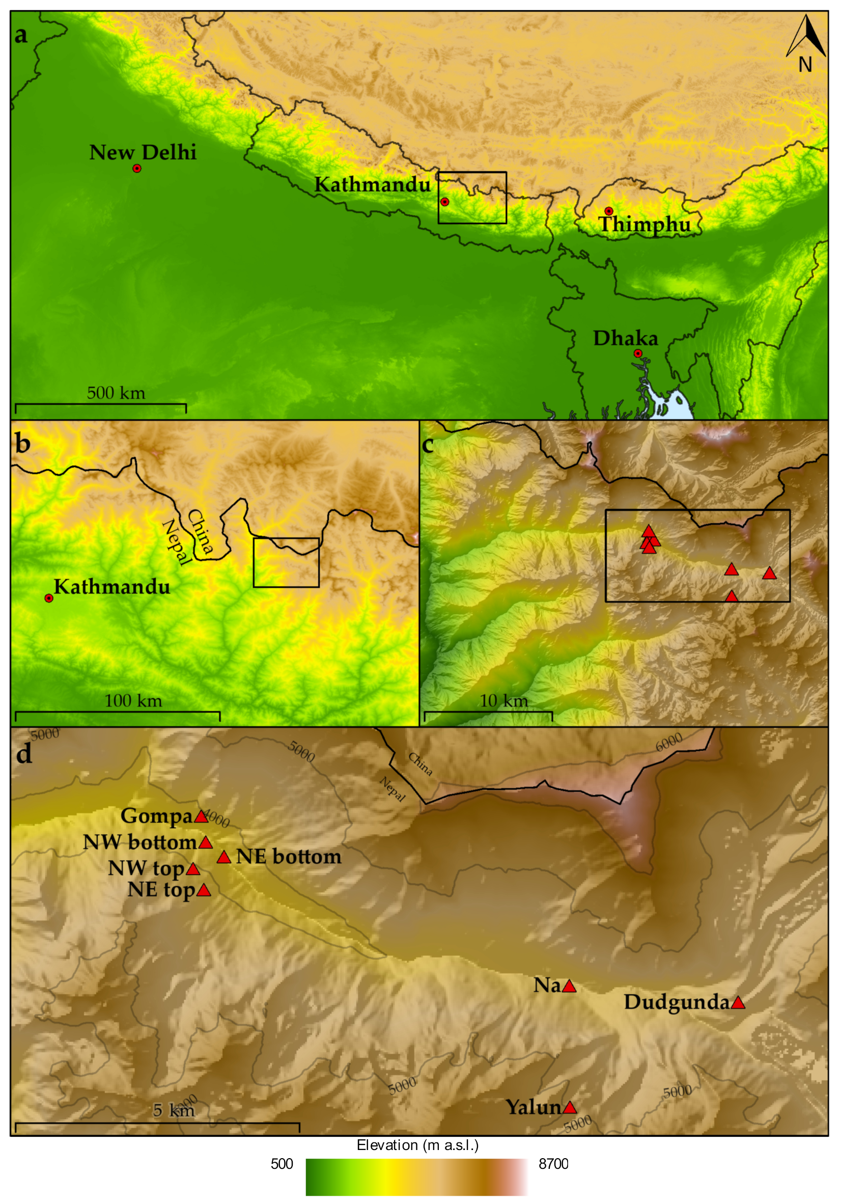
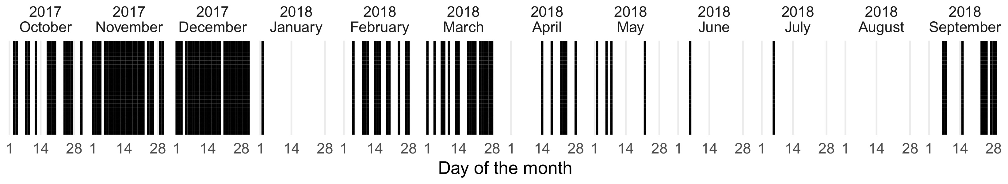
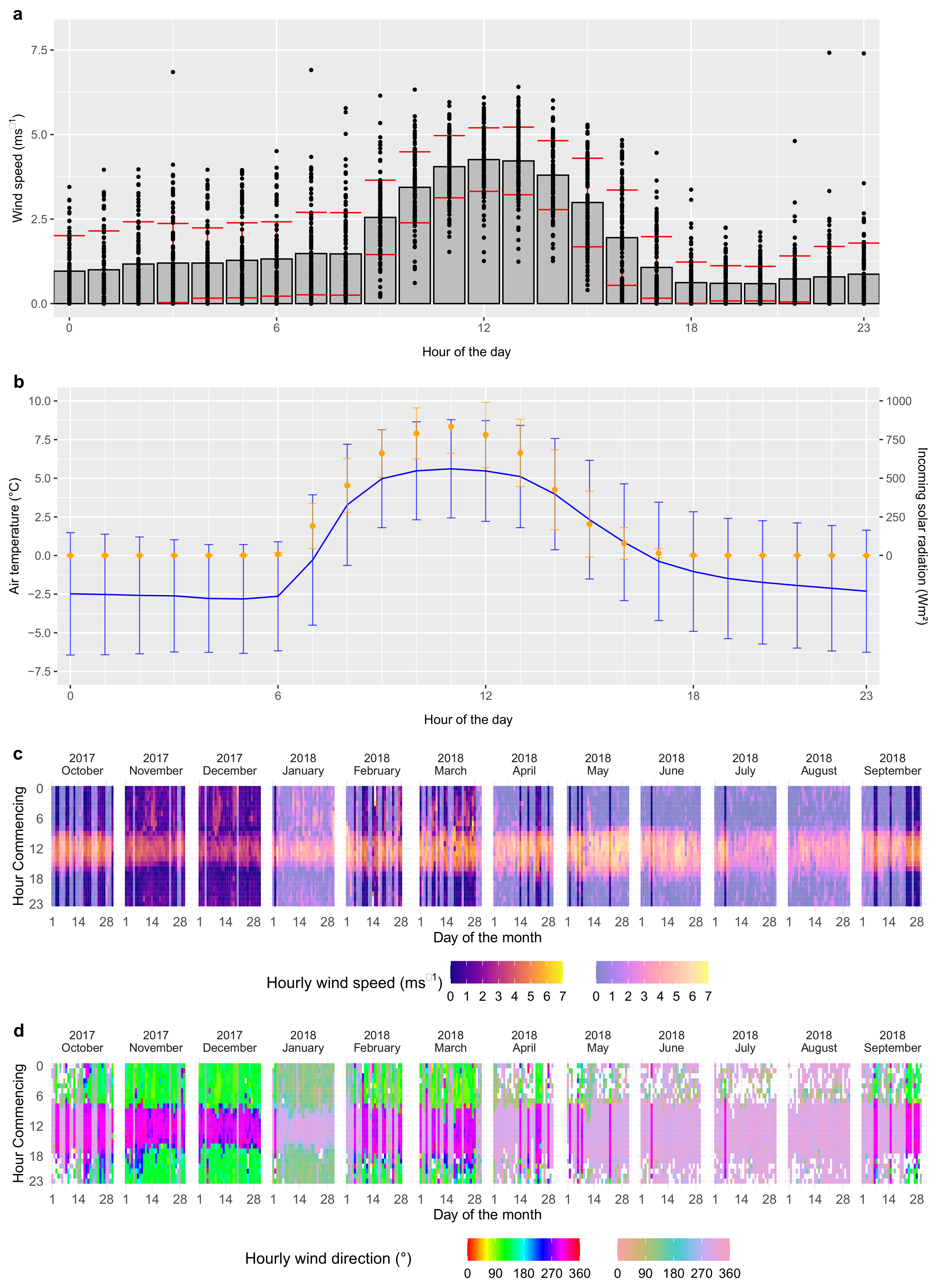
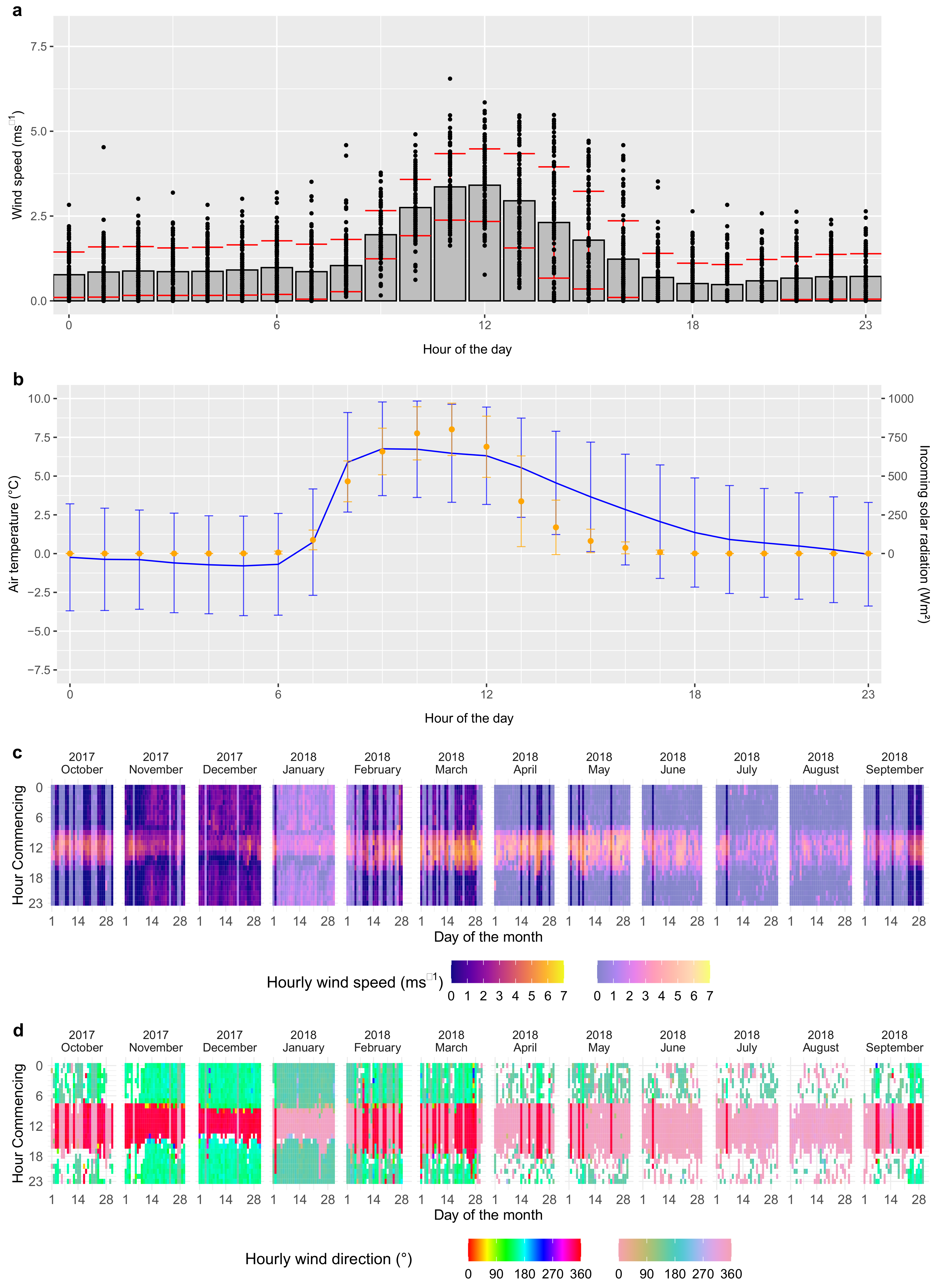
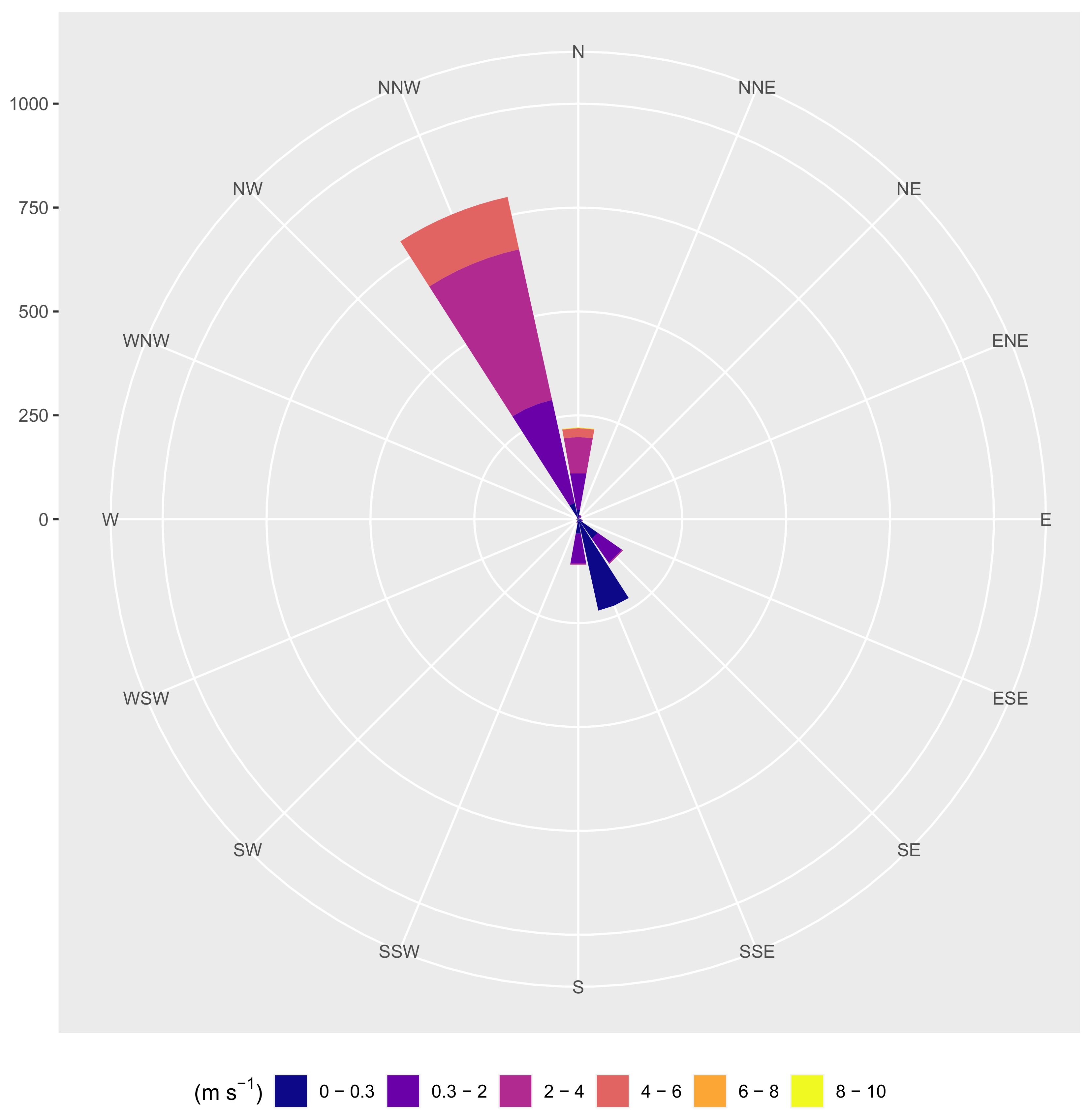
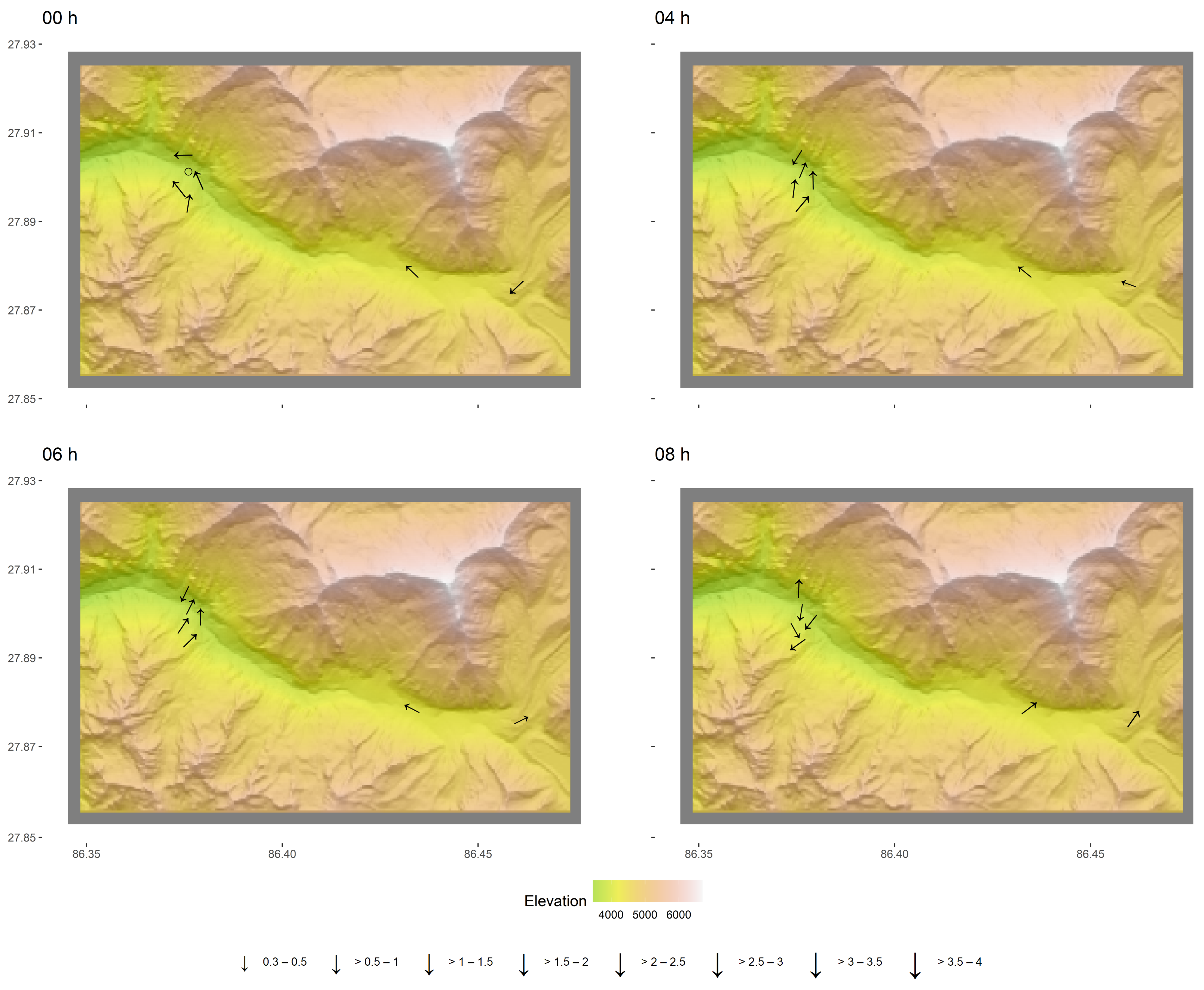
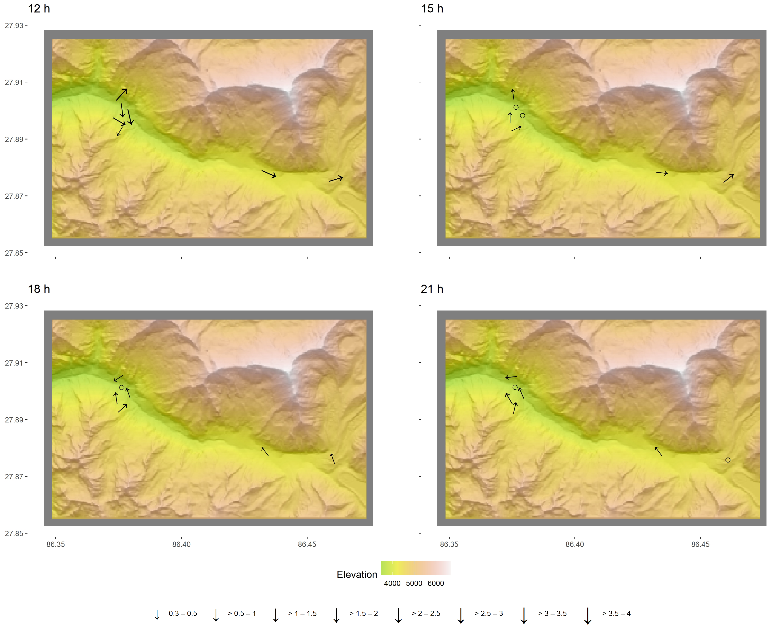
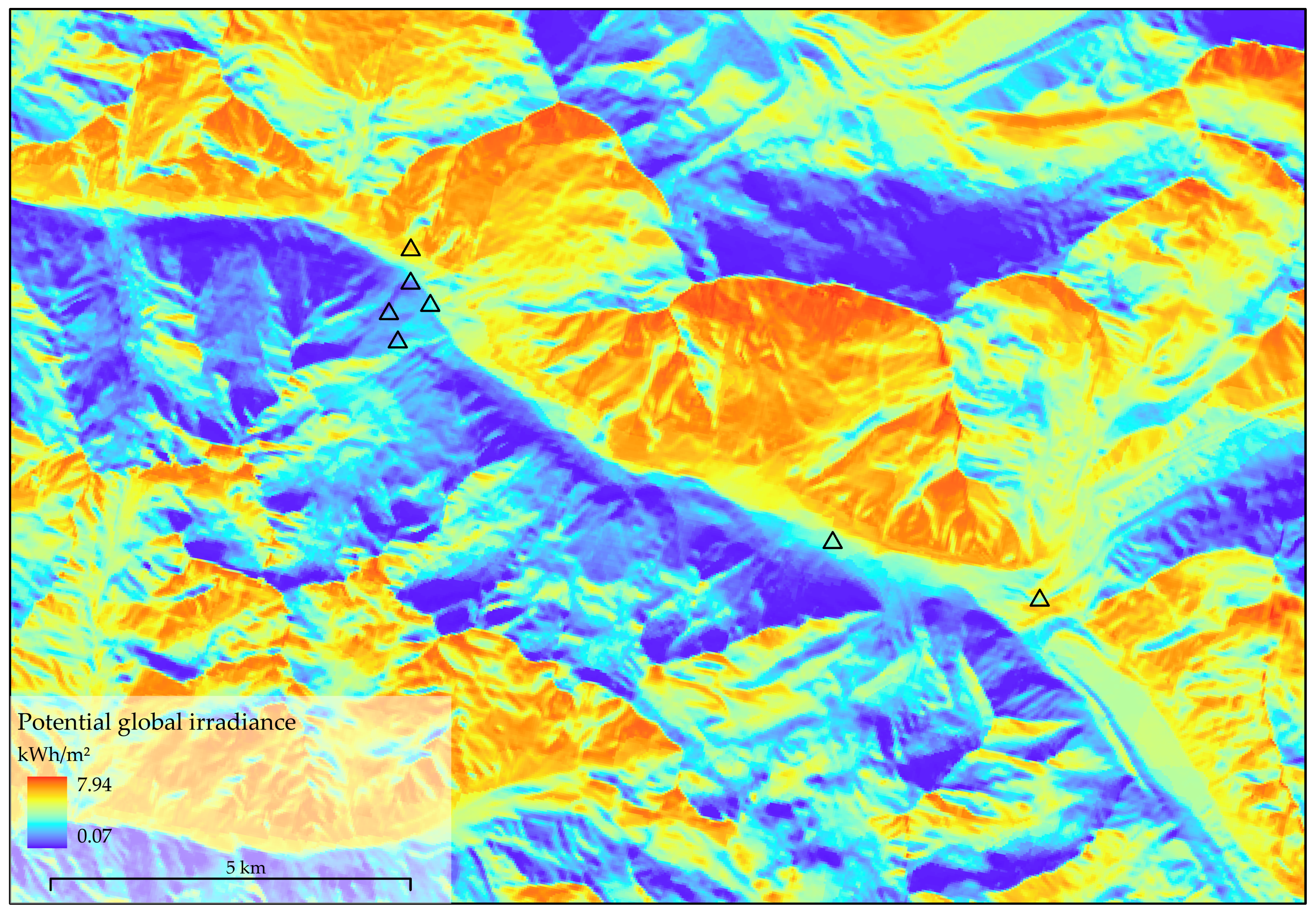
Table 1.
Automated weather station (AWS) in the TREELINE station network [9]. Mean hourly wind speeds were calculated within the period of 1 October 2017 to 30 September 2018.
Table 1.
Automated weather station (AWS) in the TREELINE station network [9]. Mean hourly wind speeds were calculated within the period of 1 October 2017 to 30 September 2018.
| Station | Latitude (N) | Longitude (E) | Elevation (m a.s.l.) | Position | Mean Hourly Wind Speed (m s) |
|---|---|---|---|---|---|
| NW bottom | 27.9009 | 86.3762 | 3718.9 | Valley floor | 0.62 |
| NE bottom | 27.8986 | 86.3791 | 3734.2 | Valley floor | 1.08 |
| Na | 27.8782 | 86.4337 | 4192.1 | Valley floor | 1.66 |
| Dudgunda | 27.8756 | 86.4604 | 4532.2 | Valley floor | 1.25 |
| Gompa | 27.9050 | 86.3755 | 3886.0 | Slope | 0.94 |
| NW top | 27.8967 | 86.3742 | 4035.9 | Slope | 1.46 |
| NE top | 27.8934 | 86.3759 | 4158.3 | Slope | 1.14 |
| Yalun | 27.8590 | 86.4338 | 5005.2 | Slope | — |
Table 2.
Sensor properties according to the manufacturer Onset Computer Corporation, Bourne, MA 02532, USA [61].
Table 2.
Sensor properties according to the manufacturer Onset Computer Corporation, Bourne, MA 02532, USA [61].
| Sensor Type | Sensor ID | Measurement Range | Operating Range | Other Details |
|---|---|---|---|---|
| Weather station data logger | U30-NRC | −40–60 C | Logging interval: 15 min (user defined), storage capacity: 512 Kb flash storage | |
| Wind speed | S-WSB-M003 | 0–76 m s, accuracy: ±1.1 m s or ±4%, automatic averaging | −40–75 C | Starting threshold: 1 m s horizontal movement |
| Wind direction | S-WDA-M003 | 0–355, 5 dead band, accuracy: ±5, unit vector averaging | −40–70 C | Starting threshold: 1 m s resolution: 1.4 horizontal movement |
| Solar radiation | S-LIB-M003 | −1280 W m, Accuracy: ±10 W m, Drift: <±2% per year | −40–75 C | ±0.38 W m error at conditions >25 C, Spectral range: 300–1100 nm |
| Temperature | S-THB-M008 | −40–75 C, accuracy: ±0.02 from 0–50 C, drift: <0.1 C per year | −40–75 C | |
| Rain gauge | S-RGB-M002 | 0–12.7 cm h, Max. 4000 tips per logging interval, accuracy: ±1.0 at 20 mm h | 0–50 C | Resolution: 0.2 mm |
Publisher’s Note: MDPI stays neutral with regard to jurisdictional claims in published maps and institutional affiliations. |
© 2022 by the authors. Licensee MDPI, Basel, Switzerland. This article is an open access article distributed under the terms and conditions of the Creative Commons Attribution (CC BY) license (https://creativecommons.org/licenses/by/4.0/).
Share and Cite
MDPI and ACS Style
Jentsch, H.; Weidinger, J. Spatio-Temporal Analysis of Valley Wind Systems in the Complex Mountain Topography of the Rolwaling Himal, Nepal. Atmosphere 2022, 13, 1138. https://0-doi-org.brum.beds.ac.uk/10.3390/atmos13071138
AMA Style
Jentsch H, Weidinger J. Spatio-Temporal Analysis of Valley Wind Systems in the Complex Mountain Topography of the Rolwaling Himal, Nepal. Atmosphere. 2022; 13(7):1138. https://0-doi-org.brum.beds.ac.uk/10.3390/atmos13071138
Chicago/Turabian StyleJentsch, Helge, and Johannes Weidinger. 2022. "Spatio-Temporal Analysis of Valley Wind Systems in the Complex Mountain Topography of the Rolwaling Himal, Nepal" Atmosphere 13, no. 7: 1138. https://0-doi-org.brum.beds.ac.uk/10.3390/atmos13071138
Note that from the first issue of 2016, this journal uses article numbers instead of page numbers. See further details here.