Data-Driven Prediction of COVID-19 Daily New Cases through a Hybrid Approach of Machine Learning Unsupervised and Deep Learning

Abstract

Air pollution is associated with respiratory diseases and the transmission of infectious diseases. In this context, the association between meteorological factors and poor air quality possibly contributes to the transmission of COVID-19. Therefore, analyzing historical data of particulate matter (PM${}_{2.5}$ and PM${}_{10}$) and meteorological factors in indoor and outdoor environments to discover patterns that allow predicting future confirmed cases of COVID-19 is a challenge within a long pandemic. In this study, a hybrid approach based on machine learning and deep learning is proposed to predict confirmed cases of COVID-19. On the one hand, a clustering algorithm based on K-means allows the discovery of behavior patterns by forming groups with high cohesion. On the other hand, multivariate linear regression is implemented through a long short-term memory (LSTM) neural network, building a reliable predictive model in the training stage. The LSTM prediction model is evaluated through error metrics, achieving the highest performance and accuracy in predicting confirmed cases of COVID-19, using data of PM_2.5 and PM₁₀ concentrations and meteorological factors of the outdoor environment. The predictive model obtains a root-mean-square error (RMSE) of 0.0897, mean absolute error (MAE) of 0.0837, and mean absolute percentage error (MAPE) of 0.4229 in the testing stage. When using a dataset of PM_2.5, PM₁₀, and meteorological parameters collected inside 20 households from 27 May to 13 October 2021, the highest performance is obtained with an RMSE of 0.0892, MAE of 0.0592, and MAPE of 0.2061 in the testing stage. Moreover, in the validation stage, the predictive model obtains a very acceptable performance with values between 0.4152 and 3.9084 for RMSE, and a MAPE of less than 4.1%, using three different datasets with indoor environment values.

1. Introduction

The COVID-19 pandemic caused by the agent of severe acute respiratory syndrome coronavirus (SARS-CoV-2) has generated many deaths worldwide; at the end of May 2022, the total is approximately 6 million in the world and 325,000 thousand in Mexico, with confirmed cases of around 528 million and 5.78 million, respectively [1]. The COVID-19 pandemic tested the organization, protocols, processes, and care and response time of the healthcare system in all countries. The World Health Organization (WHO) issued recommendations and protocols to reduce the spread of the virus [2]. Governments, international institutions, public and private laboratories, and research centers have worked on developing vaccines to control the spread of the virus, reduce the risks to the patient’s health, and prevent death in the event of infection. The rapid spread of SARS-CoV-2 caused the closure of industrial, commercial, agricultural, educational, and investment activities in different pandemic waves, causing a deterioration of the global economy, which encouraged a home office scheme in a wide variety of businesses.

Several studies have reported a possible relationship between air pollution and meteorological factors with the transmission of COVID-19 [3,4,5,6,7]. These studies have analyzed data on the concentrations of pollution, meteorological parameters, and confirmed cases during the lockdown and partial lockdown of the COVID-19 pandemic. Therefore, indoor and outdoor air quality can play an important role in the transmission of SARS-CoV-2. In this sense, the Centers for Disease Control and Prevention (CDC) describes that people become infected with SARS-CoV-2 through exposure to respiratory fluids that carry the infectious virus [8]. This can occur by inhalation of very fine respiratory droplets and aerosol particles, deposition of respiratory droplets and particles on mucous membranes (mouth, nose, and eyes) by splashing or direct aerosols, or by contact of the mucous membrane with hands contaminated with contaminated respiratory fluids or touching surfaces infected with the virus [8].

Exposure to indoor pollutants is one of the main contributors to total human exposure, causing respiratory, cardiovascular, lung cancer, and allergic diseases in prolonged exposures [9,10]. These indicators of contamination are very relevant since human beings spend around 90% of their time in closed environments [11]. Indoor air pollution ranks in the top five environmental risks to public health [12]. Occupants of indoor environments are exposed to various pollutants, such as particulate matter (PM${}_{2.5}$ and PM${}_{10}$), carbon monoxide (CO), carbon dioxide (CO₂), nitrogen oxides (NO_x), volatile organic compounds (VOCs), ozone (O₃), and bio-aerosols [13]. During the confinement implemented to reduce the growth curve of COVID-19 infections, the social distancing restrictions increased the home occupancy and home-office activities. Nowadays, changes have been reported in levels of pollutants inside homes [14,15,16,17,18], and outdoor pollution has decreased in many cities [19,20,21,22,23].

Fine particulate matter with a size of less than 2.5 μm (PM_2.5) is considered one of the most significant environmental risks to people’s health. Long-term exposure to particulate matter pollution (PM${}_{2.5}$ and PM${}_{10}$) is associated with a high rate of respiratory illness and hospitalizations for chronic lung disease, pneumonia, cerebrovascular diseases, schematic heart disease, lung cancer, and mortality [24,25,26,27]. An association between PM${}_{2.5}$ and confirmed cases, deaths, and hospital admissions due to COVID-19 infections has been proven in several regions affected by the pandemic [28,29,30,31,32,33]. Furthermore, several studies have estimated a relationship between short- and long-term exposure to PM${}_{10}$ with confirmed cases of COVID-19 [34,35,36], patients who experienced pneumonia due to COVID-19 [37], and COVID-19 severity and mortality [38,39]. Therefore, the COVID-19 pandemic has highlighted the need to reduce particle concentrations to low levels through public policies to reduce risks to the population’s health due to short-term and long-term exposure to air pollutants, which includes the spread of SARS-CoV-2.

The pandemic’s impact on a global level (mental health, personal health, economy, business, and interpersonal relationships) has required the implementation of mathematical, statistical, and computational methods to discover patterns that allow the identification of possible behaviors in the spread of COVID-19. Deep-learning techniques have been proposed to classify X-ray images of people infected with COVID-19 [40,41,42,43], predict confirmed cases and deaths [44,45], identify people’s moods through social networks analysis [46,47], and diagnose and treat COVID-19 [48], among others.

In this study, an approach based on unsupervised machine learning and deep learning is proposed to predict confirmed cases of COVID-19, using historical data on pollution by PM${}_{2.5}$, PM${}_{10}$ and meteorological factors in the indoor and outdoor environment, as well as confirmed cases and deaths from COVID-19. The data were collected during the third wave of COVID-19 in Victoria, Mexico. The datasets were examined to identify a possible structure in the values of the multidimensional variables using the Andrews curves method. Furthermore, the datasets were analyzed using an unsupervised K-means clustering algorithm to discover behavior patterns by forming highly cohesive groups. Subsequently, a multivariate linear regression analysis from the discovered clusters was implemented through a deep-learning long short-term memory (LSTM) neural network. The predictive model is evaluated through the root-mean-square error (RMSE), the mean absolute error (MAE), the mean square error (MSE), and the mean absolute percentage error (MAPE) metrics.

2. Materials and Methods

2.1. Area of Study

This study was conducted in the city of Victoria (23°44′00″ N 99°08′00″ W), located in the State of Tamaulipas in northeastern Mexico, which had a population of approximately 350,000 inhabitants in 2020 within an approximate area of 188 km². The population density per km² in 2020 was 1845 inhabitants. The annual mean temperature (2021) was 25.3 °C, with a minimum and maximum temperature of 0 °C and 42 °C, respectively. The data on the concentration of ambient air pollutants and meteorological factors in outdoor environments were collected through four monitoring stations. These stations are installed in commercial, residential, downtown, and suburban areas at the neighborhood level, considering the topographical conditions of the city, located next to a mountainous area.

2.2. Data Collection

The outdoor environmental pollution data used in the study are from 1 May to 31 October 2021. Raw data were downloaded from a private cloud on the Internet, which contains a database that receives and stores the data collected by the four monitoring stations. These stations transmit the values collected by the sensors in real time, with a temporal resolution of 24 h/7 days. When the data are received in the cloud, they are automatically processed, validated, and saved using a cloud service. The outdoor dataset contains hourly average values for PM${}_{2.5}$ ($\mathsf{\mu }$g/m³), PM${}_{10}$ ($\mathsf{\mu }$g/m³), temperature (°C), relative humidity (%), atmospheric pressure (hPa), wind speed (Km/h), and wind direction (°). Each monitoring station has a low-cost sensor (LCS) for particulate matter 9387-P, marketed by Libelium. This sensor is based on the Alphasense OPC-N3 sensor, which uses a laser beam to count particles, detecting particles from 0.35 $\mathsf{\mu }$m to 40 $\mathsf{\mu }$m, sorting them into 24-size containers capable of measuring up to 2000 $\mathsf{\mu }$g/m³ (PM${}_{2.5}$), with a maximum coincidence probability of 0.84% at 10,000,000 particles/L, and 0.24% at 500 particles/L [49]. In our experiment, particulate matter LCS (9387-P) was calibrated locally before each study, achieving a determination coefficient of $R^2$ = 0.86 for PM${}_{2.5}$ and $R^2$ = 0.75 for PM${}_{10}$ with the reference instrument.

The indoor air pollution data were collected between 27 May and 13 October 2021. A total of 20 households were selected in which at least one inhabitant was diagnosed positive in a COVID-19 test. The mobile indoor monitoring station was installed 15 days after the house inhabitants obtained a negative COVID-19 test result. In addition, the house was required to be disinfected by the public health department or by a private company authorized by the government. The indoor dataset stores mean values of the attributes PM${}_{2.5}$ ($\mathsf{\mu }$g/m³), PM${}_{10}$ ($\mathsf{\mu }$g/m³), temperature (°C), relative humidity (%), and atmospheric pressure (hPa) collected inside the houses. Furthermore, we added the values of the wind speed (Km/h) and wind direction (°) attributes collected at the monitoring station closest to the household to the dataset. The measurements were conducted for 7 day/24 h continuously indoors at 3-min intervals. The monitoring equipment was placed at approximately a 1.3 m height indoors; depending on the time of day, it was located for several hours in the kitchen, dining room/living room, or bedroom (this action was performed by the person who lives in the house). The indoor monitoring instrument was equipped with a Plantower PMS7003 LCS [50]. The manufacturer guarantees accuracy for PM${}_{2.5}$ (similar accuracy for PM${}_{10}$) of 10 $\mathsf{\mu }$g/m³ in the range 0–100 $\mathsf{\mu }$g/m³, 10% for measurements in the range 101–500 $\mathsf{\mu }$g/m³, and 20% over concentration 500 $\mathsf{\mu }$g/m³. The particulate matter LCS (PMS7003) was calibrated before the study period, obtaining a correlation coefficient of $R^2$ = 0.90 for PM${}_{2.5}$ and $R^2$ = 0.78 for PM${}_{10}$ with the reference instrument. Temperature and relative humidity were measured with a BOSCH BME280 sensor [51], with a temperature measurement range of −40 °C to 85 °C, an atmospheric pressure range of 300 to 1100 hPa with a sensitivity error of ±0.25%, and relative humidity with an accuracy of ±3% RH and hysteresis ≤2% RH. Each of the 20 monitored homes are located relatively close to an outdoor monitoring station; that is, 5 of the monitored homes are located nearby each monitoring station. On the one hand, 16 homes are located in low-income areas, ventilation is natural by opening windows and the homes have at least one pedestal fan. On the other hand, four homes are located in middle-income areas; ventilation is hybrid, through air conditioning equipment installed in the bedroom or living room and natural ventilation through opening windows. Furthermore, at least one pedestal or ceiling fan is available in these homes.

The number of confirmed cases and deaths from COVID-19 recorded in Victoria city from 27 May to 13 October 2021, and were compiled from the COVID-19 Mexico website (open access data) of the government of Mexico. We built a dataset with the number of confirmed cases and deaths per day. These attributes were added to the outdoor air pollutants and meteorological factors dataset.

2.3. Statistical Analysis

Daily confirmed cases and deaths from COVID-19, concentration levels of pollutants in the air, and indoor and outdoor meteorological parameters were statistically analyzed using the Kolmogorov–Smirnov Lilliefors test to determine the normality of the data. The datasets were identified as non-parametric distribution, for which it was determined to apply a Spearman correlation analysis independently for indoor and outdoor pollution. Spearman’s correlation coefficient was used to examine the relationship between variables considered in our study. A clustering analysis based on K-means was implemented, allowing us to discover behavior patterns between the instances of the indoor/outdoor datasets, confirmed cases, and deaths from COVID-19, through the formation of natural groups in the feature space. A multivariate linear regression analysis was performed using a deep learning architecture based on an LSTM neural network from the clusters discovered. In the training phase of the LSTM neural network, the prediction model with the highest accuracy rate was selected, which allows for predicting future COVID-19 confirmed cases with high efficiency and performance. In addition, a descriptive analysis was performed by calculating the median, interquartile range (IQR), minimum and maximum values for the continuous variables of concentrations of air pollutants, and meteorological factors.

The R language over the RStudio IDE (version 1.3.959) was used to perform the data distribution Kolmogorov–Smirnov test and the descriptive statistical analysis. The k-means clustering analysis was performed using the Scikit-Learn tool (version 1.1.1). The datasets were standardized because they contained variables at different scales using the StandardScaler library installed on the Scikit-Learn tool. Standardization is a pre-processing task on the dataset, allowing the building of a deep learning model. Multivariate linear regression using the LSTM neural network was implemented on a Jupyter Notebook, using Python Keras 2.6.0, the high-level deep learning neural network library, with the TensorFlow 2.6.0 backend. Furthermore, the CuDNN library for LSTM networks (CuDNNLSTM) was implemented for faster execution in the training and testing stages of the LSTM model, reducing computation time using GPU technology. CuDNN is a GPU-accelerated library of primitives for deep neural networks.

Table 1. Parameters of the LSTM neural network.

Layer	Parameter
LSTM	700 units
Activation	tanh
recurrent_activation	sigmoid
unroll	False
use_bias	True
recurrent_dropout	0
return_sequences	True
TimeDistributed Dense	1
optimizer	adamax
loss	mae
epochs	300
batch_size	32

shows the hyper-parameters defined in the LSTM neural network model. The Pandas 1.2.4 framework was implemented to manage the datasets and handle the neural network’s time series. Moreover. the Plotly 5.1.0 library was implemented to generate the visualization of the results through graphs.

3. Results

3.1. Statistic Analysis

The p-value given by the Kolmogorov–Smirnov Lilliefors test is less than 0.05 for both datasets (D = 0.24532 and D = 0.2397 for outdoor and indoor datasets, respectively), meaning that, indeed, the data is not normally distributed. The median PM${}_{2.5}$ concentration registered is between 12 $\mathsf{\mu }$g/m³ and 16 $\mathsf{\mu }$g/m³, with an IQR between 10 $\mathsf{\mu }$g/m³ and 22 $\mathsf{\mu }$g/m³, in the different monitored areas of the city (see

Table 2. Descriptive statistics of meteorological factor data and particulate matter concentration outdoors.

Station	PM${}_{2.5}$ ($\mathsf{\mu }$g/m3)			PM${}_{10}$ ($\mathsf{\mu }$g/m3)			Temperature (°C)			Relative Humidity (%)
	Median (IQR)	Min	Max	Median (IQR)	Min	Max	Median	Min	Max	Median	Min	Max
AQIoT-2	12 (10)	3	76	14 (12)	4	86	27.3	16.2	42.0	88.7	41.1	99.8
AQIoT-3	12 (14)	4	274	13 (15)	5	330	27.3	15.7	41.8	86.4	35.4	99.9
AQIoT-4	16 (22)	5	621	18 (25)	6	636	27.4	16.1	42.0	86.0	40.4	99.8
AQIoT-5	13 (14)	3	87	14 (15)	4	99	27.2	15.3	41.5	90.9	29.7	99.9

). The maximum level for PM${}_{2.5}$ was recorded at the AQIoT-4 station (621 $\mathsf{\mu }$g/m³), and 636 $\mathsf{\mu }$g/m³ for PM${}_{10}$, which occurred during the forest fire season at the beginning of August (summer season). At the AQIoT-3 station, a median PM${}_{10}$ of 13 $\mathsf{\mu }$g/m³ was registered, and a PM${}_{10}$ of 18 $\mathsf{\mu }$g/m³ at the AQIoT-4 station during the study period. In this period, the minimum temperature of 15.3 °C was recorded in the first week of October 2021 (autumn season) at the AQIoT-5 monitoring station, which is located near the mountain area (see Table 2). Relative humidity was reported with minimums of 29% to 41% in late spring and summer, with a maximum of 99% recorded during the rainy season (September and October).

The reference value standard in Mexico is defined as 30 $\mathsf{\mu }$g/m³ for PM${}_{2.5}$ and 50 $\mathsf{\mu }$g/m³ for PM${}_{10}$ for a 24-h average, published by the Ministry of Health of the Government of Mexico in the environmental health norm [52]. In this context, the AQIoT-2 station PM${}_{2.5}$ daily mean exceeded the official norm on October 13 and 14 (33.9 $\mathsf{\mu }$g/m³ and 37.75 $\mathsf{\mu }$g/m³). At the AQIoT-3 station, the norm was exceeded on several days with a mean PM${}_{2.5}$ concentration of 37.88 $\mathsf{\mu }$g/m³ (July 18), 32.24 $\mathsf{\mu }$g/m³ (1 September), and 34.68 $\mathsf{\mu }$g/m³, 38.20 $\mathsf{\mu }$g/m³, 41.18 $\mathsf{\mu }$g/m³, and 32.84 $\mathsf{\mu }$g/m³ from 12 October to 15 October, respectively. At the AQIoT-4 station, the greatest number of days with concentrations outside the permissible limits for PM${}_{2.5}$ and PM${}_{10}$ occurred. The following levels for PM${}_{2.5}$ were recorded: 48.15 $\mathsf{\mu }$g/m³ on 18 Jul, from 19 August to 31 August, levels between 43.77 $\mathsf{\mu }$g/m³ and 258.72 $\mathsf{\mu }$g/m³, on September 1, 32.56 $\mathsf{\mu }$g/m³, and 36.97 $\mathsf{\mu }$g/m³, 39.75 $\mathsf{\mu }$g/m³, 44.64 $\mathsf{\mu }$g/m³, and 35.37 $\mathsf{\mu }$g/m³ from 12 October to 15 October, respectively. PM${}_{10}$ concentrations exceeded the environmental health norm with 62.19 $\mathsf{\mu }$g/m³ (18 July), 76.80 $\mathsf{\mu }$g/m³ to 259.46 $\mathsf{\mu }$g/m³ from 19 August to 31 August and on 14 October with a 56.12 $\mathsf{\mu }$g/m³ level. Finally, at the AQIoT-5 station, the PM${}_{2.5}$ limit was exceeded with levels of 33.37 $\mathsf{\mu }$g/m³ (1 September) and between 31.48 $\mathsf{\mu }$g/m³ to 42.73 $\mathsf{\mu }$g/m³ from 12 October to 15 October and 51.74 $\mathsf{\mu }$g/m³ for PM${}_{10}$ on 14 October 2021.

On the other hand, in the descriptive analysis for particulate matter data inside the houses, the lowest median of 8(11) $\mathsf{\mu }$g/m³ was recorded in households located near the AQIoT-4 station (see

Table 3. Descriptive statistics of meteorological parameters data, and indoor concentration of particulate matter (PM${}_{2.5}$ and PM${}_{10}$).

Station	PM${}_{2.5}$ ($\mathsf{\mu }$g/m3)			PM${}_{10}$ ($\mathsf{\mu }$g/m3)			Temperature (°C)			Relative Humidity (%)
	Median (IQR)	Min	Max	Median (IQR)	Min	Max	Median	Min	Max	Median	Min	Max
AQIoT-2	21 (19)	2	223	23 (21)	3	230	34.8	28.8	39.4	57.2	33.9	95.0
AQIoT-3	15 (17)	3	177	16 (18)	4	177	34.8	21.4	39.6	56.5	35.6	93.9
AQIoT-4	8 (11)	2	311	9 (11)	3	365	33.6	28.4	36.5	58.6	38.7	91.2
AQIoT-5	14 (16)	2	141	16 (17)	3	143	33.9	28.4	37.9	62.6	36.5	90.4

), and the highest median of 21(19) $\mathsf{\mu }$g/m³ at the AQIoT-2 station. PM${}_{10}$ levels follow this pattern of these stations with 9(11) $\mathsf{\mu }$g/m³ and 23(21) $\mathsf{\mu }$g/m³, respectively. The maximum for PM${}_{2.5}$ pollution was registered in 311 $\mathsf{\mu }$g/m³ and for PM${}_{10}$ in 365 $\mathsf{\mu }$g/m³. The activities may influence these values carried out in the kitchen and the filtration of pollutants from the outside. In addition, most of the monitored houses do not have a cooker hood installed on the stove that allows the extraction of particles generated when cooking food and by the combustion of liquefied petroleum gas (butane/propane) used for cooking food. The maximum temperature recorded inside the houses was very high (from 37.9 °C to 39.6 °C), with an average temperature between 33.6 °C to 34.8 °C in the monitored areas (see Table 3). These temperatures occurred between 3:00 p.m. and 9:00 p.m., from May to August 2021, coinciding with minimums of 33.9% to 38.7% relative humidity.

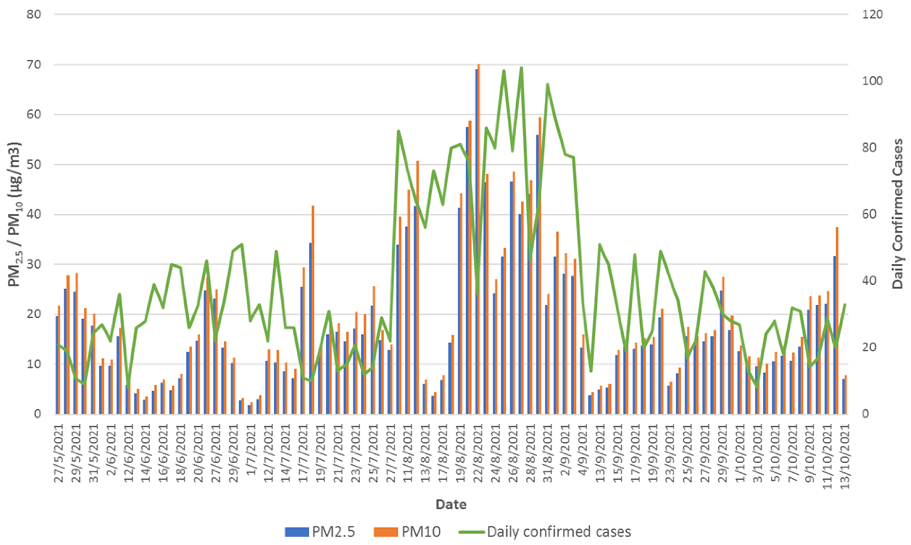
The accumulated confirmed cases during the study period were 5981 people with a positive test (53% are female patients), with a daily maximum of 104 confirmed cases of COVID-19. Figure 1 shows the daily increase in infected people reported by the Ministry of Public Health between 1 May and 31 October 2021. On the other hand, in the study period, 138 deaths caused by complications from COVID-19 were reported (63% correspond to male patients), with a cumulative of 571 deaths since initiating the process of confinement for the pandemic (17 March 2020).

Figure 2 and Figure 3 show the mean daily concentration of PM${}_{2.5}$ and PM${}_{10}$ in outdoor and indoor air, respectively, and the number of COVID-19 cases recorded per day. Figure 2 shows that on several days in August 2021, the 24 h standard average (30 $\mathsf{\mu }$g/m³) for PM${}_{2.5}$ was exceeded, coinciding with the period in which the highest number of COVID-19 confirmed cases per day were recorded. In the case of the pollutant PM${}_{10}$, the short-term standard (50 $\mathsf{\mu }$g/m³) for daily average was exceeded on four occasions during the same month.

Furthermore, Spearman correlation analysis was used to decipher the relationships between confirmed COVID-19 cases, particulate matter ambient air pollutants concentrations, and five meteorological variables.

Table 4. Spearman correlation coefficient matrix using the outdoor pollution and meteorological factors dataset.

	PM${}_{2.5}$	PM${}_{10}$	T	RH	WD	WS	AP	DCC	Deaths
PM${}_{\mathbf{2.5}}$	1	1 **	0.56 *	−0.39	0.11	−0.15	0.24	−0.74 **	−0.25
PM${}_{\mathbf{10}}$	1 **	1	0.59 *	−0.42	0.14	−0.16	0.23	−0.74 **	−0.25
T	0.56 *	0.59 *	1	−0.70 **	0.64 **	−0.07	0.14	−0.36	0.04
RH	−0.39	−0.42	−0.70 **	1	−0.39	0.29	0.00	0.33	0.02
WD	0.11	0.14	0.64 **	−0.39	1	0.42	0.19	−0.15	0.32
WS	−0.15	−0.16	−0.07	0.29	0.42	1	0.19	0.03	0.35
AP	0.24	0.23	0.14	0.00	0.19	0.19	1	−0.27	0.49 *
DCC	−0.74 **	−0.74 **	−0.36	0.33	−0.15	0.03	−0.27	1	0.02
Deaths	−0.25	−0.25	0.04	0.02	0.32	0.35	0.49 *	0.02	1

* p-value > 0.05, ** p-value > 0.01.

shows Spearman’s coefficient matrix calculated using the dataset of particulate matter and meteorological factors in outdoor air. This analysis aims to identify the behavior and association between the study variables, considering the growth in positive cases and deaths for COVID-19 in these 20 weeks. All particulate matter types showed perfect positive correlation with each other, r = 1 (p-value < 0.01). Statistically moderate positive correlations between PM${}_{2.5}$ and temperature (T) and PM${}_{10}$ and T were found at a significant level of 5% (0.56 ≥ r ≤ 0.59). We found that PM${}_{2.5}$ and PM${}_{10}$ have a strong negative correlation for daily confirmed cases (DCC) of COVID-19, with a coefficient value of −0.74 (p-value < 0.01) in both associations. Furthermore, results show a moderate correlation coefficient of atmospheric pressure and deaths for COVID-19 at 0.49, with a p-value of less than 0.05. The correlation analysis reveals a negative coefficient between the relative humidity (RH) and T (r = −0.70, p-value < 0.01). We observe that T exhibits a strong relationship (r = 0.64, p-value < 0.01) with wind direction (WD) variable.

On the other hand,

Table 5. Spearman correlation coefficient matrix using the indoor pollution and meteorological parameters dataset.

	PM${}_{2.5}$	PM${}_{10}$	T	RH	WD	WS	AP	DCC	Deaths
PM${}_{\mathbf{2.5}}$	1.00	0.99 **	−0.53 **	0.48 *	0.15	−0.05	−0.17	0.50 *	0.40 *
PM${}_{\mathbf{10}}$	0.99 **	1.00	−0.50 *	0.49 *	0.11	−0.06	−0.20	0.48 *	0.40 *
T	−0.53 **	−0.50 *	1.00	−0.60 **	−0.35	0.19	−0.18	−0.13	−0.15
RH	0.48 *	0.49 *	−0.60 **	1.00	−0.12	−0.60 **	−0.08	0.11	0.32
WD	0.15	0.11	−0.35	−0.12	1.00	0.69 **	0.33	0.23	−0.14
WS	−0.05	−0.06	0.19	−0.60 **	0.69 **	1.00	0.08	0.12	−0.08
AP	−0.17	−0.20	−0.18	−0.08	0.33	0.08	1.00	−0.29	−0.33
DCC	0.50 *	0.48 *	−0.13	0.11	0.23	0.12	−0.29	1.00	0.22
Deaths	0.40 *	0.40 *	−0.15	0.32	−0.14	−0.08	−0.33	0.22	1.00

* p-value > 0.05, ** p-value > 0.01.

shows the Spearman correlation matrix computed for the indoor dataset. In this second correlation scenario, the concentration of pollutants and meteorological parameters for the 20 households and the confirmed cases and deaths from COVID-19 in the study’s period were considered. The correlation coefficient between PM${}_{2.5}$ and PM${}_{10}$ was highlighted as very high with r = 0.99 and the p-value < 0.01, as well as a moderate association between PM${}_{2.5}$ and PM${}_{10}$ with the temperature (T) variable with r = 0.53 and r = 0.50, respectively. Furthermore, we found a moderate relationship between relative humidity (RH) and the two types of particulate matter, with a significance level of less than 0.05. The variables corresponding to the meteorological parameters present strong correlations. Temperature and relative humidity show a correlation coefficient of r = 0.60 (p-value < 0.01). In addition, a strong positive correlation between wind direction (WD) and the variable wind speed (WS) with r = 0.69 (p-value < 0.01), as well as a negative association between relative humidity and wind speed of r= −0.60, p-value < 0.01. Finally, the correlation between PM${}_{2.5}$ and PM${}_{10}$ with the daily confirmed cases (DCC) of COVID-19 shows important changes with respect to the level of correlation found in the outdoor scenario: a moderate positive correlation of r = 0.50 between PM${}_{2.5}$ and confirmed cases and a relationship between PM${}_{10}$ and confirmed cases of r = 0.48 (p-value < 0.05). Furthermore, in this scenario, we find a moderate positive correlation between the particulate matter variables and COVID-19 deaths, with r = 0.40 and p-value < 0.05, in both cases.

3.2. Dataset Analysis

Before implementing the machine learning algorithm based on K-means clustering, the datasets were analyzed to identify if there is a structure in the behavior of the values of the multidimensional variables. Visualizing multidimensional data is a complex process compared to visualizing data in two or three dimensions. Then, implementing the Andrews curves method, one can identify the dataset structure since complex data is reduced to a two-dimensional graph, making it possible to specify the associated variables, the formation of groups, and outliers within the dataset. The curves are created using the features of instances of each dataset as coefficients of the Fourier series.

Figure 4 shows the graph of the Andrews curves generated by comparing the outdoor data of air pollution and meteorological factors with the indoor data of air pollution and meteorological parameters. In this Figure, each color represents a class (indoor/outdoor); it can be seen that the lines that represent the instances of the same class have similar curves. Furthermore, a similarity between the curves of the two classes is identified. In addition, it is observed that the vast majority of the data has a structure of sinusoidal curves with which a pattern is discovered in the data, which makes it possible to apply an automatic learning algorithm to discover this structure and understand the equation behind its data. The Andrews plot shows the areas where the classes are grouped and correlated (for example, on the X-axis with a value of 1.1 and between −300 and −1200 on the Y-axis. Similarly, a correlation between classes can be seen in the value 2 on the X-axis and between the values 700 and 1500 on the Y-axis). On the other hand, some atypical values are observed in the outdoor class (gray lines), for example; in the curve located at the value of 0.2 on the X-axis with the value of 1750 on the Y-axis. In values 2.2 and 1750 corresponding to the X-axis and Y-axis, other outliers occur in the same class. In addition, atypical values are observed in the indoor class (green lines), which are displayed correlated with atypical values of the outdoor class throughout the plot, for example, in the line located at the value −2 of the X-axis with the value −250 of the Y-axis.

In Figure 5, four classes corresponding to outdoor air quality monitoring stations (AQIoT-2, AQIoT-3, AQIoT-4, and AQIoT-5) were defined to discover if the data from the four monitoring stations share a data structure and follow a pattern. This Figure shows the data structure using the Andrews curves method; it identified that it has a similar structure and is consistent with the data structure and patterns discovered in Figure 4. In addition, the same types of outliers are identified, and most belong to the AQIoT-4 monitoring station (purple lines). It is observed that some of these outliers correlate with values from the AQIoT-2 monitoring station (gray lines). These two monitoring stations are located in the southeast and northeast areas of the city, with a linear distance of approximately 5 km, and share similar characteristics of altitude above sea level, topographical conditions, and wind currents. This correlation is visualized in the lines at the value −2 on the X-axis and between −200 and −350 on the Y-axis.

Figure 6 shows the indoor air pollution data structure for which 20 classes were defined and represent the data collected in the 20 monitored houses. At the level of detail displayed in Figure 6, it is observed that in the data structure in the rise of the curve located at the value −2 of the X-axis (between the values 700 and 1000 of the Y-axis) until the descent before the curve located at the value −1 of the X-axis (between the values −850 and −1300 of the Y-axis) there is an almost perfect grouping of the lines, which continues at the end of this curve and until the beginning of the next curve. A group between fewer classes but with a correlation between all classes is visualized in the following curves. Regarding the outliers, it is identified that the house labeled with class 17 correlates with the outliers identified for outdoor class (see Figure 4). This discovery is important because household 17 is close to the AQIoT-4 monitoring station (see outliers in Figure 5).

3.3. Clustering Analysis

The K-means clustering algorithm was used to classify the instances of all variables in each dataset. The K-means algorithm is an unsupervised method of grouping by partitions; it does not require a class or prior knowledge to classify an instance within a group or cluster based on a measure of similarity between samples. In our approach, the algorithm was implemented using the Euclidean distance metric, selecting the instances with the minimum distance to the centroid ($C_k$); that is, there is maximum homogeneity between the objects in the group and the greatest difference between the groups. The number of clusters (K) was defined by implementing the Elbow method, which allows for determining the optimal value for K. In the three datasets used in our experiment, this method determined an optimal value of $K=3$, using all the variables and instances in each dataset. In addition, the value of the initial centroids was defined randomly, considering all the instances of the dataset.

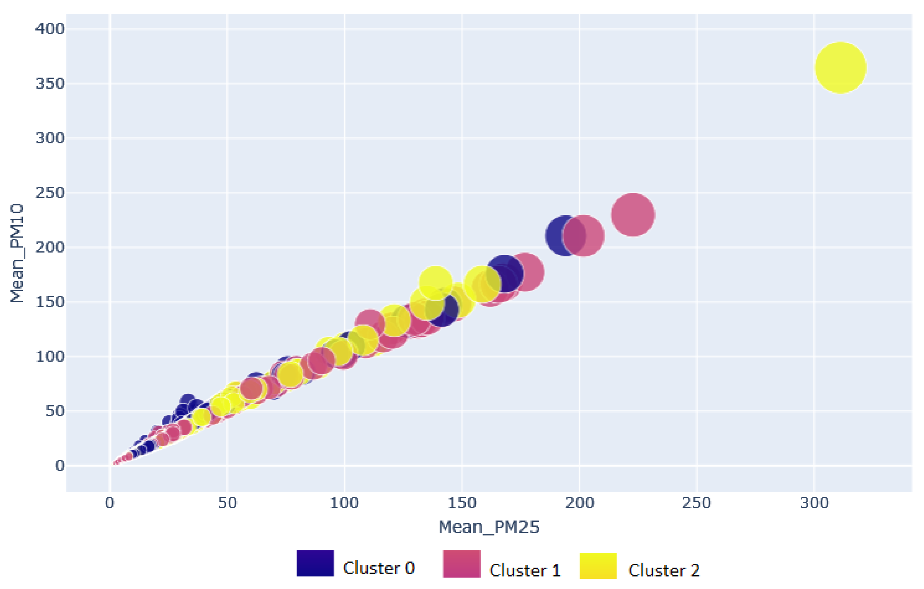
The clustering analysis will allow identifying the groups that contain more instances and the origin of these instances (indoor or outdoor, monitoring station or homes), enabling us to find a representative group that allows training the LSTM neural network model with high performance and predict with the minimum error future cases of people infected by COVID-19. Figure 7 shows the result of the clustering analysis considering the dataset divided into indoor and outdoor environments. Cluster 0 is the most populated with 3643 instances, followed by clusters 2 and 1 with 3547 and 2789. Most cluster 0 instances belong to the AQIoT-4 monitoring station or the houses located near this station and are linked to the AQIoT-4 monitoring station; the same scenario is presented in cluster 2. The goodness of the clustering obtained was evaluated through the silhouette coefficient (also known as silhouette width), obtaining a value of Si = 0.61; a value in the Si > 0 means that the observation is well grouped; the closer it is to 1, the better the grouping. The silhouette coefficient allows interpreting and validating the coherence between the group elements; that is, it measures how similar an object is within its group (cohesion) compared to other groups (separation).

Figure 8 shows the clusters generated for the outdoor type dataset divided by a monitoring station. Cluster 1 has the largest number of instances (2910); in cluster 0, 2829 homogeneous instances are grouped. In cluster 1 and cluster 2, most samples correspond to the AQIoT-3 monitoring station, followed by AQIot-4 with a minimum difference of six instances. AQIoT-4 is the most representative in instances grouped in cluster 0. In the grouping validation, the model outdoor type dataset obtained an average silhouette width of Si = 0.62.

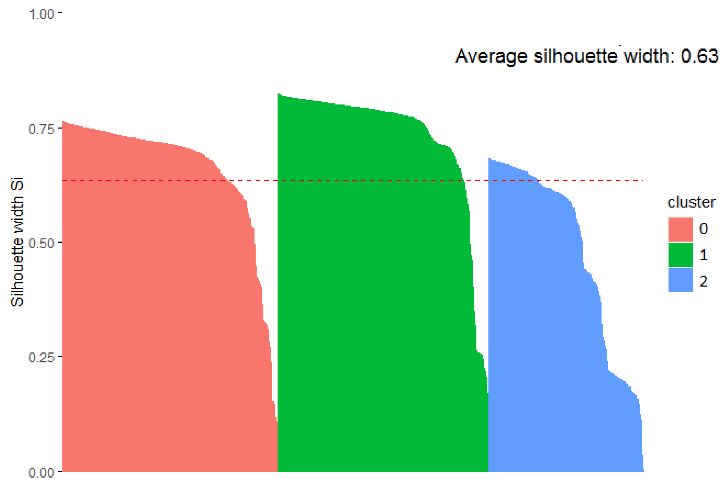
The cluster analysis, using the data collected inside houses presents a behavior similar to that displayed in the cluster analysis for indoor–outdoor and outdoor datasets. The similarity is observed in the formation of the clusters, the clusters with more instances, and the origin of the instances (linkage to a monitoring station). Figure 9 shows the formation of the clusters using the indoor data; some instances with greater distance to the centroid of their cluster are observed for which they are shown separated from the group. The clusters generated from the indoor data obtained the best goodness evaluation compared to the previously presented clusters, with a Si = 0.63, as shown in Figure 10.

3.4. Prediction Model

Instances labeled with the AQIoT-4 monitoring station identifier were extracted from the indoor and outdoor datasets, generating two new datasets. In each of these datasets, 80% of the instances were selected to build a sub-dataset (for each dataset) that will be used in the training of the LSTM neural network, which allows generating a prediction model based on LSTM for each dataset (indoor/outdoor). The remaining 20% of instances of the original dataset were built into the test sub-dataset and used to evaluate the prediction model’s performance. In the training stage, the LSTM model learns from the behavior (dependency between variables) identified from the regression analysis of each instance in the training dataset. The number of confirmed cases is the target or dependent variable (output) and is a function of independent variables or predictors (input). In our experiment, the predictors are PM${}_{2.5}$, PM${}_{10}$, temperature, relative humidity, atmospheric pressure, wind speed, and wind direction. Then, with the predictive model generated in the training stage, each instance of the test dataset is used to predict the value per day of the confirmed cases variable. In each prediction, the LSTM model receives the value of the eight predictor variables as input.

Table 6. Error metrics results of LSTM deep learning model during testing and validation stages (outdoor dataset).

Station	% of Instances	RMSE	MAE	MSE	MAPE
AQIoT-2	100%	0.2560	0.1397	0.0655	0.4196
AQIoT-3	100%	0.2523	0.1483	0.0637	0.4310
AQIoT-4	20%	0.0897	0.0837	0.0080	0.4229
AQIoT-5	100%	0.2386	0.1508	0.0569	0.5070

shows the performance obtained by the LSTM prediction model using the outdoor dataset. First, the prediction model is evaluated with the remaining 20% of the AQIoT-4 monitoring station dataset instances. The prediction model obtains error metrics very close to 0. The RMSE metric reaches a value of 0.0897, indicating the concentration level of the data in the regression line has an excellent fit, with a minimum distance from the data points of the regression line. Furthermore, the difference between the predicted and actual values is low, with an MAE of 0.0837, indicating that the average forecast is very acceptable. Regarding the MAPE metric, a value reached 0.4229 suggests that the average difference between the predicted and current values is less than 1%.

The LSTM prediction model was validated with 100% of the dataset instances from the AQIoT-2, AQIoT-3, and AQIoT-5 monitoring stations. An RMSE metric of 0.2560 was obtained with the first dataset (see Table 6), indicating an average distance between the predicted values of confirmed cases of COVID-19 by the model and the real values in the validation dataset. Moreover, the prediction model obtained an MAE = 0.2560, an MSE = 0.0655, and a MAPE = 0.4196, reporting a high accuracy of the regression model in the prediction. Similarly, in the validation of the prediction model with the datasets of the monitoring stations AQIoT-3 and AQIoT-5, very acceptable error metrics were achieved, 0.2523 and 0.2386 in the RMSE and MAE of 0.1483 and 0.1508, respectively. In the validation stage with the outdoor data collected at the AQIoT-5 station, the model obtained the highest MAPE error metric for the prediction task (0.5070).

Figure 11 shows the comparison of the time series between the actual data (blue line) and the predicted data (red line), with a prediction of 85 days of confirmed cases of COVID-19, using 100% of the dataset on particulate matter and meteorological factors collected at the AQIoT-2 monitoring station (outdoor). Figure 11 shows a similar prediction between the real (original) value and the predicted value; only in the forecast between days 40 and 42 (X-axis) is there a slight separation between predicted and real data. On days 46, 48, 51, and 83, a prediction slightly lower than the real value is observed. Figure 12 shows the prediction of confirmed cases of COVID-19 generated from the AQIoT-4 station test dataset. The predicted data is for 16 days, without observing a difference between the predicted data line and the real data. This is because the difference between the number of confirmed cases predicted and the number of confirmed cases contained in the test dataset is at the decimal level (for example, 6.148918 vs. 6), which is confirmed by the metrics of very low errors achieved by the deep learning LSTM network model.

Table 7. Error metrics results of the LSTM neural network model during testing and validation stages (indoor dataset).

Station	% of Instances	RMSE	MAE	MSE	MAPE
Houses near AQIoT-2	100%	0.4152	0.3243	0.1724	1.7302
Houses near AQIoT-3	100%	3.9084	1.1627	15.2756	4.0744
Houses near AQIoT-4	20%	0.0892	0.0592	0.0079	0.2061
Houses near AQIoT-5	100%	1.5046	1.0603	2.2641	1.7082

presents the performance of the LSTM prediction model for confirmed cases of COVID-19, using PM${}_{2.5}$, PM${}_{10}$ concentration data and meteorological parameters collected inside houses as input data to the model. The neural network LSTM was trained with 80% of the instances of the indoor dataset linked (located near) to the AQIoT-4 monitoring station. The remaining 20% of the dataset was used to test the prediction model. Moreover, the predictive model was validated with 100% of the three datasets containing particulate matter concentration and meteorological factor values in five households (indoor) each. These houses are located near the AQIoT-2, AQIoT-3, and AQIoT-5 monitoring stations, respectively. The validation of the prediction model using the dataset of houses near the AQIoT-2 monitoring station obtained a very acceptable performance with very low error metrics, with values of 0.4152, 0.3243, and 0.1724, in RMSE, MAE, and MSE, and with a value in the MAPE metric less than 2%. In the validation with data from houses near the AQIoT-3 station, the highest error metrics of the model were reached, with an RMSE = 3.9084, an MAE = 1.1627, and a MAPE of 4.0744 (see Table 7). These metrics are acceptable since the prediction model adjusts to unknown values and complex behaviors in the input data and manages to predict confirmed cases of COVID-19 with error metrics of less than 5%. The minor error metrics in the testing and validation stages of the predictive model were obtained with the dataset of houses near the AQIoT-4 monitoring station, with values of 0.0892, 0.0592, and 0.2061 for RMSE, MAE, and MAPE, respectively, confirming the high performance and accuracy of the predictive model (see Table 7). When the model was validated with the dataset of houses near the AQIoT-5 monitoring station, an RMSE = 1.5046, a MAPE of less than 2%, and an MAE value of 1.0603 were obtained, demonstrating that the predicted data are very close to actual data.

Figure 13 and Figure 14 show the predictions of confirmed cases of COVID-19 using the pollution values by particulate matter (PM${}_{2.5}$ and PM${}_{10}$) and meteorological parameters inside houses located around the monitoring stations AQIoT-3 and AQIoT-5. With these datasets, the prediction model reached the highest values in the error metrics in its validation stage (see Table 7). In the predicted data shown in the time series of Figure 13, a different behavior than expected is identified on day 4, with a predicted value lower than the actual value (8.12 versus 26). Subsequently, the behavior is similar between the real and the predicted data, with a slightly smaller difference between the predicted data and the original data on days 12, 16, 18, and 20. In the time series shown in Figure 14, the predicted data line follows the behavior discovered in the real data. However, in the prediction of the second day, it has a value slightly higher than expected. In contrast, from day 13 to day 22, it predicts slightly lower than expected values in the number of confirmed cases.

4. Discussion

Models to predict new infections, deaths, and recovered patients from COVID-19 have been a topic of great interest to the scientific community in recent months [53,54]. The authors of [55] propose a multivariate and univariate model based on a Stacked LSTM network for forecasting the time series of COVID-19 deaths in Sao Paulo. Data from the air quality index, temperature, and relative humidity, as well as the number of confirmed cases and deaths from COVID-19, are used to train the LSTM network. In the evaluation stage of the predictive model, it reached an RMSE of 8.62, considering the variables of deaths from COVID-19 and the air quality index to predict deaths from COVID-19. In [56], the authors evaluate various methods based on machine learning to predict the spread of COVID-19, concluding that the variables of humidity and temperature have a greater weight than other variables in predicting the mortality rate.

For their part [57], they propose the use of a multilayer perceptron (MLP) neural network to implement a regression model with the capacity to determine the relationship between the parameters of pollutants in the air and the number of COVID-19 patients, estimating the number of patients corresponding to each parameter of the contaminant. This study uses data on the concentrations of PM${}_{10}$, PM${}_{2.5}$, SO₂, NO_x, NO₂, O₃, CO, and confirmed cases of patients with COVID-19. The implemented model obtains a rate of 97% in the testing stage of the prediction performed. In [58], they use three variants of the LSTM neural network to predict daily cases of COVID-19. In the multivariate regression approach, they use the values of relative humidity and temperature to improve the model’s performance, which is implemented with data from different cities. The predictive model obtains the best results in the multivariate proposal with an RMSE between 0.175 and 142.112 and a MAPE between 0.6 and 8.9, considering diverse populations. Tsan et al. [59], present an approach based on the LSTM neural network to predict confirmed cases of COVID-19. The proposed model can predict confirmed cases in ranges of 1, 3, 7, and 14 days. In the proposal, values of five air pollutants and seven meteorological factors are combined with the number of confirmed cases of COVID-19 to build a dataset. The predictive model obtains a performance (using all the variables of the dataset) according to the RMSE metric of 66.697, 80.617, 71.526, and 75.965 for the predictions of 1, 3, 7, and 14 days, respectively.

Nowadays, diverse approaches have been proposed that associate meteorological variables, air pollution, and confirmed cases and deaths of COVID-19. Researchers seek to determine a relationship between these variables that allows finding patterns in the data to build reliable prediction models. An important aspect during the confinement implemented through various social distancing rules due to the COVID-19 pandemic in the world is indoor air pollution. Our proposal deals with data-driven analysis based on the pollution levels of PM${}_{2.5}$ and PM${}_{10}$ inside houses where at least one inhabitant was infected with some variant of COVID-19. The predictive model is based on an unsupervised machine learning and deep learning approach. The predictive model obtained low error metrics in the testing and validation stages using pollution data and indoor meteorological parameters. In the test stage, the predictive model achieves an RMSE value of 0.0892 and a MAPE of 0.2061, using only 20% of the instances in the dataset. In the validation stage, it reaches an RMSE of 0.4152 and a MAPE of 1.7302 in one of the three datasets used in this stage. The prediction model obtained higher error metrics when data collected inside houses near the AQIoT-3 and AQIoT-5 monitoring stations were used (see Table 7). Therefore, we must consider that the concentration of PM${}_{2.5}$ and PM${}_{10}$ variability inside the monitored houses increases the complexity of the problem. This variability is caused by the different activities carried out inside the households. For example, the concentration levels in the kitchen increase when food is cooked and by the combustion of propane/butane gas. However, in these houses, the variation in temperature and relative humidity is minimal when carrying out these activities in the kitchen area. In the study, these activities vary in duration and timetable in which they are carried out, and each house is an environment with specific characteristics (for example, number of windows, people who live in the house, air extraction system, etc.) that can affect the behavior of the pollutants in a certain period. An additional explanation is that the number of confirmed cases time series has a medium linear correlation with the daily mean concentration of PM${}_{2.5}$ and PM${}_{10}$ time-series; in terms of the LSTM neural network training stage, this does not add lots of information in the search space.

On the other hand, the proposed approach was also implemented considering outdoor pollution data of PM${}_{2.5}$, PM${}_{10}$, and meteorological factors, associating these variables with confirmed cases and deaths from COVID-19 in the same period. The LSTM predictive model obtains very high performance and accuracy in the test stage with an RMSE of 0.0897 and a MAPE of 0.4229. In the validation stage, the model reaches RMSE values of 0.2386, 0.2523, and 0.2560, and in the MAPE metric of 0.4196, 0.4310, and 0.5070 for the three datasets used in this stage, respectively. With the error metrics presented, it is possible to trust the predictive model based on the LSTM neural network due to its performance and accuracy in the testing and validation stages.

5. Conclusions

In this paper, we verify the influence of particulate matter concentrations (PM${}_{2.5}$ and PM${}_{10}$) and meteorological factors (relative humidity, temperature, atmospheric pressure, wind direction, and speed) on the spread of COVID-19. The association between these variables made it possible to predict future positive cases of COVID-19 from data collected in Victoria, Mexico. In our proposal, the LSTM neural network predictive model was trained with particulate matter pollution data and meteorological factors from outside and inside houses. The outdoor dataset corresponds to the data collected through four monitoring stations at the residential level. The indoor dataset was generated from data collected inside 20 households distributed near the monitoring stations. A k-means clustering algorithm was implemented to discover patterns from the cluster formation. The above allows selecting the ideal dataset to train the LSTM neural network model. The predictive model implements a multivariate linear regression obtaining very low error metrics (with both datasets). Then, it can be considered a viable and reliable option due to its performance and accuracy in predicting the number of confirmed cases of COVID-19, based on particulate matter concentration data and meteorological factors.

References

1. World Health Organization. WHO Coronavirus (COVID-19) Dashboard. 2022. Available online: https://covid19.who.int/ (accessed on 31 May 2022).
2. WHO World Health Organization. Report of the WHO-China Joint Mission on Coronavirus Disease 2019 (COVID-19). 2022. Available online: https://www.who.int/emergencies/diseases/novel-coronavirus-2019/situation-reports (accessed on 7 January 2021).
3. Zhang, X.; Tang, M.; Guo, F.; Wei, F.; Yu, Z.; Gao, K.; Jin, M.; Wang, J.; Chen, K. Associations between air pollution and COVID-19 epidemic during quarantine period in China. Environ. Pollut. 2021, 268, 115897. [Google Scholar] [CrossRef] [PubMed]
4. Setti, L.; Passarini, F.; De Gennaro, G.; Barbieri, P.; Perrone, M.G.; Borelli, M.; Palmisani, J.; Di Gilio, A.; Torboli, V.; Fontana, F.; et al. SARS-Cov-2RNA found on particulate matter of Bergamo in Northern Italy: First evidence. Environ. Res. 2020, 188, 109754. [Google Scholar] [CrossRef]
5. Sangkham, S.; Thongtip, S.; Vongruang, P. Influence of air pollution and meteorological factors on the spread of COVID-19 in the Bangkok Metropolitan Region and air quality during the outbreak. Environ. Res. 2021, 197, 111104. [Google Scholar] [CrossRef]
6. Zhao, C.; Fang, X.; Feng, Y.; Fang, X.; He, J.; Pan, H. Emerging role of air pollution and meteorological parameters in COVID-19. J. Evid.-Based Med. 2021, 14, 123–138. [Google Scholar] [CrossRef] [PubMed]
7. Xu, L.; Taylor, J.E.; Kaiser, J. Short-term air pollution exposure and COVID-19 infection in the United States. Environ. Pollut. 2022, 292, 118369. [Google Scholar] [CrossRef]
8. National Center for Immunization and Respiratory Diseases (NCIRD), Division of Viral Diseases. CDC COVID-19 Science Briefs [Internet]. Atlanta (GA): Centers for Disease Control and Prevention (US); Scientific Brief: SARS-CoV-2 Transmission. 2020. Available online: https://0-www-ncbi-nlm-nih-gov.brum.beds.ac.uk/books/NBK570442/ (accessed on 17 March 2022).
9. Ferreira, A.; Barros, N. COVID-19 and Lockdown: The Potential Impact of Residential Indoor Air Quality on the Health of Teleworkers. Int. J. Environ. Res. Public Health 2022, 19, 6079. [Google Scholar] [CrossRef]
10. Kakoulli, C.; Kyriacou, A.; Michaelides, M.P. A Review of Field Measurement Studies on Thermal Comfort, Indoor Air Quality and Virus Risk. Atmosphere 2022, 13, 191. [Google Scholar] [CrossRef]
11. Mannan, M.; Al-Ghamdi, S.G. Indoor Air Quality in Buildings: A Comprehensive Review on the Factors Influencing Air Pollution in Residential and Commercial Structure. Int. J. Environ. Res. Public Health 2021, 18, 3276. [Google Scholar] [CrossRef]
12. EPA—Environmental Protection Agency. Why Indoor Air Quality is Important to Schools. 2020. Available online: https://www.epa.gov/iaq-schools/why-indoor-air-quality-important-schools (accessed on 24 March 2022).
13. González-Martín, J.; Kraakman, N.J.R.; Pérez, C.; Lebrero, R.; Muñoz, R. A state–of–the-art review on indoor air pollution and strategies for indoor air pollution control. Chemosphere 2021, 262, 128376. [Google Scholar] [CrossRef] [PubMed]
14. Tahmasebi, F.; Wang, Y.; Cooper, E.; Shimizu, D.G.; Stamp, S.; Mumovic, D. Window operation behaviour and indoor air quality during lockdown: A monitoring-based simulation-assisted study in London. Build. Serv. Eng. Res. Technol. 2022, 43, 5–21. [Google Scholar] [CrossRef]
15. Domínguez-Amarillo, S.; Fernández-Agüera, J.; Cesteros-García, S.; González-Lezcano, R.A. Bad Air Can Also Kill: Residential Indoor Air Quality and Pollutant Exposure Risk during the COVID-19 Crisis. Int. J. Environ. Res. Public Health 2020, 17, 7183. [Google Scholar] [CrossRef] [PubMed]
16. Algarni, S.; Khan, R.A.; Khan, N.A.; Mubarak, N.M. Particulate matter concentration and health risk assessment for a residential building during COVID-19 pandemic in Abha, Saudi Arabia. Environ. Sci. Pollut. Res. Int. 2021, 28, 65822–65831. [Google Scholar] [CrossRef]
17. Roh, T.; Moreno-Rangel, A.; Baek, J.; Obeng, A.; Hasan, N.T.; Carrillo, G. Indoor Air Quality and Health Outcomes in Employees Working from Home during the COVID-19 Pandemic: A Pilot Study. Atmosphere 2021, 12, 1665. [Google Scholar] [CrossRef]
18. Ninyà, N.; Vallecillos, L.; Marcé, R.M.; Borrull, F. Evaluation of air quality in indoor and outdoor environments: Impact of anti-COVID-19 measures. Sci. Total Environ. 2022, 836, 155611. [Google Scholar] [CrossRef]
19. Chen, B.; Huang, Y.; Huang, J.; Dong, L.; Guan, X.; Ge, J.; Hu, Z. Using Lidar and Historical Similar Meteorological Fields to Evaluate the Impact of Anthropogenic Control on Dust Weather During COVID-19. Front. Environ. Sci. 2021, 9, 806094. [Google Scholar] [CrossRef]
20. Lovrić, M.; Pavlović, K.; Vuković, M.; Grange, S.K.; Haberl, M.; Kern, R. Understanding the true effects of the COVID-19 lockdown on air pollution by means of machine learning. Environ. Pollut. 2021, 274, 115900. [Google Scholar] [CrossRef]
21. Briz-Redón, Á.; Belenguer-Sapiña, C.; Serrano-Aroca, Á. Changes in air pollution during COVID-19 lockdown in Spain: A multi-city study. J. Environ. Sci. 2021, 101, 16–26. [Google Scholar] [CrossRef]
22. Anil, I.; Alagha, O. The impact of COVID-19 lockdown on the air quality of Eastern Province, Saudi Arabia. Air Qual. Atmos. Health 2021, 14, 117–128. [Google Scholar] [CrossRef]
23. Dong, L.; Chen, B.; Huang, Y.; Song, Z.; Yang, T. Analysis on the Characteristics of Air Pollution in China during the COVID-19 Outbreak. Atmosphere 2021, 12, 205. [Google Scholar] [CrossRef]
24. Cohen, A.J.; Brauer, M.; Burnett, R.; Anderson, H.R.; Frostad, J.; Estep, K.; Balakrishnan, K.; Brunekreef, B.; Dandona, L.; Dandona, R.; et al. Estimates and 25-year trends of the global burden of disease attributable to ambient air pollution: An analysis of data from the Global Burden of Diseases Study 2015. Lancet 2017, 389, 1907–1918. [Google Scholar] [CrossRef]
25. Rhee, J.; Dominici, F.; Zanobetti, A.; Schwartz, J.; Wang, Y.; Di, Q.; Balmes, J.; Christiani, D.C. Impact of Long-Term Exposures to Ambient PM2.5 and Ozone on ARDS Risk for Older Adults in the United States. Chest 2019, 156, 71–79. [Google Scholar] [CrossRef] [PubMed]
26. Liu, C.; Chen, R.; Sera, F.; Vicedo-Cabrera, A.M.; Guo, Y.; Tong, S.; Coelho, M.S.; Saldiva, P.H.; Lavigne, E.; Matus, P.; et al. Ambient Particulate Air Pollution and Daily Mortality in 652 Cities. N. Engl. J. Med. 2019, 381, 705–715. [Google Scholar] [CrossRef] [PubMed]
27. Domingo, J.L.; Rovira, J. Effects of air pollutants on the transmission and severity of respiratory viral infections. Environ. Res. 2020, 187, 109650. [Google Scholar] [CrossRef] [PubMed]
28. Coker, E.S.; Cavalli, L.; Fabrizi, E.; Guastella, G.; Lippo, E.; Parisi, M.L.; Pontarollo, N.; Rizzati, M.; Varacca, A.; Vergalli, S. The Effects of Air Pollution on COVID-19 Related Mortality in Northern Italy. Environ. Resour. Econ. 2020, 76, 611–634. [Google Scholar] [CrossRef]
29. Ali, S.M.; Malik, F.; Anjum, M.S.; Siddiqui, G.F.; Anwar, M.N.; Lam, S.S.; Nizami, A.S.; Khokhar, M.F. Exploring the linkage between PM2.5 levels and COVID-19 spread and its implications for socio-economic circles. Environ. Res. 2021, 193, 110421. [Google Scholar] [CrossRef]
30. Adhikari, A.; Yin, J. Short-Term Effects of Ambient Ozone, PM2.5, and Meteorological Factors on COVID-19 Confirmed Cases and Deaths in Queens, New York. Int. J. Environ. Res. Public Health 2020, 17, 4047. [Google Scholar] [CrossRef]
31. Chakrabarty, R.K.; Beeler, P.; Liu, P.; Goswami, S.; Harvey, R.D.; Pervez, S.; van Donkelaar, A.; Martin, R.V. Ambient PM2.5 exposure and rapid spread of COVID-19 in the United States. Sci. Total Environ. 2021, 760, 143391. [Google Scholar] [CrossRef]
32. Mendy, A.; Wu, X.; Keller, J.L.; Fassler, C.S.; Apewokin, S.; Mersha, T.B.; Xie, C.; Pinney, S.M. Air pollution and the pandemic: Long-term PM2.5 exposure and disease severity in COVID-19 patients. Respirology 2021, 26, 1181–1187. [Google Scholar] [CrossRef]
33. Lym, Y.; Kim, K.J. Exploring the effects of PM2.5 and temperature on COVID-19 transmission in Seoul, South Korea. Environ. Res. 2022, 203, 111810. [Google Scholar] [CrossRef]
34. Mangla, S.; Pathak, A.K.; Arshad, M.; Ghosh, D.; Sahoo, P.K.; Garg, V.K.; Haque, U. Impact of Environmental Indicators on the COVID-19 Pandemic in Delhi, India. Pathogens 2021, 10, 1003. [Google Scholar] [CrossRef]
35. Cartenì, A.; Cascetta, F.; Di Francesco, L.; Palermo, F. Particulate Matter Short-Term Exposition, Mobility Trips and COVID-19 Diffusion: A Correlation Analyses for the Italian Case Study at Urban Scale. Sustainability 2021, 13, 4553. [Google Scholar] [CrossRef]
36. Babak, K.; Kiarash, F.; Hannaneh, T.; Reza, M. Association between short-term exposure to air pollution and COVID-19 hospital admission/mortality during warm seasons. Environ. Monit. Assess. 2021, 193, 426. [Google Scholar] [CrossRef]
37. Pegoraro, V.; Heiman, F.; Levante, A.; Urbinati, D.; Peduto, I. An Italian individual-level data study investigating on the association between air pollution exposure and COVID-19 severity in primary-care setting. BMC Public Health 2021, 21, 902. [Google Scholar] [CrossRef] [PubMed]
38. Czwojdzinska, M.; Terpinska, M.; Kuzniarski, A.; Plczkowska, S.; Piwowar, A. Exposure to PM2.5 and PM10 and COVID-19 infection rates and mortality: A one-year observational study in Poland. Biomed. J. 2021, 44, S25–S36. [Google Scholar] [CrossRef] [PubMed]
39. Semczuk-Kaczmarek, K.; Rys-Czaporowska, A.; Sierdzinski, J.; Kaczmarek, L.D.; Szymanski, F.M.; Platek, A.E. Association between air pollution and COVID-19 mortality and morbidity. Intern. Emerg. Med. 2022, 17, 467–473. [Google Scholar] [CrossRef] [PubMed]
40. Shah, V.; Keniya, R.; Shridharani, A.; Punjabi, M.; Shah, J.; Ninad, M. Diagnosis of COVID-19 using CT scan images and deep learning techniques. Emerg. Radiol. 2021, 28, 497–505. [Google Scholar] [CrossRef]
41. Loddo, A.; Pili, F.; Di Ruberto, C. Deep Learning for COVID-19 Diagnosis from CT Images. Appl. Sci. 2021, 11, 8227. [Google Scholar] [CrossRef]
42. Islam, M.; Karray, F.; Alhajj, R.; Zeng, J. A Review on Deep Learning Techniques for the Diagnosis of Novel Coronavirus (COVID-19). IEEE Access 2021, 9, 30551–30572. [Google Scholar] [CrossRef]
43. Ismael, A.M.; Şengür, A. Deep learning approaches for COVID-19 detection based on chest X-ray images. Expert Syst. Appl. 2021, 164, 114054. [Google Scholar] [CrossRef]
44. Dash, S.; Chakravarty, S.; Mohanty, S.N.; Pattanaik, C.R.; Jain, S. A Deep Learning Method to Forecast COVID-19 Outbreak. N. Gener. Comput. 2021, 39, 515–539. [Google Scholar] [CrossRef]
45. Majhi, R.; Thangeda, R.; Sugasi, R.P.; Kumar, N. Analysis and prediction of COVID-19 trajectory: A machine learning approach. J. Public Aff. 2021, 21, e2537. [Google Scholar] [CrossRef] [PubMed]
46. Basiri, M.E.; Nemati, S.; Abdar, M.; Asadi, S.; Acharrya, U.R. A novel fusion-based deep learning model for sentiment analysis of COVID-19 tweets. Knowl.-Based Syst. 2021, 228, 107242. [Google Scholar] [CrossRef]
47. Kaur, H.; Ahsaan, S.U.; Alankar, B.; Chang, V. A Proposed Sentiment Analysis Deep Learning Algorithm for Analyzing COVID-19 Tweets. Inf. Syst. Front. 2021, 23, 1417–1429. [Google Scholar] [CrossRef] [PubMed]
48. Ibrahim, D.M.; Elshennawy, N.M.; Sarhan, A.M. Deep-chest: Multi-classification deep learning model for diagnosing COVID-19, pneumonia, and lung cancer chest diseases. Comput. Biol. Med. 2021, 132, 104348. [Google Scholar] [CrossRef] [PubMed]
49. Libelium Comunicaciones Distribuidas, S.L. Smart Environment PRO—Waspmote Gases PRO v30 Board. 2019. Available online: https://development.libelium.com/gases_pro_sensor_guide/sensors#particle-matter-pm1-pm2.5-pm10-dust-sensor (accessed on 17 March 2022).
50. PLANTOWER. PMS7003 Particulate Matter Sensor. 2022. Available online: http://www.plantower.com/en/content/?110.html (accessed on 21 May 2022).
51. BOSCH BME280. Humidity Sensor Measuring Relative Humidity, Barometric Pressure and Ambient Temperature. 2022. Available online: https://www.bosch-sensortec.com/products/environmental-sensors/humidity-sensors-bme280/#technical (accessed on 21 May 2022).
52. NOM (Norma Oficial Mexicana). NORMA Oficial Mexicana NOM-025-SSA1-2014—Salud Ambiental. Secretaría de Salud. 2014. Available online: http://www.dof.gob.mx/nota_detalle.php?codigo=5357042&fecha=20/08/2014 (accessed on 10 January 2022).
53. Bloise, F.; Tancioni, M. Predicting the spread of COVID-19 in Italy using machine learning: Do socio-economic factors matter? Struct. Chang. Econ. Dyn. 2021, 56, 310–329. [Google Scholar] [CrossRef]
54. Zeroual, A.; Harrou, F.; Dairi, A.; Sun, Y. Deep learning methods for forecasting COVID-19 time-Series data: A Comparative study. Chaos Solitons Fractals 2020, 140, 110121. [Google Scholar] [CrossRef]
55. Aragão, D.P.; Oliveira, E.V.; Bezerra, A.A.; dos Santos, D.H.; da Silva Junior, A.G.; Pereira, I.G.; Piscitelli, P.; Miani, A.; Distante, C.; Cuno, J.S.; et al. Multivariate data driven prediction of COVID-19 dynamics: Towards new results with temperature, humidity and air quality data. Environ. Res. 2022, 204, 112348. [Google Scholar] [CrossRef]
56. Malki, Z.; Atlam, E.S.; Hassanien, A.E.; Dagnew, G.; Elhosseini, M.A.; Gad, I. Association between weather data and COVID-19 pandemic predicting mortality rate: Machine learning approaches. Chaos Solitons Fractals 2020, 138, 110137. [Google Scholar] [CrossRef]
57. Keskin, G.A.; Dogruparmak, S.C.; Ergun, K. Estimation of COVID-19 patient numbers using artificial neural networks based on air pollutant concentration levels. In Environmental Science and Pollution Research International; Springer: Berlin/Heidelberg, Germany, 2022; pp. 1–11. [Google Scholar] [CrossRef]
58. Wathore, R.; Rawlekar, S.; Anjum, S.; Gupta, A.; Bherwani, H.; Labhasetwar, N.; Kumar, R. Improving performance of deep learning predictive models for COVID-19 by incorporating environmental parameters. Gondwana Res. 2022. [Google Scholar] [CrossRef]
59. Tsan, Y.T.; Kristiani, E.; Liu, P.Y.; Chu, W.M.; Yang, C.T. In the Seeking of Association between Air Pollutant and COVID-19 Confirmed Cases Using Deep Learning. Int. J. Environ. Res. Public Health 2022, 19, 6373. [Google Scholar] [CrossRef]
Figure 1. Confirmed cases of COVID-19 during the entire study period.
Atmosphere 13 01205 g001
Figure 2. The daily mean concentration of PM 2.5 and PM 10 pollutants in outdoor air in relation to confirmed cases of COVID-19.
Atmosphere 13 01205 g002
Figure 3. Indoor PM 2.5 and PM 10 daily mean concentrations and COVID-19 confirmed cases.
Atmosphere 13 01205 g003
Figure 4. Andrews plot for indoor and outdoor data.
Atmosphere 13 01205 g004
Figure 5. Andrews plot for outdoor air quality monitoring stations data.
Atmosphere 13 01205 g005
Figure 6. Andrews plot for indoor pollution data per household and outdoor pollution data.
Atmosphere 13 01205 g006
Figure 7. Clustering plot for indoor/outdoor pollution data.
Atmosphere 13 01205 g007
Figure 8. Clustering plot for outdoor pollution data.
Atmosphere 13 01205 g008
Figure 9. Clustering plot for indoor pollution data.
Atmosphere 13 01205 g009
Figure 10. Plot of clustering silhouette coefficients using 3 clusters in indoor dataset.
Atmosphere 13 01205 g010
Figure 11. Prediction accuracy comparison between actual and predicted data using AQIoT-2 test dataset (blue, original values; red, predicted values).
Atmosphere 13 01205 g011
Figure 12. Comparison between actual and predicted data using the AQIoT-4 test dataset.
Atmosphere 13 01205 g012
Figure 13. Prediction accuracy comparison between actual and predicted data using indoor dataset (AQIoT-3).
Atmosphere 13 01205 g013
Figure 14. Prediction accuracy comparison between actual and predicted data using indoor dataset (AQIoT-5).
Atmosphere 13 01205 g014