Impacts of Radio Occultation Data on Typhoon Forecasts as Explored by the Global MPAS-GSI System

Abstract

Global Navigation Satellite System (GNSS) radio occultation (RO) provides plentiful sounding profiles over regions lacking conventional observations. The Gridpoint Statistical Interpolation (GSI) hybrid system for assimilating RO data is integrated in this study with the Model for Prediction Across Scales–Atmosphere (MPAS) to improve tropical cyclone forecasts. After the MPAS-GSI assimilation cycles, dynamical vortex initialization (DVI) that may effectively spin up the initial inner typhoon vortex through cycled model integration is implemented to improve the initial analysis fit to the best track position as well as maximum wind or pressure intensity for Typhoon Nepartak (2016) that moved northwestward toward southern Taiwan. During the cycling assimilation, assimilation with RO data improves the temperature and moisture analysis, and largely reduces the forecast errors compared to those without RO data assimilation. The two RO operators that assimilate local bending angle or refractivity produce similar analyses, but the temperature and moisture increments from bending angle assimilation are slightly larger than those from refractivity assimilation. The MPAS forecasts at 60-15 km resolution show that the typhoon track prediction is improved with RO data, especially using bending angle data. The reduction in track deviations is explained by the wavenumber-one potential vorticity budget for several forecasts associated with the track deflection near southern Taiwan. Assimilation of RO data has fewer impacts on the typhoon intensity forecast compared to the DVI that largely improves the initial and thus forecasted intensity of the typhoon but at the cost of a slightly degraded track. Use of the enhanced 3 km resolution in the typhoon path also further improved the forecasts with and without the DVI. The feasible performance of the MPAS-GSI system with the RO data impact is also illustrated for Typhoon Mitag (2019), that passed around northern Taiwan.

1. Introduction

Taiwan is located in the western North Pacific region, which is associated with a high frequency of tropical cyclones. Due to the high topography in Taiwan, there are often significant impacts on the intensity, track, and structural changes of tropical cyclones that pass through the Taiwan area. Impinging tropical cyclones bring serious disasters, such as heavy rainfall, floods, and mudslides, and result in a large loss of life and property. In practice, numerical weather prediction (NWP) has been relied on as an essential tool to understand these impacts of tropical cyclones.

There have been various NWP models developed for the prediction of tropical cyclones. Among them, the Model for Prediction Across Scales–Atmosphere (MPAS) [1] has been used in the research community for multi-scale weather episodes. To avoid the lateral boundary conditions required for regional models and provide higher horizontal resolution in some specific regions, a variable-resolution global model with unstructured grids, such as MPAS, provides a beneficial application. Use of this MPAS model with multiple 60-15 or 60-15-3 km resolution has demonstrated fairly good performance for predicting the local track and intensity variations of typhoons passing by the Taiwan area (e.g., [2,3]).

Improving the initial conditions for forecasts of tropical cyclones is a key point for enhancing the predictive skill. Data assimilation (DA) is one of the vital tools that can improve the initial conditions for forecasts of tropical cyclones. Among DA, the Gridpoint Statistical Interpolation (GSI) DA system has been developed by the National Centers for Environmental Prediction (NCEP), which can assimilate multiple observations including conventional and non-conventional observations. More details about NCEP GSI are provided by Kleist et al. [4] and Shao et al. [5]. Through GSI with a built-in Ensemble Kalman Filter (EnKF), ensemble members with assimilation of various observations can be used to provide better and representative background errors that are flow dependent. A hybrid DA system then may be constructed with such background errors in combination with the static/climatological background errors set by a three-dimensional variational (3DVAR) system [6]. Such a 3DVAR/EnKF hybrid system is a versatile tool of model initialization for tropical cyclone forecasts in the academic community and operational centers including the Central Weather Bureau (CWB) in Taiwan [7].

The robustness of DA for improving the initial conditions for model forecasting essentially depends on the availability of the observations fit to the forecast regime, in particular, in the vicinity of tropical cyclones for investigation. There are few sounding observations (both conventional and non-conventional) near tropical cyclones over the ocean available for global model assimilation, and it turns out that tropical cyclones provided by global analysis, e.g., the NCEP Global Forecast System (GFS) Final Analysis (FNL), are often relatively weaker than the best track intensity. In order to remedy this shortcoming, implanting a vortex with consistently observed intensity is still required for improving the initial intensity and structure of tropical cyclones. The satellite radiance observations may often encompass the typhoon circulation to provide retrieved information that, however, is much coarser horizontally and vertically to resolve the typhoon vortex. To improve the vortex analysis limited by the observations, the original vortex in a tropical cyclone (TC) is removed in the initial guess from the global analysis, and then a bogus vortex is implanted through some procedures that were described in detail by Kurihara [8]. The dynamical vortex initialization (DVI) method is one of the efficient vortex initializations that utilizes a dynamic forecast model in short-term cycling integration (e.g., one hour) and then relocates the spin-up vortex (after a few cycle runs) to the observed TC position as well as matches with the observed intensity [9,10,11,12]. With the improved TC condition by DVI, the track and intensity forecasts of typhoons over the western North Pacific have been improved for regional models (e.g., [9,10,11,12]) as well as for global models (e.g., [13]).

Global Navigation Satellite System (GNSS) radio occultation (RO) has been an important source of observations over the ocean. The RO technique uses the radio waves transmitted by Global Positioning System (GPS) satellites that pass through the atmosphere and then reach the low-earth orbit satellites (LEO) with some refraction because of varying atmospheric refractive index along the raypath. The signals received by LEOs can provide vertical sounding profiles with high accuracy and vertical resolution (e.g., [14,15]). Formosa Satellite-3 and Constellation Observing System for Meteorology, Ionosphere, and Climate (FORMOSAT-3/COSMIC, hereafter FS3/C) is one of the pioneer GPS RO missions with six LEOs to construct a global coverage through the constellation. A follow-on mission of FS3/C is FORMOSAT-7/COSMIC-2 (hereafter FS7/C2), which provides abundant RO soundings over the ±50° latitudes [16]. The accuracy and resolution specifications for FORMOSAT-7/COSMIC-2 are discussed by Schreiner et al. [17] and Ho et al. [18]. Assimilation of RO data from FS3/C has been shown in previous studies to improve the initial temperature and moisture analysis for TCs and their surrounding environments, and then improve the regional and global model forecasts (e.g., [19,20,21,22,23,24,25,26,27,28,29,30,31]). The impacts of RO data have been illustrated mostly for track forecasts, while providing less noted improvement in intensity forecasts [22,23]. Recovery of initial more intense TCs, even after the RO data assimilation has been performed, may be beneficial for improving the TC intensity forecasts when considering a merit of DVI that can spin up the initial TCs.

The GSI was previously applied to assimilate RO data in combination with the CWB global forecasting system model for the cycling DA, and then produced subsequent “free forecasts” with the MPAS simulation [22]. The process can be regarded as a one-way MPAS-GSI system, which uses the MPAS simulation only in the free forecasting. In the DA, the CWB global model is employed in the 3DVAR/EnKF analysis for assimilating most operationally available observations. The RO data have illustrated the positive impacts on track forecasts of Typhoon Nepartak (2016) and Megi (2016) in [22]. In this study, we aim to further investigate the RO data impact for Nepartak (2016) with an alternative assimilation/model system where the same multiple-resolution global model is utilized in the hybrid cycling DA as well as the free forecast. This MPAS-GSI is considered as a two-way system, which is an option of global DA with various satellite radiances alternative to MPAS-DART developed by Ha et al. [32]. The newly developed DVI [13] is also integrated into the assimilation system to explore the performance of the additional DVI on the track and intensity forecasts. The cycled model integration in the DVI as described later may provide a more consistent and stronger initial typhoon vortex that is often less spin up by RO data and even satellite radiance assimilation. For RO data assimilation, we will also compare the performance differences between the assimilation with local bending angle and refractivity operators, both built in GSI, and their impacts on the ensuing forecasts. The impacts of DVI after RO data assimilation are investigated to exhibit the relative importance of vortex initialization and RO data assimilation for the typhoon forecasts at high resolution in this study.

The numerical methods, including the global model, data assimilation, RO observation operators and the DVI scheme, and the experiments conducted in this study, are introduced in Section 2. The initial analysis, forecast results and some discussions for Typhoon Nepartak (2016) are provided in Section 3. Additionally, the impact study is extended to Typhoon Mitag (2019) with the FS7/C2 RO data assimilation that will be discussed in this section. Finally, conclusions are given in Section 4.

2. Numerical Aspects and Experimental Designs

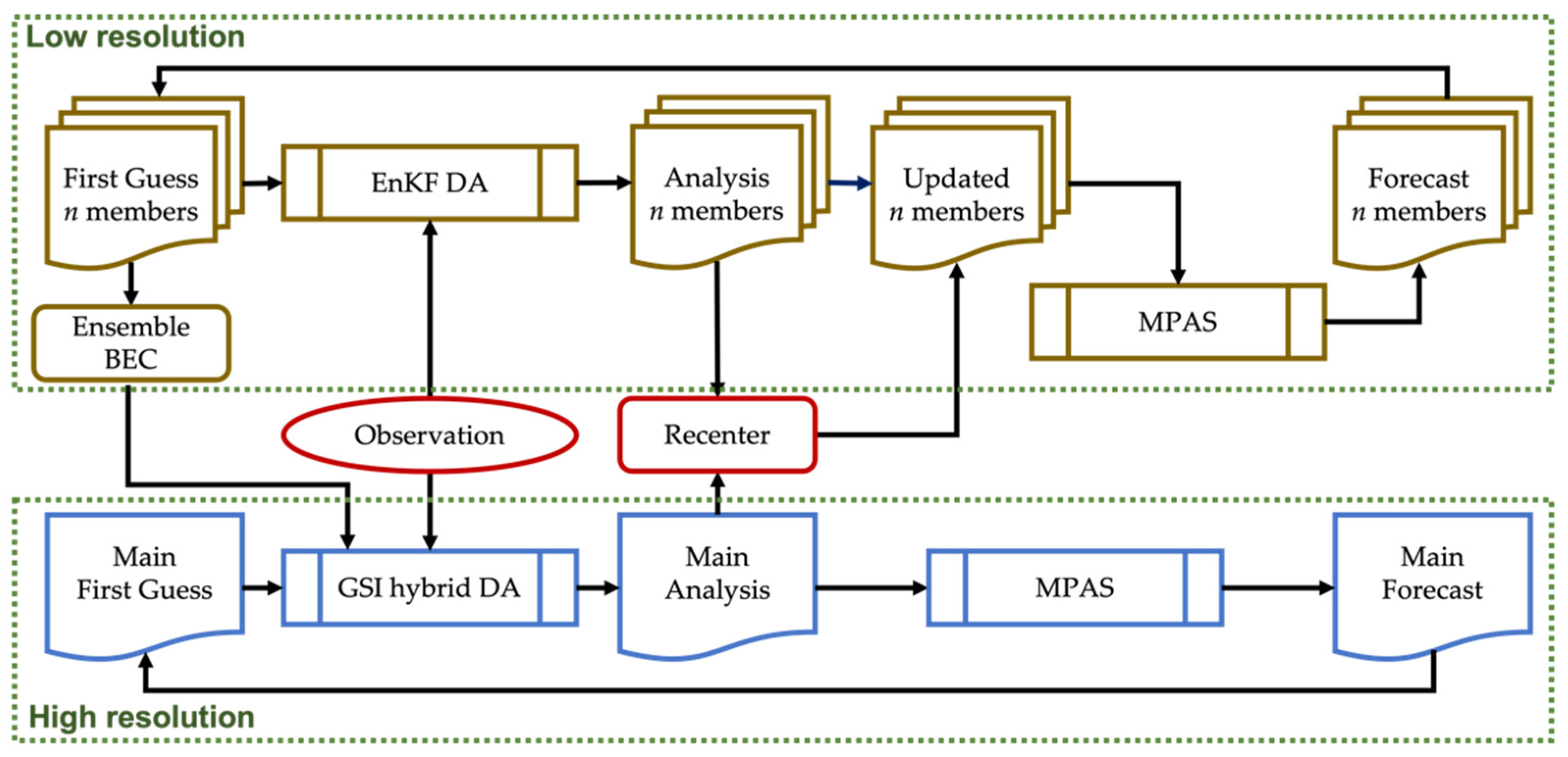
2.1. The Numerical Model and Data Assimilation System

This study applies a non-hydrostatic atmospheric model, the MPAS version 5.2 for DA cycling (developed earlier) and version 6.1 for the free (main) forecast. MPAS was jointly developed by the climate modeling group at Los Alamos National Laboratory and the National Center for Atmospheric Research (NCAR) [1]. The global model MPAS has unstructured centroidal Voronoi meshes with C-grid staggering of state variables, allowing variable-resolution grid meshes with enhanced resolution at targeted regions. For the experiments in this study, the physics schemes for the “mesoscale reference” suite are used, which include the new Tiedtke scheme for cumulus convection [33], the WRF Single-Moment 6 (WSM6) for cloud microphysics [34], the Noah land surface model [35], the Yonsei University (YSU) for the planetary boundary layer parameterization [36], and the Rapid Radiative Transfer Model for General Circulation Model (RRTMG) for longwave and shortwave radiation [37].

NCEP developed the GSI DA system, which can assimilate traditional data, satellite data, radar data, and GPS RO data [6,38]. The GSI system was formulated as a hybrid DA system in 2012 (e.g., [39,40]), which combines the advantages of 3DVAR on static/climatological background errors (BEs) and EnKF on flow-dependent BEs. The GSI system has been implemented and operationally executed at CWB. More details about the GSI system can be found in Chen et al. [22]. Ref. [22] conducted cycling DA with the GSI system and global forecast model at the CWB, which was coordinated with the MPAS simulation for free forecasts.

In this study, we followed [22] but carried out the GSI DA system with the MPAS model for both the cycling DA process and the free forecast. This MPAS-GSI system was developed by NCAR but was not previously documented in the peer-reviewed literature. The primary development challenge of the MPAS-GSI system was appropriately handling various grid meshes: MPAS has an unstructured mesh, while GSI can only produce analyses on a Gaussian grid with regular intervals between latitude and longitude points. Accordingly, the MPAS-GSI system involves an interpolation step, where prior (before assimilation) states are interpolated onto a user-specified Gaussian grid, and the analysis increments are computed within GSI on this Gaussian grid. The increments are then interpolated back onto MPAS’s mesh and added to the prior to complete the DA update on MPAS’s native mesh. In addition, variable transforms are applied to convert MPAS’s prognostic variables [1] to those needed by GSI. MPAS-GSI consists of a variational component as well as an ensemble square-root Kalman filter [41] and is capable of assimilating the full set of observations operationally assimilated at NCEP.

In this work, a recentering process to update the ensemble mean for the EnKF ensemble members is adopted. Use of MPAS-GSI in the DA system is different from [22], in which CWB’s global spectral model was used in the DA system.

2.2. RO Operators

The signal of phase excess between GPS and LEO is used to derive the bending angle (α) through Doppler shift under the spherical-symmetry assumption [30]. The refractivity (N) is related to pressure, temperature, and water vapor pressure [42], and is revised in GSI as

$$N=k_1\left(\frac{P_d}{T}\right)Z_d^{-1}+k_2\left(\frac{P_w}{T}\right)Z_w^{-1}+k_3\left(\frac{P_w}{T^2}\right)Z_w^{-1}$$

(1)

where N = (n − 1) × 10⁶ and n is the index of refraction. In (1), $P_d$ and $P_w$ are the pressure of the dry air and water vapor, respectively; T is the absolute temperature; $k_1$, $k_2$, and $k_3$ are the atmospheric refractivity constants of 77.689 K mb⁻¹, 71.2952 K mb⁻¹, and 3.75463 × 10⁵ K² mb⁻¹, respectively, and $Z_d$ and $Z_w$are the compressibility factors [22]. Through the Abel transform, the local bending angle is computed by

$$\alpha \left(a\right)=-2a{{\displaystyle \int }}_a^{\infty }\frac{d\ln n/dx}{{\left(x^2-a^2\right)}^{1/2}}dx$$

(2)

where a is the impact parameter and x = nr is the refractional radius [26,30,43]. In (2), the bending angle is obtained with the local model refractivity using (1), thus called the local bending angle versus the RO bending angle [30]. RO refractivity then is obtained with the RO bending angle through the inverse Abel transform of (2). The observation operator using (1) is called the local refractivity operator for comparison with the RO refractivity. Thus, the local bending angle operator assimilates the RO bending angle that is more upstream of RO refractivity. Through the assimilation with the two operators built in the GSI, the induced increments (changes) for pressure, temperature, and water vapor pressure can be provided.

2.3. The DVI Method

A description of the DVI method developed for MPAS can be found in Huang et al. [13]. The DVI uses the integration of the complete forecast model in cycle runs of one-hour forecasts from the initial time. The vortex in a radius of 600 km of the vortex center is then relocated to the best track position after each cycle to replace the departure vortex before this forecast. The cycling in DVI is stopped when the central sea-level pressure or maximum wind speed of the simulated vortex reaches or exceeds the best track intensity, called P-match or V-match, respectively. The performances of the DVI with both matches on the typhoon track and intensity predictions are investigated for 16 typhoons in 2015–2020 [13]. The DVI application can improve the typhoon track prediction with statistical significance. This study aims to illustrate the impacts of RO data on typhoon prediction with and without the DVI application.

2.4. Settings of the Model Experiments

The flow chart of the DA system constitutes two parts as shown in Figure 1. For the first part of EnKF, MPAS with 120 km cell spacing was used with 36 ensemble members whose perturbations are created by RANDOMCV, i.e., adopting the module from WRFDA (see [44,45]). The NCEP GFS data are used as the background field in the experiments. To update these EnKF prior ensembles within the MPAS-GSI EnSRF, the 120 km MPAS fields were interpolated to a Gaussian T-106 grid (approximately 125 km horizontal grid spacing). Compared to the one-way system developed in Chen et al. [22] that uses the CWB global spectral model in DA but applies MPAS for the main forecast, the DA system in this study may be called a two-way system since the same forecast model, MPAS, is used in both DA and the main forecast. The background error covariances (BECs) of EnKF are generated by the 36 members at a 6 h forecast for each DA cycle. The 12 and 24 h forecasts in one month of July 2016 by MPAS with 60-15 km resolution were used to derive the static background error covariance using the NMC method [22]. In the second part, hybrid-3DVAR is used with the resolution of MPAS 60-15 km (or 60-15-3 km for higher resolution) with the weighted BECs to update the analysis at each cycle. The 6 h forecast of MPAS is then conducted with the updated analysis for the next DA cycle.

For the hybrid DA system in this study, combined BECs are used by weighting BECs with 75% (flow-dependent) from EnKF and 25% (static/climatological) from 3DVAR, respectively [22,46,47]. The choice of BECs is based on the operational forecast of the global model at CWB that suggests a combination of less static and more flow-dependent BECs. The optimization of BECs for MPAS-GSI was not pursued in this study and it may be sub-optimal compared to the use of full flow-dependent BECs (e.g., Feng and Wang [48]). After DA at each cycle, recentering is performed with the hybrid analysis to replace the ensemble mean and update the ensembles with their perturbations in order to maintain a better stability of split assimilation by the two parts. The homogeneous isotropic horizontal and vertical ensemble localization scale (km) are set to 800 km and 0.8 in lnp unit, respectively. There are two outer loops applied for the GSI-hybrid system, in which 100 and 150 iterations are used in the inner loop. The RO observation errors for both RO operators use the defaults of GSI [22]. The total DA time window with 6 h cycles is two days, from 0000 UTC 2 July 2016 to 0000 UTC 4 July, for the experiments conducted in this study.

The DVI then can be applied to the analysis after the final DA cycle prior to free forecasts. The numerical experiments conducted in this study are listed in

Table 1. Numerical experiments for Typhoon Nepartak (2016). For the experiments, GTS includes the conventional radiosonde soundings (RS), while BND and REF also apply RO bending angle and refractivity soundings, respectively, in addition to the data used in GTS. Note that GTS, BND, and REF used the other observations (OA) (including satellite radiances of AMSU-A and AIRS) routinely available from the CWB. NoDA is the experiment without performing DA (thus, no observations are used).

CASE	Observation	DVI	Resolution (km)
NoDA GTS REF BND	X RS+OA RS+OA+RO RS+OA+RO	X X X X	60-15 60-15 60-15 60-15
GTS_RP GTS_RV REF_RP REF_RV BND_RP BND_RV	RS+OA RS+OA RS+OA+RO RS+OA+RO RS+OA+RO RS+OA+RO	P-match V-match P-match V-match P-match V-match	60-15 60-15 60-15 60-15 60-15 60-15
BND_H BND_RPH BND_RVH	RS+OA+RO RS+OA+RO RS+OA+RO	X P-match V-match	60-15-3 60-15-3 60-15-3

. All the experiments are conducted for 5-day forecasts from 0000 UTC 4 July 2016 to 0000 UTC 9 July 2016. The experiment GTS at 60-15 km resolution assimilates conventional soundings together with all other non-conventional data including satellite radiances (AMSU-A, AIRS, and IASI). The conventional data include GTS soundings, aircraft, satellite-tracked winds, surface pressure observations, ships, and buoys used operationally at CWB. NoDA is the experiment that uses the NCEP FNL as the initial guess (without any data assimilation) and may be used to provide a reference guide for the impact of the hybrid DA. BND and REF are the same as GTS but assimilate additional RO bending angle and refractivity, respectively, while BND_RP and BND_RV are the same as BND but are combined with the DVI with P-match and V-match, respectively. It is similar for REF_RP and REF_RV, as well as GTS_RP and GTS_RV. For comparison with the results at 60-15 km resolution, the higher-resolution experiments with the 60-15-3 km grid mesh are also conducted for BND with and without the DVI. The grid mesh of 60-15-3 km can be seen in Chen et al. ([22], Figure 3). For these sensitivity tests, the resolution of 60-15-3 km is also applied in the cycled DA and the MPAS main forecast of 5 days. Note that in each DA cycle, the high-resolution of 60-15 or 60-15-3 km is used in the 6 h forecast after 3DVAR analysis, while GSI uses the analysis at the coarser resolution of 120 km for 6 h integration of each member.

As the 60-15-3 km resolution is used for the sensitivity tests, the scale-aware problem may be associated with application of cumulus parameterization. When the horizontal resolution is highly increased at some regions, specific cumulus parameterization may not be scale-aware without any adjustment causing the misrepresentation of convection. This would not be critical for the previous simulations with the coarser 60-15 km resolution; even the new Tiedtke scheme applied in the current “mesoscale reference physics suites” of MPAS 5.2 is not a scale-aware scheme. We tested the scale-aware scheme (Grell–Freitas) available in MPAS 5.2. The simulation results with the Grell–Freitas scheme, however, have no particular improvement but with a more southward track deviation at earlier stages compared to that with the new Tiedtke scheme. When more scale-aware cumulus parameterizations are available in MPAS, it is worth conducting further sensitivity tests to illustrate the impacts of the scale-aware convection on the typhoon forecasts.

3. Simulations and Discussion

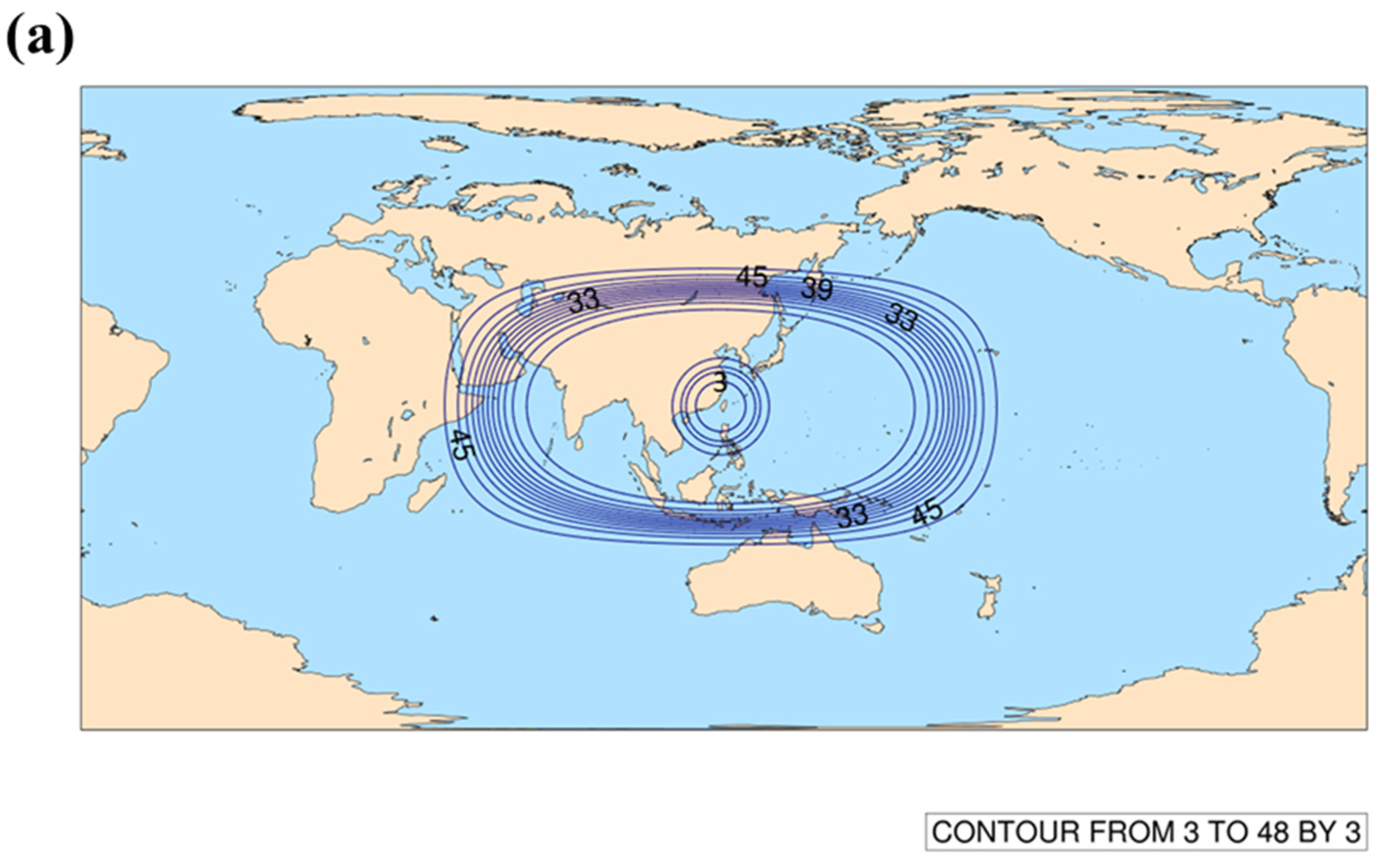
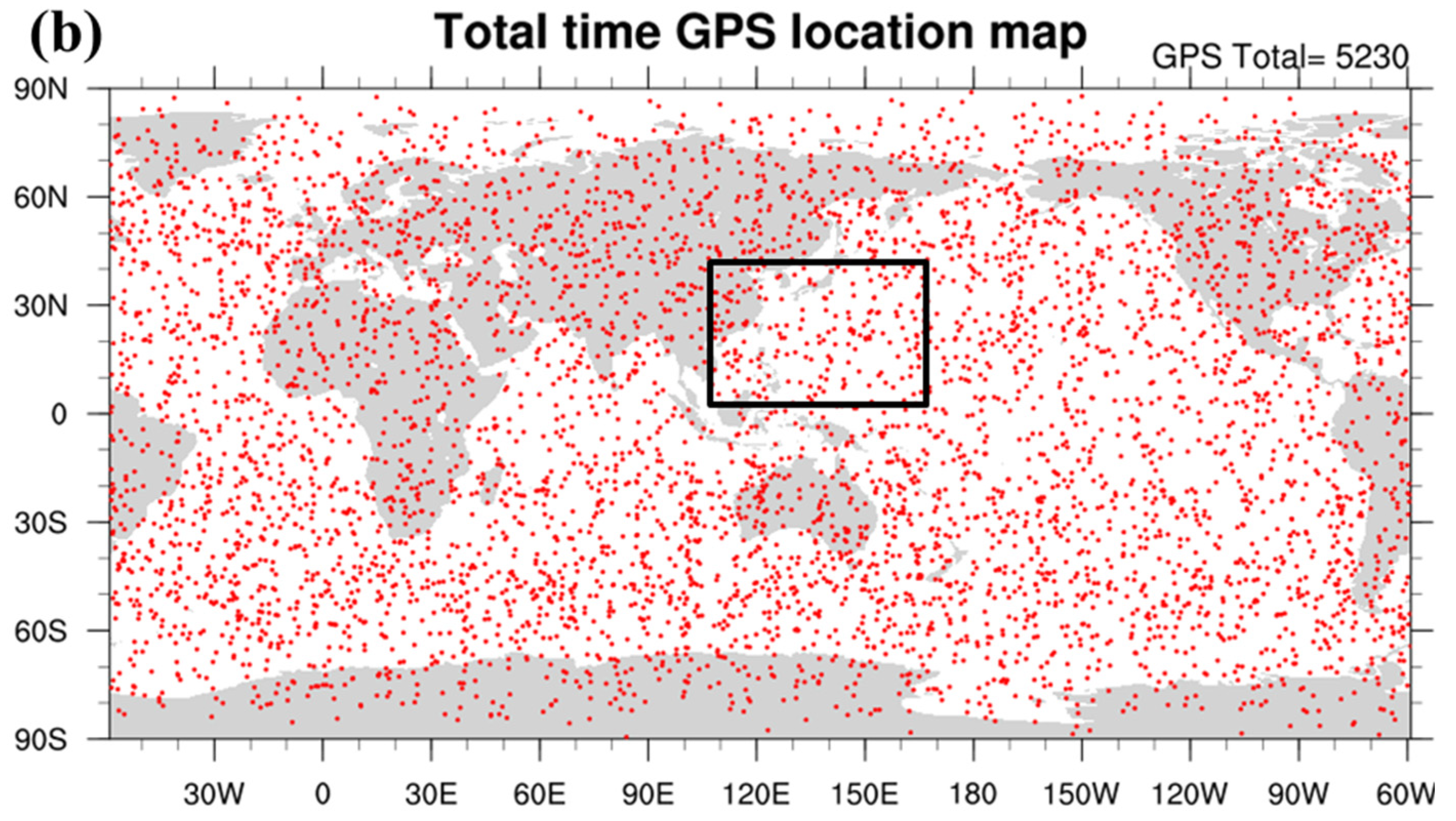
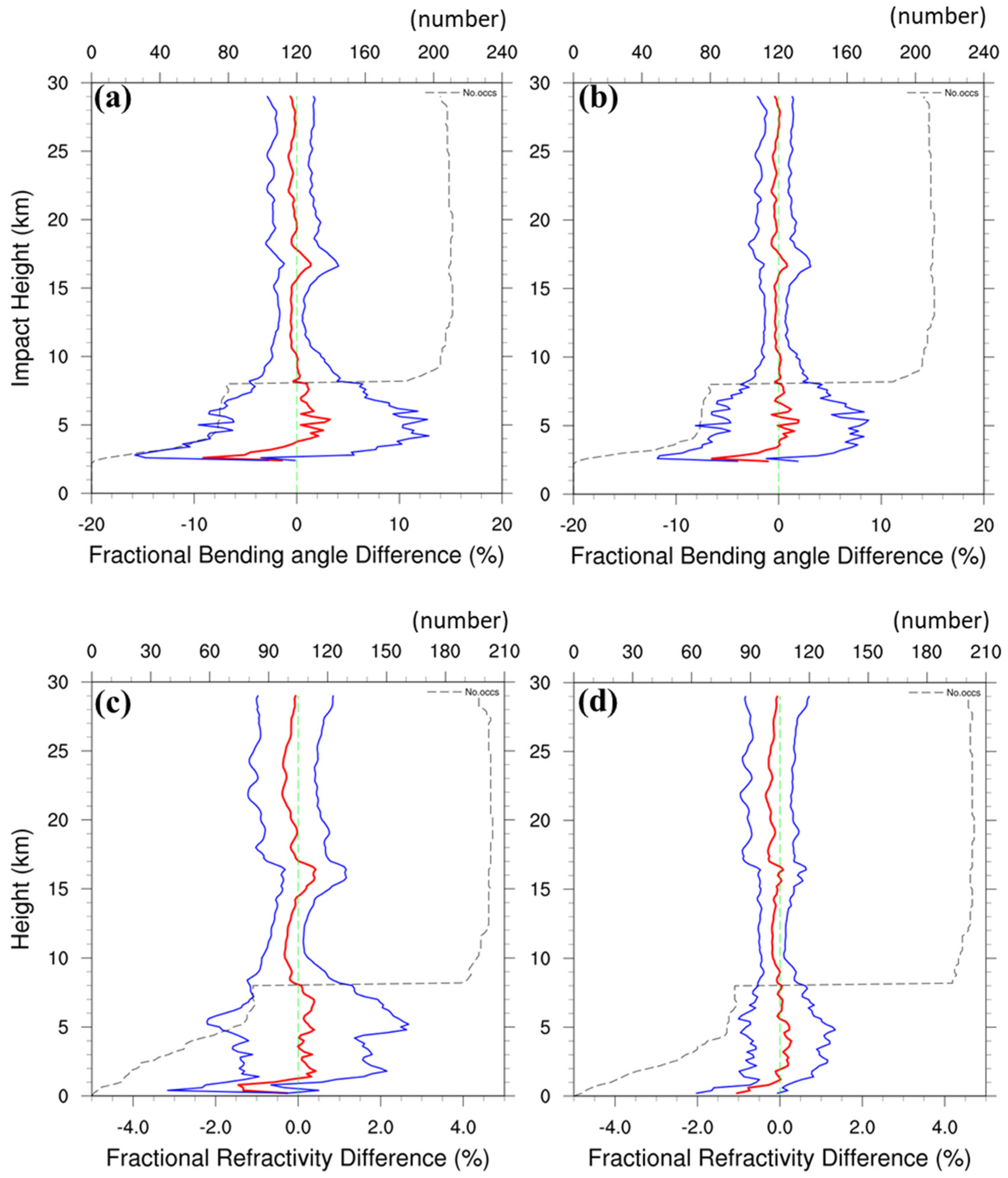
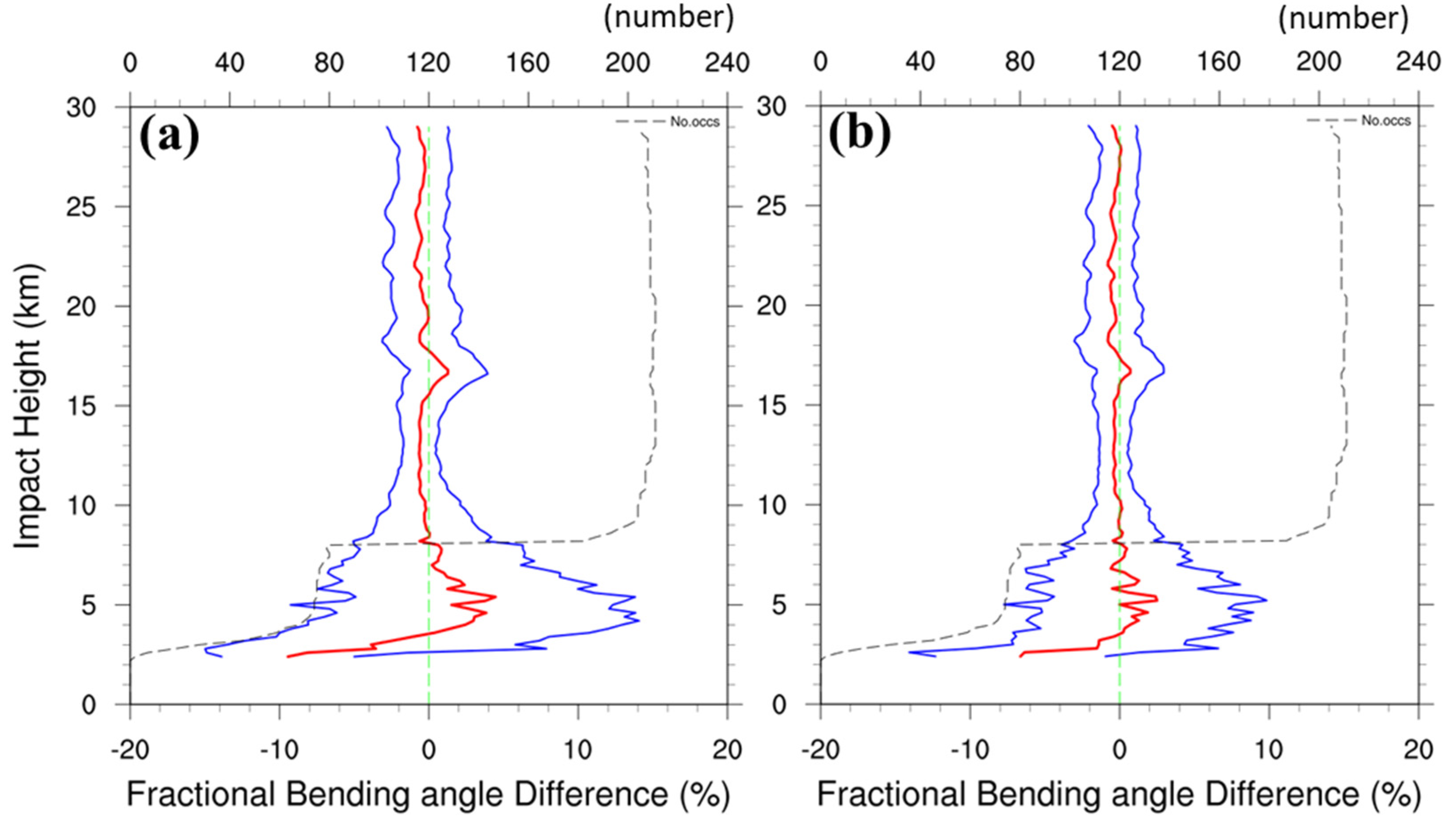
3.1. The RO Data Used in the Assimilation

Figure 2 shows the locations of GPS RO soundings assimilated in the DA period of 0000 UTC 2–4 July 2016. There are a total of 5230 RO soundings in the globe with 211 soundings located in the region of 0–40° N and 110–170° E spanning the typhoon track. This local region was chosen for the verification against the European Centre for Medium-Range Weather Forecasts (ECMWF) analysis shown later. The assimilated RO data that came from FS3/C, Meteorological Operational satellites (MetOp), Gravity Recovery and Climate Experiment (GRACE), X-Band TerraSAR satellite (TerraSAR-X), and TerraSAR-X add-on for Digital Elevation Measurement (TanDEM-X) are irregularly distributed but with quite uniform data density in the global and local regions. A reduced data density can be found in the tropical and polar regions as FS3/C is a constellation of six LEOs at 72° inclination that can provide denser occultation in mid-latitudes.

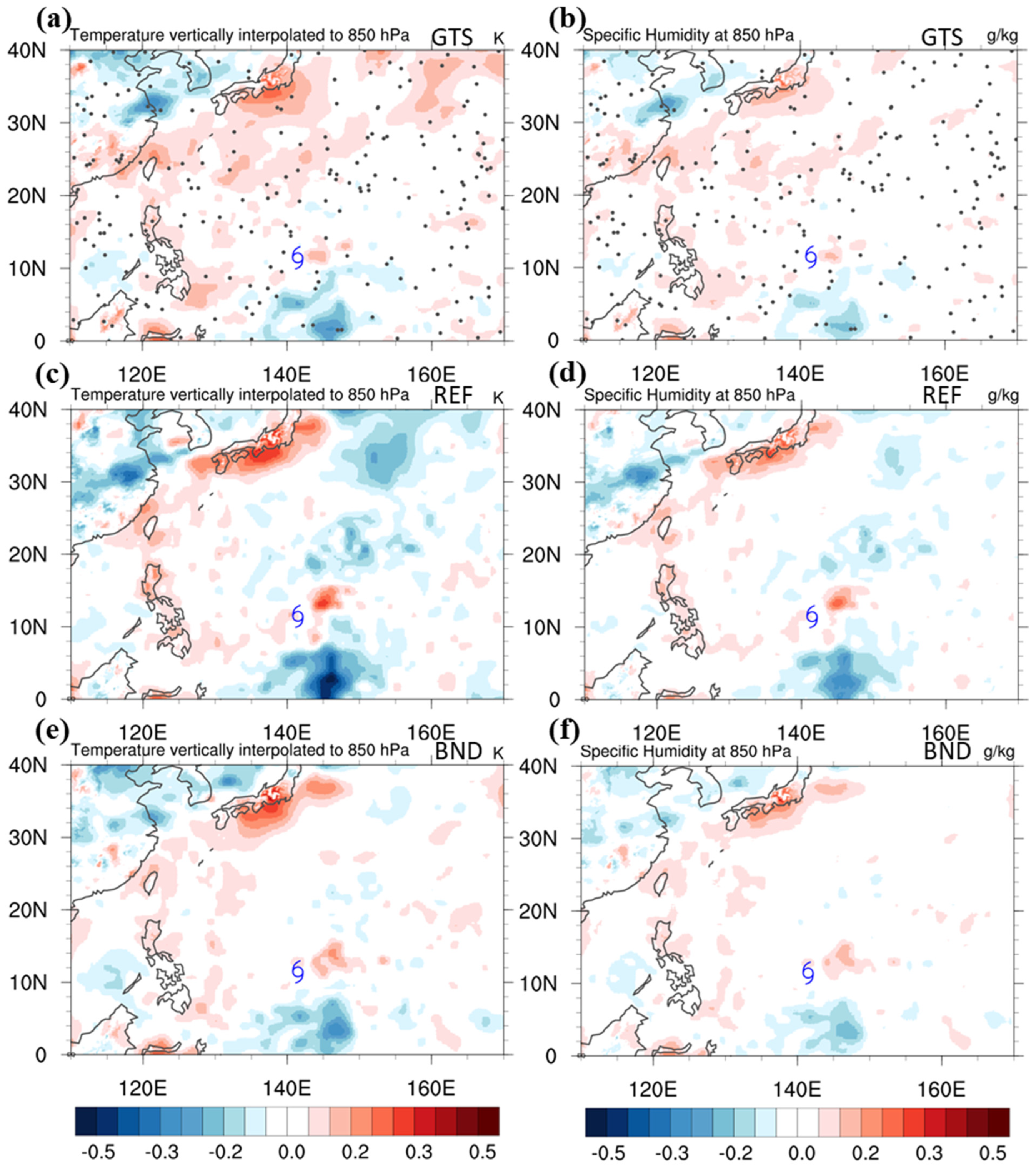
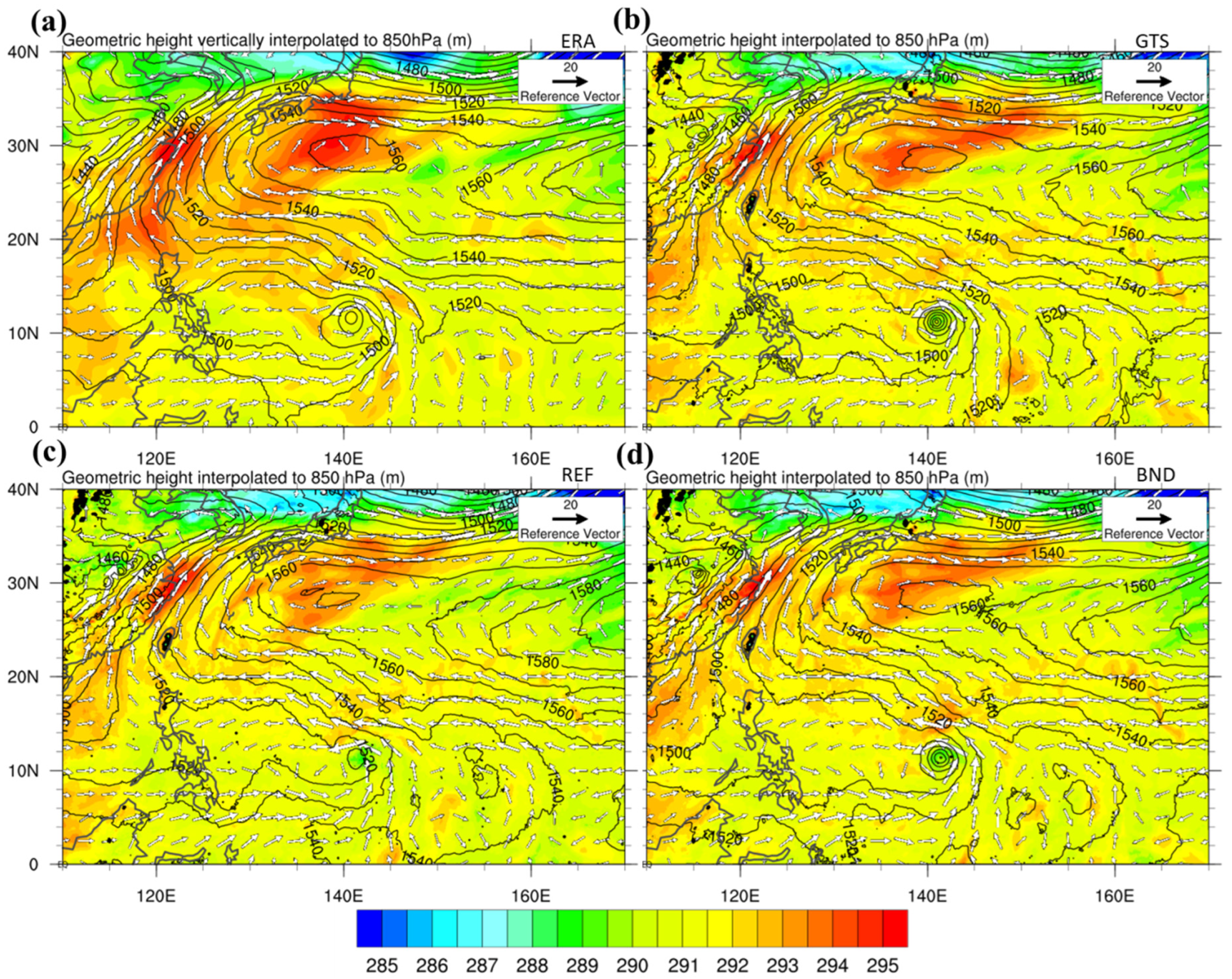
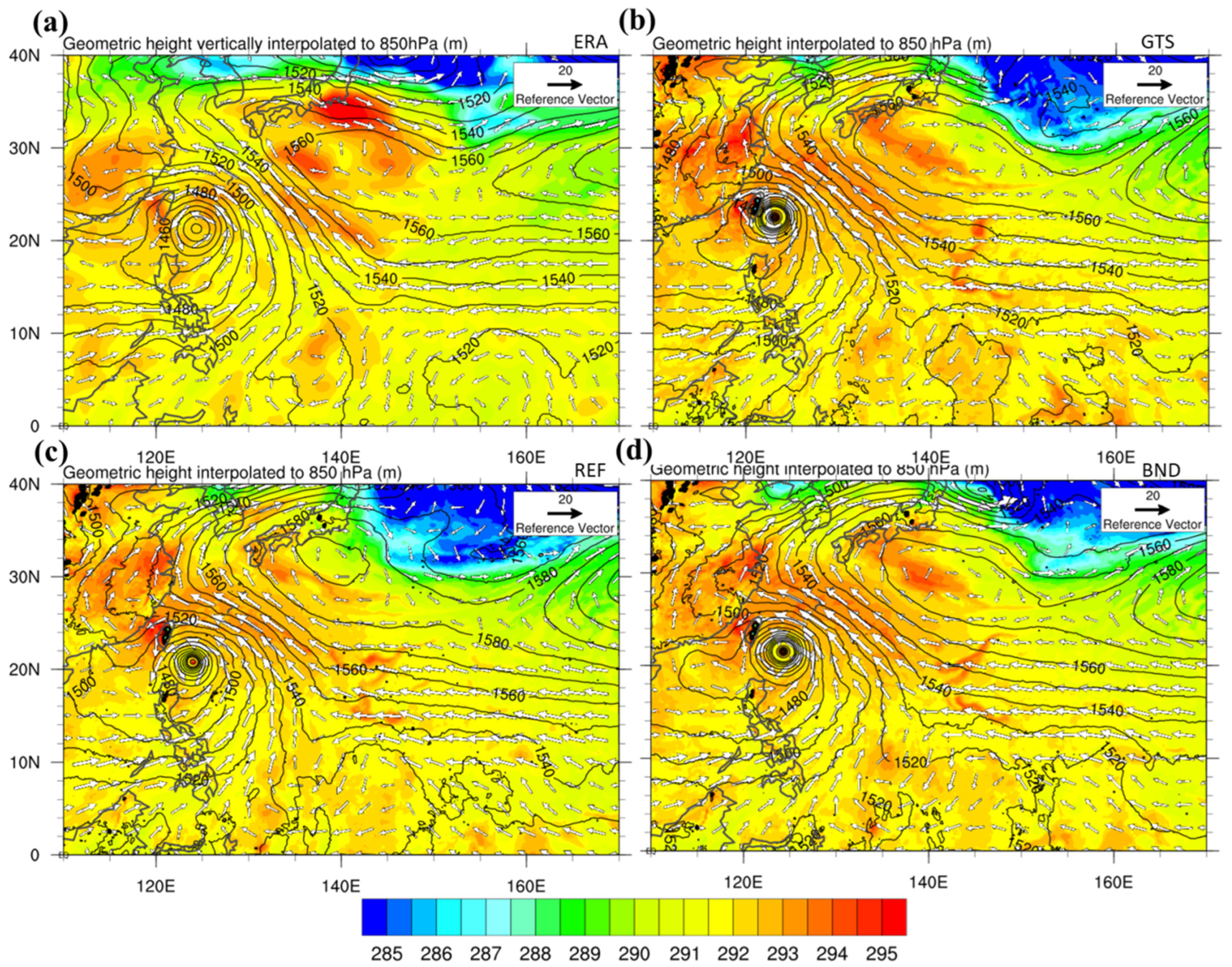
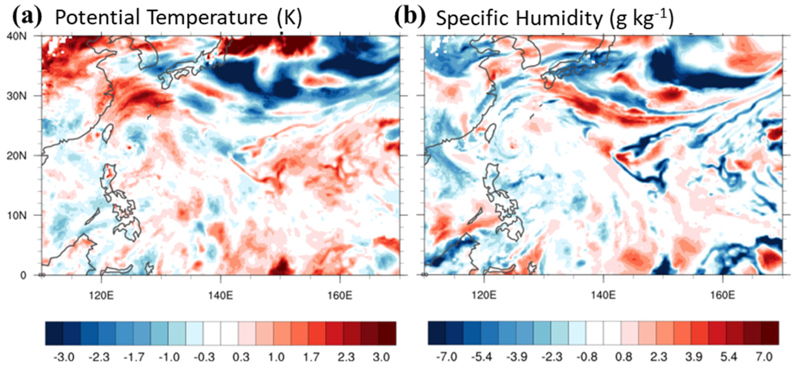
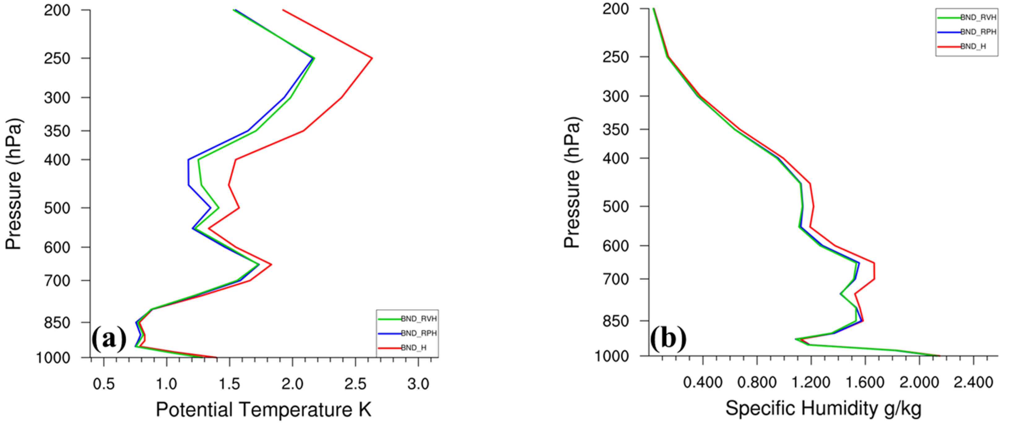
3.2. Initial Analyses after Data Assimilation

The fractional differences and their standard deviations between the observation (O) and the first guess (B) as well as the observation (O) and the analysis (A) averaged during the DA in the local verification region are shown in Figure 3 for REF and BND. The amounts and distributions of the RO profiles assimilated after quality control of GSI are similar for refractivity and bending angle, with about 200 profiles above 10 km impact height and only about 40 profiles near 3 km height during the DA window. At upper levels above 10 km impact height, the magnitudes of both fractional differences and standard deviations for REF and BND are much smaller due to both RO refractivity and bending angle decreasing rapidly with height. The results for BND indicate that the deviation of O from B, i.e., the innovation (O−B), was reduced in O−A with smaller magnitudes in the mean fractional differences (from 3% to 2%) and standard deviations (about a maximum reduction of 4% from 13% to 9%) below 5 km height (Figure 3b). Similar reductions are also found for REF but with a slightly larger reduction extending to the upper level near 10 km height. With the extra RO data (bending angle and refractivity), the hybrid assimilation showed an efficient reduction on the analysis difference after the DA period. The fractional differences and their standard deviations of bending angle from FS3/C are similar to that shown in Lien et al. [49] from FS7/C2.

Figure 4 shows the horizontal distributions of temperature and specific humidity increments at 850 hPa averaged during DA. The increments are the differences between the DA analysis and the first guess after each cycling (6 h window) and they are averaged during the DA. Larger positive increments are produced near the location of Typhoon Genesis (145° E, 12° N) and Japan for BND and REF (Figure 4a–d) than GTS (Figure 4e,f). South of the typhoon center, larger negative increments in both temperature and specific humidity are induced for REF than BND, while both are more intense than GTS. It is noted that considerably negative temperature increments and moderately negative specific humidity increments are produced east of Japan above the typhoon region for REF, which is not found for BND. The results indicate that the impacts of additional RO data give further modification on the model temperature and moisture analysis through the hybrid assimilation.

To verify the assimilation results with the RO data, the wind, temperature, and geometric height analyses at 850 hPa at 0000 UTC 4 July 2016 (the end assimilation) are compared with the ECMWF reanalysis (ERA-Interim) [50] in Figure 5. There is a cut-off high extending from the western flank of the subtropical high, where all three experiments gave a colder temperature compared to ERA-Interim. REF provided the weakest intensity of the warm air with the narrowest high core than both GTS and BND, which could be possibly due to the colder and drier increments induced by the RO data assimilation in Figure 4. Near the inner typhoon, there are few differences in the geometric height for the three experiments, which compared well with ERA-Interim. However, the wind and pressure intensities of the typhoon for BND and GTS (Figure 5b,d) are considerably stronger than those for REF (Figure 5c) and are also more intense than the ERA-Interim (Figure 5a). Typhoon intensity may be somewhat under-predicted by the global model assimilation as in the ERA-Interim. Indeed, the CWB best-track maximum wind (shown later) is stronger than that for both BND and GTS. The overall wind and geometric height distributions in the environment surrounding the typhoon are consistent with the ERA-Interim for the three experiments, except for the region of the cut-off high.

All the experiments are conducted with the resolution of 60-15 km and initialized 5-day MPAS forecasts at 0000 UTC 4 July 2016. Figure 6 shows the track and intensity of the forecasted typhoon for GTS, REF, and BND, compared to the CWB best track data. The results without any DA (NoDA) are also included for comparison. The forecasted tracks for all the experiments are in good agreement with the best track before 0000 UTC 7 July, but closer to the best track in the earlier three days obviously for the DA experiments (GTS, BND, and REF) compared to NoDA. It is noticed that that NoDA gives a much slower translation when moving closer to the terrain with the largest northward track deflection after 3 days (Figure 6a). The track for REF is associated with a generally southward deviation after 24 h, compared to BND and GTS. However, the track errors for REF are comparable to those for BND in the first three days and indeed are smaller afterward due to the fact that the BND track has deviated northward afterwards (Figure 6b). The typhoon intensities for all DA experiments are weaker than the best track intensity, especially near and after landfall in Taiwan; however, only the intensity for NoDA is stronger than the best track intensity at the initial time and on the first day (Figure 6c). Consequently, NoDA still maintains a stronger typhoon more comparable to the best track intensity than the other experiments throughout the forecast. It is apparent that the typhoon intensity for BND is much stronger than that for REF, as already shown earlier. Although BND and GTS have further under-predicted typhoon intensities than NoDA; their intensification rates are similar in the first three days. Again, REF obtains the weakest typhoon intensity in the first three days, which is consistent with Figure 5. In this study, we focused on the track and intensity evolution of the typhoon before landfall as the topographic effect of Taiwan terrain will greatly complicate the responses of the impinging typhoon near and after landfall. The typhoon intensity may correlate to the accumulated mid–lower tropospheric increments during the DA, as discussed in Chen et al. [24]. The impacts of RO data appear to be substantially larger for typhoon track forecasts than intensity forecasts [20,22,23] as the RO observations can only directly retrieve the thermodynamic information from (1). Though DA, the wind structure and intensity of a TC vortex is only slightly adjusted by RO data assimilation. Observations that may provide or retrieve the wind information will be helpful for TC intensity forecasts, which constitutes the reason why the DVI is combined with RO data assimilation to spin up the TC in this study.

These track forecasts for NoDA, GTS, REF, and BND compare well with those in Chen et al. ([22], Figure 10) using the one-way system, except the BND track is slightly better on day 3 but indeed worse on day 5. The intensity forecasts for GTS and BND are similar for both systems, but the two-way system produces a slower deepening on day 1 but a faster intensification on day 3. As shown in Figure 6, the simulated typhoon intensity for REF is much weaker than that for GTS and BND in days 2 and 3 using the two-way system, while it is similar in these three experiments using the one-way system. These differences might be partially attributed to the fact that the hybrid DA analysis is influenced by the updated background covariance computed by the ensemble forecasts using either MPAS or CWB GFS. Note that due to computational loading, the coarser resolution is applied for the ensemble members in this study. The background covariance structure may be further improved with the same higher resolution to improve the DA analysis [48].

For understanding the track responses for GTS, REF, and BND, Figure 7 shows the forecasted geometric height, temperature, and wind at 850 hPa at 0000 UTC 7 July 2016 (after 3-day forecasts) when their tracks begin to deviate greatly as shown in Figure 6a. The temperature presents a warmer intensity in the vicinity of the typhoon for the three experiments compared to the ERA-Interim temperature. The predicted typhoon for REF (Figure 7c) becomes much stronger at the end of the assimilation, but is still weaker than those for GTS and BND (Figure 7b,d), all more intense and closer to the best track than the ERA-Interim as also shown in Figure 6c. However, the environmental field including the western flank of the extended high for BND and GTS has an alignment more northward than that for REF, in association with more northward wind components mainly east of the inner typhoon. The extended high is also stronger in REF and produces more westward wind components near the north of the inner typhoon. Such combined effects may facilitate a more westward and less northward movement of the typhoon in REF, as shown previously by the actual typhoon movement.

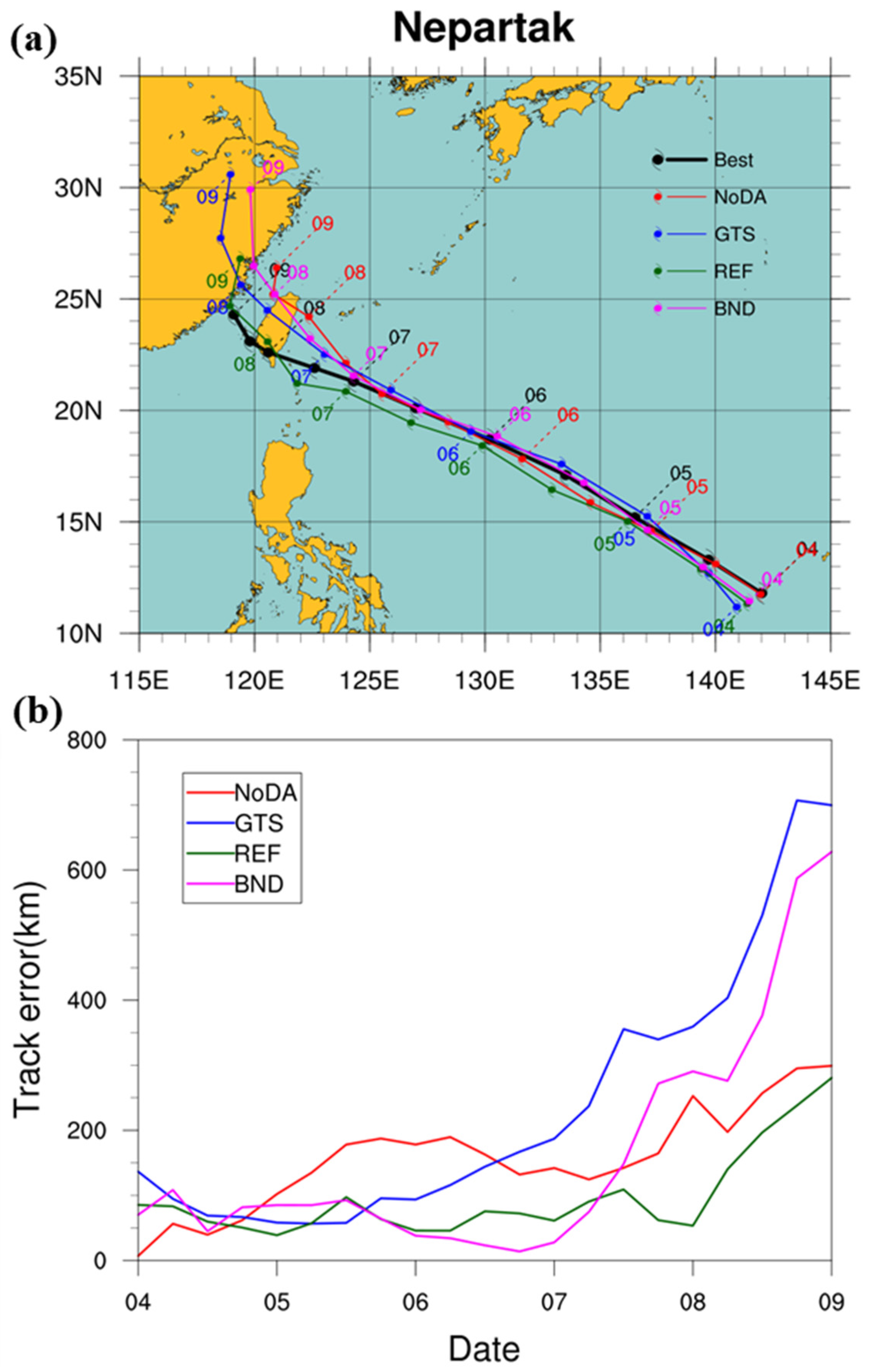
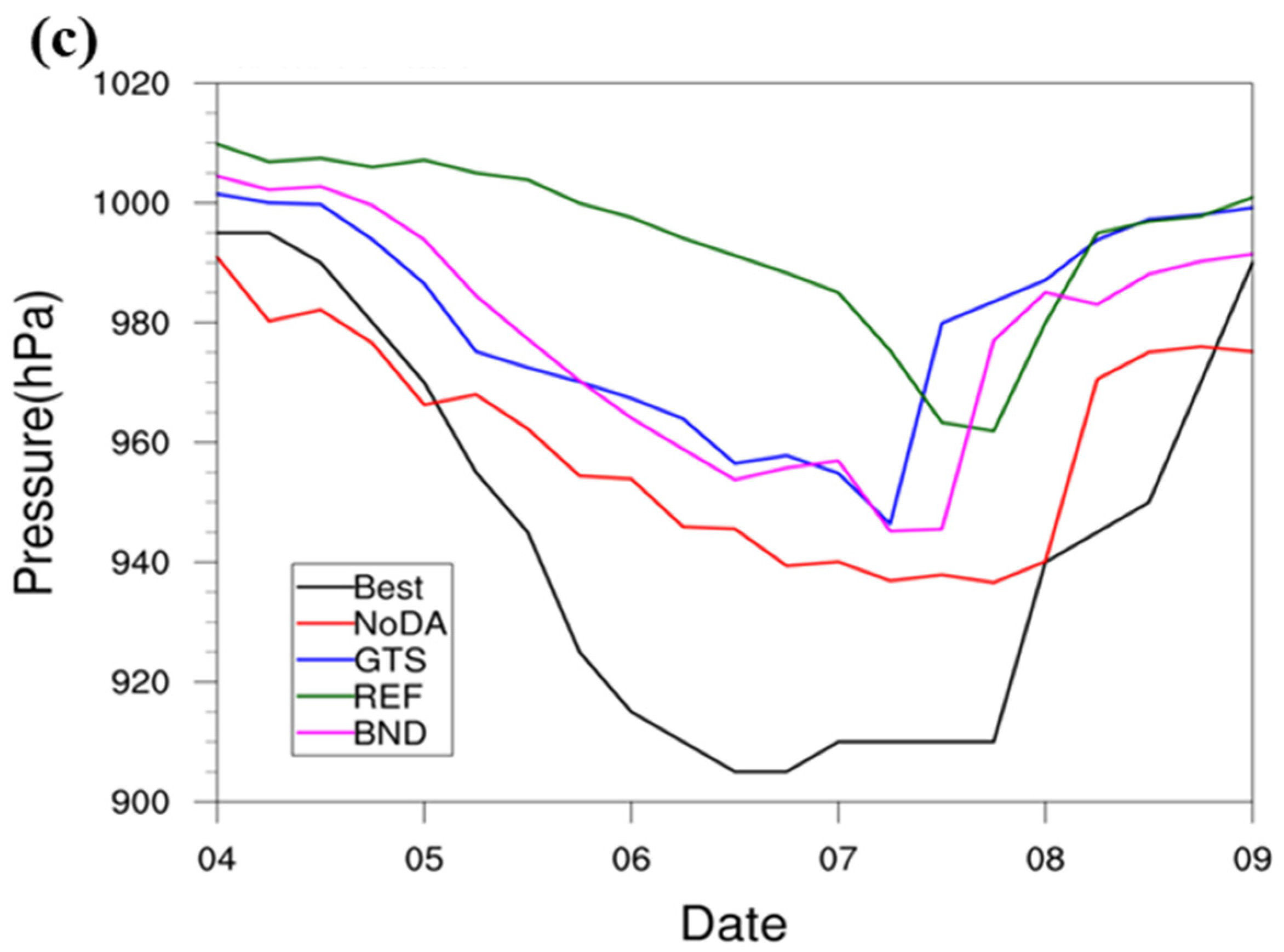
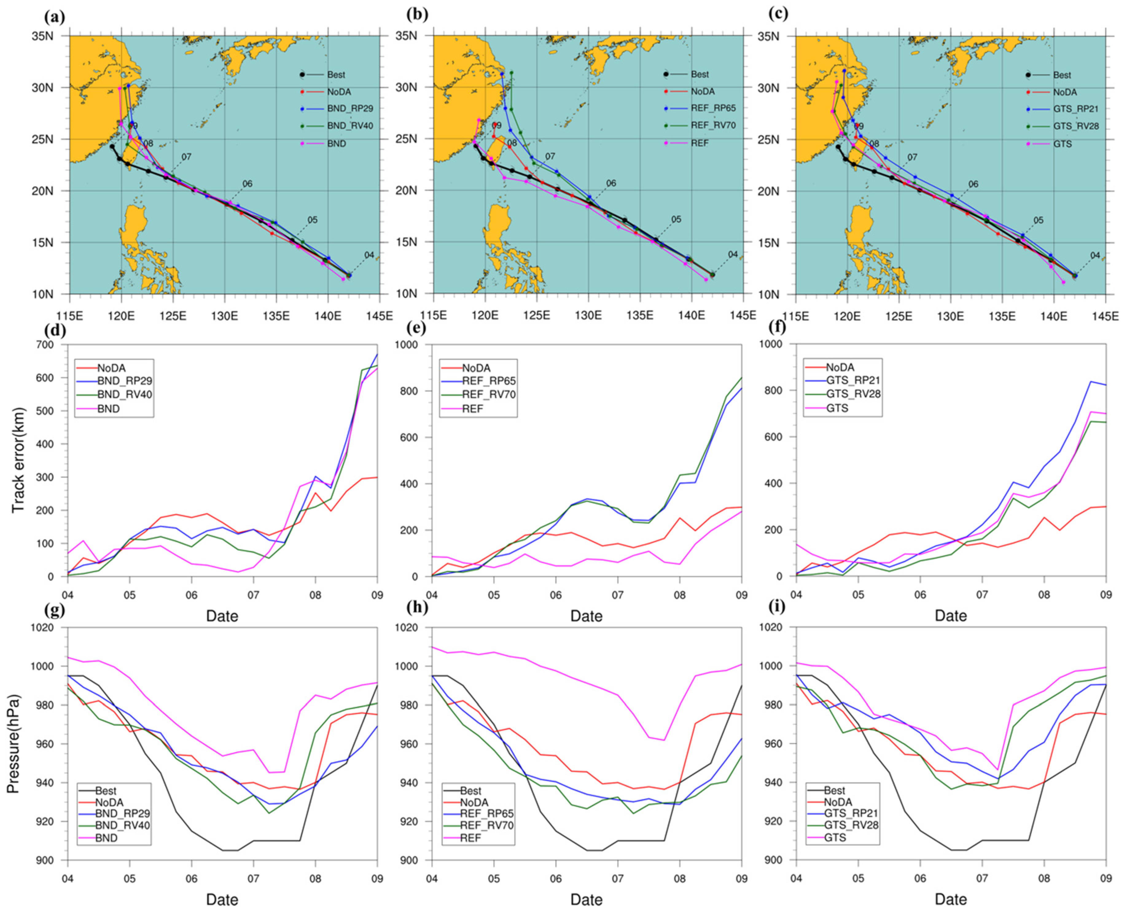
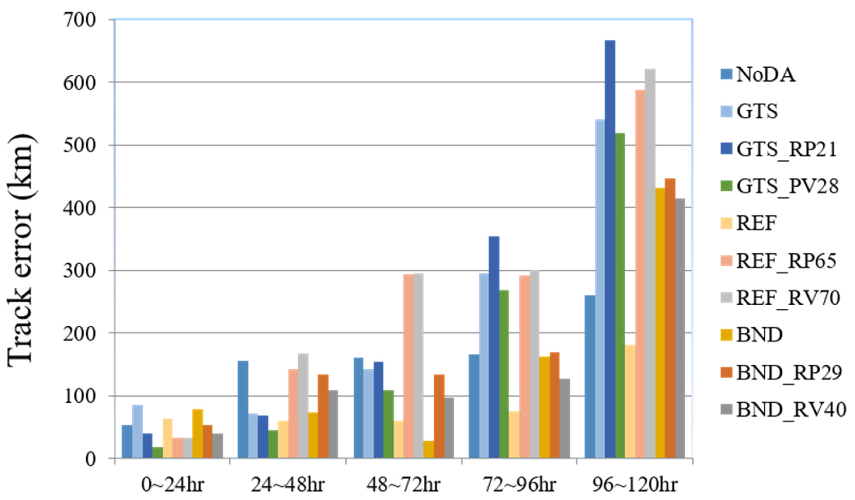
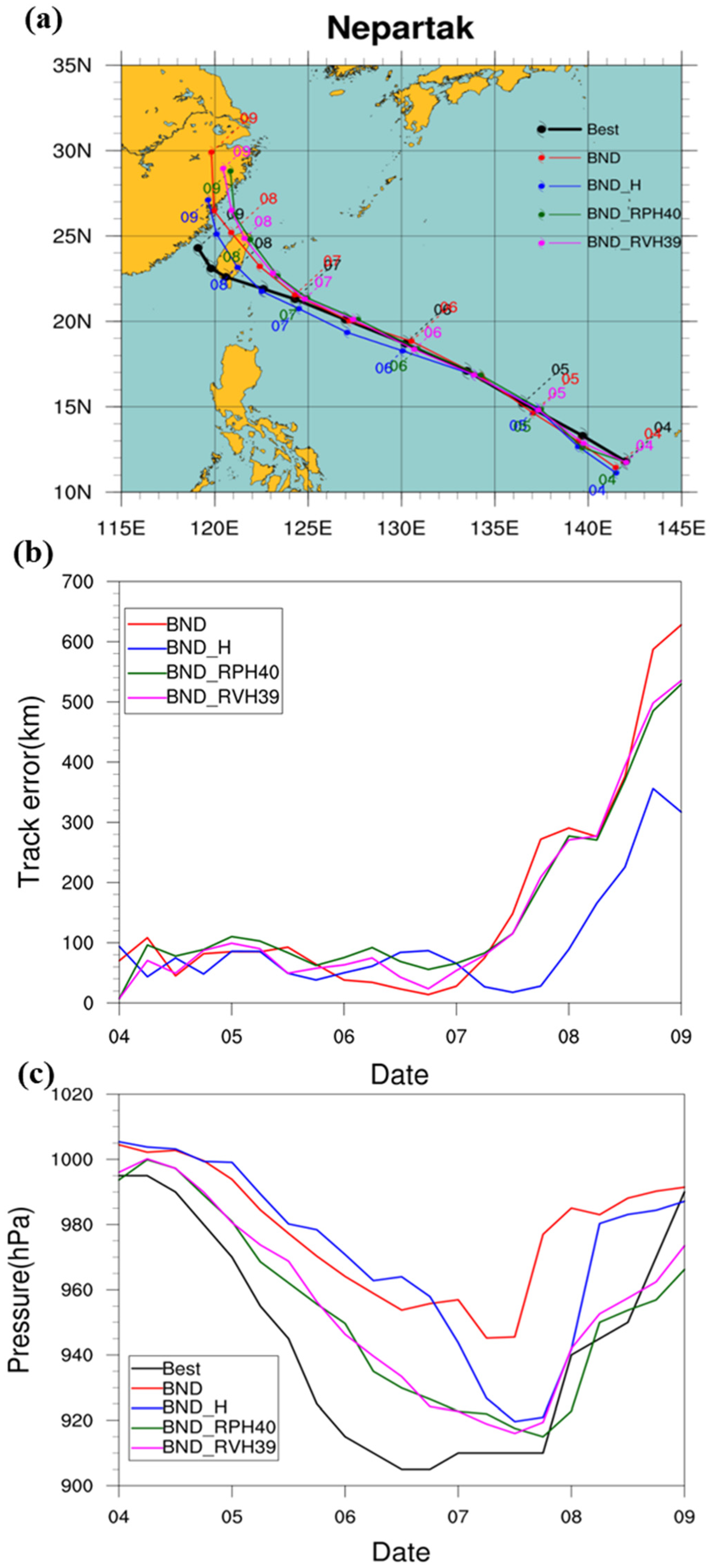
3.3. Forecasted Results with DVI

All DA experiments with the DVI were conducted for 5-day forecasts, where either P-match or V-match was chosen for the cycle runs using the analysis at the end of the cycling assimilation. Figure 8 shows the track and intensity for all DVI experiments, which are compared to the CWB best track. Regardless of the selected match for GTS, REF, and BND, the typhoon intensities for the DVI experiments are in better agreement with the best track intensity than the experiments without the DVI (Figure 8g–i). Note that the required cycle runs for P-match are lower than that for V-match. In general, the forecasted tracks are not significantly changed for all the experiments with and without the DVI for GTS, REF, and BND (Figure 8a–c). However, the DVI appears to slightly improve the track prediction for REF and BND, and eliminate the southward deviation for REF. For BND_RV40, REF_RV70, and GTS_RV28, their track errors at 120 h are quite close, nearly 300 km. Here, the number following the experiment (see Table 1) indicates the required cycle runs associated with the match in the DVI. The track forecast with the DVI is still slightly worse for REF and BND, but the noted underprediction in intensity was significantly improved. Apparently, the underestimate of the RO data assimilation on the best track intensity due to the scarcity of RO data in the inner typhoon was largely overcome by the DVI.

The daily averaged forecast track errors for all the experiments with and without DVI are summarized in Figure 9. The track errors in all the experiments with the DVI are reduced in the first day, compared to those in the experiments without the DVI. However, the errors are increased for the DVI experiments in days 2 and 3 and remain similar in days 4 and 5, except for REF as shown in Figure 8. These results imply that the DVI can improve the intensity forecast but has no large positive impact on the track forecast. At later stages, the DVI tends to have more positive effects on RO assimilation for BND than REF. The smallest track errors at days 4 and 5 for REF without the DVI are benefited by its more consistent movement but at the cost of the largest underprediction on typhoon intensity.

To understand the differences in the forecasts after the DVI, their forecasted geometric height, temperature, and wind vector at 850 hPa are shown in Figure 10. With the DVI, the inner typhoon core was significantly enhanced at 0000 UTC 4 July 2016 for BND_RP (Figure 10a) as compared to that without the DVI for BND (Figure 5d). Note that the relocation of the vortex center also shifted the analysis vortex to the best track position that is somewhat east of the typhoon center in BND. Figure 11 shows the differences between the forecasted temperature and specific humidity at 850 hPa at 72 h for BND_RV. At 72 h, the forecasted flow fields for BND_RP are very similar to BND_RV. Indeed, both fields are also similar to that for BND, except for the typhoon circulation (figures not shown). Consequently, all three experimental results exhibit similar differences from the ERA-Interim, with warmer air to the north and east of the outer typhoon and more moistening mainly in the inner typhoon in the lower troposphere. The temperature warming to the north of the typhoon center might be a factor of the northward track deviation after 72 h for the three experiments.

3.4. Higher-Resolution Forecast Results with the DVI

The above experiments were conducted using the resolution of 60-15 km for MPAS forecasts. For the sensitivity tests on model resolution, the higher resolution of 60-15-3 km is used for MPAS forecasts in both the hybrid DA and free forecasts. The same static B is utilized at the DA for the higher-resolution experiments because DA still uses the same resolution settings. Since the BND experiment exhibits better performance on track forecast, we focused on the BND experiment for the investigation with higher resolution.

At the end of DA, the mean differences and standard deviations for O−B and O−A during DA with RO data are shown in Figure 12; the mean differences are the average of the differences over the verification area as shown in Figure 3a. The vertical variations in O−B (Figure 12a) and O−A (Figure 12b) are similar in the experiment BND_H (similar to BND but with the resolution of 60-15-3 km), while the differences and standard deviations of the BND are relatively smaller with about half reduction in the troposphere compared to those of the BND_H. Compared to the DA results with 60-15 km resolution in Figure 3, use of the 60-15-3 km resolution appears to further reduce the magnitudes of O−A from the larger mean differences and standard deviations (Figure 12a vs. Figure 3a) but maintain similar variations and magnitudes. The horizontal distributions of the induced temperature and specific humidity increments at 850 hPa after the DA for BND and BND_H are quite similar (figures not shown).

Figure 13 shows the track and intensity forecast for BND and the higher-resolution experiments, BND_H, BND_RPH, and BND_RVH. Note that the DVI in BND_H, BND_RPH, and BND_RVH reaches the best track pressure and wind intensity after 40 and 39 cycles. The track for BND_H agrees best with the best track (Figure 13a), showing a slightly southward deviation after 48 h but a less northward deviation after 84 h than the other experiments. Indeed, the track errors for BND_H are less than 100 km at 96 h and only about 300 km at 120 h. For BND_RPH and BND_RVH, the track errors are close to BND_H in the first three days, but with a much larger growth rate afterward (Figure 13b). Use of the higher resolution for BND resulted in an improved track forecast in BND_H, which, however, is not further improved by the complementary DVI at the end of DA for enhancing the inner typhoon. Comparing the track and intensity forecasts for BND_H, the two-way system produces a faster and more consistent deepening rate in days 2–4 than using the one-way system in Chen et al. ([22], Figure 18). The two-way system also gives the smallest track error (about 50 km on average) in day 3 as seen in Figure 13b. Despite this noted improvement in track and intensity forecasts in day 3 for BND_H, both the systems perform about equally for this typhoon.

The intensity forecasts with the higher resolution also exhibit similar benefits from the DVI as shown in Figure 13c where both BND_RPH and BND_RVH obtain more deepening in the first four days and a consistent decaying in the last day, in better agreement with the best track data than BND and BND_H (without the DVI). It can be attributed to the initial spin up of the typhoon vortex core by a deepening of about 10 hPa for both DVI experiments. It is noted that BND_H obtained a much faster deepening roughly after day 3 before landfall in Taiwan than BND. With a more southward position following the best track, the typhoon of BND_H before landfall may encounter weaker mountain blocking than that with a northward deviated track of BND. Compared to the best track data, all the experiments showed weaker vortices but with rather consistent tracks before moving closer to the terrain. Given the more consistent track and intensity forecasts before landfall, the forecast of accumulated rainfall over Taiwan is also improved for both DVI experiments (figures not shown).

Figure 14 shows the differences in temperature and specific humidity at 850 hPa for the BND_RVH experiment from the ERA-Interim. The differences are similar for both BND_RPH and BND_RVH (not shown). Compared to Figure 11 for BND_RP, the temperature differences are reduced, especially to the north of the outer typhoon and east of the inner typhoon as well as far southeast of the typhoon. For moisture, the major reduction is found in the inner typhoon where the wetter condition in BND_RV over the vortex core was largely decreased in BND_RVH.

The averaged RMSEs of temperature and specific humidity verified against the ERA-Interim over the verification area at 0000 UTC 7 July 2016 for BND_H, BND_RVH, and BND_RPH are shown in Figure 15. Compared to BND_H, the RMSEs of temperature and moisture were reduced throughout the troposphere, especially above 700 hPa, for both DVI experiments. A greater reduction at the 72 h forecast is obtained in the mid–upper troposphere, which indicates that the DVI not only enhances the initial inner typhoon but also helps produce a more persistent and stronger development as seen in Figure 13c. The relative impacts for V-match and P-match are mixed in both temperature and moisture differences. It appears that P-match gives a better temperature forecast above 700 hPa but slightly degraded moisture forecast below 500 hPa. Which match is preferred for typhoon forecasts remains inconclusive.

3.5. PV Budget Analysis

For understanding the track deflection, potential vorticity (PV) tendency budget is useful for providing an explanation for the typhoon track responses to different physical processes involved in the PV tendency equation as already illustrated in Chen et al. [22]. The typhoon track at 0000 UTC 7 July for BND_H is more southward than that for BND as shown in Figure 13a. Figure 16 shows the wavenumber-one (WN-1) PV tendency budget averaged at 1–8 km height at 0000 UTC 7 July 2016 for BND and BND_H. For BND, the west–northwestward translation of the typhoon indicated by the net PV budget (Figure 16a) essentially follows the translation velocity induced by horizontal PV advection (Figure 16b) that is slightly offset by differential diabatic heating (Figure 16c). For BND_H, the induced typhoon movement is faster and becomes northwestward and is closely related to the net PV budget (Figure 16d) and horizontal PV advection (Figure 16e), while the differential diabatic heating is much weaker (Figure 16f). The induced typhoon translations for both experiments are in agreement with the WN-1 flow in Figure 16 and the actual typhoon movement shown in Figure 13. Thus, the more northward movement of the typhoon after 0000 UTC 7 July for BND_H is primarily controlled by the horizontal PV advection as a consequence of flow steering.

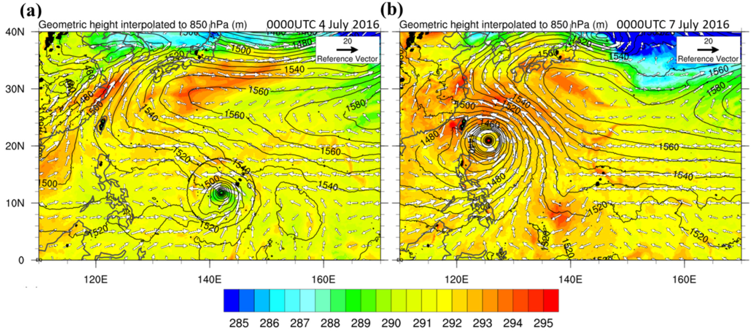
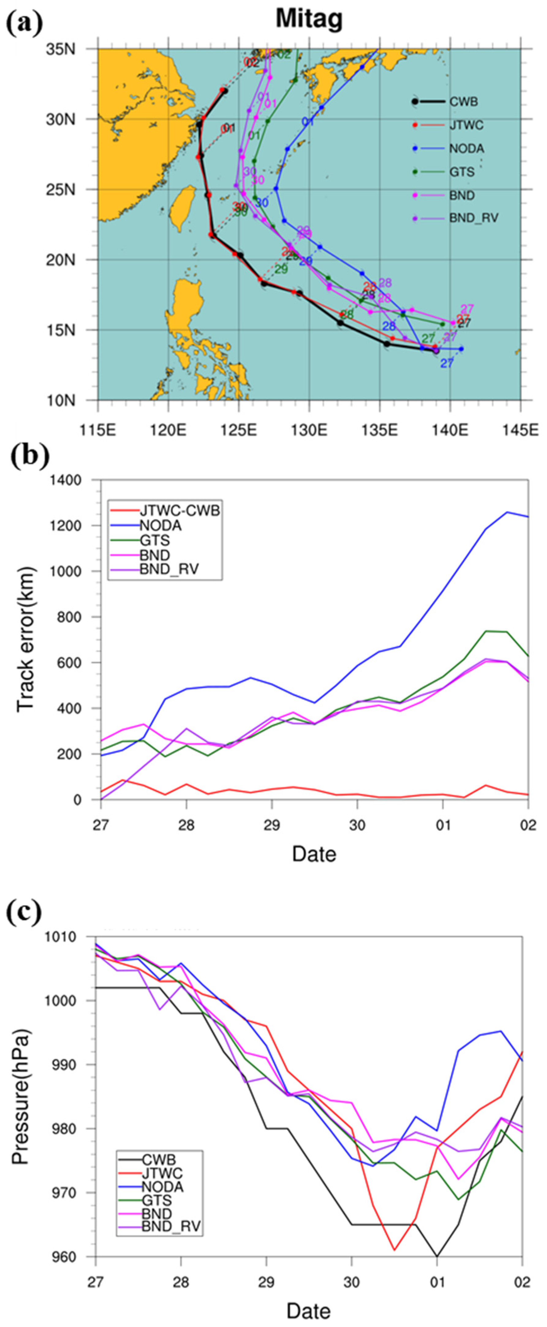
3.6. Impact on Forecast of Typhoon Mitag (2019)

The RO impact on typhoon forecast was also investigated by an extension to other cases occurring at later times when more RO data became available from FORMOSAT-7/COSMIC-2, a follow-on mission of FS3/C. For an illustration of the MPAS-GSI system performance, we chose one case, Typhoon Mitag (2019), that moved toward Taiwan at earlier stages, similar to Nepartak, but then took a north turn when nearing Taiwan. The experiment with the same model configurations as for Typhoon Nepartak was conducted with DA for 12 h till 0000 UTC 27 September 2019 and then followed by a forecast for 5 days. There are 3924 RO soundings available during the DA period. Figure 17 shows the forecasted tracks, track errors, and central sea-level pressure for NoDA, GTS, BND, and BND_RV for this case. All the forecasted tracks for the four experiments deviated northward from the best track since the initial time, but the GTS track becomes more eastward away from the observed (Figure 17a) leading to larger errors at the end forecast than both BND and BND_RV (Figure 17b). Note that NoDA using the NCEP FNL after the DA gives the largest track deviations, despite the fact that its initial typhoon center is closer to the observed. The vortex relocation in BND_RV enables the initial typhoon to closely collocate with the best track position, but the later track evolution is similar to that without the relocation in BND and both give similar track errors. For BND_RV with the V-match, the initial central sea-level pressure is improved but does not reach the best-track maximum intensity, which leads to a somewhat enhanced typhoon intensity only in the first two days. The later evolution of typhoon intensity for the four experiments, in general, is similar with pronounced underprediction (Figure 17c). It is probably due to the further northward track of the simulated typhoon that passes over the colder ocean as compared to the track of the observed typhoon over the warmer sea surface (not shown). Further analyses are needed to identify the factors for the slower typhoon intensification compared to the best track data of the Joint Typhoon Warning Center (JTWC). Although this example is not very stimulating for all forecasts, it essentially shows the sole impact of RO data assimilation with and without the DVI.

From the forecast results in Figure 17, a combination of both RO data assimilation and DVI still produces large eastward track deviations, despite the fact that the later track forecast has been improved. It is interesting to understand the performance of the BND experiment for this case. The geopotential height and horizontal wind at 850 hPa at 1200 UTC 26 September 2019 from the NCEP FNL dataset and the BND experiment after the first DA are shown in Figure 18. Compared to the FNL analysis, the location of the initial typhoon center in the BND experiment after the first DA is very close to the best track positions from CWB and JTWC (Figure 18b). After 12 h, the typhoon center shown by the FNL data deviated somewhat eastward from the best track positions of CWB and JTWC (Figure 18c); however, the typhoon center has a northeast shifting after the third DA cycle (Figure 18d) in association with a somewhat stronger and larger circulation compared to the global FNL analysis. It appears that the wind and associated zonal pressure gradient east of the typhoon center are stronger than the FNL analysis at this time and may induce a more northward typhoon movement in the forecast. Inclusion of the DVI with the vortex center relocated to the best track position does not fully remedy the biases in the wind analysis in the vicinity of the typhoon after DA, thus, still resulting in an eastward track deviation at earlier stages as seen in Figure 17. In addition to forecast sensitivity to initial analysis errors, track predictability is also tied to the relative performances of model physics schemes that affect the forecast skill as well. We did not examine an optimal combination of various physics schemes for use in MPAS in this study.

4. Conclusions

In this study, the 3DVAR/EnKF hybrid DA was integrated with the multi-resolution global model MPAS for typhoon forecasts with RO data assimilation lasting for two days to improve the initial condition. The hybrid DA consists of 36 ensemble members in GSI to update the background covariance with ensemble forecasts of MPAS at 120 km resolution and the 3DVAR to minimize the cost function for analysis used for the MPAS forecast at 60-15 km resolution to update analysis in continuous DA cycles at 6 h frequency. This is an approach with dual resolutions in the DA system. At the end of cycled assimilation, free forecasts of a total of 120 h were conducted for the experiments with different sets of GTS and RO data. Local bending angle and refractivity operators in GSI were used for RO data assimilation in the experiments, BND and REF, respectively, which are the same as the experiment GTS that assimilates all operationally available observations (including convectional radiosonde sounding data and satellite radiances) except for the RO data. In this study, we chose the typhoon case Nepartak (2016) to explore the impact of the RO data on typhoon track and intensity prediction, which can be compared with our previous work in Chen et al. [22] that applies the CWB global model for ensemble forecasts in the hybrid assimilation and the MPAS model for main forecasts. For improving the initial typhoon structure and intensity at the end of RO data assimilation, a dynamic vortex initialization (DVI) scheme that may effectively spin up the initial inner typhoon vortex through cycled model integration was applied to improve the typhoon vortex intensity and structure [13]. For the DVI, cycled runs of one hour using the forecast model continued to update the typhoon vortex until the typhoon reached the best track wind and pressure intensity, called V-match and P-match, respectively.

The two-way system reasonably captured the track and intensity of Nepartak with a forecast skill similar to the one-way system, both showing forecast improvement at earlier stages (days 1–3), but slightly degraded at later stages, when compared to the prediction using the global reanalysis at the end assimilation. The assimilation of additional RO data improved the track forecasts for REF and BND but has no appreciable impact on the intensity forecasts compared to GTS. Application of the DVI at the end of RO data assimilation largely improved the deepening rate of the typhoon before landfall at Taiwan for both REF and BND, but at cost of slightly increased track errors, especially for REF. Use of the DVI remains to be a preferred option with an acceptable trade-off, especially for GTS and BND. Use of a higher resolution of 60-15-3 km for BND further improved the intensity forecast, especially for the typhoon near landfall at day 4. The DVI at the higher resolution also further improved the intensity forecast with more consistent and stronger deepening rates, but with increased northward track deviations after day 3. The northward track deviations in some experiments were explained in this study using the wavenumber-one PV budget analysis, which is primarily dictated by PV horizontal advection compared to PV vertical advection and differential diabatic heating.

The feasibility of the 3DVAR/EnKF hybrid system (MPAS-GSI) was also illustrated in forecasts of Typhoon Mitag (2019) with more RO data available from FORMOSAT-7/COSMIC-2. The beneficial impacts of the combined DVI on forecast skill after assimilation of RO bending angle were presented for the two typhoon cases in this study. There are a number of factors that may greatly affect the impacts of RO observations on model forecast: better convective parameterization/cloud microphysics, better observation operators, more RO profiles, better RO profiles at lower altitudes, better background statistics, optimized bias correction on satellite radiance assimilation, and more blended assimilations with other observational data. In particular, typhoon forecasts can be further improved when available radar refractivity is assimilated in addition to RO data.

The current tests on the two selected cases are limited, however, and were reported for the purpose of presenting the feasibility of system development. This DA system, especially featured with the multi-resolution global model, will be applied to more typhoon forecasts with different combinations of physics schemes that also affect the forecasts. We will provide further evaluations for the performance of this DA system on more typhoon forecasts in association with RO data assimilation in another study.

References

1. Skamarock, W.C.; Klemp, J.B.; Duda, M.G.; Fowler, L.D.; Park, S.-H.; Ringler, T.D. A multiscale nonhydrostatic atmospheric model using centroidal Voronoi tesselations and C-grid staggering. Mon. Weather Rev. 2012, 140, 3090–3105. [Google Scholar] [CrossRef]
2. Huang, C.-Y.; Zhang, Y.; Skamarock, W.C.; Hsu, L.-H. Influences of large-scale flow variations on the track evolution of Typhoons Morakot (2009) and Megi (2010): Simulations with a global variable-resolution model. Month. Weather Rev. 2017, 145, 1691–1716. [Google Scholar] [CrossRef]
3. Huang, C.-Y.; Huang, C.-H.; Skamarock, W.C. Track deflection of typhoon Nesat (2017) as realized by multiresolution simulations of a global model. Month. Weather Rev. 2019, 147, 1593–1613. [Google Scholar] [CrossRef]
4. Kleist, D.T.; Parrish, D.F.; Derber, J.C.; Treadon, R.; Wu, W.-S.; Lord, S. Introduction of the GSI into the NCEP global data assimilation system. Weather Forecast. 2009, 24, 1691–1705. [Google Scholar] [CrossRef]
5. Shao, H.; Derber, J.; Huang, X.-Y.; Hu, M.; Newman, K.; Stark, D.; Lueken, M.; Zhou, C.; Nance, L.; Kuo, Y.-H. Bridging research to operations transitions: Status and plans of community GSI. Bull. Am. Meteorol. Soc. 2016, 97, 1427–1440. [Google Scholar] [CrossRef]
6. Hamill, T.M.; Snyder, C. A hybrid ensemble Kalman filter–3D variational analysis scheme. Month. Weather Rev. 2000, 128, 2905–2919. [Google Scholar] [CrossRef]
7. Schwartz, C.S.; Liu, Z.; Huang, X.-Y. Sensitivity of limited-area hybrid variational-ensemble analyses and forecasts to ensemble perturbation resolution. Month. Weather Rev. 2015, 143, 3454–3477. [Google Scholar] [CrossRef]
8. Kurihara, Y.; Bender, M.A.; Ross, R.J. An initialization scheme of hurricane models by vortex specification. Month. Weather Rev. 1993, 121, 2030–2045. [Google Scholar] [CrossRef]
9. Van Nguyen, H.; Chen, Y.-L. High-resolution initialization and simulations of Typhoon Morakot (2009). Month. Weather Rev. 2011, 139, 1463–1491. [Google Scholar] [CrossRef]
10. Van Nguyen, H.; Chen, Y.-L. Improvements to a tropical cyclone initialization scheme and impacts on forecasts. Month. Weather Rev. 2014, 142, 4340–4356. [Google Scholar] [CrossRef]
11. Cha, D.-H.; Wang, Y. A dynamical initialization scheme for real-time forecasts of tropical cyclones using the WRF model. Month. Weather Rev. 2013, 141, 964–986. [Google Scholar] [CrossRef]
12. Liu, H.-Y.; Wang, Y.; Xu, J.; Duan, Y. A dynamical initialization scheme for tropical cyclones under the influence of terrain. Weather Forecast. 2018, 33, 641–659. [Google Scholar] [CrossRef]
13. Huang, C.-Y.; Lin, J.-Y.; Skamarock, W.C.; Chen, S.-Y. Typhoon forecasts with dynamic vortex initialization using an unstructured mesh global model. Month. Weather Rev. 2022, in press. [Google Scholar] [CrossRef]
14. Kursinski, E.; Hajj, G.; Schofield, J.; Linfield, R.; Hardy, K.R. Observing Earth’s atmosphere with radio occultation measurements using the Global Positioning System. J. Geophys. Res. Atmos. 1997, 102, 23429–23465. [Google Scholar] [CrossRef]
15. Kuo, Y.-H.; Wee, T.-K.; Sokolovskiy, S.; Rocken, C.; Schreiner, W.; Hunt, D.; Anthes, R. Inversion and error estimation of GPS radio occultation data. J. Meteorol. Soc. Jpn. Ser. II 2004, 82, 507–531. [Google Scholar] [CrossRef]
16. Chu, C.-H.; Huang, C.-Y.; Fong, C.-J.; Chen, S.-Y.; Chen, Y.-H.; Yeh, W.-H.; Kuo, Y.-H. Atmospheric remote sensing using global navigation satellite systems: From FORMOSAT-3/COSMIC to FORMOSAT-7/COSMIC-2. Terr. Atmos. Ocean. Sci. 2021, 32, 1001–1013. [Google Scholar] [CrossRef]
17. Schreiner, W.S.; Weiss, J.; Anthes, R.A.; Braun, J.; Chu, V.; Fong, J.; Hunt, D.; Kuo, Y.H.; Meehan, T.; Serafino, W. COSMIC-2 radio occultation constellation: First results. Geophys. Res. Lett. 2020, 47, e2019GL086841. [Google Scholar] [CrossRef]
18. Ho, S.-P.; Zhou, X.; Shao, X.; Zhang, B.; Adhikari, L.; Kireev, S.; He, Y.; Yoe, J.G.; Xia-Serafino, W.; Lynch, E. Initial assessment of the COSMIC-2/FORMOSAT-7 neutral atmosphere data quality in NESDIS/STAR using in situ and satellite data. Remote Sens. 2020, 12, 4099. [Google Scholar] [CrossRef]
19. Chen, S.-Y.; Huang, C.-Y.; Kuo, Y.-H.; Guo, Y.-R.; Sokolovskiy, S. Assimilation of GPS refractivity from FORMOSAT-3/COSMIC using a nonlocal operator with WRF 3DVAR and its impact on the prediction of a typhoon event. Terr. Atmos. Ocean. Sci. 2009, 20, 133–154. [Google Scholar] [CrossRef]
20. Chen, Y.-C.; Hsieh, M.-E.; Hsiao, L.-F.; Kuo, Y.-H.; Yang, M.-J.; Huang, C.-Y.; Lee, C.-S. Systematic evaluation of the impacts of GPSRO data on the prediction of typhoons over the northwestern Pacific in 2008–2010. Atmos. Meas. Tech. 2015, 8, 2531–2542. [Google Scholar] [CrossRef] [Green Version]
21. Chen, S.-Y.; Zhao, H.; Huang, C.-Y. Impacts of GNSS radio occultation data on predictions of two super-intense typhoons with WRF hybrid variational-ensemble data assimilation. J. Aeronaut. Astronaut. Aviat 2018, 50, 347–364. [Google Scholar]
22. Chen, S.-Y.; Shih, C.-P.; Huang, C.-Y.; Teng, W.-H. An Impact Study of GNSS RO Data on the Prediction of Typhoon Nepartak (2016) Using a Multiresolution Global Model with 3D-Hybrid Data Assimilation. Weather Forecast. 2021, 36, 957–977. [Google Scholar]
23. Chen, S.-Y.; Nguyen, T.-C.; Huang, C.-Y. Impact of Radio Occultation Data on the Prediction of Typhoon Haishen (2020) with WRFDA Hybrid Assimilation. Atmosphere 2021, 12, 1397. [Google Scholar] [CrossRef]
24. Chen, X.M.; Chen, S.-H.; Haase, J.S.; Murphy, B.J.; Wang, K.-N.; Garrison, J.L.; Chen, S.-Y.; Huang, C.-Y.; Adhikari, L.; Xie, F. The impact of airborne radio occultation observations on the simulation of Hurricane Karl (2010). Month. Weather Rev. 2018, 146, 329–350. [Google Scholar] [CrossRef]
25. Cucurull, L. Improvement in the use of an operational constellation of GPS radio occultation receivers in weather forecasting. Weather Forecast. 2010, 25, 749–767. [Google Scholar] [CrossRef]
26. Cucurull, L.; Derber, J.; Purser, R. A bending angle forward operator for global positioning system radio occultation measurements. J. Geophys. Res. Atmos. 2013, 118, 14–28. [Google Scholar] [CrossRef]
27. Cucurull, L.; Derber, J.; Treadon, R.; Purser, R. Assimilation of global positioning system radio occultation observations into NCEP’s global data assimilation system. Month. Weather Rev. 2007, 135, 3174–3193. [Google Scholar] [CrossRef]
28. Huang, C.-Y.; Kuo, Y.-H.; Chen, S.-H.; Vandenberghe, F. Improvements in typhoon forecasts with assimilated GPS occultation refractivity. Weather Forecast. 2005, 20, 931–953. [Google Scholar] [CrossRef]
29. Huang, C.-Y.; Kuo, Y.-H.; Chen, S.-Y.; Terng, C.-T.; Chien, F.-C.; Lin, P.-L.; Kueh, M.-T.; Chen, S.-H.; Yang, M.-J.; Wang, C.-J. Impact of GPS radio occultation data assimilation on regional weather predictions. GPS Solut. 2010, 14, 35–49. [Google Scholar] [CrossRef]
30. Huang, C.-Y.; Chen, S.-Y.; Rao Anisetty, S.P.; Yang, S.-C.; Hsiao, L.-F. An impact study of GPS radio occultation observations on frontal rainfall prediction with a local bending angle operator. Weather Forecast. 2016, 31, 129–150. [Google Scholar] [CrossRef]
31. Yang, S.-C.; Chen, S.-H.; Chen, S.-Y.; Huang, C.-Y.; Chen, C.-S. Evaluating the impact of the COSMIC RO bending angle data on predicting the heavy precipitation episode on 16 June 2008 during SoWMEX-IOP8. Month. Weather Rev. 2014, 142, 4139–4163. [Google Scholar] [CrossRef]
32. Ha, S.; Snyder, C.; Skamarock, W.C.; Anderson, J.; Collins, N. Ensemble Kalman filter data assimilation for the Model for Prediction Across Scales (MPAS). Month. Weather Rev. 2017, 145, 4673–4692. [Google Scholar] [CrossRef]
33. Zhang, C.; Wang, Y. Projected future changes of tropical cyclone activity over the western North and South Pacific in a 20-km-mesh regional climate model. J. Clim. 2017, 30, 5923–5941. [Google Scholar] [CrossRef]
34. Hong, S.-Y.; Lim, J.-O.J. The WRF single-moment 6-class microphysics scheme (WSM6). Asia-Pac. J. Atmos. Sci. 2006, 42, 129–151. [Google Scholar]
35. Niu, G.Y.; Yang, Z.L.; Mitchell, K.E.; Chen, F.; Ek, M.B.; Barlage, M.; Kumar, A.; Manning, K.; Niyogi, D.; Rosero, E. The community Noah land surface model with multiparameterization options (Noah-MP): 1. Model description and evaluation with local-scale measurements. J. Geophys. Res. Atmos. 2011, 116. [Google Scholar] [CrossRef]
36. Hong, S.-Y.; Noh, Y.; Dudhia, J. A new vertical diffusion package with an explicit treatment of entrainment processes. Month. Weather Rev. 2006, 134, 2318–2341. [Google Scholar] [CrossRef]
37. Iacono, M.J.; Delamere, J.S.; Mlawer, E.J.; Shephard, M.W.; Clough, S.A.; Collins, W.D. Radiative forcing by long-lived greenhouse gases: Calculations with the AER radiative transfer models. J. Geophys. Res. Atmos. 2008, 113. [Google Scholar] [CrossRef]
38. Bannister, R. A review of operational methods of variational and ensemble-variational data assimilation. Q. J. R. Meteorol. Soc. 2017, 143, 607–633. [Google Scholar] [CrossRef]
39. Wang, X. Incorporating ensemble covariance in the gridpoint statistical interpolation variational minimization: A mathematical framework. Month. Weather Rev. 2010, 138, 2990–2995. [Google Scholar] [CrossRef]
40. Wang, X.; Parrish, D.; Kleist, D.; Whitaker, J. GSI 3DVar-based ensemble–variational hybrid data assimilation for NCEP Global Forecast System: Single-resolution experiments. Month. Weather Rev. 2013, 141, 4098–4117. [Google Scholar] [CrossRef]
41. Whitaker, J.S.; Hamill, T.M. Ensemble data assimilation without perturbed observations. Month. Weather Rev. 2002, 130, 1913–1924. [Google Scholar] [CrossRef]
42. Smith, E.K.; Weintraub, S. The constants in the equation for atmospheric refractive index at radio frequencies. Proc. IRE 1953, 41, 1035–1037. [Google Scholar] [CrossRef]
43. Born, M.; Wolf, E. Principles of Optics, 6th ed.; Pergamon: Oxford, UK, 1980; p. 808. [Google Scholar]
44. Barker, D. Southern high-latitude ensemble data assimilation in the Antarctic Mesoscale Prediction System. Month. Weather Rev. 2005, 133, 3431–3449. [Google Scholar] [CrossRef]
45. Barker, D.; Huang, X.-Y.; Liu, Z.; Auligné, T.; Zhang, X.; Rugg, S.; Ajjaji, R.; Bourgeois, A.; Bray, J.; Chen, Y. The weather research and forecasting model’s community variational/ensemble data assimilation system: WRFDA. Bull. Am. Meteorol. Soc. 2012, 93, 831–843. [Google Scholar] [CrossRef]
46. Hamill, T.M.; Whitaker, J.S.; Kleist, D.T.; Fiorino, M.; Benjamin, S.G. Predictions of 2010’s tropical cyclones using the GFS and ensemble-based data assimilation methods. Month. Weather Rev. 2011, 139, 3243–3247. [Google Scholar] [CrossRef]
47. Kleist, D.T. An Evaluation of Hybrid Variational-Ensemble Data Assimilation for the NCEP GFS; University of Maryland: College Park, Maryland, 2012. [Google Scholar]
48. Feng, J.; Wang, X. Impact of increasing horizontal and vertical resolution during the HWRF hybrid EnVar data assimilation on the analysis and prediction of Hurricane Patricia (2015). Month. Weather Rev. 2021, 149, 419–441. [Google Scholar] [CrossRef]
49. Lien, G.-Y.; Lin, C.-H.; Huang, Z.-M.; Teng, W.-H.; Chen, J.-H.; Lin, C.-C.; Ho, H.-H.; Huang, J.-Y.; Hong, J.-S.; Cheng, C.-P. Assimilation impact of early FORMOSAT-7/COSMIC-2 GNSS radio occultation data with Taiwan’s CWB Global Forecast System. Month. Weather Rev. 2021, 149, 2171–2191. [Google Scholar] [CrossRef]
50. Berrisford, P.; Kallberg, P.; Kobayashi, S.; Dee, D.; Uppala, S.; Simmons, A.; Poli, P.; Sato, H. Coauthors, 2011: The ERA-interim archive version 2.0. ERA Rep. Ser. 2019, 1, 23. [Google Scholar]
Figure 1. The flowchart of the GSI hybrid data assimilation. The data assimilation is divided into two parts that include the EnKF and GSI systems. The EnKF system uses n members (n is 36 in this study) at the lower resolution to provide background error covariances for the GSI system. The GSI system at the higher resolution provides the analysis for the EnKF system to re-center all ensemble members with the coarser resolution for MPAS forecasts, and then the new ensemble members can be updated for use in the next cycling.
Atmosphere 13 01353 g001
Figure 2. (a) The approximate mesh resolution of MPAS-60-15-3 km indicated by the contours at an interval of 3 km, and (b) the geometric locations of GPS RO soundings from 0000 UTC 2–4 July 2016 over the global MPAS mesh. The local region indicated by the black box is used for verification.
Atmosphere 13 01353 g002aAtmosphere 13 01353 g002b
Figure 3. (a) The vertical profiles of mean fractional differences (red line) in bending angle (i.e., (O−B)/B in %) and their standard deviations (blue line) between the observation (O) and the first guess (B) at different impact heights in the local verification region during the data assimilation of two days for BND, and (b) as in (a) but for the observation (O) and the analysis (A), i.e., (O−A)/A in %. (c,d) as in (a,b), respectively, but the fractional differences for REF. The black dashed line indicates the number of all GPS RO soundings (see the top axis) used in the local verification region.
Atmosphere 13 01353 g003
Figure 4. The averaged increments of the (a) temperature (shaded in K) and (b) specific humidity (shaded in g kg1) at 850 hPa during the data assimilation for the experiment GTS. (c,d) as in (a,b), respectively, but for REF. (e,f) as in (a,b), respectively, but for BND. The initial location of Typhoon Nepartak is indicated by the typhoon symbol. The locations of RO profiles used in the entire DA are plotted by solid points in (a,b).
Atmosphere 13 01353 g004
Figure 5. Geometric height (contours at an interval of 10 m), temperature (shaded in K), and wind vector (m s1) at 850 hPa at 0000 UTC 04 July 2016 (the end assimilation) for (a) the ERA-Interim, (b) GTS, (c) REF, and (d) BND.
Atmosphere 13 01353 g005
Figure 6. (a)The CWB best track (black) and the forecasted tracks for BND (pink line), REF (green line), GTS (blue line), and NoDA (red line) for Typhoon Nepartak. (b) as in (a) but for the evolution of the track errors with forecast time, and (c) as in (b) but for the central sea-level pressure of the typhoon.
Atmosphere 13 01353 g006aAtmosphere 13 01353 g006b
Figure 7. Geometric height (contours at an interval of 10 m), temperature (shaded in K), and horizontal wind (vectors in m s−1) at 850 hPa at 0000 UTC 07 July 2016 for (a) ERA-Interim, (b) GTS, (c) REF, and (d) BND.
Atmosphere 13 01353 g007
Figure 8. (a) The CWB best track (black line) and the forecasted tracks for BND (pink line), BND_RP (blue line), BND_RV (green line), and NoDA (red line) for Typhoon Nepartak. (d) as in (a) but for the track errors, and (g) as in (a) but for the central sea-level pressure error. (b,e,h) as in (a,d,g), respectively, but for REF. (c,f,i) as in (b,e,h), respectively, but for GTS. The numbers following the case names indicate the number of cycle runs.
Atmosphere 13 01353 g008
Figure 9. The daily-averaged forecast track errors (km) (average forecast errors at every six hours in the day) in five days against the best track for all experiments.
Atmosphere 13 01353 g009
Figure 10. Geometric height (contours at an interval of 10 m), temperature (shaded in K), and wind (vectors in m s−1) at 850 hPa at (a) 0000 UTC 4 July 2016 and (b) 0000 UTC 7 July 2016 for BND_RP.
Atmosphere 13 01353 g010
Figure 11. The differences in (a) potential temperature (shaded in K) and (b) specific humidity (shaded in g kg1) at 850 hPa between BND_RV and EC reanalysis at 0000 UTC 7 July 2016.
Atmosphere 13 01353 g011
Figure 12. The vertical profiles of mean fractional differences (red) in bending angle and their standard deviations (blue) between (a) the observation (O) and the first guess (B) during the data assimilation for BND_H (i.e., (O−B)/B in %) (similar to BND but with the resolution of 60-15-3 km), and (b) as in (a) but for the observation (O) and the analysis (A), i.e., (O−A)/A. The black dashed line indicates the number of all GPS RO soundings used in the verification area (see Figure 2) during the data assimilation. The vertical profiles are shown as impact height (km).
Atmosphere 13 01353 g012
Figure 13. (a) The CWB best track (black line) and the forecasted tracks for BND_H (blue line), BND_RVH (pink line), and BND_RPH (green line) for Typhoon Nepartak. (b) as in (a) but for the track errors with forecast time, and (c) as in (a) but for the central sea-level pressure. The numbers following the case names indicate the number of cycle runs.
Atmosphere 13 01353 g013
Figure 14. The differences in (a) potential temperature (shaded in K) and (b) specific humidity (shaded in g kg1) at 850 hPa between BND_RVH (with the higher resolution of 60-15-3 km) and the ERA-Interim at 0000 UTC 7 July 2016.
Atmosphere 13 01353 g014
Figure 15. The RMS forecast errors for BND_RVH (green), BND_RPH (blue), and BND_H (red) verified against the ERA-Interim for (a) potential temperature (in K) and (b) specific humidity (g kg−1), at 0000 UTC 7 July 2016.
Atmosphere 13 01353 g015
Figure 16. Wavenumber-one (WN-1) PV tendency budget (shaped colors in 10−5 PVU s−1) averaged at 1–8 km height at 0000 UTC 7 July 2016 for BND for (a) net PV budget, (b) PV horizontal advection, and (c) differential diabatic heating, with the overlaid WN-1 horizontal flow (vectors in m s−1). (df) are the same as (ac), respectively, but for BND_H. The regressed typhoon translation velocity (m s−1) is indicated by the vector at the typhoon center with the magnitude given at the lower right of each panel. A reference wind vector (m s−1) is given in the upper right for the WN-1 flow in each panel.
Atmosphere 13 01353 g016
Figure 17. (a) The CWB best track (black line), the JTWC best track (red line), and the forecast tracks for NoDA (blue line), GTS (green line), BND (pink line), and BND_RV (purple line) for Typhoon Mitag (2019) starting from 0000 UTC 27 September 2019. (b) as in (a) but for the track errors, and (c) as in (a) but for the central sea-level pressure. In (b), the red line shows the difference in the JTWC best track from the CWB best track.
Atmosphere 13 01353 g017
Figure 18. Geopotential height (contours at an interval of 10 gpm), wind speed (shaded in m s−1), and wind vectors (m s−1) at 850 hPa at 1200 UTC 26 September 2019 for (a) the NCEP FNL data and (b) after the first DA cycle. (c,d) as in (a,b), respectively, but at 0000 UTC 27 September 2019. The initial center position of Typhoon Mitag from the best track data of CWB and JTWC is indicated by the red typhoon sign and green typhoon sign, respectively.
Atmosphere 13 01353 g018