
Evaluation of GNSS Radio Occultation Profiles in the Vicinity of Atmospheric Rivers

Scripps Institution of Oceanography, University of California, San Diego, CA 92093, USA
*
Author to whom correspondence should be addressed.
Atmosphere 2022, 13(9), 1495; https://0-doi-org.brum.beds.ac.uk/10.3390/atmos13091495
Submission received: 12 July 2022
/
Revised: 29 August 2022
/
Accepted: 30 August 2022
/
Published: 14 September 2022
(This article belongs to the Special Issue Advances in GNSS Radio Occultation Technique and Applications)
Abstract
:Increasing the density of Global Navigation Satellite System radio occultation (RO) with commercial Smallsats and the next generation COSMIC-2 constellation is expected to improve analyses of the state of atmosphere, which is essential for numerical weather prediction. High vertical resolution RO profiles could be useful to observe atmospheric rivers (ARs) over the ocean, which transport water vapor in shallow, elongated corridors that frequently impact the west coasts of continents. The multi-year AR Reconnaissance campaign has extensively sampled ARs over the northeastern Pacific with dropsondes, providing an invaluable dataset to evaluate the reliability of RO retrievals. These dropsondes, and a reanalysis product that assimilates them, are compared to three RO datasets: (1) established operational missions, (2) COSMIC-2, and (3) the commercial Spire constellation. Each RO dataset has biases relative to reanalyses of less than 0.5% N in the upper troposphere and negative biases in the lower troposphere. Direct colocations with dropsondes indicate that vertical refractivity gradients present within ARs may be contributing to negative biases at higher altitudes inside than outside ARs, where the greatest variability and vertical gradients are at the well-defined boundary layer top. Observations from Spire are overly smooth, affecting the ability to resolve the low-level structure of an AR. Surprisingly, the depth of penetration into the lower troposphere is greater inside an AR than outside for all datasets. The results indicate that the observation errors used for assimilation of RO within ARs should consider the height dependent biases that are associated with the structure of the atmosphere.
1. Introduction
The vast majority (90%) of the meridional flux of water vapor in the middle latitudes occurs in narrow filaments called Atmospheric Rivers (ARs) [1]. The physical mechanism driving this flux of moisture in an AR is typically the strong winds in the low-level jet found ahead of the cold front in the warm sector of an extratropical cyclone (e.g., [2]). These low level weather phenomena are much more narrow (<1000 km) than they are long (>2000 km), with the core of an AR typically centered 1 km above the surface of the Earth and approximately 75% of the total transport of water vapor occurring in the lowest 3 km of the atmosphere (e.g., [2]). The main impacts from ARs are on the west coasts of continents in the middle latitudes (e.g., [3]), where they provide valuable contributions to the water supply [4,5,6,7,8]. However, they are also associated with extreme precipitation and most major flooding events in the western United States (e.g., [9,10,11,12,13]), as well as the most damage caused by flooding [14].
Despite great advances in numerical weather prediction (NWP) in the last few decades (e.g., [15,16]), major challenges remain in accurately forecasting the intensity and track of ARs. For example, in the ensemble system used by the European Centre for Medium-Range Weather Forecasts (ECMWF), on average only 75% of ensemble members accurately predict the location of AR landfall within 250 km for a two day lead time, dropping to less than 25% for a five day lead time [17]. An important step toward improving forecasts of ARs is more accurate analyses of the state of the atmosphere, as these analyses serve as the initial conditions for NWP models and errors tend to grow as a model is iterated forward due to the chaotic nature of the atmosphere [18]. Improving analyses is critical over the global oceans where in situ observations are relatively sparse (e.g., [19]). Observing moisture is particularly important over the oceans as sensitivity experiments employing an adjoint model have shown that errors in short-term forecasts of precipitation from landfalling ARs are highly sensitive to initial errors in the moisture within and near ARs [20,21,22,23].
A promising remote sensing technique for measuring the water vapor within ARs is Global Navigation Satellite System (GNSS) radio occultation (RO). The refractive bending of GNSS radio signals through the atmosphere is exploited in this technique as the signals are transmitted from GNSS constellations to receivers onboard low-Earth-orbiting (LEO) satellites [24]. The observed phase delays from these occulted signals are converted to profiles of bending angle and then into refractivity using an Abel transform [24,25], from which temperature and water vapor in the troposphere can be derived using the following relation:
where N is refractivity in N units, n is refractive index, P is atmospheric pressure in hPa, e is water vapor pressure in hPa, T is temperature in Kelvin, and the constants = 77.6 K hPa and = K hPa were derived empirically [26]. The result is a sounding of the thermodynamic structure of the atmosphere with high vertical resolution and little measurable interference from clouds and precipitation [27].
Observations from numerous GNSS RO missions have been used in research and operational NWP applications since it was first demonstrated in the Earth’s atmosphere by the Global Positioning System Meteorology (GPS/MET) mission [28]. The ambitious Formosa Satellite Mission 3 (FORMOSAT-3)/Constellation Observing System for Meteorology, Ionosphere and Climate (COSMIC-1) mission (hereafter COSMIC-1) [29] made the largest contribution to the number of global RO profiles available for operations until relatively recently, providing at least 1000 soundings per day over the period 2006–2016 and roughly triple this number during its peak years [30]. The addition of these RO observations to the suite of observations used in creating atmospheric analyses for global NWP systems has had a significant positive impact on forecasts [31,32,33,34,35,36,37,38], particularly in the stratosphere. Though the COSMIC-1 mission exceeded its planned lifetime by many years, it has now ceased operations, though other smaller missions are carrying on, in particular the European Organisation for the Exploitation of Meteorological Satellites (EUMETSAT)’s Meteorological Operational satellites program (MetOp) satellites [39] which now provide approximately 1800 profiles per day.
The follow-on to the successful COSMIC-1 mission is the FORMOSAT-7/COSMIC-2 (hereafter COSMIC-2), which was launched in June 2019 and is focused on the tropics and subtropics, producing approximately 4000 RO profiles per day mostly between 35 N and 35 S [30,40,41]. The increase in the number of profiles collected is partially due to the advanced TriG RO Receiver System (TGRS) employed by COSMIC-2, which is able to receive signals from multiple GNSS constellations, whereas previous GNSS RO missions were limited to the United States of America’s Global Positioning System (GPS). The COSMIC-2 beam-forming antennas provide a significantly increased signal-to-noise ratio that is nearly double that of the COSMIC-1 mission and facilitate deeper penetration into the lower troposphere [40,41,42]. A comparison between retrievals of refractivity from COSMIC-2 with in situ observations derived from co-located radiosondes and dropsondes shows similar biases in the troposphere to that of previous missions, such as COSMIC-1, that is commonly attributed to the difficulty in tracking the GNSS signals in superrefraction and/or multipath conditions in the lowest troposphere, where the complete spectral spread of the signals is difficult to capture. COSMIC-2 has a positive mean bias in the middle latitudes of the Northern Hemisphere between 2 and 6 km peaking at 1% of N near 3 km and rapidly decreasing with height to −4% of N near the Earth’s surface [40]. Assimilation of COSMIC-2 RO profiles into the operational Navy Global Environmental Model [NAVGEM; [43]] show comparable impact per observation to that of the GRAS receivers aboard the MetOp satellites [44]. Initial analysis of COSMIC-2 RO profiles assimilated into the ECMWF’s operational Integrated Forecast System (IFS) and NAVGEM models both show positive impacts on forecasts of temperature and winds, especially for short time ranges (12 h forecasts) in the core GNSS RO sampling heights of the upper troposphere and lower stratosphere, with the greatest regional impact in the Tropics where COSMIC-2 observations are concentrated [44,45]. These forecast improvements also extend to tropical humidity, as measured by radiosondes and radiances sensitive to tropospheric humidity from the Advanced Technology Microwave Sounder (ATMS).
Several companies in the private sector have designed piggy-back or dedicated missions to collect GNSS RO observations using receivers aboard their own commercial satellites in low Earth orbit. Among these companies, Spire has deployed enough small satellites to have amassed what is currently the largest constellation for Earth observation. They have been delivering approximately 7000 RO profiles per day during 2020 in near real time with global coverage [46]. The sharp increase in the number of global RO observations generated by Spire and other private companies has the potential to significantly improve NWP forecasts through data assimilation into NWP models due to their enormous volume (e.g., [47]). The impact of assimilating Spire RO observations into the United Kingdom Met Office Unified Model [48] was assessed by [49], who found a substantial benefit from their addition to the existing suite of global observations in their numerical experiments. Ref. [49] also found the difference between Spire RO observations and short-range forecasts (i.e., the innovations) to be comparable to the operational RO observations below 30 km, which did not include COSMIC-2 as they were not yet available at the time of their study. Initial results from the assimilation of Spire RO profiles into the NAVGEM show small positive impact on forecasts and comparable impact per observation to that of the COSMIC-1 mission [50].
Observing the lowest 3–5 km of the troposphere using GNSS-RO has proven challenging. This is due in part to atmospheric ducting at the top of the planetary boundary layer (PBL) which leads to a systematic negative bias in refractivity in RO retrievals at and below the top of the PBL [51]. While the ducting greatly complicates observing below the PBL, the large bending angle and sharp gradient in refractivity associated with this ducting provides a reliable way to detect the height of the PBL [52,53]. Techniques for correcting the negative bias in refractivity within the PBL have been proposed using collocated observations of total precipitable water [54], though this is only possible for the limited cases when these supplementary observations are available, or incorporating additional information from low-angle reflected GNSS-RO signals from the given occultation [55].
The goal of this study is to evaluate the performance of GNSS RO observations in the dynamically active environment in and around ARs and their associated extra-tropical cyclones. The various sources of spaceborne RO observations currently available for use in research and operations are compared to in situ observations from dropsondes collected during multi-year field campaigns over the northeast Pacific. The ability of RO to obtain accurate measurements, particularly in the lower troposphere within ARs, is described.
2. Data & Methods
2.1. Atmospheric River Reconnaissance
Weather reconnaissance flights targeting ARs have routinely taken place over the northeastern Pacific during the winter starting in 2018 as part of the AR Reconnaissance (AR Recon) program [56,57,58]. The main objective of AR Recon is to collect supplementary weather observations to aid and support NWP forecasts of the ARs that impact the west coast of North America and their associated precipitation. This is accomplished by sampling nascent and mature ARs and the weather features that drive them over the relatively data sparse northeastern Pacific Ocean. The primary observations collected in AR Recon are vertical profiles of temperature, moisture, and winds in the troposphere as sampled by dropsondes, and these observations have been shown to beneficially impact NWP forecasts [22,59]. In addition, profiles of refractivity retrieved from an airborne radio occultation (ARO) system [60] are also routinely collected during AR Recon, as well as observations of surface pressure from drifting buoys [61].
The present study utilizes a large dataset of 1334 dropsondes collected during AR Recon over the three recent winter seasons (starting in late January and continuing into March) of 2018, 2019, and 2020 (http://www.cw3e.ucsd.edu/ARRecon/, accessed on 20 March 2022). This includes observations from 29 intensive observing periods (IOPs) that were each centered around 0000 Coordinated Universal Time (UTC, approximately 1500 local standard time) from three aircraft, consisting of a combination of the National Oceanic and Atmospheric Administration(NOAA) G-IV and two United States Air Force C-130 aircraft, which have average cruising altitudes of 14 and 9 km, respectively. The aircraft flew 17 IOPs in AR Recon 2020 and six IOPs each during AR Recon 2018 & 2019. Not every IOP was associated with a distinct AR event; several sampled the same AR on different days. Prior to the 2019 campaign, the Vaisala RD94 model of dropsonde was used, afterwards it was replaced with the RD41 model with enhanced resolution [62]. The dropsondes have descent speeds of approximately 11 m s at sea level and 21 m s at 12 km altitude, with a resulting vertical resolution of 5–10 m. The top of each dropsonde profile is approximately 1 km below the altitude of the aircraft from which it was deployed and the lowest level of most profiles is 5–6 m above the surface. The precision of the measurements of pressure, temperature, and humidity are 0.01 hPa, 0.01 C, and 0.1 % and the uncertainties in these measurements are 0.4 hPa, 0.1 C, and 2 % respectively. The observed profiles from the dropsondes are converted to refractivity for comparison with RO observations using Equation (1). The ARO refractivity retrievals shown herein are from the 13 IOPs during AR Recon 2020 that included the NOAA G-IV equipped with the ARO system.
2.2. Spaceborne Radio Occultation
Three sources of GNSS radio occultations are compared in this study. The collection of GNSS RO observations that are used operationally by the National Center for Environmental Prediction (NCEP) for ingest into their Global Data Assimilation System (GDAS) system and subsequent assimilation into the Global Forecast System (GFS) model as of January 2020 are hereafter referred to as the operational dataset. This dataset was gathered from the COSMIC Data Analysis and Archive Center (CDAAC) archive and was comprised of the following GNSS RO missions during the period of study: COSMIC-1, Fifth Korea Multipurpose Satellite (KOMPSAT-5), MetOp-A, MetOp-B, MetOp-C, and the Radio Occultation and Heavy Precipitation (ROHP) experiment on board the Spanish Paz satellite. This operational dataset includes occultations from the GPS GNSS constellation only. Observations from the relatively recent COSMIC-2 mission were only available during AR Recon 2020. These observations were gathered from CDAAC’s COSMIC-2 Near Realtime dataset (https://data.cosmic.ucar.edu/gnss-ro/cosmic2/nrt/, accessed on 20 March 2022) and include occultations from signals emitted from both the GPS and Russian GLONASS GNSS constellations and are hereafter referred to as the COSMIC-2 dataset. Finally, the National Aeronautics and Space Administration (NASA) purchased commercial SmallSat RO observations from Spire for evaluation and made them available for use in this study. They are available for the period covering AR Recon 2019, and this dataset is hereafter referred to as the Spire dataset. This dataset includes occultations from the GPS, GLONASS, European Union’s Galileo, and Japan’s regional Quasi-Zenith Satellite System (QZSS) GNSS constellations.
Occultations from each of the aforementioned datasets were gathered over the northeast Pacific, defined here as 10–60, N & 170–100, W, over a 24 h period centered at 0000 UTC on the day of each IOP during AR Recon. Refractivity retrievals for each occultation were obtained from CDAAC and Spire in their atmPrf files, which are an output from the level 2 processing performed by these data providers. Observations that failed quality assurance as indicated in the atmPrf files were excluded from the analyses. In addition, clear outlier profiles from the COSMIC-2 dataset that had differences with the reanalysis product exceeding the threshold of 7% N above 5 km in altitude were excluded from the analyses; this additional step was not required for any other dataset.
For each occultation in the RO datasets any dropsondes within specified time and space thresholds were identified. The location of the lowest tangent point in the given RO and dropsonde profiles were used to determine the spatial separation.
2.3. Reanalysis
The reanalysis product chosen for this study is the ECMWF Renalysis 5 [ERA5; [63]]. It is available hourly on 37 pressure levels with a horizontal spatial resolution of 0.25× 0.25 (∼25–30 km) directly from the ECMWF archive. The ERA5 product is considered to provide one of the most accurate representations of tropospheric weather phenomenon in general (e.g., [64]) and for ARs in particular [65]. It also provides high temporal resolution with hourly output. The AR Recon dropsondes from the vast majority of IOPs were assimilated in real-time by the ECMWF and subsequently were included in the ERA5 product ([56], see Table 3) as were the GNSS RO observations from the operational dataset. RO observations from Spire were under evaluation and thus not yet available for assimilation by operational NWP centers during the period of this study and were not included in the ERA5 product. The RO observations from the COSMIC-2 dataset were not made available on the Global Telecommunication System until 16 March 2020 and were therefore not assimilated by operational weather prediction centers during AR Recon 2020 [45], and were also not included in the ERA5 product (Sean Healy 2020, personal communication).
For each dropsonde, a profile of refractivity was calculated from the ERA5 product from the nearest hour to the observation time using Equation (1). For each occultation, the reanalysis variables were extracted for the nearest hour to the observation time and for the nearest horizontal grid point to the latitude and longitude of each tangent point. Linear vertical interpolation was performed between the height of the two nearest vertical layers in the reanalysis product to the height of the given profile from a dropsonde or occultation for thermodynamic variables and logarithmic vertical interpolation was used for pressure. The result is an analysis profile with the same number of points as the observed occultation, with points that drift horizontally in the same manner as the given dropsonde or occultation.
Observed profiles were determined to be inside an AR when the vertically integrated vapor transport (IVT) calculated from the reanalysis product exceeded the commonly used threshold to identify ARs of 250 kg m s (e.g., [3]). The IVT criterion was placed on the vertical column of grid points in the reanalysis product containing the location of the lowest tangent point. The magnitude of IVT was calculated from the u and v components (zonal and meridional directions) of the IVT included with the ERA5 product.
2.4. Example Occultation/Dropsonde Pairs
In order to illustrate the quality of the RO observations, a qualitative comparison of occultations and dropsondes from each RO dataset is shown using pairs of occultations and dropsondes that were especially close in space and time. The first example pair includes an occultation from the operational dataset (the MetOp-C mission) that occurred during AR Recon 2020 IOP13 in the region poleward of a weak AR (Figure 1a). This occultation/dropsonde pair was just under 200 km apart in space and just under 2 h apart in time. The observations from the dropsonde are plotted in a standard Skew-T Log P diagram (Figure 1b) and show a relatively dry atmosphere above approximately 1.5 km above the surface, where a sharp low level temperature inversion is found. The refractivity derived from the observations from both the occultation and dropsonde are compared in Figure 1c, with the refractivity expressed as a difference from a zonal climatological profile for February at 27 N (i.e., observed N minus climatology N) extracted from CIRA-86 [66]. There is good agreement between the refractivity derived from these two observation types as well as their corresponding reanalysis profiles (dotted lines of the same color) for the extent of the profile. The occultation is truncated at approximately 3 km, likely due to a loss of the GNSS signal from multipath associated with the strong temperature inversion near this level, however it affects the signal for several km above the inversion.
The second example pair includes an occultation from the COSMIC-2 dataset that occurred during AR Recon 2020 IOP04 within the core of an intense AR with IVT exceeding 1000 kg m s (Figure 2a). This occultation/dropsonde pair was approximately 110 km apart in space and nearly simultaneous in time. In this case the observations from the dropsonde show a saturated environment within the core of the AR throughout the middle and lower troposphere with the temperature (red) and dew point temperature (blue) curves overlapping throughout these layers (Figure 1b). The refractivity from these two observation types differs greatly below approximately 8 km in height (Figure 1c), however both curves are similar to that of their corresponding reanalysis profiles (dotted lines). This shows that despite the observations being very close in time and space, the environment within the core of the AR is inhomogeneous, with large variations in refractivity on small spatial scales. The reanalysis product captures some of this variability, but there are significant differences remaining in the lower 2 km where the maximum in IVT transport is typically located and also in the height of the tropopause.
The final example pair includes an occultation from the Spire dataset that occurred during AR Recon 2019 IOP04 within the subtropical anticyclone often found off the coast of California (Figure 3a). This occultation/dropsonde pair was approximately 200 km apart in space and approximately 40 min apart in time. The observations from the dropsonde show a sharp temperature inversion near 1.5 km above the surface with very dry conditions above this level (Figure 3b), similar to what was shown in the first occultation/dropsonde pair (Figure 1b). The refractivity from the Spire occultation is very close to that of its paired dropsonde above approximately 3 km in altitude (Figure 3c), but these two observations differ greatly through the inversion layer where the occultation is very smooth and lacks the fine-scale vertical structure of the dropsonde or the occultations from the other datasets (Figure 1c and Figure 2c). The occultation from Spire also differs from the corresponding reanalysis profile (dotted line of the same color) below the temperature inversion, where the reanalysis profile roughly captures the boundary layer height and low level properties measured by the dropsonde. This smoothness found in the occultation from Spire compared to the other occultation datasets examined and also the dropsondes is found to be a common characteristic of the occultations from the Spire dataset examined in this study. While the Spire occultation does not match the dropsonde well in the lowest 3 km, it tends to produce an error that is closer to zero mean than the other RO missions, something to keep in mind as the statistics are analyzed below.
3. Results
It is commonly explained that RO profiles do not penetrate as deep into the troposphere in the tropics because the higher moisture there leads to a lower signal to noise ratio (SNR). This has been documented as far back as the initial GPS-Met mission [67] through to the COSMIC-1 mission [30]. The COSMIC-2 mission was designed to provide higher SNR to address this problem [41]. Section 3.1 explores whether that simple interpretation is also valid for atmospheric rivers, which would suggest that RO profiles would penetrate lower outside an AR than within the moisture-laden AR. The following sections compare co-located dropsondes and profiles from the three RO datasets, and then both observation types with the ERA5 reanalysis within and outside an AR.
3.1. Density of Sampling and Depth of Penetration of RO
The spatial density of the occultation datasets over the study region is shown in Table 1. The total samples column sums the number of occultations that were available in the northeastern Pacific Ocean study domain, for all days that had an AR Recon IOP, for the 24 h period centered at 0000 UTC each day. The average number of occultations per IOP was calculated by taking that total number of occultations (samples) and dividing by the number of IOPs, although the occultations may not have sampled near the AR that was targeted in the IOP. The density per IOP was calculated by dividing by the area of the study region in units of square degree of latitude and longitude. The Samples/IOP inside an AR (Table 2) divides the total number of profiles that sample areas with IVT greater than 250 kg m s by the number of IOPs.
The COSMIC-2 dataset contains roughly twice the number of occultations per IOP of the operational dataset over the study region, despite the fact that COSMIC-2 satellites are in a “tropical” orbit with maximum latitude of , and only covers the southern part of the study area. The Spire dataset contains just under half the number of the operational dataset. The density of occultations over the study region is relatively small in all datasets, with even the combined dataset only reaching 0.085 deg.
The distribution of data points with height for each of the occultation datasets is shown in Figure 4. The number of points that fell within each vertical bin of 200 m was calculated separately for profiles that sampled inside and also outside an AR (Figure 4a). It is evident from the number of observations per bin that many more occultation profiles were available from COSMIC-2 than from Spire dataset, with the number of profiles in the operational dataset falling between these two. All three datasets have many more observations per bin outside an AR than inside. The number of observations begins to decrease below approximately 6.5 km in height in the operational dataset, and all datasets rapidly decrease in number of samples with height below approximately 3 km.
The proportion of occultation profiles that sampled within each of the aforementioned vertical bins was calculated relative to the total number of occultations that sampled the topmost bin at 10 km for each dataset (Figure 4b). The proportion of occultations that are able to sample within the lowest 2 km of the atmosphere within an AR is higher than the proportion of occultations that sample within the lowest 2 km outside an AR, for each constellation. The COSMIC-2 dataset has the highest proportions throughout the lower troposphere, both inside and outside an AR. The operational dataset has much lower proportions of observations than the other datasets, not only in the lowest 2 km but in the region between 2 and 6 km, where the proportions in the COSMIC-2 and Spire datasets are both close to 100%. Inside an AR, the COSMIC-2 constellation has ∼5% higher proportion of occultations at 2 km than outside an AR, and 10% more at 1 km. Inside an AR, the Spire data set has about the same proportion of profiles as COSMIC-2 at 2 km, however it has about 10% lower proportion of profiles outside an AR at 1 km. Inside an AR, the operational dataset has ∼5% higher proportion of occultations at 2 km, than outside an AR, and ∼10% higher proportion of occultations at 1 km. The operational dataset also differs in the region between 2 and 6 km, where there are a higher proportion of observations outside an AR than inside. The general conclusion here is that RO samples deeper inside the high moisture environment of an AR than outside an AR. This is in stark contrast to generally accepted behavior in the moist tropical environment where RO sampling in the lowest troposphere is limited, and it is significant in that GNSS RO is performing well with respect to penetration in the region of most interest for forecasting ARs [20,21,22,23].
3.2. Comparison with Dropsondes
In order to evaluate the quality of the occultations, a quantitative comparison was made using the full dataset of occultation/dropsonde pairs where the occultations and their nearest dropsonde were within given thresholds in space and time. The statistics for a distance threshold of 300 km and a time threshold of 2 h are shown for each dataset in Figure 5. These thresholds are the same as was used in previous studies comparing occultations and dropsondes (e.g., [40]). For each pair, the difference between the profile of refractivity from the occultation and its corresponding dropsonde was calculated (occultation minus dropsonde) along with the percent difference in refractivity (grey lines). The mean (solid colored lines) and standard deviation (dashed colored lines) of these differences were also calculated using vertical bins of 200 m. These mean and standard deviation curves are also replotted in Figure 6 with each dataset shown in the same panel for ease of comparison.
For the 29 pairs identified in the operational dataset, the mean difference (bias) in refractivity is −1% near the surface (Figure 5a and Figure 6) and becomes positive at 1.42% near 2 km then quickly becomes negative at −1.3% near 3 km. Above 3.5 km the magnitude of the bias decreases to below 0.6% in absolute magnitude. The standard deviation is 2–4% N near the surface, increases to a maximum at 2 km of 4.8% N and steadily decreases with height to below 2% above 6.5 km. The negative bias near the surface (occultation minus dropsonde) represents a tendency for occultations to underestimate refractivity near the surface, as has been observed in other statistical studies for dropsondes and reanalysis [68].
For the 56 pairs identified in the COSMIC-2 dataset, the sign of the bias is negative throughout the lower half of the troposphere, with a maximum of −2.3% near the surface decreasing to 0.6% above 6.5 km (Figure 5b and Figure 6). The standard deviation of the COSMIC-2 dataset follows a similar pattern with height to that of the operational dataset but with much larger magnitude with a maximum of just over 7% near the surface and decreasing to 1% at 7 km. Profiles that were labeled with poor quality were excluded from the comparison, however the COSMIC-2 profile with over 30 % difference in refractivity in the lower troposphere in Figure 5b was not properly flagged in the NRT dataset, illustrating the need for additional quality checking at the ingest level.
For the 8 pairs identified in the Spire dataset the bias is positive in the lower troposphere in contrast to the other datasets examined (Figure 5c and Figure 6). This positive bias is near 2.8% near the surface, decreases to 0% at 1 km, then increases to 2.8% at 4 km, and decreases to below 0.5% above 7 km. The standard deviation of the differences is 3.8% near 1 km and slowly decreases to less than 1.5% above 5 km. Although the number of occultation/dropsonde pairs for the Spire dataset is small, the result indicates that the feature seen in Figure 3c due to oversmoothing contributes to a systematic positive bias, and will be investigated further in the ERA5 comparisons.
To get a qualitative indication of the relationship of occultation/dropsonde differences in the different regions of the AR environment, the comparison is broken down into occultation/dropsonde pairs where both observations are within an AR (Figure 7), and where both observations are outside an AR (Figure 8). There are not enough co-located pairs in each subset for quantitative analysis. Of note is the abrupt decrease in the bias in refractivity at 1.2 km for the COSMIC-2 dataset outside an AR, and the more gradual decrease in bias in this dataset starting at 4 km inside an AR. Negative biases in RO observations at low altitudes have been shown to be linked to sharp refractivity gradients. One cause is superrefraction of the RO signal at an interface where the gradient in refractivity exceeds a critical level, for example at a sharp boundary layer with a layer of low humidity above it. This leads to nonuniqueness in the retrieval process and underestimation of refractivity in the layers below the top of the boundary layer [69]. Another identified cause in the RO spectral inversion processing is the filtering of noise, if low amplitude subsignals due to atmospheric multipath propagation associated with variations in the gradient of refractivity are present. Subsignals that are not fully separable from the noise can also be unintentionally removed, which leads to a negative bias in refractivity [70].
The difference in the height at which the COSMIC-2 profiles begin to show this bias suggests that there are features within an AR that have strong gradients at higher levels than in the background maritime air mass found outside an AR. This is further explored in Figure 9, where the vertical gradients of refractivity (dN/dz) are calculated from the available dropsonde profiles and plotted as a function of height. There is a high occurrence of large negative dN/dz at 0.5–1.0 km for profiles outside an AR. The distribution of dN/dz in regions of the core of the AR with IVT > 500 kg m s is less than about ±250 N-units km above 3 km. Below about 3 km there is a distinct increase in the occurrence of profiles with larger negative refractivity gradient. This is approximately the height where COSMIC-2 profiles begin to show a consistent negative bias in refractivity in Figure 7b, whereas outside the AR the COSMIC-2 profiles begin to show a negative refractivity bias (Figure 8) closer to 1 km, where there is a high occurrence of large negative dN/dz. The fact that dN/dz within the core of the AR does not get as large as outside the AR helps to explain the conclusion that RO penetrates deeper within an AR than outside an AR as seen in Figure 4.
This would then imply that errors assigned to the RO observations are dependent on the background atmospheric structure. This is an important area to investigate, for example, it would affect how the observation errors used in data assimilation algorithms should be assigned. Without a significantly greater number of profile pairs, however, it is not possible to investigate this hypothesis directly Therefore, in the next section, we compare dropsondes to the ERA5 reanalysis product to establish that the ERA5 is accurately representing the key structure of an AR in the lower troposphere. Then, assuming the ERA5 captures that structure realistically, we search for any systematic biases in the RO datasets relative to the ERA5 inside and outside an AR. There are sufficient numbers of occultation profiles within an AR to carry out a more robust comparison using ERA5.
To attempt to create a larger and more robust dataset of occultation/dropsonde pairs, the statistics for the comparison in Figure 5 were recalculated using a distance threshold of 500 km and a time threshold of 4 h (Figure 10). With the relaxed threshold there were approximately triple the number of occultation/dropsonde pairs identified in each dataset to calculate the mean and standard deviation (Figure 11). The biases for all datasets now decrease more smoothly with height, however are greater near the surface (Figure 11). The COSMIC-2 dataset’s negative bias is −2.8% near the surface (Figure 10a) and the operational dataset is −1.8% near the surface (Figure 10b). The Spire dataset’s bias retains the large fluctuations with >2% near the surface, −1% at 2 km and 1.7% at 4 km (Figure 10c). The standard deviation is now similar for all datasets, with a maximum of 5.6% near 2 km (Figure 11), however that comes at the expense of mixing observations inside and outside an AR, and seems to be capturing the variability of the entire domain containing the AR rather than any systematic differences in errors. This further supports the approach of the next section to perform an indirect comparison of dropsondes to the ERA5 and then the ERA5 to the occultations. Subsets of occultation/dropsonde pairs inside and outside an AR for the increased distance and time thresholds are included for completeness in Figures S3 and S4.
While the number of dropsondes paired with the available spaceborne RO datasets is relatively small, there are many more dropsondes paired with the airborne RO (ARO) observations collected during AR Recon. There were 487 ARO profiles paired to dropsondes for the single season of AR Recon 2020 (Figure 12), which included 13 IOPs with ARO retrievals, for the same distance threshold of 300 km that was used for Figure 6. Most of these airborne occultations occurred within minutes of their paired dropsonde and thus represent the best possible representation of the level of agreement that is possible between the disparate datasets. The highest tangent points in each ARO profile are at the location of the aircraft when the occultation began, while the lower tangent points drift away from the aircraft. These airborne occultations have comparable bias in retrieved refractivity to that of the operational and COSMIC-2 datasets. In the lower troposphere, the airborne occultations have lower standard deviation with respect to dropsondes then the COSMIC-2 occultations, at 5% N compared to 6.5% N at 2 km, and comparable standard deviation to the operational RO dataset. ARO has slightly larger standard deviation than Spire, however the statistics are not as reliable for the small number of Spire profiles. The airborne occultations have higher standard deviations in the upper troposphere above 8 km, as is expected, due to the increased noise due to uncertainty in the velocity of the aircraft they are collected from [71,72].
3.3. Comparison with Reanalysis
This section explores further the characteristics of AR profiles in the lower troposphere inside and outside an AR. It is based on comparisons with reanalysis because there are not enough paired profiles to address this quantitatively in direct dropsonde to RO comparisons. The larger number of profiles included in the comparisons is interesting and informative, however there is a caveat in that the Operational RO and dropsondes were assimilated operationally into the ERA5 reanalysis, but the COSMIC-2 profiles and Spire profiles were not. Therefore one would anticipate that the agreement of Operational RO and dropsondes with ERA5 would be better than the other datasets. Given this caveat, the analysis focuses primarily on the features of the statistics as a function of height and their dynamical interpretation in addition to the absolute level of agreement.
3.3.1. Outside and Inside an Atmospheric River
A quantitative comparison between the reanalysis product and the dropsondes establishes the baseline statistics, with 537 dropsondes from AR Recon that sampled outside of an AR shown in Figure 13a and 820 dropsondes that sampled inside an AR shown in Figure 13b. The full refractivity profile derived from each dropsonde was calculated and then the reanalysis refractivity profile was subtracted. Above 5 km there are some positive differences, possibly because the dropsondes contain more detailed information about the tropopause height in the environment of the frontal systems than is present in the reanalysis. The mean of these differences (solid red lines) and the standard deviation (dotted red lines) are computed in vertical bins of 200 m.
The same quantitative comparison was made for the operational dataset for the 3008 occultations that sampled outside of an AR (Figure 14a) and 727 that sampled inside an AR (Figure 14b). The differences in refractivity (occultation minus reanalysis) increase considerably below approximately 7 km (Figure 14a) and are negative with a greater increase within an AR (Figure 14b). The mean difference curve becomes increasingly negative below 3 km in height.
The comparison for the COSMIC-2 dataset is shown for the 3445 occultations that sampled outside of an AR in Figure 15a and 1072 occultations inside an AR in Figure 15b. The differences between the observations and reanalysis (grey lines) follow a very similar pattern to that of the operational dataset with respect to height but with a larger standard deviation in the troposphere below 7 km.
The comparison for the Spire dataset is shown for the 291 occultations that sampled outside an AR in Figure 16a and the 51 occultations that samled inside an AR in Figure 16b. The differences between the observations and reanalysis (grey lines) follow a very different pattern to any other observational dataset examined. The mean difference curve (solid blue lines) have a shape that swings between positive and negative values with height with much more extreme changes outside an AR.
3.3.2. Intercomparison
The mean differences between the profiles in each of the observational datasets and their corresponding reanalysis profiles described above are plotted side-by-side for detailed comparison in Figure 17a. These statistics for the three RO datasets are also summarized in Tables S1–S3 with 1 km spacing in the vertical. The dropsonde dataset (red curves) has a positive bias from 1 to 2 km that suggests the reanalysis may not capture the sharp change in higher humidity below the boundary layer, and this feature is greater inside an AR than outside an AR. The dropsonde dataset has the smallest mean differences of the observational datasets examined in the range 2 to 5 km. There is a negative bias (lower refractivity, higher temperature) in the upper troposphere from approximately 5–9 km in altitude, reaching magnitudes of −0.25 and −0.5% N outside and within the AR, respectively, that is larger than the other datasets. The small systematic positive bias in refractivity of the dropsondes relative to the ERA5 reanalysis between 0.5 and 2 km of magnitudes of 0.2–0.5% N can be interpreted as the reanalysis product underestimating the moisture in the PBL, and this effect is greater within an AR than outside an AR. The fact there is no bias above 2 km indicates on average the ERA5 has little bias in the PBL height. It is interesting to consider this in terms of studies that have drawn attention to a systematic bias showing GPS RO derived PBL heights were higher than the ECMWF Interim Reanalysis [73] by 500 m [53,74]; the newer ERA5 product may agree better with RO derived PBL heights as well.
The profiles of mean differences for the COSMIC-2 and operational RO datasets are near zero above 3 km, and then are characterized by negative values below that in both datasets (Figure 17a). The positive bias with respect to the reanalysis found in the dropsonde dataset in the lower levels is not reproduced in the RO datasets. The largest negative mean differences are centered between 0.5 and 1 km for all RO datasets, with the largest magnitudes for COSMIC-2. In the COSMIC-2 and operational datasets, the mean difference is increasingly more negative inside an AR from 2 to 3 km. The mean differences for the occultation datasets all have a sharp decrease at 2 km, at approximately the top of the PBL. That negative bias is greatest for COSMIC-2 profiles outside an AR, and could be explained by a sharper gradient at the top of the PBL outside an AR. The trend toward a negative refractivity bias has been discussed frequently in the literature, due to the difficulty in reconstructing the full spectral content from all raypaths sampling into the PBL when the SNR is low [75]. The processing algorithms for the operational centers tend to take the approach of consistently retrieving bending angle until that SNR limit is reached.
In contrast, for the Spire dataset, the bias steeply increases downwards in the range 2–5 km, then decreases to negative values below 1 km. Inside an AR it decreases to −0.5% N and outside an AR it decreases more sharply to −1.2% N. Judging from the examples typical of Figure 3, Figure 5 and Figure 10, the Spire processing algorithm appears to favor smoothing out the entire profile below 4 km in order to achieve zero mean on average below 4 km, at the expense of severely contaminating the profile above 2 km with a positive bias. One could argue that the better approach would be to provide near zero mean bias observations above 2 km and reject or flag as questionable quality those below 2 km, rather than to provide biased observations over the entire range.
The standard deviation of the differences between the profiles in each of the observational datasets and their corresponding reanalysis are plotted side-by-side for detailed comparison in Figure 17b. All datasets have standard deviation of ∼0.5 to 0.6% N at the top of the profile with little variation until 7 km at which point the standard deviation increases more steeply and relatively smoothly towards the top of the PBL. We describe the differences among datasets by the value of the standard deviation at 2 km altitude, below which there is considerable variability in the behavior. The dropsonde dataset (red curves) has the smallest standard deviation of the observational datasets examined. The standard deviation at 2 km is ∼2% N outside an AR and ∼2.5% N inside an AR, then in both regions decreases to ∼1.5% N near the surface. We suggest that the large difference in standard deviation between 2 km and 7 km is due to high variability of moisture in the mid-levels within an AR that is difficult for the reanalysis to capture, even though the dropsondes have been assimilated into the ERA5. We suggest the reanalysis captures the moisture more accurately in the lowest level where it is controlled by the interaction with the sea surface and has less variability.
The profiles of standard deviation of the refractivity differences for the occultation datasets follow a similar pattern to that of the dropsonde dataset above 2 km (Figure 17b) and the overall magnitude is different for each dataset. All have greater standard deviation for profiles inside an AR, by 0.5 to 1.0% N, than outside an AR. The smallest standard deviations are found in the operational dataset, where both outside and within the AR above 2 km the magnitude of the deviations are very similar to that of the dropsondes. Below this level they are much larger than found in the dropsondes, at ∼2.5% N within and nearly ∼3% N outside an AR. This can be explained if one considers that the standard deviation for the RO datasets also includes variability of the atmosphere integrated along the horizontal raypath, so would be expected to be higher for RO than dropsonde point measurements. The largest standard deviations are found in the COSMIC-2 dataset, with values reaching ∼3% N at 2 km outside an AR and ∼3.3% N inside an AR. The standard deviations for the Spire dataset reach ∼3% N at 2 km outside an AR and ∼3.5% N inside an AR. The standard deviations for Spire have similar magnitudes to the dropsonde and operational dataset within an AR in the mid-troposphere between 7 km and 3 km, however much larger standard deviation below 3 km. As mentioned above, the two peaks of ∼3.5–4% N below 3 km appear to be associated with differences between the overly smoothed Spire profiles and the typical discontinuities present at the top of the PBL. In the lowest 2 km outside an AR, the operational, Spire, and COSMIC-2 standard deviation reach ∼2.8, 3.5 and 3.7% N, respectively. We suggest that all the occultation datasets are affected by the artifacts that produce the large negative biases noted earlier, and advise caution if these are to be used.
4. Analysis of the February 2019 Intense AR Event
The differences in refractivity inside versus outside an AR are explored using the example of the AR event that was sampled during AR Recon 2019 IOP03 on 13 February 2019 at 0000 UTC. This long-duration and high-intensity AR made landfall over California bringing AR4 conditions on the Atmospheric Rivers scale [76] and caused widespread impacts [77,78,79]. Figure 18 shows an overview of this IOP, which sampled the AR approximately one day before it made landfall using dropsondes from two aircraft (grey stars). The easternmost aircraft sampled a transect of the AR, and the westernmost aircraft sampled a transect reaching into the axis of the upper level trough (not shown). Several spaceborne RO observations (colored open circles) were paired with individual dropsondes (colored stars of the same color as its paired occultation) that occurred within 2 h and 500 km of the given occultation. Upper-level potential vorticity (PV) anomalies associated with upper-tropospheric waves have been shown to generate mesoscale frontal waves (MFWs) that affect the development and growth of extratropical cyclones and associated frontal systems and ARs [80,81,82]. In this case a MFW led to the formation of a secondary cyclone (evident in the closed mean sea level pressure contours to the north and northwest of the IVT maximum in Figure 18) and split the atmospheric river into two separate lobes of high IVT [79].
The easternmost transect of dropsondes, which passed through the region of maximum IVT (>1000 kg m s) within the AR, and then traversed the tail end of the second lobe of IVT, is plotted in Figure 19. The transect is depicted in terms of the observed temperature, humidity, and derived refractivity anomalies from the dropsondes, all shown relative to a zonal climatological profile at 27 N during February from CIRA-86 [66]. The transect of absolute temperature, humidity and refractivity is also shown in Supplemental Figure S5 along with the transect of winds from the dropsondes in Supplemental Figure S6. The profiles of refractivity anomaly derived from the occultations that were paired with the dropsondes in this transect are also overlain (green dashed lines) over their corresponding dropsonde. Along the transect horizontally, the characteristic poleward decrease in temperature and low level moisture (right to left in the figure) in baroclinic systems is apparent. In the vertical, there are few sharp gradients in temperature anomaly along the transect but there are many profiles with strong gradients in moisture anomaly, with these gradients becoming even more pronounced in the derived refractivity anomaly, which is a function of both variables.
A corresponding cross section through the ERA5 reanalysis product along the dropsonde transect but extending further poleward and equatorward is shown in Figure 20. The difference in the three dimensional refractivity field depicted by ERA5 and a monthly zonal climatology of refractivity at 27 N (referred to as the refractivity anomaly) is shaded. The location of the core of the AR is roughly in the center of the cross section at the 10th dropsonde profile counting from the left, at 25 N, within the low-level jet (Figure S6) on the equatorward side of the upward sloping frontal zone as indicated by the potential temperature contours (grey lines). The two lobes of IVT identified in Figure 18 are evident in the cross-section with the poleward-most (left side of the figure) lobe of IVT depicted as a shallowly dipping high refractivity (red shading) zone with a low level wind maximum at 1.5–2 km in Figure S6, and the equatorward IVT lobe depicted as a triangular zone of high refractivity with a low level wind maximum at 0.5–1.5 km altitude with a more steeply dipping northern boundary and a more shallow dipping boundary on the southern boundary showing the region of convective outflow. Outside of the AR on the equatorward side, high refractivity anomalies (red shading) are constrained to within the PBL (below approximately 2 km) and are capped by negative anomalies (blue shading) resulting in a large vertical gradient in refractivity near the top of the PBL. However, within the AR these high refractivity anomalies found near the surface extend to the middle troposphere, due to the moist convection and subsequent middle level moisture characteristic of the core of an AR (e.g., [2,62]). An example is shown in Figure 2, and statistically greater penetration is illustrated in Figure 4. Within the AR core, the environment is conducive to deeper penetration of RO profiles, without the extremely sharp vertical gradients of refractivity that are known to cause ducting and the loss of the GNSS signal beneath the PBL (e.g., [51]), and which appear so prominently in the distribution of extreme negative vertical refractivity gradients outside an AR in Figure 9a. Figure 9b–d show progressively lower occurrence of sharp vertical gradients of refractivity with higher IVT values in the AR core. We emphasize the vertical refractivity gradients because the nearly horizontal ray paths are susceptible to superrefraction if the angle of intersection with the layer is near critical at angles subparallel to the gradient. Although moderate horizontal gradients exist near the cold front and AR core, the raypaths are unlikely to be nearly subparallel to these gradients so unlikely to cause the severe atmospheric multipath often encountered in the case of strong gradients in the vertical.
Returning to the dropsonde transect in Figure 19, the two dropsondes that sampled the core of the AR along the transect (between 24.1 and 25.1 N) have relatively weak vertical gradients in both humidity and refractivity. These weak vertical gradients sampled by the dropsondes are depicted in the reanalysis cross section (Figure 20) by positive refractivity anomalies throughout the entire depth that the dropsondes sampled (lowest 8 km of the troposphere). There was no corresponding occultation paired to either of these dropsondes in the core of the AR, but the refractivity anomaly from the example occultation from the COSMIC-2 dataset that sampled the core of the AR during IOP04 of AR Recon 2020 (Figure 2) shows similar weak vertical gradients of refractivity and was able to sample down to the surface. The profiles on the flanks of the AR all have strong vertical variations in refractivity between 1 and 4 km in height, corresponding to the regions of negative refractivity anomalies (blue shading) directly adjacent to the AR core on the equatorward and poleward sides, respectively, in the reanalysis cross section. The paired occultation that sampled on the equatorward flank of the AR has a very similar refractivity profile to that of its corresponding dropsonde above 4 km and while it deviates a little bit below this level, it roughly follows the refractivity of the dropsonde before being cut off near 1 km, near the level of sharpest refractivity gradient associated with the top of the PBL. The paired occultation that sampled on the poleward flank of the AR reproduces the extreme refractivity variations between 0 and 5 km in height observed by its corresponding dropsonde. This pair sampled in the region of strongest refractivity gradient along the transect, indicated by the region of strong negative refractivity anomaly capping the positive refractivity anomaly in the PBL centered on 27 N. The transect from 29 to 15 N is very similar to the classical AR transect as described in [60], with the negative anomaly on the poleward side representing the cold air behind the cold front. However, this transect is more complicated in that on the poleward side of 29 the transect is cutting across the displaced frontal system associated with the mesolow to the northeast. Here the core of the shifted AR is seen in the sloping positive refractivity anomaly between 35 and 27 N. The shift in the AR core is evident in Figure 18 by the longer IVT vectors at the transect near the 5th dropsonde and 10th dropsonde (counting from the northwestern end of the transect).
5. Discussion
Of the RO datasets examined in this study the refractivity profiles from the operational dataset are the most similar to the refractivity derived from the dropsonde dataset. This is most evident in the comparison of the standard deviation curves with respect to the ERA5 reanalysis product for these two datasets (Figure 17b), where the curves are very similar in shape and magnitude until reaching 2 km in height, near the top of the boundary layer. This agreement is found both inside and outside an atmospheric river (AR) highlighting the consistency of the operational RO dataset. The very different magnitudes of the standard deviation curves in the COSMIC-2 and Spire RO datasets indicate that the general approach of using different observation errors as a function of height for each constellation in data assimilation is a reasonable approach (e.g., [83,84]).
The comparison of the state-of-the-science COSMIC-2 RO dataset to the reanalysis product has shown an overall similar shape of the mean bias and standard deviation curves to that of the operational RO dataset (Figure 17). However, the COSMIC-2 dataset has the largest negative biases in the lower troposphere as well as the largest standard deviations throughout most of the troposphere. The main differences between the COSMIC-2 and the previously launched RO missions that make up the operational RO dataset are (1) COSMIC-2 is more focused on tropical latitudes, (2) the advanced TGRS receiver employed by COSMIC-2, with its much higher signal-to-noise ratio (SNR), and (3) that the occultations from COSMIC-2 were not assimilated into the ERA5 product over the time period of this study. The TGRS receiver with higher SNR had been expected to provide more accurate data, and the source of this noise remains unresolved [41]. The consequence of not assimilating COSMIC-2 into ERA5 would have most effect in the upper troposphere (above 5 km), where the weighting of RO observations used in assimilation systems is much higher than in the lower troposphere. In the lower troposphere, RO observations are assigned large observation errors in the operational global models, including the ECMWF forecast model [44,85] on which the ERA5 reanalysis product is based. On the other hand, the dropsondes are assimilated in the ERA5, with smaller observation errors, and would have a stronger influence on the reanalysis. The larger negative biases and standard deviations in the lower troposphere could be related to COSMIC-2 sampling consistently deeper than the other RO datasets examined, due in part to its much higher signal-to-noise ratio. This successful reporting of deeper penetration of profiles would result in COSMIC-2 occultations more frequently encountering atmospheric super-refraction and ducting conditions, due to the presence of sharp temperature inversions, such as the trade wind inversion (e.g., [86], and strong horizontal gradients in moisture associated with the deep convection that characterizes the tropics.
The bias in the commercial Spire RO dataset with respect to the reanalysis product is radically different than that of any other RO dataset examined in this study throughout much of the troposphere. The operational and COSMIC-2 datasets have negative biases with respect to the reanalysis that peak near 0.5 km above the surface (Figure 17a), in general agreement with previous studies [29,40,41,42,51]. In contrast, the unusual pattern of bias in the Spire profiles reflects systemic differences in the occultations. The individual refractivity profiles from the Spire dataset are unrealistically smooth compared to that of the other RO datasets and also the dropsondes, with this being most evident in the lower troposphere and especially outside of an AR (see Figure 3c and grey lines in Figure 5, Figure 10 and Figure 16). The profiles in the Spire dataset smooth away the variability associated with the PBL, thus reducing the standard deviation; however, it produces a compensating positive and negative bias above and below the PBL, with the positive bias above the PBL unacceptably large. These apparently unphysical artifacts are possibly related to issues in the processing of the GNSS RO observable to retrieve refractivity, but what may be causing them is unclear as the details of the processing method employed are not made public by Spire. Despite these issues, recent numerical experiments using Spire RO profiles have shown them to have similar quality to operational RO observations and positive impact on forecasts [49,50]. This is likely due to the aforementioned general down weighting of RO observations in the lowest parts of the troposphere [32,44,85,87].
The RO datasets examined in this study all had very low spatial densities over the northeastern Pacific Ocean. The combined density of all RO datasets of 0.084 # deg is not sufficient for sampling within a given AR with enough occultations for detailed case studies and cross sections. Note that the density shown in Table 2 is actually an overestimate given that in the calculation the RO profile may have been in a different AR within the study region than the one being targeted in the IOP. The individual RO datasets all had very different spatial densities from one another. The COSMIC-2 dataset has more than double the average number of occultations per IOP of the operational dataset despite the COSMIC-2 mission being centered on the tropics and providing very few occultations poleward of 35 in the study region. These were often located in the general region of tropical moisture export, which can often have high IVT values, and not necessarily in the targeted AR. These densities of sampling will likely remain consistent for the operational and COSMIC-2 dataset but are likely underestimates of the current density of Spire occultations as more satellites have been added to this GNSS constellation. Additionally, Spire is only a single commercial GNSS constellation among several others that have been launched recently, so statistics in this study underestimate the density of commercial occultations considerably. Even with increases in the number of commercial RO observations, the use of an airborne radio occultation (ARO) system is the most effective way to consistently sample a given synoptic to mesoscale atmosphere feature like an AR with high spatial density at a given time [60].
6. Conclusions
Refractivity profiles derived from the COSMIC-2, Spire, and remaining operational GNSS radio occultation (RO) datasets were compared to dropsondes, and the ERA5 reanalysis product which assimilates them, in the dynamically active environments in and around atmospheric rivers (ARs) during winter in the northeastern Pacific. The results provide insight on the characteristics of RO profiles that are potentially useful, for example, to assess different observation error models and quality control criteria used to optimize assimilation of RO observations into the analyses used by numerical weather prediction models forecasting ARs. At present, these findings indicate that assimilation should consider the height dependent systematic differences among RO observations and other datasets that sample the structure of the atmosphere, especially in the lowest parts of the troposphere. To that effect, the results of the statistical comparisons are tabulated in the Supplementary Information to provide a guide for future efforts.
While the mean differences in refractivity between each of the observed datasets and the reanalysis product were less than approximately 0.5% N in the upper troposphere above 5 km, much larger differences were found in the lower troposphere. There the three RO datasets examined all have different characteristics, though they share a maximum negative bias, with respect to the reanalysis, below 1 km.
6.1. Comparison of RO with Dropsondes
- COSMIC-2 refractivity observations are biased low relative to dropsondes, with the bias becoming more negative near the surface, whereas the operational RO dataset is closer to zero mean. The standard deviation for COSMIC-2 relative to dropondes is almost twice as big as the standard deviation for the operational RO dataset.
- Although the number of RO profiles from Spire collocated with dropsondes is relatively samll, comparisons show the Spire profiles are overly smooth in the lower troposphere with radically different characteristics than the other RO constellations, affecting the ability to resolve sharp boundaries. In consequence, the bias of refractivity profiles from Spire relative to dropsondes that would normally be expected to exist only below the boundary layer, for example, tend to contaminate the profiles at higher altitudes, and specifically contaminates the profiles difference with the reanalysis up to 5 km in height.
- Refractivity gradients are smaller in absolute magnitude within the core of an AR than they are in the surrounding environment, leading to deeper penetration of RO profiles within the AR than outside an AR.
- Based on limited collocations, the COSMIC-2 bias relative to dropsondes abruptly decreases at 2.8 km inside an AR and decreases at 1.2 km outside an AR. These heights correspond to where the variations in the vertical gradient of refractivity (dN/dz) become larger and more negative.
- Regions with relatively high moisture at mid-levels, such as beneath the convective outflow within an AR and behind and near the cold front, effectively lift the height of the maximum vertical gradient of refractivity and tend to reduce it. This is in contrast to regions with a well-defined top of the planetary boundary layer (PBL) and little middle level moisture above, such as adjacent to an AR, which have a much lower and larger maximum vertical gradient in refractivity.
6.2. Comparison of Dropsondes with Reanalysis
- The dropsonde dataset showed a positive mean difference with respect to the ERA5 reanalysis of 0.5% N between 1 and 2 km indicating a potential dry bias of ERA5 below the PBL in this environment. In contrast, the three RO datasets had large negative bias with respect to ERA5 greater than −1% N below 1 km, making it unrealistic to expect they are reliable at these levels without further study.
- The standard deviation of the difference between the dropsonde and reanalysis product peaks at 2 km, approximately at the PBL height, and decreases to 1.5% N at the surface. This may indicate that the general decrease in apparent error at about 0.5–1 km often observed in GNSS RO datasets may be realistic and may not be an artifact of the reduced number of profiles (i.e., [83]).
- The standard deviation of the difference between the dropsonde dataset and reanalysis is approximately 0.5–1% N larger within an AR than outside over the height range 1.5–6 km. This indicates the ERA5 does not capture the full variability of humidity within an AR. The operational RO dataset closely follows this pattern above 2 km.
6.3. Comparison of RO with Reanalysis
- The standard deviation of the differences with the reanalysis product for the three RO datasets is nearly constant above 7.5 km and increases approximately linearly towards the surface, peaking between 1 and 2 km. In general the differences follow the type of error model described in [83] but suggest a lower observational error could be used in this AR environment in the range 7.5 to 10 km than is commonly assumed for operational models [88,89].
- The standard deviation of the difference with the reanalysis for the dropsonde and the three RO datasets are all larger inside an AR compared to outside, with the largest values in the COSMIC-2 and Spire datasets.
- The individual refractivity profiles within the Spire dataset are extremely smooth compared to that of the other RO datasets and dropsondes, particularly in the lower troposphere, and are likely contributing to the artifacts seen in the mean difference.
- The COSMIC-2 and Spire RO datasets have much larger standard deviations than that of the operational RO and dropsonde datasets throughout most of the troposphere, with the largest values found in the COSMIC-2 dataset. Spire and COSMIC-2 reach a standard deviation of ∼3.5% N below 2 km, compared to ∼2.8% N for operational RO.
6.4. Characteristics in the Lowest Parts of the Troposphere
- The negative refractivity bias relative to reanalysis below 1 km is larger outside an AR than inside an AR for all three RO datasets. This may indicate that super-refraction or ducting may be worse outside the AR where the refractivity gradient is sharper at the top of the PBL.
- The depth of penetration among the RO datasets is highest in the COSMIC-2 dataset with >90% of occultations reaching down to 1 km, next highest in the Spire dataset (>85% at 1 km), and the lowest in the operational dataset (>65% at 1 km).
- The depth of penetration into the lower troposphere is greater inside an AR than outside in all RO datasets examined. There are approximately 10% more profiles reaching 1 km above the surface inside an AR than outside an AR in all datasets.
- The deeper penetration of RO within an AR is likely due to the fact that the distribution of the vertical gradient in refractivity (dN/dz) is narrower (i.e., less than 500 N-units km) for dropsondes within the AR core where integrated vapor transport (IVT) is >750 kg m s, and progressively wider for lower values of IVT. This could be due to a reduction in dN/dz from greater mixing of humidity into higher levels by moist convection within the core of an AR, compared to outside an AR where there is less variation above the very strong refractivity gradients at the top of the PBL.
Supplementary Materials
The following supporting information can be downloaded at: https://0-www-mdpi-com.brum.beds.ac.uk/article/10.3390/atmos13091495.
Author Contributions
Conceptualization, J.S.H.; Formal analysis, M.J.M.J. and J.S.H.; Funding acquisition, J.S.H.; Methodology, M.J.M.J., J.S.H.; Project administration, J.S.H.; Investigation, M.J.M.J.; Resources, J.S.H.; Software, M.J.M.J.; Data curation, M.J.M.J.; Supervision, J.S.H.; Validation, M.J.M.J.; Visualization, M.J.M.J.; Writing—original draft, M.J.M.J. and J.S.H.; Writing—review & editing, M.J.M.J., J.S.H. All authors have read and agreed to the published version of the manuscript.
Funding
This work was supported by NSF Grant AGS-1642650 and AGS-1454125, NASA Grant NNX15AU19G. Support was also provided by the Center for Western Weather and Water Extremes (CW3E), the Atmospheric River Program of the California Department of Water Resources, and the US Army Corps of Engineers Forecast-Informed Reservoir Operations Program.
Data Availability Statement
The reanalysis products were retrieved from the European Center for Medium-range Weather Forecasting (ECMWF), available from https://0-doi-org.brum.beds.ac.uk/10.24381/cds.bd0915c6 and accessed on 20 March 2022. The operational and COSMIC-2 occultation data was provided by the COSMIC Data Analysis and Archive Center (CDAAC), available from https://www.cosmic.ucar.edu/what-we-do/cosmic-2/data and accessed on 20 March 2022. The Spire occultation data was provided under an exclusive use purchase by NASA and made available through NASA Grant NNX15AU19G. The dropsonde data were provided by the CW3E, NOAA and the US Air Force, available at https://seb.noaa.gov/pub/acdata and accessed on 20 March 2022. The ARO data is available at https://agsweb.ucsd.edu/airborne_ro and accessed on 20 March 2022. The authors thank the CW3E staff, B. Kawzenuk and R. Demirdjian, for facilitating access to the CW3E dropsonde and other data.
Acknowledgments
The authors thank B. Cao for assistance with incorporating the ARO observations and comments on the manuscript. Resources supporting this work were provided by the NASA High-End Computing (HEC) Program and we thank S.-H. Chen for assistance with the use of those facilities. The authors thank the scientists from the UCAR COSMIC Program office and Spire for useful discussions regarding the datasets.
Conflicts of Interest
The funders had no role in the design of the study; in the collection, analyses, or interpretation of data; in the writing of the manuscript, or in the decision to publish the results.
References
- Zhu, Y.; Newell, R.E. A Proposed Algorithm for Moisture Fluxes from Atmospheric Rivers. Mon. Weather Rev. 1998, 126, 725–735. [Google Scholar] [CrossRef]
- Ralph, F.M.; Iacobellis, S.F.; Neiman, P.J.; Cordeira, J.M.; Spackman, J.R.; Waliser, D.E.; Wick, G.A.; White, A.B.; Fairall, C. Dropsonde Observations of Total Integrated Water Vapor Transport within North Pacific Atmospheric Rivers. J. Hydrometeorol. 2017, 18, 2577–2596. [Google Scholar] [CrossRef]
- Guan, B.; Waliser, D.E. Detection of atmospheric rivers: Evaluation and application of an algorithm for global studies. J. Geophys. Res. Atmos. 2015, 120, 12514–12535. [Google Scholar] [CrossRef]
- Guan, B.; Molotch, N.P.; Waliser, D.E.; Fetzer, E.J.; Neiman, P.J. Extreme snowfall events linked to atmospheric rivers and surface air temperature via satellite measurements. Geophys. Res. Lett. 2010, 37. [Google Scholar] [CrossRef]
- Dettinger, M.D.; Ralph, F.M.; Das, T.; Neiman, P.J.; Cayan, D.R. Atmospheric Rivers, Floods and the Water Resources of California. Water 2011, 3, 445–478. [Google Scholar] [CrossRef]
- Ralph, F.M.; Coleman, T.; Neiman, P.J.; Zamora, R.J.; Dettinger, M.D. Observed Impacts of Duration and Seasonality of Atmospheric-River Landfalls on Soil Moisture and Runoff in Coastal Northern California. J. Hydrometeorol. 2013, 14, 443–459. [Google Scholar] [CrossRef]
- Rutz, J.J.; Steenburgh, W.J.; Ralph, F.M. Climatological characteristics of atmospheric rivers and their inland penetration over the western United States. Mon. Weather Rev. 2014, 142, 905–921. [Google Scholar] [CrossRef]
- Adusumilli, S.; Fish, M.; Fricker, H.A.; Medley, B. Atmospheric River Precipitation Contributed to Rapid Increases in Surface Height of the West Antarctic Ice Sheet in 2019. Geophys. Res. Lett. 2021, 48. [Google Scholar] [CrossRef]
- Ralph, F.M.; Neiman, P.J.; Wick, G.A.; Gutman, S.I.; Dettinger, M.D.; Cayan, D.R.; White, A.B. Flooding on California’s Russian River: Role of atmospheric rivers. Geophys. Res. Lett. 2006, 33. [Google Scholar] [CrossRef]
- Lavers, D.A.; Allan, R.P.; Wood, E.F.; Villarini, G.; Brayshaw, D.J.; Wade, A.J. Winter floods in Britain are connected to atmospheric rivers. Geophys. Res. Lett. 2011, 38. [Google Scholar] [CrossRef] [Green Version]
- Lavers, D.A.; Villarini, G.; Allan, R.P.; Wood, E.F.; Wade, A.J. The detection of atmospheric rivers in atmospheric reanalyses and their links to British winter floods and the large-scale climatic circulation. J. Geophys. Res. Atmos. 2012, 117. [Google Scholar] [CrossRef]
- Stohl, A.; Forster, C.; Sodemann, H. Remote sources of water vapor forming precipitation on the Norwegian west coast at 60 N–a tale of hurricanes and an atmospheric river. J. Geophys. Res. Atmos. 2008, 113. [Google Scholar] [CrossRef]
- Viale, M.; Nuñez, M.N. Climatology of winter orographic precipitation over the subtropical central Andes and associated synoptic and regional characteristics. J. Hydrometeorol. 2011, 12, 481–507. [Google Scholar] [CrossRef]
- Corringham, T.W.; Ralph, F.M.; Gershunov, A.; Cayan, D.R.; Talbot, C.A. Atmospheric rivers drive flood damages in the western United States. Sci. Adv. 2019, 5, eaax4631. [Google Scholar] [CrossRef]
- Bauer, P.; Thorpe, A.; Brunet, G. The quiet revolution of numerical weather prediction. Nature 2015, 525, 47–55. [Google Scholar] [CrossRef]
- Alley, R.B.; Emanuel, K.A.; Zhang, F. Advances in weather prediction. Science 2019, 363, 342–344. [Google Scholar] [CrossRef]
- DeFlorio, M.J.; Waliser, D.E.; Guan, B.; Lavers, D.A.; Ralph, F.M.; Vitart, F. Global Assessment of Atmospheric River Prediction Skill. J. Hydrometeorol. 2018, 19, 409–426. [Google Scholar] [CrossRef]
- Lorenz, E.N. The predictability of a flow which possesses many scales of motion. Tellus 1969, 21, 289–307. [Google Scholar] [CrossRef]
- Ota, Y.; Derber, J.C.; Kalnay, E.; Miyoshi, T. Ensemble-based observation impact estimates using the NCEP GFS. Tellus A Dyn. Meteorol. Oceanogr. 2013, 65, 20038. [Google Scholar] [CrossRef]
- Doyle, J.D.; Amerault, C.; Reynolds, C.A.; Reinecke, P.A. Initial condition sensitivity and predictability of a severe extratropical cyclone using a moist adjoint. Mon. Weather Rev. 2014, 142, 320–342. [Google Scholar] [CrossRef]
- Reynolds, C.A.; Doyle, J.D.; Ralph, F.M.; Demirdjian, R. Adjoint sensitivity of North Pacific atmospheric river forecasts. Mon. Weather Rev. 2019, 147, 1871–1897. [Google Scholar] [CrossRef]
- Stone, R.E.; Reynolds, C.A.; Doyle, J.D.; Langland, R.H.; Baker, N.L.; Lavers, D.A.; Ralph, F.M. Atmospheric River Reconnaissance Observation Impact in the Navy Global Forecast System. Mon. Weather Rev. 2020, 148, 763–782. [Google Scholar] [CrossRef]
- Demirdjian, R.; Doyle, J.D.; Reynolds, C.A.; Norris, J.R.; Michaelis, A.C.; Ralph, F.M. A Case Study of the Physical Processes Associated with the Atmospheric River Initial-Condition Sensitivity from an Adjoint Model. J. Atmos. Sci. 2020, 77, 691–709. [Google Scholar] [CrossRef]
- Kursinski, E.; Hajj, G.; Schofield, J.; Linfield, R.; Hardy, K.R. Observing Earth’s atmosphere with radio occultation measurements using the Global Positioning System. J. Geophys. Res. Atmos. 1997, 102, 23429–23465. [Google Scholar] [CrossRef]
- Hajj, G.A.; Kursinski, E.; Romans, L.; Bertiger, W.; Leroy, S. A technical description of atmospheric sounding by GPS occultation. J. Atmos. Sol.-Terr. Phys. 2002, 64, 451–469. [Google Scholar] [CrossRef]
- Smith, E.K.; Weintraub, S. The Constants in the Equation for Atmospheric Refractive Index at Radio Frequencies. Proc. IRE 1953, 41, 1035–1037. [Google Scholar] [CrossRef]
- Solheim, F.S.; Vivekanandan, J.; Ware, R.H.; Rocken, C. Propagation delays induced in GPS signals by dry air, water vapor, hydrometeors, and other particulates. J. Geophys. Res. Atmos. 1999, 104, 9663–9670. [Google Scholar] [CrossRef]
- Kursinski, E.R.; Hajj, G.A.; Bertiger, W.; Leroy, S.; Meehan, T.; Romans, L.; Schofield, J.; McCleese, D.; Melbourne, W.; Thornton, C.; et al. Initial results of radio occultation observations of Earth’s atmosphere using the Global Positioning System. Science 1996, 271, 1107–1110. [Google Scholar] [CrossRef]
- Anthes, R.A.; Bernhardt, P.; Chen, Y.; Cucurull, L.; Dymond, K.; Ector, D.; Healy, S.; Ho, S.P.; Hunt, D.; Kuo, Y.H.; et al. The COSMIC/FORMOSAT-3 mission: Early results. Bull. Am. Meteorol. Soc. 2008, 89, 313–334. [Google Scholar] [CrossRef]
- Ho, S.P.; Anthes, R.A.; Ao, C.O.; Healy, S.; Horanyi, A.; Hunt, D.; Mannucci, A.J.; Pedatella, N.; Randel, W.J.; Simmons, A.; et al. The COSMIC/FORMOSAT-3 radio occultation mission after 12 years: Accomplishments, remaining challenges, and potential impacts of COSMIC-2. Bull. Am. Meteorol. Soc. 2020, 101, E1107–E1136. [Google Scholar] [CrossRef] [Green Version]
- Healy, S. Forecast impact experiment with a constellation of GPS radio occultation receivers. Atmos. Sci. Lett. 2008, 9, 111–118. [Google Scholar] [CrossRef]
- Healy, S. Surface pressure information retrieved from GPS radio occultation measurements. Q. J. R. Meteorol. Soc. 2013, 139, 2108–2118. [Google Scholar] [CrossRef]
- Aparicio, J.M.; Deblonde, G. Impact of the assimilation of CHAMP refractivity profiles on Environment Canada global forecasts. Mon. Weather Rev. 2008, 136, 257–275. [Google Scholar] [CrossRef]
- Poli, P.; Moll, P.; Puech, D.; Rabier, F.; Healy, S.B. Quality control, error analysis, and impact assessment of FORMOSAT-3/COSMIC in numerical weather prediction. TAO Terr. Atmos. Ocean. Sci. 2009, 20, 1. [Google Scholar] [CrossRef]
- Cucurull, L. Improvement in the use of an operational constellation of GPS radio occultation receivers in weather forecasting. Weather Forecast. 2010, 25, 749–767. [Google Scholar] [CrossRef]
- Rennie, M. The impact of GPS radio occultation assimilation at the Met Office. Q. J. R. Meteorol. Soc. J. Atmos. Sci. Appl. Meteorol. Phys. Oceanogr. 2010, 136, 116–131. [Google Scholar] [CrossRef]
- Bonavita, M. On some aspects of the impact of GPSRO observations in global numerical weather prediction. Q. J. R. Meteorol. Soc. 2014, 140, 2546–2562. [Google Scholar] [CrossRef]
- Bauer, P.; Radnóti, G.; Healy, S.; Cardinali, C. GNSS radio occultation constellation observing system experiments. Mon. Weather. Rev. 2014, 142, 555–572. [Google Scholar] [CrossRef]
- von Engeln, A.; Healy, S.; Marquardt, C.; Andres, Y.; Sancho, F. Validation of operational GRAS radio occultation data. Geophys. Res. Lett. 2009, 36. [Google Scholar] [CrossRef]
- Ho, S.P.; Zhou, X.; Shao, X.; Zhang, B.; Adhikari, L.; Kireev, S.; He, Y.; Yoe, J.G.; Xia-Serafino, W.; Lynch, E. Initial Assessment of the COSMIC-2/FORMOSAT-7 Neutral Atmosphere Data Quality in NESDIS/STAR Using In Situ and Satellite Data. Remote Sens. 2020, 12, 4099. [Google Scholar] [CrossRef]
- Schreiner, W.S.; Weiss, J.; Anthes, R.A.; Braun, J.; Chu, V.; Fong, J.; Hunt, D.; Kuo, Y.H.; Meehan, T.; Serafino, W.; et al. COSMIC-2 radio occultation constellation: First results. Geophys. Res. Lett. 2020, 47, e2019GL086841. [Google Scholar] [CrossRef]
- Chen, S.Y.; Liu, C.Y.; Huang, C.Y.; Hsu, S.C.; Li, H.W.; Lin, P.H.; Cheng, J.P.; Huang, C.Y. An Analysis Study of FORMOSAT-7/COSMIC-2 Radio Occultation Data in the Troposphere. Remote Sens. 2021, 13, 717. [Google Scholar] [CrossRef]
- Hogan, T.F.; Liu, M.; Ridout, J.A.; Peng, M.S.; Whitcomb, T.R.; Ruston, B.C.; Reynolds, C.A.; Eckermann, S.D.; Moskaitis, J.R.; Baker, N.L.; et al. The Navy Global Environmental Model. Oceanography 2014, 27, 116–125. [Google Scholar] [CrossRef]
- Ruston, B.; Healy, S. Forecast impact of FORMOSAT-7/COSMIC-2 GNSS radio occultation measurements. Atmos. Sci. Lett. 2021, 22, e1019. [Google Scholar] [CrossRef]
- Healy, S. ECMWF starts assimilating COSMIC-2 data. ECMWF Newsl. 2020, 163, 5–6. [Google Scholar]
- Masters, D.; Duly, T.; Esterhuizen, S.; Irisov, V.; Jales, P.; Nguyen, V.; Nogués-Correig, O.; Tan, L.; Yuasa, T.; Angling, M. GNSS-Based Earth Observations from the Growing Spire Nanosatellite Constellation. In Lecture given at the 5th International Conference on GPS Radio Occultation; National Space Organization: Hsinchu, Taiwan, 2020; p. AB076. [Google Scholar]
- Harnisch, F.; Healy, S.; Bauer, P.; English, S. Scaling of GNSS radio occultation impact with observation number using an ensemble of data assimilations. Mon. Weather Rev. 2013, 141, 4395–4413. [Google Scholar] [CrossRef]
- Walters, D.; Brooks, M.; Boutle, I.; Melvin, T.; Stratton, R.; Vosper, S.; Wells, H.; Williams, K.; Wood, N.; Allen, T.; et al. The Met Office unified model global atmosphere 6.0/6.1 and JULES global land 6.0/6.1 configurations. Geosci. Model Dev. 2017, 10, 1487–1520. [Google Scholar] [CrossRef]
- Bowler, N. An assessment of GNSS radio occultation data produced by Spire. Q. J. R. Meteorol. Soc. 2020, 146. [Google Scholar] [CrossRef]
- Ruston, B. GNSS-RO Use with the NAVGEM System. In Lecture given at the 5th International Conference on GPS Radio Occultation; National Space Organization: Hsinchu, Taiwan, 2020; p. AB081. [Google Scholar]
- Ao, C.O.; Meehan, T.; Hajj, G.; Mannucci, A.; Beyerle, G. Lower troposphere refractivity bias in GPS occultation retrievals. J. Geophys. Res. Atmos. 2003, 108. [Google Scholar] [CrossRef]
- Xie, F.; Wu, D.; Ao, C.; Mannucci, A.; Kursinski, E. Advances and limitations of atmospheric boundary layer observations with GPS occultation over southeast Pacific Ocean. Atmos. Chem. Phys. 2012, 12, 903–918. [Google Scholar] [CrossRef]
- Ao, C.O.; Waliser, D.E.; Chan, S.K.; Li, J.L.; Tian, B.; Xie, F.; Mannucci, A.J. Planetary boundary layer heights from GPS radio occultation refractivity and humidity profiles. J. Geophys. Res. Atmos. 2012, 117. [Google Scholar] [CrossRef] [Green Version]
- Wang, K.N.; de la Torre Juárez, M.; Ao, C.O.; Xie, F. Correcting negatively biased refractivity below ducts in GNSS radio occultation: An optimal estimation approach towards improving planetary boundary layer (PBL) characterization. Atmos. Meas. Tech. 2017, 10, 4761–4776. [Google Scholar] [CrossRef]
- Wang, K.N.; Ao, C.O.; Juarez, M.d.l.T. GNSS-RO Refractivity Bias Correction Under Ducting Layer Using Surface-Reflection Signal. Remote Sens. 2020, 12, 359. [Google Scholar] [CrossRef]
- Ralph, F.M.; Cannon, F.; Tallapragada, V.; Davis, C.A.; Doyle, J.D.; Pappenberger, F.; Subramanian, A.; Wilson, A.M.; Lavers, D.A.; Reynolds, C.A.; et al. West Coast forecast challenges and development of atmospheric river reconnaissance. Bull. Am. Meteorol. Soc. 2020, 101, E1357–E1377. [Google Scholar] [CrossRef]
- Zheng, M.; Delle Monache, L.; Wu, X.; Ralph, F.M.; Cornuelle, B.; Tallapragada, V.; Haase, J.S.; Wilson, A.M.; Mazloff, M.; Subramanian, A.; et al. Data gaps within atmospheric rivers over the northeastern Pacific. Bull. Am. Meteorol. Soc. 2021, 102, E492–E524. [Google Scholar] [CrossRef]
- Cobb, A.; Ralph, F.M.; Tallapragada, V.; Wilson, A.M.; Davis, C.A.; Monache, L.D.; Doyle, J.D.; Pappenberger, F.; Reynolds, C.A.; Subramanian, A.; et al. Atmospheric River Reconnaissance 2021: A Review. Weather Forecast. 2022. [Google Scholar] [CrossRef]
- Zheng, M.; Delle Monache, L.; Cornuelle, B.D.; Ralph, F.M.; Tallapragada, V.S.; Subramanian, A.; Haase, J.S.; Zhang, Z.; Wu, X.; Murphy, M.J.; et al. Improved forecast skill through the assimilation of dropsonde observations from the Atmospheric River Reconnaissance program. J. Geophys. Res. Atmos. 2021, 126, e2021JD034967. [Google Scholar] [CrossRef]
- Haase, J.; Murphy, M.; Cao, B.; Ralph, F.; Zheng, M.; Delle Monache, L. Multi-GNSS Airborne Radio Occultation Observations as a Complement to Dropsondes in Atmospheric River Reconnaissance. J. Geophys. Res. Atmos. 2021, 126, e2021JD034865. [Google Scholar] [CrossRef]
- Centurioni, L.R. Drifter technology and impacts for sea surface temperature, sea-level pressure, and ocean circulation studies. In Observing the Oceans in Real Time; Springer: Berlin/Heidelberg, Germany, 2018; pp. 37–57. [Google Scholar]
- Cobb, A.; Michaelis, A.; Iacobellis, S.; Ralph, F.; Delle Monache, L. Atmospheric River Sectors: Definition and Characteristics Observed Using Dropsondes from 2014 to 20 CalWater and AR Recon. Mon. Weather Rev. 2021, 149, 623–644. [Google Scholar] [CrossRef]
- Hersbach, H.; Bell, B.; Berrisford, P.; Hirahara, S.; Horányi, A.; Muñoz-Sabater, J.; Nicolas, J.; Peubey, C.; Radu, R.; Schepers, D.; et al. The ERA5 global reanalysis. Q. J. R. Meteorol. Soc. 2020, 146, 1999–2049. [Google Scholar] [CrossRef]
- Mahto, S.S.; Mishra, V. Does ERA-5 outperform other reanalysis products for hydrologic applications in India? J. Geophys. Res. Atmos. 2019, 124, 9423–9441. [Google Scholar] [CrossRef]
- Cobb, A.; Delle Monache, L.; Cannon, F.; Ralph, F. Representation of Dropsonde-Observed Atmospheric River Conditions in Reanalyses. Geophys. Res. Lett. 2021, 48, e2021GL093357. [Google Scholar] [CrossRef]
- Kirchengast, G.; Hafner, J.; Poetzi, W. The CIRA-86aQ_UoG Model: An Extension of the CIRA-86 Monthly Tables including Humidity Tables and a Fortran95 Global Moist Air Climatology Model. 1999. Available online: https://cir.nii.ac.jp/crid/1570291225144589056 (accessed on 11 July 2022).
- Poli, P.; Joiner, J.; Kursinski, E.R. 1DVAR analysis of temperature and humidity using GPS radio occultation refractivity data. J. Geophys. Res. Atmos. 2002, 107, ACL 14-1–ACL 14-20. [Google Scholar] [CrossRef]
- Schreiner, W.; Sokolovskiy, S.; Hunt, D.; Rocken, C.; Kuo, Y.H. Analysis of GPS radio occultation data from the FORMOSAT-3/COSMIC and Metop/GRAS missions at CDAAC. Atmos. Meas. Tech. 2011, 4, 2255–2272. [Google Scholar] [CrossRef]
- Sokolovskiy, S. Effect of superrefraction on inversions of radio occultation signals in the lower troposphere. Radio Sci. 2003, 38. [Google Scholar] [CrossRef]
- Sokolovskiy, S.; Rocken, C.; Schreiner, W.; Hunt, D. On the uncertainty of radio occultation inversions in the lower troposphere. J. Geophys. Res. Atmos. 2010, 115. [Google Scholar] [CrossRef]
- Muradyan, P.; Haase, J.S.; Xie, F.; Garrison, J.L.; Voo, J. GPS/INS navigation precision and its effect on airborne radio occultation retrieval accuracy. GPS Solut. 2011, 15, 207–218. [Google Scholar] [CrossRef]
- Xie, F.; Haase, J.S.; Syndergaard, S. Profiling the atmosphere using the airborne GPS radio occultation technique: A sensitivity study. IEEE Trans. Geosci. Remote Sens. 2008, 46, 3424–3435. [Google Scholar] [CrossRef]
- Dee, D.P.; Uppala, S.M.; Simmons, A.J.; Berrisford, P.; Poli, P.; Kobayashi, S.; Andrae, U.; Balmaseda, M.; Balsamo, G.; Bauer, d.P.; et al. The ERA-Interim reanalysis: Configuration and performance of the data assimilation system. Q. J. R. Meteorol. Soc. 2011, 137, 553–597. [Google Scholar] [CrossRef]
- Guo, P.; Kuo, Y.H.; Sokolovskiy, S.; Lenschow, D. Estimating atmospheric boundary layer depth using COSMIC radio occultation data. J. Atmos. Sci. 2011, 68, 1703–1713. [Google Scholar] [CrossRef]
- Wang, K.N.; Garrison, J.L.; Acikoz, U.; Haase, J.S.; Murphy, B.J.; Muradyan, P.; Lulich, T. Open-loop tracking of rising and setting GPS radio-occultation signals from an airborne platform: Signal model and error analysis. IEEE Trans. Geosci. Remote Sens. 2016, 54, 3967–3984. [Google Scholar] [CrossRef]
- Ralph, F.M.; Rutz, J.J.; Cordeira, J.M.; Dettinger, M.; Anderson, M.; Reynolds, D.; Schick, L.J.; Smallcomb, C. A Scale to Characterize the Strength and Impacts of Atmospheric Rivers. Bull. Am. Meteorol. Soc. 2019, 100, 269–289. [Google Scholar] [CrossRef]
- Hatchett, B.J.; Cao, Q.; Dawson, P.B.; Ellis, C.J.; Hecht, C.W.; Kawzenuk, B.; Lancaster, J.; Osborne, T.; Wilson, A.M.; Anderson, M.; et al. Observations of an Extreme Atmospheric River Storm With a Diverse Sensor Network. Earth Space Sci. 2020, 7, e2020EA001129. [Google Scholar] [CrossRef]
- Chen, S.; Reynolds, C.A.; Schmidt, J.M.; Papin, P.P.; Janiga, M.A.; Bankert, R.; Huang, A. The Effect of a Kona Low on the Eastern Pacific Valentine’s Day (2019) Atmospheric River. Mon. Weather Rev. 2022. [Google Scholar] [CrossRef]
- Hecht, C.W.; Michaelis, A.C.; Martin, A.C.; Cordeira, J.M.; Cannon, F.; Ralph, F.M. Illustrating Ensemble Predictability across Scales Associated with the 13–15 February 2019 Atmospheric River Event. Bull. Am. Meteorol. Soc. 2022, 103, E911–E922. [Google Scholar] [CrossRef]
- Ralph, F.M.; Neiman, P.J.; Kiladis, G.N.; Weickmann, K.; Reynolds, D.W. A Multiscale Observational Case Study of a Pacific Atmospheric River Exhibiting Tropical—-Extratropical Connections and a Mesoscale Frontal Wave. Mon. Weather Rev. 2011, 139, 1169–1189. [Google Scholar] [CrossRef]
- Martin, A.C.; Ralph, F.M.; Wilson, A.; DeHaan, L.; Kawzenuk, B. Rapid cyclogenesis from a mesoscale frontal wave on an atmospheric river: Impacts on forecast skill and predictability during atmospheric river landfall. J. Hydrometeorol. 2019, 20, 1779–1794. [Google Scholar] [CrossRef]
- Michaelis, A.C.; Martin, A.C.; Fish, M.A.; Hecht, C.W.; Ralph, F.M. Modulation of atmospheric rivers by mesoscale frontal waves and latent heating: Comparison of two US West Coast events. Mon. Weather Rev. 2021, 149, 2755–2776. [Google Scholar] [CrossRef]
- Chen, S.Y.; Huang, C.Y.; Kuo, Y.H.; Sokolovskiy, S. Observational error estimation of FORMOSAT-3/COSMIC GPS radio occultation data. Mon. Weather Rev. 2011, 139, 853–865. [Google Scholar] [CrossRef]
- Bowler, N.E. Revised GNSS-RO observation uncertainties in the Met Office NWP system. Q. J. R. Meteorol. Soc. 2020, 146, 2274–2296. [Google Scholar] [CrossRef]
- Healy, S.; Thépaut, J.N. Assimilation experiments with CHAMP GPS radio occultation measurements. Q. J. R. Meteorol. Soc. J. Atmos. Sci. Appl. Meteorol. Phys. Oceanogr. 2006, 132, 605–623. [Google Scholar] [CrossRef]
- Riehl, H.; Yeh, T.; Malkus, J.; Laseur, N. The northeast trade of the Pacific Ocean. Q. J. R. Meteorol. Soc. 1951, 77, 598–626. [Google Scholar] [CrossRef]
- Chen, S.; Huang, C.; Kuo, Y.; Guo, Y.; Sokolovskiy, S.; Stract, A.B. Assimilation of GPS Refractivity from FORMOSAT-3/COSMIC Using a Nonlocal Operator with WRF 3DVAR and Its Impact on the Prediction of a Typhoon Event. Terr. Atmos. Ocean. Sci. 2009, 20, 133–154. [Google Scholar] [CrossRef]
- Cucurull, L.; Derber, J. Operational implementation of COSMIC observations into NCEP’s global data assimilation system. Weather Forecast. 2008, 23, 702–711. [Google Scholar] [CrossRef]
- Ruston, B. Considerations for GNSS-RO Bending Angle Observation Error. JCSDA Q. 2019, 62, 18–21. [Google Scholar] [CrossRef]
Figure 1.
An example occultation from the operational dataset (MetOp-C mission) that was just under 200 km apart in space and just under 2 h apart in time. (a) Overview of the thirteenth intensive observing period (IOP13) of AR Recon 2020 with integrated vapor transport (kg m s, shaded and vectors) and mean sea level pressure (hPa, grey contours) shown. The locations of dropsondes are indicated by grey stars and occultations from the operational, and COSMIC-2 datasets are indicated by green, and purple circles, respectively, with each of their collocated dropsondes indicated by enlarged stars of the same color. The location of the occultation/dropsonde pair highlighted for this example is circled in light blue. (b) A standard Skew-T Log P diagram of the data collected by the dropsonde in the example pair with the dry bulb temperature indicated by the red curve and dew point temperature indicated by the blue curve. (c) The difference in refractivity (% N) between a zonal climatology during February at 27 N and the example occultation (solid green line), its nearest dropsonde (solid red line), and their corresponding reanalysis profiles (dotted lines of the same color as their observation).

Figure 2.
Same as Figure 1 but for an example occultation from the COSMIC-2 dataset (purple) that was approximately 110 km apart in space and nearly simultaneous in time during the fourth intensive observing period (IOP04) of AR Recon 2020.
Figure 2.
Same as Figure 1 but for an example occultation from the COSMIC-2 dataset (purple) that was approximately 110 km apart in space and nearly simultaneous in time during the fourth intensive observing period (IOP04) of AR Recon 2020.

Figure 3.
Same as Figure 2 but for an example occultation from the Spire dataset (blue) that approximately 200 km apart in space and approximately 40 min apart in time during the fourth intensive observing period (IOP04) of AR Recon 2019.
Figure 3.
Same as Figure 2 but for an example occultation from the Spire dataset (blue) that approximately 200 km apart in space and approximately 40 min apart in time during the fourth intensive observing period (IOP04) of AR Recon 2019.

Figure 4.
Comparison of (a) total count (# bin) and (b) proportion of the total count (% bin) of radio occultation observations in vertical bins (200 m width) for each dataset both within (dashed lines) and outside (solid lines) the atmospheric river. The operational (green lines), COSMIC-2 (purple lines), and Spire (blue lines) datasets are shown.

Figure 5.
Statistical comparison between occultations and their nearest AR Recon dropsonde that was within a distance threshold of 300 km and a time threshold of 2 h. The percent difference in refractivity (% of N) is shown between each occultation in the (a) operational, (b) COSMIC-2, and (c) Spire dataset and its corresponding dropsonde profile (grey lines), along with the mean and standard deviation of these differences (solid and dashed colored lines, respectively) computed in vertical bins with width of 200 m. The thick dashed black line highlights the line of zero difference and the number of sample pairs, n, for each dataset is indicated.

Figure 6.
Comparison of the (a) mean and (b) standard deviation of the percent difference in refractivity between each of the observed datasets and their nearest AR Recon dropsonde that was within a distance threshold of 300 km and a time threshold of 2 h. The operational (green lines), COSMIC-2 (purple lines), and Spire (blue lines) datasets are shown. The thick dashed black line in panel (a) highlights the line of zero difference.

Figure 7.
The percent difference (occultation minus dropsonde) in refractivity (% N) for pairs from the (a) operational, (b) COSMIC-2, and (c) Spire dataset where both observations were inside an AR and were within a distance threshold of 300 km and a time threshold of 2 h. Labels are the same as Figure 5.

Figure 8.
Same as Figure 7 but for occultation-dropsonde pairs that were outside an AR and were within a distance threshold of 300 km and a time threshold of 2 h. Labels are the same as Figure 6.

Figure 9.
Vertical refractivity gradient dN/dz (N units km) from dropsondes collected during AR Reconnaissance that sampled (a) outside an AR, (b) inside an atmospheric river based on integrated vapor transport (IVT) > 250 kg m s, (c) inside an atmospheric river based on IVT > 500 kg m s, (d) inside an atmospheric river based on IVT > 750 kg m s, (grey circles), along with the mean and standard deviation of the vertical refractivity gradient (solid and dashed red lines, respectively) computed in vertical bins with width of 200 m. The thick dashed black line highlights the line of zero difference and the number of dropsondes, n, is indicated.

Figure 10.
Same as Figure 5 but for occultations and their nearest dropsonde that were within a distance threshold of 500 km and a time threshold of 4 h.
Figure 10.
Same as Figure 5 but for occultations and their nearest dropsonde that were within a distance threshold of 500 km and a time threshold of 4 h.

Figure 11.
Same as Figure 6 but for occultations and their nearest dropsonde that was within a distance threshold of 500 km and a time threshold of 4 h.
Figure 11.
Same as Figure 6 but for occultations and their nearest dropsonde that was within a distance threshold of 500 km and a time threshold of 4 h.

Figure 12.
Same as Figure 5 but for airborne radio occultations (ARO) during AR Recon 2020 and their nearest dropsonde that was within a distance threshold of 300 km.
Figure 12.
Same as Figure 5 but for airborne radio occultations (ARO) during AR Recon 2020 and their nearest dropsonde that was within a distance threshold of 300 km.

Figure 13.
Statistical comparison between dropsondes collected during AR Reconnaissance that sampled (a) outside and (b) inside an atmospheric river and the ERA5 reanalysis product. The percent difference in refractivity (% of N) is shown between each dropsonde and its corresponding reanalysis profile (grey lines), along with the mean and standard deviation of these differences (solid and dashed red lines, respectively) computed in vertical bins with width of 200 m. The thick dashed black line highlights the line of zero difference and the number of dropsondes, n, is indicated.

Figure 14.
Statistical comparison between the operational dataset occultations (green lines) during AR Recon that sampled (a) outside and (b) inside an atmospheric river and the ERA5 reanalysis product. Notation the same as Figure 13.
Figure 14.
Statistical comparison between the operational dataset occultations (green lines) during AR Recon that sampled (a) outside and (b) inside an atmospheric river and the ERA5 reanalysis product. Notation the same as Figure 13.

Figure 15.
Statistical comparison between the COSMIC-2 dataset occultations (purple lines) during AR Recon that sampled (a) outside and (b) inside an atmospheric river and the ERA5 reanalysis product. Notation the same as Figure 13.
Figure 15.
Statistical comparison between the COSMIC-2 dataset occultations (purple lines) during AR Recon that sampled (a) outside and (b) inside an atmospheric river and the ERA5 reanalysis product. Notation the same as Figure 13.

Figure 16.
Statistical comparison between the Spire dataset occultations (blue lines) during AR Recon that sampled (a) outside and (b) inside an atmospheric river and the ERA5 reanalysis product. Notation the same as Figure 13.
Figure 16.
Statistical comparison between the Spire dataset occultations (blue lines) during AR Recon that sampled (a) outside and (b) inside an atmospheric river and the ERA5 reanalysis product. Notation the same as Figure 13.

Figure 17.
Comparison of (a) the mean difference in refractivity (%) and (b) the standard deviation (%) of the differences between each of the observed datasets and the ERA5 reanalysis product for both within (dashed lines) and outside (solid lines) the atmospheric river. The operational (green lines), COSMIC-2 (purple lines), Spire (blue lines), and dropsonde (red lines) datasets are shown. The thick dashed black line highlights the line of zero difference.

Figure 18.
Overview of the third intensive observing period (IOP03) of AR Recon 2019 with integrated vapor transport (kg m s, shaded and vectors) and mean sea level pressure (hPa, grey contours) shown. Overlain are the locations of dropsondes (grey stars), and occultation-dropsonde pairs identified along the easternmost transect of the AR that were within 2 h and 500 km of one another, indicated by colored circles with the corresponding dropsonde indicated by a star of the same color. Occultations from the Spire and operational RO constellations are colored blue and green, respectively.

Figure 19.
Vertical profiles derived from the easternmost dropsonde transect through the atmospheric river shown in Figure 18. The dropsonde profiles are arranged starting with the northwestern-most on the left and southeastern-most on the right, and the difference in (a) temperature (red lines), (b) derived specific humidity (blue lines), and (c) derived refractivity (purple lines) with a zonal climatological profile at 27 N during February is shown for each dropsonde. The derived refractivity from a radio occultation paired to the given dropsonde is overlain (green dashed lines) on the derived refractivity from the dropsonde, when available. The locations of these pairs are indicated in Figure 18. The thick dashed black lines highlight the line of zero difference with the zonal climatology and the latitude and longitude of the release point of each dropsonde is indicated.

Figure 20.
Cross section of the difference in refractivity (shaded, %) between the ERA5 reanalysis product and a zonal climatological profile at 27 N during February for the third intensive observing period (IOP03) of AR Recon 2019. The cross section follows the easternmost dropsonde transect through the atmospheric river shown in Figure 18 and Figure 19. Potential temperature (grey contours, K) and the 2 PVU contour representing the dynamic tropopause (thick black dashed line) are overlain. The location of the dropsondes along this transect (see Figure 19) are indicated by black dashed vertical lines. The refractivity from the paired occultations is overlain on the lines indicating the dropsonde profiles using filled circles every 0.5 km in the vertical along the given profile. The difference in refractivty between the occultations and the same climatological profile is indicated using the same color scale to fill the circles as was used for the shaded refractivity.


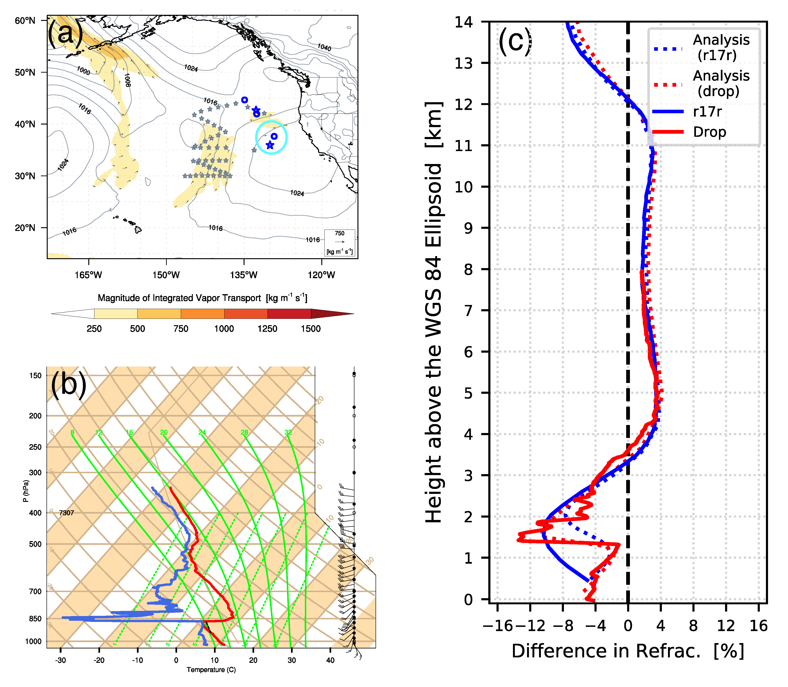
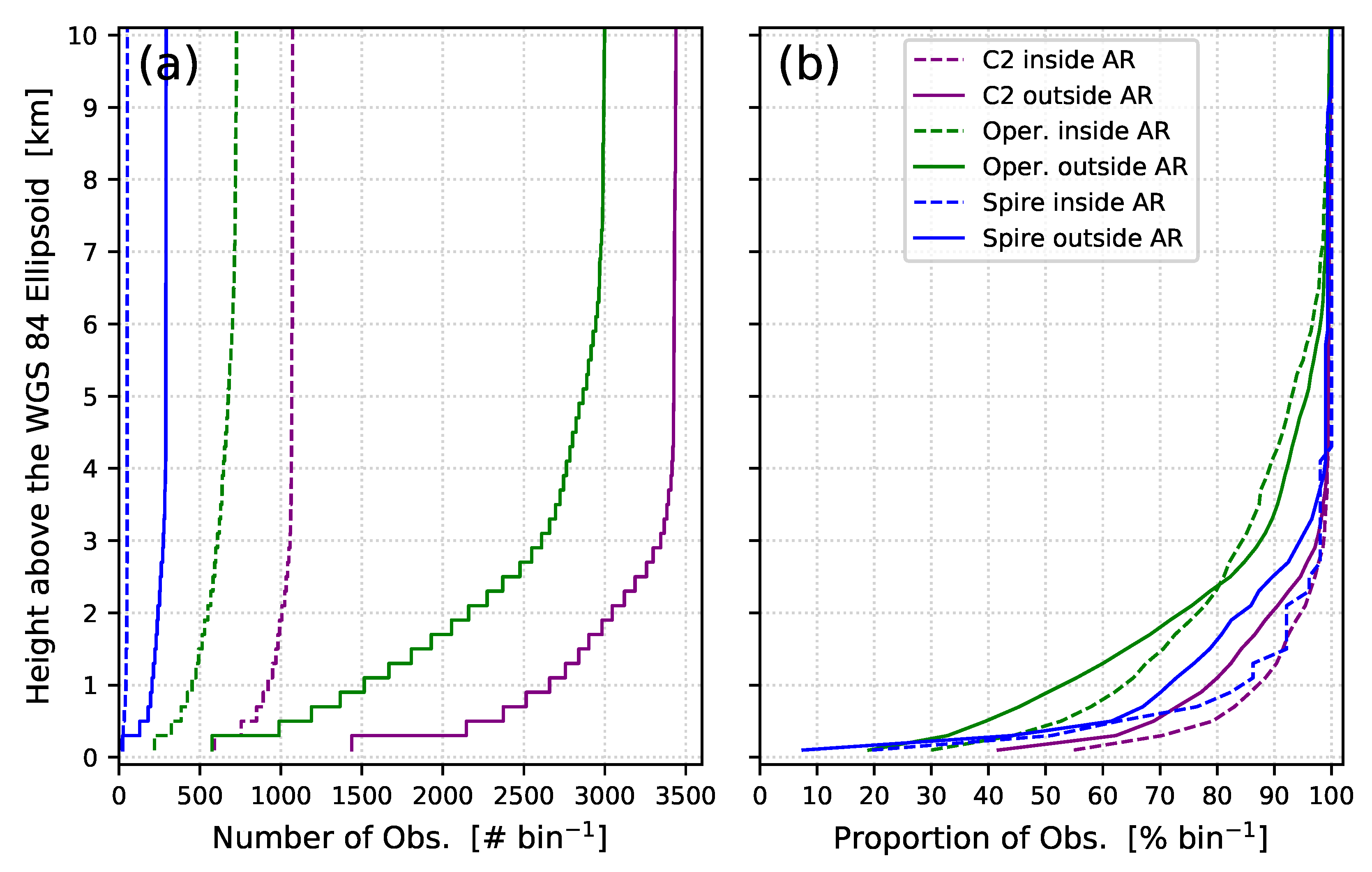
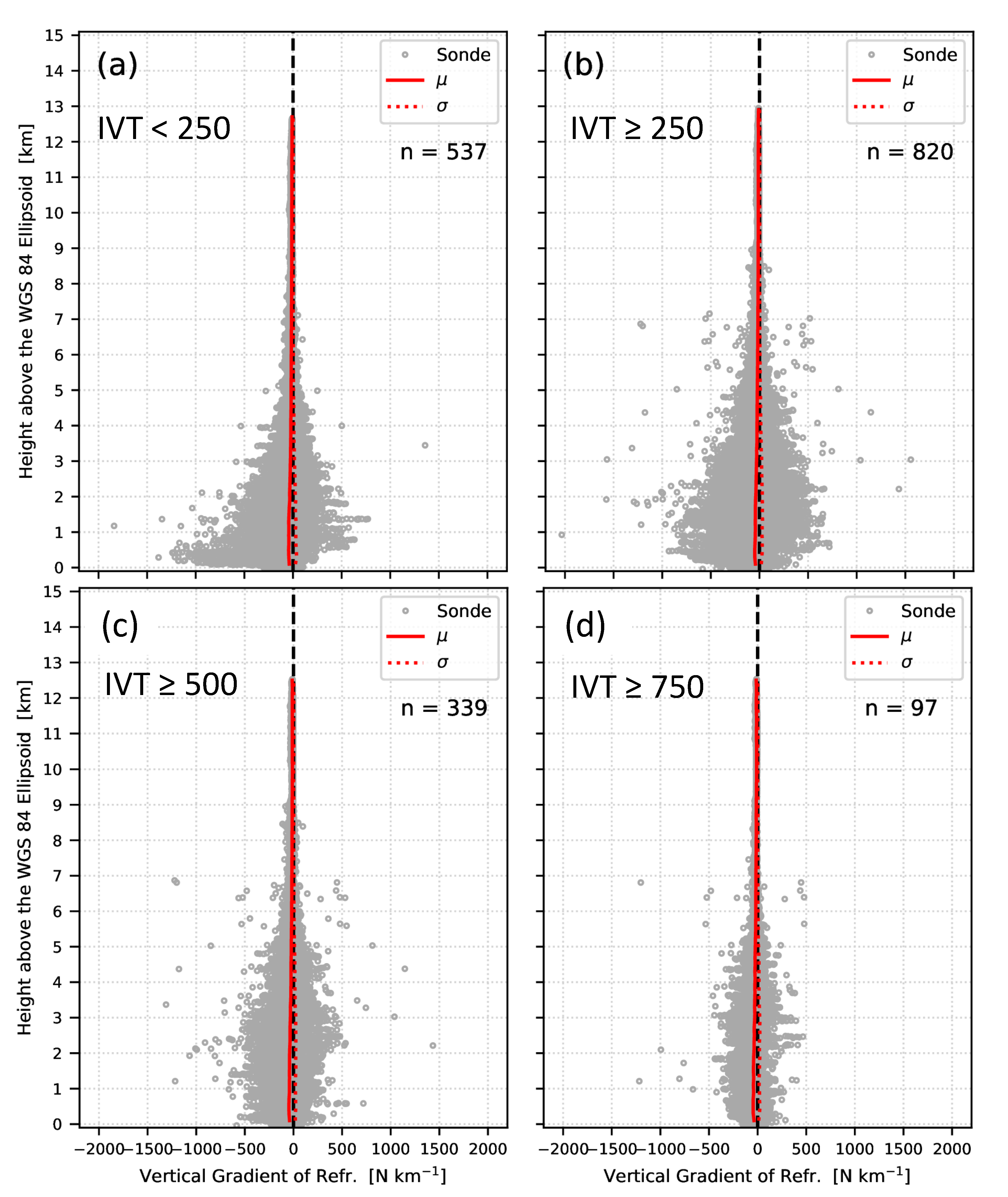
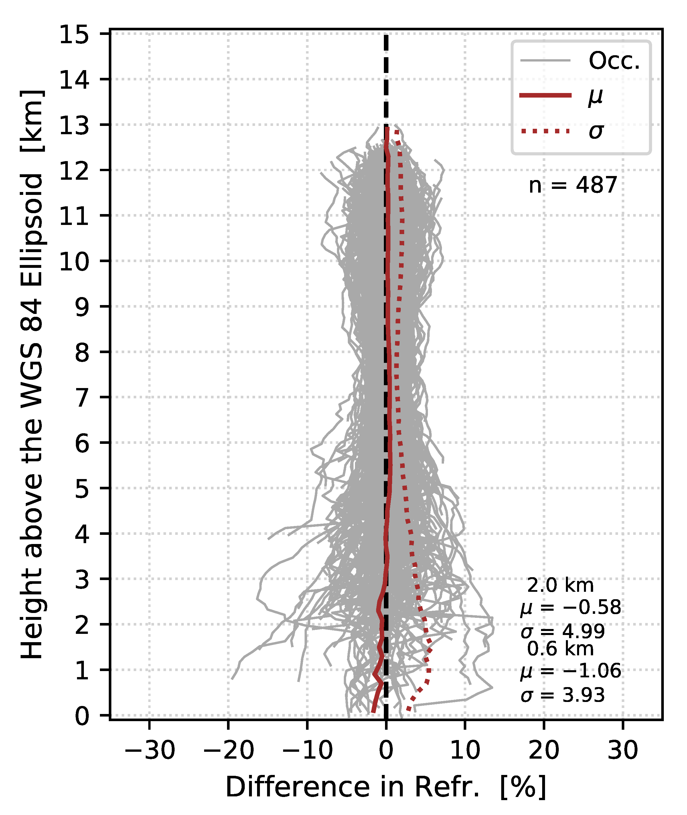
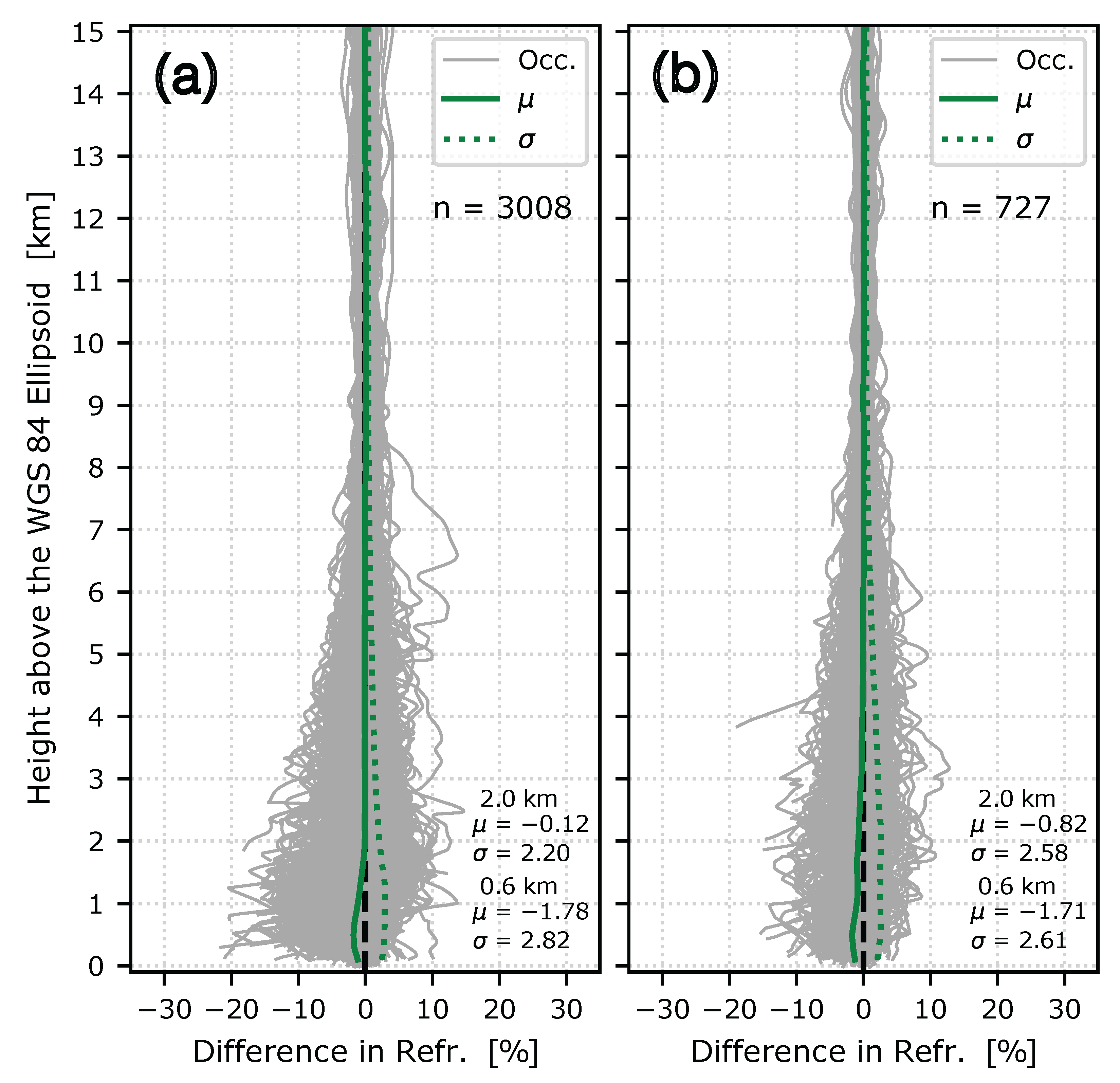
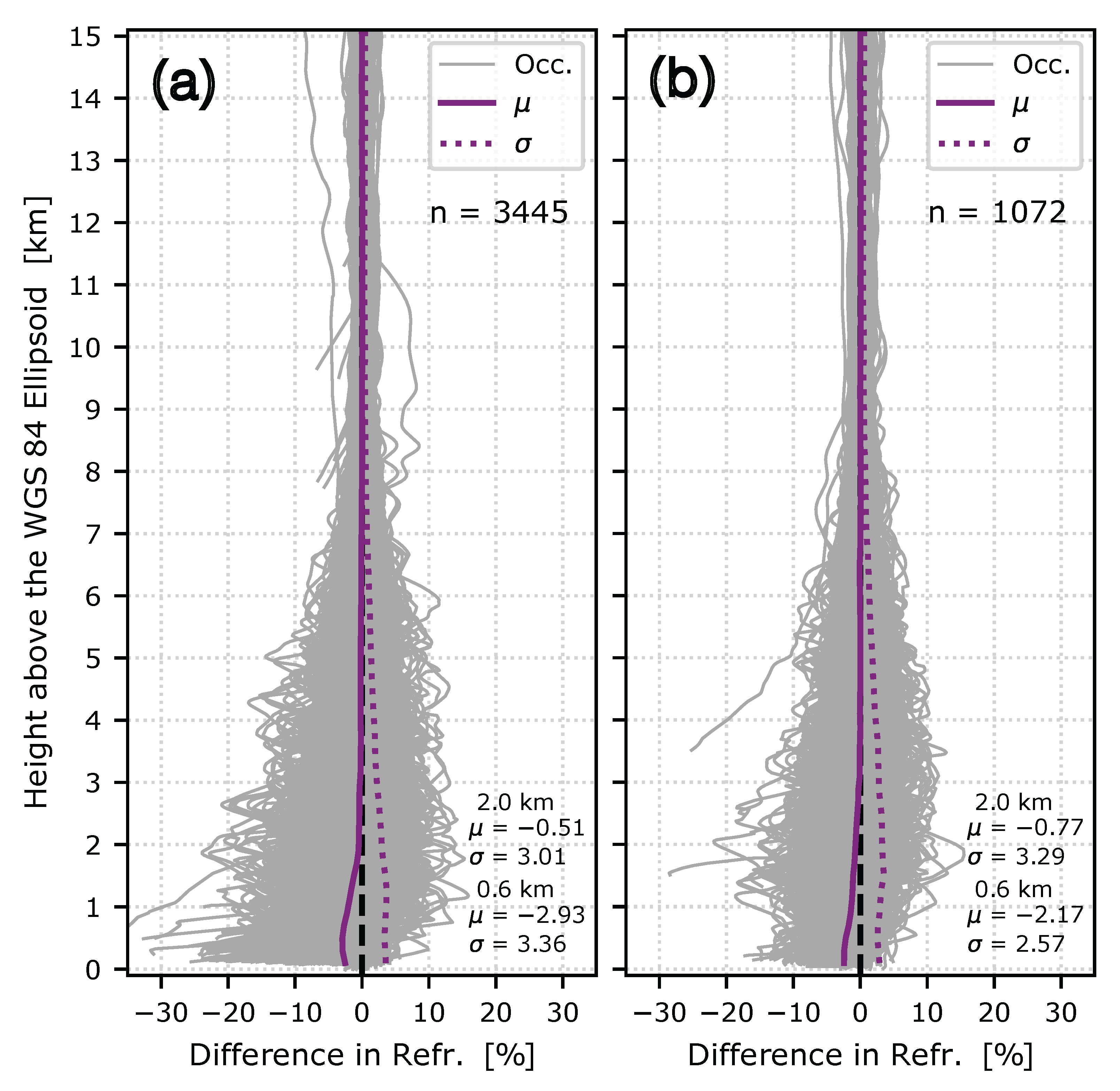
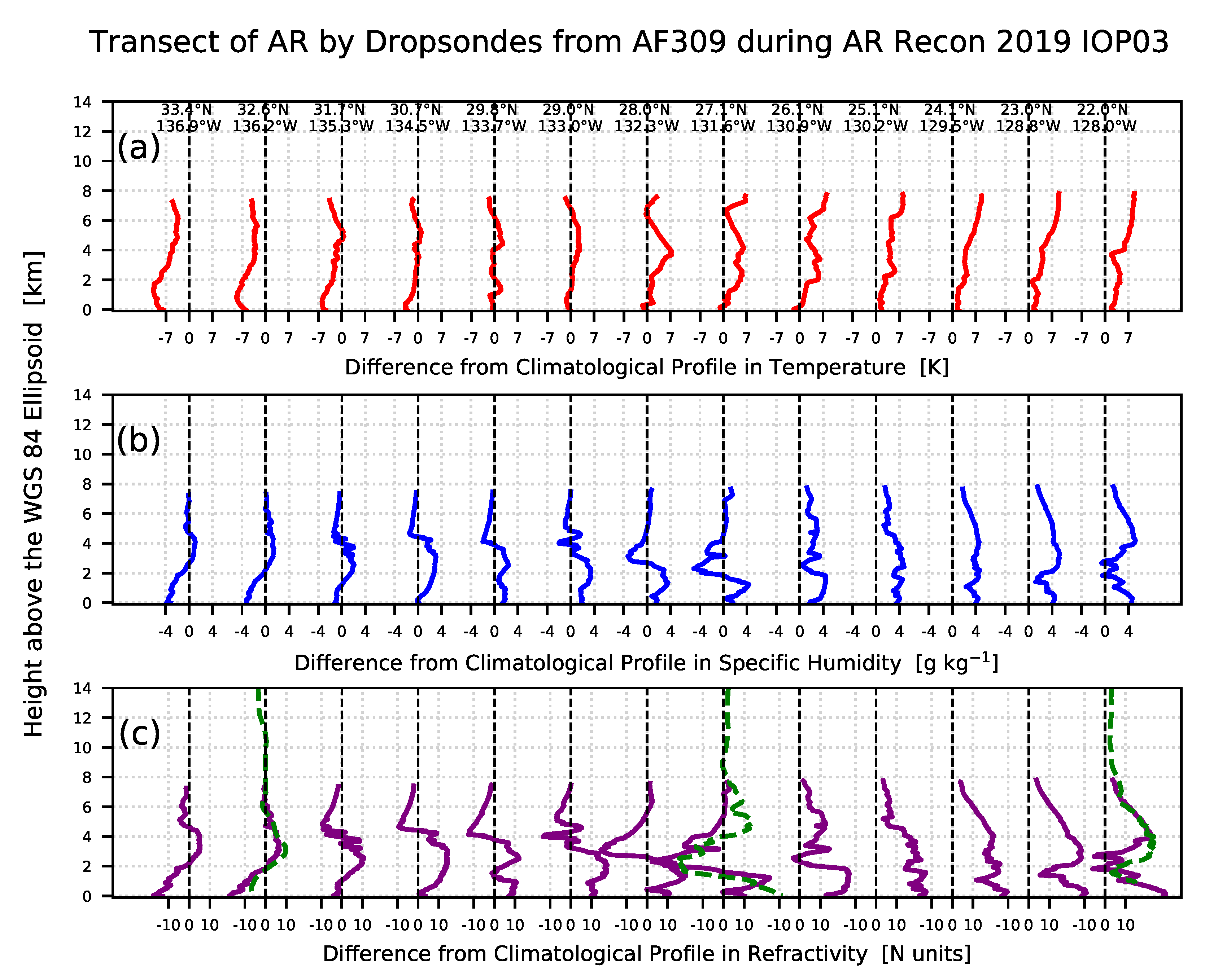
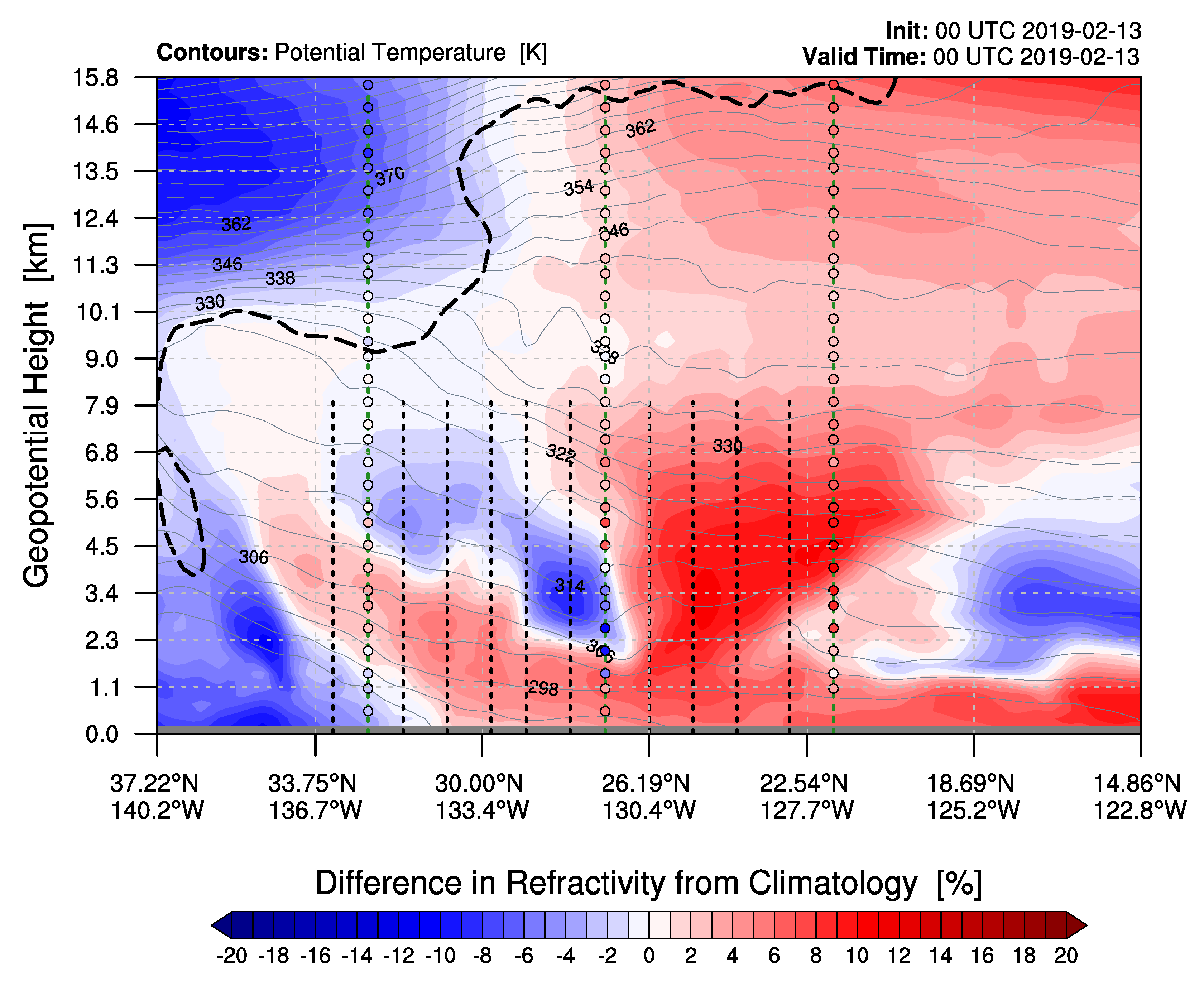
Table 1.
Observation sampling and density by dataset.
| Dataset | Samples (#) | IOPs (#) | Samples/IOP | Density/IOP (# deg) |
|---|---|---|---|---|
| Operational RO | 3735 | 29 | 128.8 | 0.037 |
| COSMIC-2 RO | 4517 | 17 | 265.7 | 0.076 |
| Spire RO | 342 | 6 | 57.0 | 0.016 |
| Combined | 8594 | 29 | 296.3 | 0.085 |
Table 2.
Observation sampling and density within an AR.
| Dataset | Samples (#) | IOPs (#) | Samples/IOP | Density/IOP (# deg) |
|---|---|---|---|---|
| Operational RO | 727 | 29 | 25.1 | 0.007 |
| COSMIC-2 RO | 1072 | 17 | 63.1 | 0.018 |
| Spire RO | 51 | 6 | 8.5 | 0.002 |
| Combined | 1850 | 29 | 63.8 | 0.018 |
Publisher’s Note: MDPI stays neutral with regard to jurisdictional claims in published maps and institutional affiliations. |
© 2022 by the authors. Licensee MDPI, Basel, Switzerland. This article is an open access article distributed under the terms and conditions of the Creative Commons Attribution (CC BY) license (https://creativecommons.org/licenses/by/4.0/).
Share and Cite
MDPI and ACS Style
Murphy, M.J., Jr.; Haase, J.S. Evaluation of GNSS Radio Occultation Profiles in the Vicinity of Atmospheric Rivers. Atmosphere 2022, 13, 1495. https://0-doi-org.brum.beds.ac.uk/10.3390/atmos13091495
AMA Style
Murphy MJ Jr., Haase JS. Evaluation of GNSS Radio Occultation Profiles in the Vicinity of Atmospheric Rivers. Atmosphere. 2022; 13(9):1495. https://0-doi-org.brum.beds.ac.uk/10.3390/atmos13091495
Chicago/Turabian StyleMurphy, Michael J., Jr., and Jennifer S. Haase. 2022. "Evaluation of GNSS Radio Occultation Profiles in the Vicinity of Atmospheric Rivers" Atmosphere 13, no. 9: 1495. https://0-doi-org.brum.beds.ac.uk/10.3390/atmos13091495
Note that from the first issue of 2016, this journal uses article numbers instead of page numbers. See further details here.