The Use of Multilayer Perceptrons to Model PM_2.5 Concentrations at Air Monitoring Stations in Poland

Abstract

The biggest problem facing air protection in Poland is the high levels of suspended particular matter concentrations. Air monitoring reports show that air quality standards, related to PM₁₀ and PM_2.5 concentrations, are exceeded every year in many Polish cities. The PM_2.5 aerosol fraction is particularly dangerous to human and animal health. Therefore, monitoring the level of PM_2.5 concentration should be considered particularly important. Unfortunately, most monitoring stations in Poland do not measure this dust fraction. However, almost all stations are equipped with analyzers measuring PM₁₀ concentrations. PM_2.5 is a fine fraction of PM₁₀, and there is a strong correlation between the concentrations of these two types of suspended dust. This relationship can be used to determine the concentration of PM_2.5. The main purpose of this analysis was to assess the accuracy of PM_2.5 concentration prediction using PM₁₀ concentrations. The analysis was carried out on the basis of long-term hourly data recorded at several monitoring stations in Poland. Artificial neural networks in the form of a multilayer perceptron were used to model PM_2.5 concentrations.

1. Introduction

Air pollution is considered as one of the main factors affecting the human population and the environment. Air pollution may cause various reactions in organisms, including mental health disorders [1,2]. It can cause negative changes in the human respiratory and circulatory systems, even when concentrations do not exceed permissible levels [3,4,5,6,7,8]. It was found that air pollution can negatively affect the economy [9,10,11,12]. Air pollution can also reduce crop yields in agriculture [13,14].

It should be highlighted that in many European countries, the levels of particulate matter (PM₁₀), NO₂, O₃, and benzo(a)pyrene (B(a)P) concentrations still exceed the permissible limits [15]. The World Health Organization estimates that many millions of people die prematurely due to poor air quality [16]. Once the pollutants are emitted into the air, it is impossible to stop them. If the pollutants enter the atmosphere, they contribute to the deterioration of air quality in the emission vicinity, and by spreading, they can have negative effects hundreds and thousands of kilometers from the point of emission. Therefore, air pollution is treated as a global threat, and emission reduction strategies are implemented in many countries. The control and reduction of anthropogenic emissions are now recognized as keys to good global air quality in the future.

The main gaseous pollutants are O₃, SO₂, NO_x, CO, and volatile organic compounds (VOCs). Atmospheric air is a multiphase system. The gas phase is the dominant phase, but there are also dispersed solid and liquid particles in the air, i.e., aerosols. Small aerosols can remain suspended in the air for long periods [17]. Therefore, to assess air quality, not only should the concentration of toxic gases be tested, but also the content of toxic compounds in the suspended aerosols, labelled as PM₁₀. PM₁₀ aerosols adsorb particularly dangerous contaminants, such as PAHs and heavy metals, on their surface. Similar to the EU, routine air pollution monitoring in Poland includes examination of the levels of benzo(a)pyrene and four heavy metals (Pb, Cr, Ni, and Cd) in PM₁₀ particles [18]. In recent years, air monitoring systems have been introducing the measurement of a finer fraction of particulate matter, of particle sizes not exceeding 2.5 µm, called PM_2.5. The impacts attributable to exposure to PM_2.5 in Europe have been presented in annual reports. These assessments are based on two different mortality endpoints: premature death and years of life lost (YLL) [19]. In Poland, PM_2.5 concentrations constantly exceed the permissible limits and cause over 40,000 premature deaths annually [15].

The need to model air pollutant concentrations is usually associated with the problem of supplementing missing data in measurement sets from air monitoring stations [20,21,22,23]. The relationships between the measured pollutants’ concentrations are used for modeling. Meteorological parameters can also be useful, if available. The concentrations of primary pollutants are correlated because they come from the same emission sources, e.g., from fuel combustion processes. If the goal of modeling is to predict measurement gaps, regression techniques are typically used. In the past, multivariate regression models were built according to the procedures of classical statistics [24]. Currently, artificial intelligence methods are used more and more often, because they allow for a deeper exploration of knowledge hidden in measurement sets [25]. In this group of models, models using artificial neural networks (ANNs) are very popular [26,27,28,29,30,31,32,33,34]. With the rapid development of artificial intelligence, deep learning techniques are increasingly used in big data analytics to solve various classification and regression problems for air pollution prediction [25,35]. For example, deep learning models based on convolutional neural networks are useful for processing historical air pollution data with spatiotemporal correlations [36,37]. In recent years, various variants of recurrent neural networks (RNNs) have been intensively developed, such as the original recurrent neural networks (original RNN), gated recurrent units (GRUs), long short-term memory (LSTM), read-first LSTM (RLSTM), and long short-term memory neural network extended (LSTME) [25]. These types of neural networks allow us to extract temporal correlation in raw data; therefore, they are often used to create forecasts.

The biggest problem facing air protection in Poland is the high suspended particular matter concentrations. The air monitoring reports show that air quality standards, related to PM₁₀ and PM_2.5 concentrations, are exceeded every year in many Polish cities [15,38]. The PM_2.5 aerosol fraction is particularly dangerous to human and animal health. Therefore, monitoring the level of PM_2.5 concentrations should be considered particularly important. Unfortunately, most monitoring stations in Poland do not measure this fraction of aerosol. However, almost all stations are equipped with analyzers measuring PM₁₀ concentrations. PM_2.5 is a fine fraction of PM₁₀, and there is a strong correlation between the concentrations of these two types of suspended dust [39,40]. This relationship can be used to determine the concentration of PM_2.5. The main purpose of this study was to assess the accuracy of PM_2.5 concentration prediction using PM₁₀ concentrations. The analysis was carried out on the basis of long-term hourly data recorded at several monitoring stations in Poland. Artificial neural networks in the form of a multilayer perceptron were used to model hourly PM_2.5 concentrations.

2. Materials and Methods

2.1. Air Monitoring Stations

Data from 6 automatic air monitoring stations located in Poland from the cities of Jelenia Gora, Lublin, Plock, Radom, Kedzierzyn-Kozle, and Olsztyn were used in the study. The criterion for selecting the stations was the availability of the results of measuring the concentrations of basic air pollutants, including PM₁₀ and PM_2.5. At the six selected stations, concentrations of PM₁₀, PM_2.5, O₃, SO₂, NO_x, and CO were recorded throughout or almost throughout the 2015–2021 measurement period.

The locations of the stations are shown in Figure 1. The stations were managed by the Chief Inspectorate of Environmental Protection in Poland. All selected stations were the background type, located in urban areas.

Table 1. Basic information about the air monitoring stations [41].

Air Monitoring Station	Address	International Code	Geographical Coordinates, WGS84	Station Type	Area Type
Jelenia Gora	6 Oginskiego Str.	PL0585A	Φ 50.913433 λ 15.765608	background	city
Lublin	13. Obywatelska Str.	PL0507A	Φ 51.259431 λ 22.569133	background	city
Plock	28 Mikolaja Reja Str.	PL0136A	Φ 52.550938 λ 19.709791	background	city
Radom	1 Tochtermana Str.	PL0138A	Φ 51.399084 λ 21.147474	background	city
Kedzierzyn-Kozle	5 Boleslawa Smialego Str.	PL0218A	Φ 50.349608 λ 18.236575	background	city
Olsztyn	16 Puszkina Str.	PL0175A	Φ 53.789233 λ 20.486075	background	city

contains the basic information about the air monitoring stations.

2.2. Air Monitoring Data

In this study, hourly values of CO, SO₂, PM₁₀, PM_2.5, O₃, and NO_x concentrations, recorded in the years 2015–2021, were used. The data were provided by the Chief Inspectorate of Environmental Protection in Poland. The air monitoring data were officially validated data. We selected stations where both PM₁₀ and PM_2.5 concentration measurements were obtained in the period 2015–2021.

The following symbols were used to describe the time series (variables): D, numeric day; H, numeric hour; CO, hourly average of CO concentration (mg/m³); SO₂, hourly average of SO₂ concentration (µg/m³); PM₁₀, hourly average of PM₁₀ concentration (µg/m³); PM_2.5, hourly average of PM_2.5 concentration (µg/m³); O₃, hourly average of O₃ concentration (µg/m³); and NO_x, hourly average of NO_x concentration (µg/m³).

2.3. Temporal Variables’ Transformation

The date in numerical form was prepared to replace the date with a value ranging from 0 to 1. For the first day of the year (1 January), a value of 1 was assumed, and for the middle date of the year (2 July), a value of 0. In the first half of the year, the numeric date value decreased proportionally from 1 to 0. In the second half of the year, the numeric date value increased proportionally from 0 to 1.

The hour was also converted to a numerical value ranging from 0 to 1. For midnight (24.00), a value of 0 was assumed, and for the middle of the day (12.00), a value of 1. In the first half of the day, the numerical hour value proportionally increased from 0 to 1. In the second half of the day, the numerical hour value proportionally decreased from 1 to 0.

2.4. Data Preparation

Only those annual measurement series whose completeness exceeded 85% were included in the analysis. If this condition was not met, data from the entire year were removed so that the analyzed data evenly covered all seasons of the calendar year. Cases with incomplete measurements were removed from the data set. A few cases where the registered concentrations of pollutants had negative values were also removed. Only cases for which all measured concentration values were present in a given measurement hour were selected for further analysis.

Table 2. Completeness of the time series after removing cases with missing data, 2015–2021.

		Completeness of the Annual Series
Air Monitoring Station	Total Number of Observations (Cases)	2015 %	2016 %	2017 %	2018 %	2019 %	2020 %	2021 %	2015–2021 1 %
Jelenia Gora	56,362	85.1	90.9	86.8	94.6	93.6	95.6	96.2	91.8
Lublin	39,336	-	-	88.9	91.7	88.4	92.5	87.2	89.8
Plock	51,169	-	98.6	99.2	90.9	98.8	98.4	97.7	97.3
Radom	57,568	92.1	89.3	96.1	97.6	95.8	98.0	87.8	93.8
Kedzierzyn-Kozle	23,838	-	88.9	-	90.8	-	-	92.1	90.6
Olsztyn	41,126	-	-	87.2	91.5	96.7	96.3	97.5	93.8

¹ The completeness of the series was assessed only for the years covered by the analysis.

shows the completeness of time series for individual monitoring stations after removing cases with missing data.

Table 3. Statistical description of measured variables at the air monitoring stations, 2015–2021.

Air Monitoring Station	Statistical Parameter	CO mg/m3	SO2 µg/m3	PM10 µg/m3	PM2.5 µg/m3	O3 µg/m3	NOx µg/m3
Jelenia Gora	Minimum value	0.012	0.0	0.1	0.1	0.0	0.0
	Maximum value	4.169	83.3	407.7	375.9	194.3	426.3
	Mean	0.399	5.0	26.8	21.0	52.8	15.9
	Standard deviation (SD)	0.275	4.6	28.8	26.6	33.4	17.7
Lublin	Minimum value	0.000	0.0	0.3	0.2	0.0	0.0
	Maximum value	5.323	56.9	496.0	438.0	176.1	766.7
	Mean	0.354	4.8	28.7	21.7	45.7	29.7
	Standard deviation (SD)	0.276	3.1	23.6	20.8	27.7	34.6
Plock	Minimum value	0.110	0.0	0.7	0.1	0.3	0.3
	Maximum value	3.313	322.8	346.9	167.6	177.3	838.1
	Mean	0.354	3.6	27.0	18.9	49.3	20.1
	Standard deviation (SD)	0.160	6.6	18.7	15.1	25.8	22.0
Radom	Minimum value	0.090	0.0	1.2	0.1	0.1	0.8
	Maximum value	6.246	76.4	449.3	302.3	174.3	947.8
	Mean	0.418	3.0	32.6	23.7	46.0	31.6
	Standard deviation (SD)	0.269	3.8	25.9	21.2	27.7	34.5
Kedzierzyn -Kozle	Minimum value	0.064	0.2	0.8	0.2	0.0	0.4
	Maximum value	2.561	56.1	296.5	264.1	175.2	389.0
	Mean	0.387	6.2	32.3	24.5	45.7	23.5
	Standard deviation (SD)	0.248	4.7	26.6	23.5	32.1	24.3
Olsztyn	Minimum value	0.061	0.0	0.7	0.5	0.0	0.0
	Maximum value	3.102	55.7	251.0	138.4	144.0	411.3
	Mean	0.332	4.5	21.4	15.9	48.9	17.8
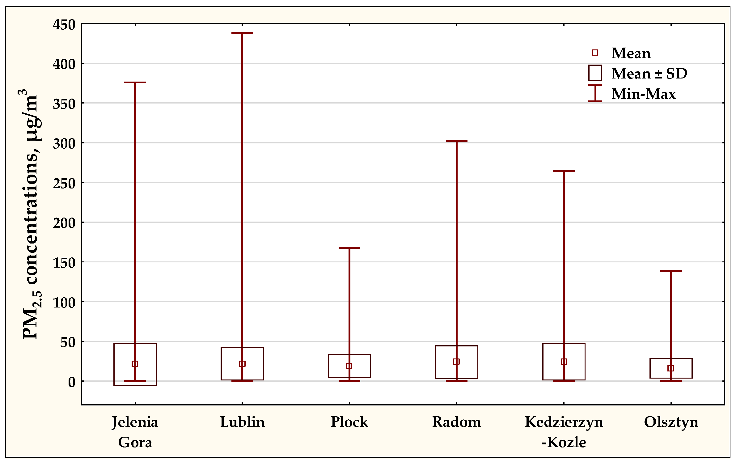
	Standard deviation (SD)	0.156	3.2	15.9	12.7	25.7	21.1

presents a statistical description of the concentrations measured at individual air monitoring stations, only for complete cases. Among the selected stations, the highest maximum concentrations of particulate matter PM_2.5 occurred at the measuring stations in Lublin, Jelenia Gora, Radom, and Kedzierzyn-Kozle, while the lowest occurred in Plock and Olsztyn.

Figure 2 shows the variability in PM_2.5 concentration at the considered air monitoring stations.

2.5. Regression Models (Design)

Modeling was carried out using the module Artificial Neural Networks in the STATISTICA program, version 13.3, TIBCO Software Inc., Palo Alto, CA, USA. The multilayer perceptron (MLP) architecture was used to create the regression models. It was assumed that each multilayer perceptron consisted of 10 neurons in one hidden layer. During network initialization, the data set was randomly divided into three subsets: the training (50% of cases), validation (25% of cases), and test (25% of cases) subsets. The classification of cases did not change in the network learning process. The number of all cases in the sets is given in Table 2 as the total number of observations. The Broyden–Fletcher–Goldfarb–Shanno (BFGS) algorithm was used in the learning process. This algorithm is dedicated to numerical optimization [42]. The mathematical foundations of the algorithm were formulated by mathematicians in 1970 [43,44,45,46].

In order to avoid overfitting during the training of the network, in addition to the training set, a test set was used, in accordance with the validation procedure implemented in STATISTICA Automatic Neural Networks [47]. Test data were used to evaluate the progress of the network as the network was trained. The neural network was optimized in relation to the training data during the learning process. Stopping the network training process early enough prevented overfitting and maximized the degree of generalization. In each successive cycle, the applied early stopping technique carried out the learning process in accordance with the following procedure [47]:

• Feed the network data from the training data set.
• Calculate the prediction (network outputs).
• Calculate of the difference between the predicted and actual values of the output according to the data, using the error function.
• Repeat steps 1 and 2 until all input—output pairs from the training data set are exhausted.
• Use a learning algorithm to correct the neuron weights to obtain a smaller prediction error.
• Input all cases from the test data to the network input, obtain the prediction, compare it with the appropriate values of the data outputs, and calculate the network error.
• Compare the network error received with the error received in the previous cycle. If the error decreased, learning is continued in the next cycle, otherwise the process was stopped.

The validation data were not used in the network learning process. The network error was calculated for these data after training was complete. If the validation error did not significantly differ from the test error, then it was considered that the network generalized the data structure well.

STATISTICA Automatic Neural Networks scaled the input and output variables using a linear transformation according to extreme values in the data, so that all values fall within the range (0,1).

The learning process was limited to 300 epochs. The activation function in the hidden neurons was logistic, but this function for the output was linear. The single output (PM_2.5) of each MLP model was taken from the same time step as the predictors. The network was randomly initiated using the Gaussian method. The initial weights were normally distributed with a mean of 0 and a variance of 1. The sum of squares (SOS) was assumed as the error function. SOS was the sum of the squared distances between predicted and actual values. Each prediction was made 5 times, each time with different randomly selected initial weights and with a different division of cases into subsets. The most accurate of the 5 created models was selected for the study. The other models were rejected. Accuracies of models were assessed by calculating the MEA and RMSE together for the cases from the three subsets (training, test, and validation). The created networks slightly differed in the modeling error. They had the same structure, but differed in terms of input and output weights of individual neurons.

Regression models were created for each monitoring station, in which the PM_2.5 concentration was the output (explained variable), while the input data (explanatory variables) were entered in the following variants:

I.

D, H → (MLP 2-10-1, Figure 3a);

II.

D, H, PM₁₀ → (MLP 3-10-1, Figure 3b);

III.

D, H, PM₁₀, CO → (MLP 4-10-1, Figure 3c);

IV.

D, H, PM₁₀, CO, SO₂, O₃, NO_x → (MLP 7-10-1, Figure 3d).

Figure 3 shows the architecture diagrams of a multilayer perceptron with 10 neurons in one hidden layer for subsequent variants of the explanatory variables.

Figure 3. Architecture diagrams of the multilayer perceptrons with ten neurons in a single hidden layer. The diagrams for various variants of explanatory variables: (a) D, H; (b) D, H, PM₁₀; (c) D, H, PM₁₀, CO; (d) D, H, PM₁₀, CO, SO₂, O₃, NO_x.

Figure 3. Architecture diagrams of the multilayer perceptrons with ten neurons in a single hidden layer. The diagrams for various variants of explanatory variables: (a) D, H; (b) D, H, PM₁₀; (c) D, H, PM₁₀, CO; (d) D, H, PM₁₀, CO, SO₂, O₃, NO_x.

For comparison, using the linear regression method of least squares, PM_2.5 concentration was modeled for the variant with only one predictor—PM₁₀. The Multiple Regression module in the STATISTICA TIBCO Software Inc program was used for modeling. The results were models called LINEAR.

2.6. Assessment of the Approximation Error

The mean absolute error (MAE) and root mean squared error (RMSE) values, which were calculated on the basis of the discrepancies between the actual and predicted values, were used to assess the accuracy of the regression models obtained. The formulas for calculating individual errors are shown in Equations (1) and (2).

MAE:

$$\mathrm{MAE}=\frac{1}{\mathrm{n}}{\displaystyle \sum }_{\mathrm{i}=1}^{\mathrm{n}}\left|{\mathrm{x}}_{\mathrm{i}}-{\mathrm{y}}_{\mathrm{i}}\right|$$

(1)

RMSE:

$$\mathrm{RMSE}=\sqrt{\frac{{{\displaystyle \sum }}_{\mathrm{i}=1}^{\mathrm{n}}{\left({\mathrm{x}}_{\mathrm{i}}-{\mathrm{y}}_{\mathrm{i}}\right)}^2}{\mathrm{n}}}$$

(2)

where n is the number of cases, y is the predicted concentrations, x is the real concentrations, and i is the case number.

2.7. Verification of Models

In order to verify the usefulness of the obtained MLP neural network models for modeling current concentrations of PM_2.5, trial modeling was carried out for several daily episodes from 2022. The MLP 7-10-1 and MLP 3-10-1 models trained on historical data (2015–2021) from the considered air monitoring station were used for prediction. Trial modeling was performed to answer the question of whether it is possible to use neural networks trained on historical data to model PM_2.5 concentration in a later measurement period.

In order to assess the quality of prediction in extreme conditions, the modeling error was calculated for selected cases of very low (≤1.0 µg/m³) and very high (≥100.0 µg/m³) PM_2.5 concentrations. In addition, the universality of the obtained neural models was verified by using one of the trained networks to model PM_2.5 concentrations at other air monitoring stations.

3. Results

3.1. Annual and Diurnal Courses of PM_2.5 and PM₁₀ Concentrations

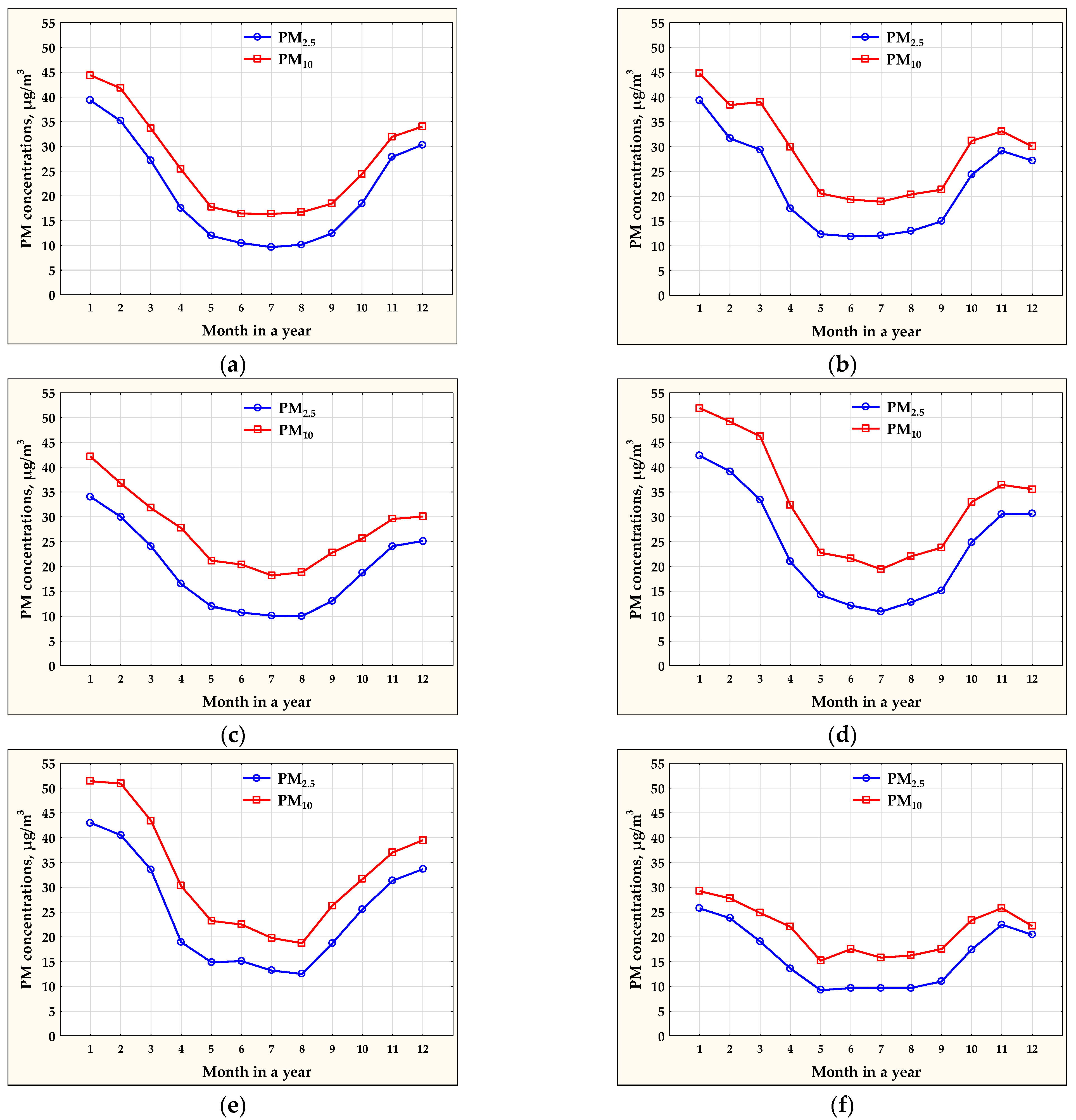
Based on the time series used in the analysis, statistical courses of PM_2.5 and PM₁₀ concentrations in the annual cycle were calculated for each air monitoring station. The results were shown in Figure 4. The courses indicated that the lowest concentrations of suspended particulate matter appeared in May–September. In the typical winter months of January and February, concentrations of particulate matter reached the highest values.

Figure 5 shows the daily courses of PM₁₀ and PM_2.5 concentrations. The courses indicated that the lowest concentrations of suspended particulate matter appeared at noon and in the afternoon hours. In the evening and at night, the concentrations of particulate matter reached the highest values at all monitoring stations.

3.2. Preliminary Analysis of Correlations

A correlation analysis was performed for air pollutant concentrations at individual air monitoring stations. The analysis was performed to find the best predictors for PM_2.5 concentrations. The Pearson’s correlation coefficients were presented in the

Table 4. Pearson’s correlation coefficient for variables registered at the air monitoring stations, 2015–2021.

Air Monitoring Station		CO	SO2	PM10	PM2.5	O3	NOx
Jelenia Gora	CO	1.000
	SO2	0.669	1.000
	PM10	0.902	0.668	1.000
	PM2.5	0.926	0.682	0.978	1.000
	O3	−0.484	−0.258	−0.375	−0.434	1.000
	NOx	0.743	0.570	0.711	0.708	−0.516	1.000
Lublin	CO	1.000
	SO2	0.326	1.000
	PM10	0.772	0.398	1.000
	PM2.5	0.788	0.404	0.947	1.000
	O3	−0.446	−0.145	−0.325	−0.440	1.000
	NOx	0.750	0.220	0.585	0.547	−0.434	1.000
Plock	CO	1.000
	SO2	0.118	1.000
	PM10	0.768	0.145	1.000
	PM2.5	0.827	0.148	0.923	1.000
	O3	−0.520	0.000	−0.361	−0.501	1.000
	NOx	0.738	0.083	0.497	0.483	−0.424	1.000
Radom	CO	1.000
	SO2	0.546	1.000
	PM10	0.863	0.636	1.000
	PM2.5	0.885	0.652	0.945	1.000
	O3	−0.485	−0.213	−0.431	−0.512	1.000
	NOx	0.809	0.354	0.664	0.631	−0.455	1.000
Kedzierzyn-Kozle	CO	1.000
	SO2	0.503	1.000
	PM10	0.818	0.534	1.000
	PM2.5	0.839	0.529	0.967	1.000
	O3	−0.531	−0.152	−0.406	−0.463	1.000
	NOx	0.711	0.309	0.621	0.608	−0.548	1.000
Olsztyn	CO	1.000
	SO2	0.141	1.000
	PM10	0.641	0.202	1.000
	PM2.5	0.759	0.197	0.895	1.000
	O3	−0.581	−0.071	−0.295	−0.479	1.000
	NOx	0.744	0.141	0.565	0.561	−0.522	1.000

. For all the analyzed stations, the highest correlation coefficient in relation to PM_2.5 concentration occurred for PM₁₀ concentration, which was slightly lower for CO concentration. These two predictors were used to create models in variants II and III (see Section 2.5). Because all concentration variables had relatively high coefficients in relation to PM_2.5, in the full-dimensional variant, in addition to time variables, all concentration variables were used (variant IV in Section 2.5.).

3.3. Results of Modeling PM_2.5 Concentrations

For each variant of model, for individual air monitoring stations, modeling errors of the PM_2.5 concentration were separately calculated in relation to the actual PM_2.5 concentration. To assess the modeling accuracy, two error measures were calculated: MAE and RMSE. A brief description of the models and the values of the prediction errors obtained for them was presented in

Table 5. Values of approximation errors of PM_2.5 concentrations in MLP models for 4 variants with different numbers of predictors. For comparison, the results for linear regression models, called LINEAR, were added.

Air Monitoring Station	Regression Model	Explanatory Variable (Predictors)	MAE µg/m3	RMSE µg/m3
Jelenia Gora	LINEAR	PM10	3.92	5.53
	MLP 2-10-1	D, H,	13.94	24.19
	MLP 3-10-1	D, H, PM10,	3.25	4.72
	MLP 4-10-1	D, H, PM10, CO	2.99	4.18
	MLP 7-10-1	D, H, PM10, CO, SO2, O3, NOx	2.91	4.09
Lublin	LINEAR	PM10	4.68	6.69
	MLP 2-10-1	D, H,	11.90	20.12
	MLP 3-10-1	D, H, PM10,	4.04	5.88
	MLP 4-10-1	D, H, PM10, CO	4.01	5.74
	MLP 7-10-1	D, H, PM10, CO, SO2, O3, NOx	3.61	5.30
Plock	LINEAR	PM10	3.70	5.78
	MLP 2-10-1	D, H,	8.67	12.88
	MLP 3-10-1	D, H, PM10,	2.68	4.06
	MLP 4-10-1	D, H, PM10, CO	2.46	3.66
	MLP 7-10-1	D, H, PM10, CO, SO2, O3, NOx	2.23	3.36
Radom	LINEAR	PM10	4.40	6.94
	MLP 2-10-1	D, H,	11.23	18.10
	MLP 3-10-1	D, H, PM10,	3.36	5.68
	MLP 4-10-1	D, H, PM10, CO	3.16	5.01
	MLP 7-10-1	D, H, PM10, CO, SO2, O3, NOx	2.80	4.39
Kedzierzyn-Kozle	LINEAR	PM10	4.04	5.98
	MLP 2-10-1	D, H,	13.66	21.05
	MLP 3-10-1	D, H, PM10,	3.68	5.51
	MLP 4-10-1	D, H, PM10, CO	3.60	5.30
	MLP 7-10-1	D, H, PM10, CO, SO2, O3, NOx	3.22	4.73
Olsztyn	LINEAR	PM10	3.42	5.66
	MLP 2-10-1	D, H,	7.76	11.21
	MLP 3-10-1	D, H, PM10,	2.04	3.29
	MLP 4-10-1	D, H, PM10, CO	2.00	3.21
	MLP 7-10-1	D, H, PM10, CO, SO2, O3, NOx	1.78	2.88

. MAE and RMSE error values for the neural models were also graphically presented in Figure 6.

For comparison, the results of the linear regression models, called LINEAR, were added. The correlation between PM₁₀ and PM_2.5 concentrations was so strong that simple linear models exploring only the PM₁₀ concentration provided reasonable prediction accuracy. Using nonlinear neural models, the modeling error could be significantly reduced.

For all stations, exceptionally large prediction errors were obtained for the simplest neural models (variant I), in which the predictors were only time variables D and H. A very significant increase in modeling quality was observed for models in variant II, in which one of the predictors was the PM₁₀ variable. PM₁₀ emerged as the most important explanatory variable. The addition of CO concentration variable to the model inputs (MLP 4-10-1 models) resulted in a few percent improvement in the accuracy of the approximation. Including all available concentration variables in the model inputs (MLP 7-10-1 variants) reduced the modeling error to a slight extent.

Scatterplots were used to compare the modeled and observed values of PM_2.5 concentrations at individual automatic air monitoring stations (Figure 7). The results were shown for the most accurate models, with seven explanatory variables (variant IV: MLP 7-10-1). The scatterplots also showed perfect fit lines (blue lines: y = x) and regression lines (red lines). Linear regression equations and determination coefficients were also calculated.

3.4. Verification of Models

To evaluate the quality of prediction in extreme conditions, the modeling error was calculated for selected cases of very low (≤1.0 µg/m³) and very high (≥100.0 µg/m³) PM_2.5 concentrations. The results were presented in

Table 6. Modeling errors and some statistics in the extreme low and high ranges of PM_2.5 concentrations at different air monitoring stations (variant MLP 7-10-1).

Air Monitoring Station	Extreme Concentration Threshold	Number of Cases	PM2.5/PM10 Ratio %	MAE µg/m3	RMSE µg/m3
Jelenia Gora	≤1.0	314	34.2	3.81	4.39
	≥100.0	1346	91.6	6.35	7.97
Lublin	≤1.0	55	25.2	4.64	5.12
	≥100.0	440	89.6	8.41	11.65
Plock	≤1.0	46	30.5	2.15	2.17
	≥100.0	155	80.6	6.33	8.54
Radom	≤1.0	33	18.7	1.94	1.98
	≥100.0	729	84.9	12.47	15.92
Kedzierzyn-Kozle	≤1.0	48	30.9	3.53	3.89
	≥100.0	428	88.8	8.11	10.23
Olsztyn	≤1.0	14	63.2	1.32	2.51
	≥100.0	24	90.0	10.88	14.13

. The modeling errors calculated for extremely high PM_2.5 concentrations were always much higher than those calculated for the full range of concentrations. This effect can be explained by the specifics of the neural network learning algorithm. Without preprocessing the input data, the model better fit the concentration levels it saw most often in the training process, i.e., the most common cases. Cases of extremely high concentrations were under-represented, and the fit of the model to them was worse. The situation was different in the range of the lowest concentrations. The MAE and RMSE values in modeling very low concentrations could be even lower than the values of these errors estimated for the entire range of concentrations. The effects described above were noted in other studies, in which errors of the same model were analyzed in different concentration ranges of the modeled pollutant. It was stated that the application of one neural network to the entire concentration range resulted in different prediction accuracies in various concentration subranges [33,34]. It was proven that the prediction quality can be improved if one neural network model is replaced with several models (submodels) adapted to specific concentration subranges [48]. It should be noted that the percentage share of PM_2.5 in PM₁₀, at extremely high concentrations of PM_2.5, was very high and exceeded 80% at all air monitoring stations.

In order to verify the usefulness of the obtained neural models for modeling the concentration of PM_2.5, three different daily episodes that occurred at various air monitoring stations in 2022 were selected. PM_2.5 concentration modeling was carried out using the models trained on historical data from the same air monitoring station. Models of the MLP 7-10-1 and MLP 3-10-1 types were used for modeling. Episodes with different levels of PM_2.5 concentrations were selected for the study: in Olsztyn on 26 July 2022, in Plock on 26 July 2022, and in Jelenia Gora on 12–13 November 2022.

Figure 8 shows the daily courses of the actual and modeled PM_2.5 concentrations for the chosen episodes. The values of RMSE were calculated for both variants of the models: MLP 7-10-1 and MLP 3-10-1. The obtained results of the modeling errors for the individual episodes were comparable to the errors obtained when training neural networks. For the measuring station in Olsztyn, the RMSE error of prediction with the MLP 7-10-1 model was even lower. During this episode, the RMSE value was 1.4 µg/m³, and during network training, it was 4.0 µg/m³. During the episode in Plock, the RMSE value for the MLP 7-10-1 model was 3.7 µg/m³, and during training of this network, it was 3.1 µg/m³. In the case of the episode at the station in Jelenia Gora, the modeling error was 3.6 µg/m³, while during network training, it was 3.9 µg/m³. The MLP 3-10-1 models proved to be less accurate than the MLP 7-10-1 models, but their accuracy should also be considered acceptable.

The results of the trials allowed us to confirm the usefulness of the considered models for the prediction of current PM_2.5 concentrations when the PM₁₀ concentrations are known.

The concept of building predictive models presented in this article has some limitations. Trained neural networks were addressed for specific air monitoring stations. Each of the generated models had its own specificity, but they were also partly universal. The universality of the obtained neural models was verified by using one of the trained networks to model PM_2.5 concentrations at other air monitoring stations. In order to predict PM_2.5 concentrations at the monitoring stations in Jelenia Gora, Lublin, Radom, Kedzierzyn-Kozle, and Olsztyn, a model trained on data from the monitoring station in Plock was used. The obtained approximation errors were presented in

Table 7. Approximation error values of PM_2.5 concentrations obtained using the neural network trained on data from Plock.

Air Monitoring Station	MAE µg/m3	RMSE µg/m3
Jelenia Gora	3.67	8.12
Lublin	4.36	7.94
Radom	3.16	5.62
Kedzierzyn-Kozle	4.08	7.15
Olsztyn	2.21	3.41

. Analyzing the error values, it can be concluded that the accuracy of prediction using the “borrowed” model was lower than that of models dedicated to specific monitoring stations. MAE and RMSE values for the borrowed models were not very high; they are comparable to analogous prediction errors of simpler models, such as LINEAR or MLP 3-10-1. Borrowed models could be used at stations where there are no historical PM_2.5 measurements.

4. Discussion and Conclusions

MLP modeling of PM_2.5 concentrations using only time variables D and H (variant I) was burdened with a large error and did not give satisfactory results. However, compared with the naïve mean model, this kind of model has some advantages. In a naïve model that takes the mean as the modeling result for each case, the RMSE value would be equivalent to the standard deviation value in the set of real PM_2.5 concentrations. For MLP 2-10-1 models, the RMSE values at individual stations ranged from 12.0 to 24.0 µg/m³, meanwhile, the standard deviations in the PM_2.5 concentration sets had higher values: from 13.6 to 26.4 µg/m³. The RMSE prediction error was always lower than the standard deviation. This means that by using time variables, we could generate a model that was more accurate than the mean model.

The introduction of the PM₁₀ concentration as an additional input in the MLP 3-10-1 models (variant II) significantly improved the modeling quality. The RMSE values for the models of this variant were in the range of 3.8–6.0 µg/m³. It should be emphasized that PM₁₀ concentrations were very strongly correlated with PM_2.5 concentrations (correlation coefficients ranged from 0.858 to 0.978). Expanding the models by adding successive predictors (variants III and IV) made it possible to slightly reduce the level of RMSE modeling error to the range of 3.1–5.4 µg/m³.

A summary of modeling errors RMSE and some statistics on PM_2.5 and PM₁₀ concentrations was presented in

Table 8. Summary of modeling results: modeling errors and statistics on PM_2.5 and PM₁₀ concentrations for different air monitoring stations.

Air Monitoring Station	PM10, µg/m3		PM2.5, µg/m3		PM2.5/PM10 Ratio, %	r-Pearson PM2.5/PM10	RMSE, µg/m3
	Mean	SD	Mean	SD			MLP 3-10-1	MLP 7-10-1
Jelenia Gora	26.8	28.8	21.0	26.6	73.7	0.978	4.72	4.09
Lublin	28.7	23.6	21.7	20.8	73.7	0.947	5.88	5.30
Plock	27.0	18.7	18.9	15.1	68.1	0.923	4.06	3.36
Radom	32.6	25.9	23.7	21.2	69.9	0.945	5.68	4.39
Kedzierzyn-Kozle	32.3	26.6	24.5	23.5	72.3	0.967	5.51	4.73
Olsztyn	21.4	15.9	15.9	12.7	74.6	0.895	3.29	2.88

. The answer to the question regarding what determines the modeling error is not obvious. The models were obtained, and the modeling errors were estimated for data sets from six different air monitoring stations in Poland. It is usually assumed that the correlations between the dependent variable and the predictors are crucial in regression models. This regularity was not unequivocally confirmed in the obtained results. At the station in Jelenia Gora, with the highest correlation coefficient between PM₁₀ and PM_2.5 concentrations (r = 0.978), the modeling error was not the lowest. At the station in Olsztyn, with the lowest correlation coefficient between PM₁₀ and PM_2.5 concentrations (r = 0.858), the modeling error was not the highest. Additionally, the comparison of mean and standard deviation values, as well as the share of the PM_2.5 concentration in the PM₁₀ concentration, did not lead to clear conclusions. It should be assumed that each of the listed factors may have a partial impact on the modeling quality, and none of them is the dominant factor.

The main purpose of this study was to evaluate the accuracy of PM_2.5 concentration prediction using PM₁₀ concentrations. Such a prediction method could be used to model PM_2.5 concentrations in situations where the actual measurement was not performed, e.g., during a failure of the PM_2.5 analyzer. The results of other measurements must be available, including, above all, the measurement of PM₁₀ concentration. We also found that a trained neural network for a specific air monitoring station could be used to predict PM_2.5 concentrations at another station. Such prediction was less accurate because it was burdened with an additional error resulting from the mismatch between the model and the station.

The most important conclusions that result from the conducted analysis are as follows:

• In order to obtain a low PM_2.5 prediction error using the MLP models, it is enough to use the date and time in numerical form and the PM₁₀ concentration as explanatory variables.
• Including more explanatory variables slightly increases the accuracy of the MLP regression model.
• Neural regression models trained on archival data can be successfully used to model current PM_2.5 concentrations.
• The level of prediction error may be influenced by various factors: correlation coefficient between PM₁₀ and PM_2.5 concentrations, levels of the aerosol concentrations, their variability, and the share of the PM_2.5 concentration in the PM₁₀ concentration. The strength of the correlation between PM₁₀ and PM_2.5 concentrations is not a dominant factor.

We are aware of the limitations of the proposed methodology. The accuracy of the models can be improved by including additional predictors, in particular meteorological parameters. They are generally available at air monitoring stations. Future research should take into account meteorological conditions, as they determine the dispersion of pollutants in the air and, consequently, their concentration. Another equally important research goal should be an attempt to create a universal model that can be applied at any air monitoring station. For modeling, we used the software available in the Statistica 13.3 package, which partially operated in automatic mode. It can be assumed that some improvement in the quality of modeling can be obtained by using more steerable software that will allow to better control the network training process.

References

- Peterson, B.S.; Rauh, V.A.; Bansal, R.; Hao, X.; Toth, Z.; Nati, G.; Walsh, K.; Miller, R.L.; Arias, F.; Semanek, D.; et al. Effects of Prenatal Exposure to Air Pollutants (Polycyclic Aromatic Hydrocarbons) on the Development of Brain White Matter, Cognition, and Behavior in Later Childhood. JAMA Psychiatry 2015, 72, 531–540. [Google Scholar] [CrossRef] [PubMed] [Green Version]
- Kim, Y.; Manley, J.; Radoias, V. Air Pollution and Long Term Mental Health. Atmosphere 2020, 11, 1355. [Google Scholar] [CrossRef]
- Widziewicz, Y.; Rogula-Kozlowska, W.; Loska, K.; Kociszewska, K.; Majewski, G. Health Risk Impacts of Exposure to Airborne Metals and Benzo(a)Pyrene during Episodes of High PM10 Concentrations in Poland. Biomed. Environ. Sci. 2018, 31, 23–36. [Google Scholar] [CrossRef]
- Trojanowska, M.; Świetlik, R. Heavy metals cadmium, nickel and arsenic environmental inhalation hazard of residents of Polish cities. Environ. Med. 2012, 15, 33–41. [Google Scholar]
- Gurjar, B.R.; Molina, L.T.; Ojha, C.S.P. Air Pollution: Health and Environmental Impacts; CRC Press: Boca Raton, FL, USA, 2010. [Google Scholar] [CrossRef]
- Brook, R.D.; Rajagopalan, S.; Pope, C.A., 3rd; Brook, J.R.; Bhatnagar, A.; Diez-Roux, A.V.; Holguin, F.; Hong, Y.; Luepker, R.V.; Mittleman, M.A.; et al. Particulate matter air pollution and cardiovascular disease: An update to the scientific statement from the American Heart Association. Circulation 2010, 121, 2331–2378. [Google Scholar] [CrossRef] [Green Version]
- Maesano, I. The Air of Europe: Where Are We Going? Eur. Respir. Rev. 2017, 26, 170024. [Google Scholar] [CrossRef] [Green Version]
- Tiotiu, A.I.; Novakova, P.; Nedeva, D.; Chong-Neto, H.J.; Novakova, S.; Steiropoulos, P.; Kowal, K. Impact of Air Pollution on Asthma Outcomes. Int. J. Environ. Res. Public Health 2020, 17, 6212. [Google Scholar] [CrossRef]
- Chang, T.; Zivin, J.G.; Gross, T.; Neidell, M. Particulate Pollution and the Productivity of Pear Packers. Am. Econ. J. Econ. Policy 2016, 8, 141–169. [Google Scholar] [CrossRef] [Green Version]
- Graff-Zivin, J.; Neidell, M. The Impact of Pollution on Worker Productivity. Am. Econ. Rev. 2012, 102, 3652–3673. [Google Scholar] [CrossRef] [Green Version]
- Hanna, R.; Oliva, P. The Effect of Pollution on Labor Supply: Evidence from a Natural Experiment in Mexico City. J. Public Econ. 2015, 122, 68–79. [Google Scholar] [CrossRef]
- Aragon, F.; Miranda, J.; Oliva, P. Particulate Matter and Labor Supply: The Role of Caregiving and Non-linearities. J. Environ. Econ. Manag. 2017, 86, 295–309. [Google Scholar] [CrossRef] [Green Version]
- Pandya, S.; Gadekallu, T.R.; Maddikunta, P.K.R.; Sharma, R. A Study of the Impacts of Air Pollution on the Agricultural Community and Yield Crops (Indian Context). Sustainability 2022, 14, 13098. [Google Scholar] [CrossRef]
- Wei, W.; Wang, Z. Impact of Industrial Air Pollution on Agricultural Production. Atmosphere 2021, 12, 639. [Google Scholar] [CrossRef]
- European Environment Agency. Air Quality in Europe-2020 Report. No. 12/2018; Publications Office of the European Union: Luxembourg, 2020. [Google Scholar]
- World Health Organization. 7 Million Premature Deaths Annually Linked to Air Pollution. Available online: www.who.int/mediacentre/news/releases/2014/air-pollution/en (accessed on 29 April 2021).
- Vallero, D.A. Fundamentals of Air Pollution, 4th ed.; Academic Press: Cambridge, MA, USA, 2008. [Google Scholar]
- EC-European Commission. Directive 2004/107/EC of the European Parliament and of the Council of 15 December 2004 relating to arsenic, cadmium, mercury, nickel and polycyclic aromatic hydrocarbons in ambient air. Off. J. Eur. Union L 2005, 23, 3–16. [Google Scholar]
- Hammitt, J.K.; Morfeld, P.; Tuomisto, J.T.; Erren, T.C. Premature Deaths, Statistical Lives, and Years of Life Lost: Identification, Quantification, and Valuation of Mortality Risks. Risk Anal. 2020, 40, 674–695. [Google Scholar] [CrossRef]
- Plaia, A.; Bondi, A.L. Single Imputation Method of Missing Values in Environmental Pollution Data Sets. Atmos. Environ. 2006, 40, 7316–7330. [Google Scholar] [CrossRef]
- Gentili, S.; Magnaterra, L.; Passerini, G. Handling Missing Data: Applications to Environmental Analysis; Latini, G., Passerini, G., Eds.; Wit Press: Southampton, UK, 2004. [Google Scholar]
- Hoffman, S. Approximation of Imission Level at Air Monitoring Stations by Means of Autonomous Neural Models. Environ. Prot. Eng. 2012, 38, 109–119. [Google Scholar] [CrossRef]
- Lin, W.C.; Tsai, C.F. Missing value imputation: A review and analysis of the literature (2006–2017). Artif. Intell. Rev. 2020, 53, 1487–1509. [Google Scholar] [CrossRef]
- Milionis, A.E.; Davies, T.D. Regression and Stochastic Models for Air Pollution-I. Review, Comments and Suggestions. Atmos. Environ. 1994, 28, 2801–2810. [Google Scholar] [CrossRef]
- Zhang, B.; Rong, Y.; Yong, R.; Qin, D.; Li, M.; Zou, G.; Pan, J. Deep learning for air pollutant concentration prediction: A review. Atmos. Environ. 2022, 290, 119347. [Google Scholar] [CrossRef]
- Gardner, M.W.; Dorling, S.R. Artificial Neural Networks (the Multilayer Perceptron)-A Review of Applications in the Atmospheric Sciences. Atmos. Environ. 1998, 32, 2627–2636. [Google Scholar] [CrossRef]
- Dorling, S.R.; Gardner, M.W. Statistical Surface Ozone Models: An Improved Methodology to Account for Non-linear Behaviour. Atmos. Environ. 2000, 34, 21–34. [Google Scholar]
- Karppinen, A.; Kukkonen, J.; Elolähde, T.; Konttinen, M.; Koskentalo, T.; Rantakrans, E. A Modelling System for Predicting Urban Air Pollution: Comparison of Model Predictions with the Data of an Urban Measurement Network in Helsinki. Atmos. Environ. 2000, 34, 3735–3743. [Google Scholar] [CrossRef]
- Nagendra, S.S.M.; Khare, M. Modelling Urban Air Quality Using Artificial Neural Network. Clean Technol. Environ. Policy 2005, 7, 116–126. [Google Scholar] [CrossRef]
- Maleki, H.; Sorooshian, A.; Goudarzi, G.; Baboli, Z.; Birgani, Y.T.; Rahmati, M. Air pollution prediction by using an artificial neural network model. Clean Technol. Environ. Policy 2019, 21, 1341–1352. [Google Scholar] [CrossRef]
- Fallahizadeh, S.; Kermani, M.; Esrafili, A.; Asadgol, Z.; Gholami, M. The effects of meteorological parameters on PM10: Health impacts assessment using AirQ+ model and prediction by an artificial neural network (ANN). Urban Clim. 2021, 38, 100905. [Google Scholar] [CrossRef]
- Shams, S.R.; Jahani, A.; Kalantary, S.; Moeinaddini, M.; Khorasani, N. The evaluation on artificial neural networks (ANN) and multiple linear regressions (MLR) models for predicting SO2 concentration. Urban Clim. 2021, 37, 100837. [Google Scholar] [CrossRef]
- Hoffman, S. Assessment of Prediction Accuracy in Autonomous Air Quality Models. Desalination Water Treat. 2015, 57, 1322–1326. [Google Scholar] [CrossRef]
- Hoffman, S. Estimation of Prediction Error in Regression Air Quality Models. Energies 2021, 14, 7387. [Google Scholar] [CrossRef]
- Zhao, Z.; Qin, J.; He, Z.; Li, H.; Yang, Y.; Zhang, R. Combining forward with recurrent neural networks for hourly air quality prediction in Northwest of China. Environ. Sci. Pollut. Res. 2020, 27, 28931–28948. [Google Scholar] [CrossRef]
- Rijal, N.; Gutta, R.T.; Cao, T.; Lin, J.; Bo, Q.; Zhang, J. Ensemble of Deep Neural Networks for Estimating Particulate Matter from Images. In Proceedings of the IEEE 3rd International Conference on Image, Vision and Computing (ICIVC), Chongqing, China, 27–29 June 2018; pp. 733–738. [Google Scholar] [CrossRef]
- Chae, S.; Shin, J.; Kwon, S.; Lee, S.; Kang, S.; Lee, D. PM10 and PM2.5 real-time prediction models using an interpolated convolutional neural network. Sci. Rep. 2021, 11, 11952. [Google Scholar] [CrossRef] [PubMed]
- Hoffman, S. Long-term trends of air pollutant concentrations in Poland. E3S Web Conf. 2019, 116, 00027. [Google Scholar] [CrossRef]
- Duan, J.; Chen, Y.; Fang, W.; Su, Z. Characteristics and Relationship of PM, PM10, PM2.5 Concentration in a Polluted City in Northern China. Procedia Eng. 2015, 102, 1150–1155. [Google Scholar] [CrossRef] [Green Version]
- Colangeli, C.; Palermi, S.; Bianco, S.; Aruffo, E.; Chiacchiaretta, P.; Di Carlo, P. The Relationship between PM2.5 and PM10 in Central Italy: Application of Machine Learning Model to Segregate Anthropogenic from Natural Sources. Atmosphere 2022, 13, 484. [Google Scholar] [CrossRef]
- Chief Inspectorate of Environmental Protection (Poland)–Measurement Data Bank. Available online: https://powietrze.gios.gov.pl/pjp/archives (accessed on 25 August 2022).
- Fletcher, R. Practical Methods of Optimization, 2nd ed.; John Wiley & Sons: New York, NY, USA, 2000. [Google Scholar]
- Broyden, C.G. The convergence of a class of double-rank minimization algorithms. J. Inst. Math. Its Appl. 1970, 6, 76–90. [Google Scholar] [CrossRef] [Green Version]
- Fletcher, R. A New Approach to Variable Metric Algorithms. Comput. J. 1970, 13, 317–322. [Google Scholar] [CrossRef] [Green Version]
- Goldfarb, D. A Family of Variable Metric Updates Derived by Variational Means. Math. Comput. 1970, 24, 23–26. [Google Scholar] [CrossRef]
- Shanno, D.F. Conditioning of quasi-Newton methods for function minimization. Math. Comput. 1970, 24, 647–656. [Google Scholar] [CrossRef]
- Statistica. Electronic Textbook, 1984–2017, available in the STATISTICA 13.3 program. Available online: https://statistica.software.informer.com/13.3/ (accessed on 19 November 2022).
- Hoffman, S.; Filak, M.; Jasiński, R. Air Quality Modeling with the Use of Regression Neural Networks. Int. J. Environ. Res. Public Health 2022, 19, 16494. [Google Scholar] [CrossRef]
Figure 1.
Location of the chosen automatic air monitoring stations in Poland.
Figure 2.
Distribution of PM2.5 concentrations at various air monitoring stations in 2015–2021.
Figure 4.
Annual courses of PM2.5 and PM10 concentrations at the monitoring stations in: (a) Jelenia Gora; (b) Lublin; (c) Plock; (d) Radom; (e) Kedzierzyn-Kozle; (f) Olsztyn.
Figure 5.
Diurnal courses of PM2.5 and PM10 concentrations at the monitoring stations in: (a) Jelenia Gora; (b) Lublin; (c) Plock; (d) Radom; (e) Kedzierzyn-Kozle; (f) Olsztyn.
Figure 6.
MAE and RMSE values for PM2.5 concentration prediction by means of MLP neural network models depending on the predictors used (variants I, II, III, and IV): (a) Jelenia Gora, (b) Lublin, (c) Plock, (d) Radom, (e) Kedzierzyn-Kozle, and (f) Olsztyn air monitoring stations.
Figure 7.
Scatterplots of predicted and observed PM2.5 concentrations for the models MLP 7-10-1: (a) Jelenia Gora air monitoring station model (best linear fit y = 0.977x + 0.451, R2 = 0.976); (b) Lublin air monitoring station (best linear fit y = 0.942x + 1.303, R2 = 0.944); (c) Plock air monitoring station (best linear fit y = 0.952x + 0.909, R2 = 0.951); (d) Radom air monitoring station (best linear fit y = 0.956x + 1,057, R2 = 0.957); (e) Kedzierzyn-Kozle air monitoring station (best linear fit y = 0.962x + 0.929, R2 = 0.960); (f) Olsztyn air monitoring station (best linear fit y = 0.951x + 0.785, R2 = 0.949).
Figure 8.
Daily courses of the observed and modeled PM2.5 concentrations during the selected episodes: (a) Olsztyn on 26 July 2022 (MLP 7-10-1: RMSE = 1.41 µg/m3; MLP 3-10-1: RMSE = 1.20 µg/m3); (b) Plock 26 September 2022 (MLP 7-10-1: RMSE = 3.73 µg/m3; MLP 3-10-1: RMSE = 6.22 µg/m3); (c) Jelenia Gora on 12–13 November 2022 (MLP 7-10-1: RMSE = 3.55 µg/m3; MLP 3-10-1: RMSE = 4.01 µg/m3).