Article

Polarization Method-Based Research on Magnetic Field Data Associated with Earthquakes in Northeast Asia Recorded by the China Seismo-Electromagnetic Satellite

1
Liaoning Earthquake Agency, Shenyang 110034, China
2
School of Emergency Management Science and Engineering, University of Chinese Academy of Sciences, Beijing 100049, China
3
State Key Laboratory of Space Weather, National Space Science Center, Chinese Academy of Sciences, Beijing 100190, China
4
Institute of Earthquake Forecasting, China Earthquake Administration, Beijing 100036, China
5
Sichuan Earthquake Agency, Chengdu 610041, China
6
Key Laboratory Earthquake Geodesy, Institute of Seismology, China Earthquake Administration, Wuhan 430071, China
*
Author to whom correspondence should be addressed.
Submission received: 2 September 2023 / Revised: 30 September 2023 / Accepted: 8 October 2023 / Published: 12 October 2023

Abstract

:
Previous earthquake polarization (as the ratio of vertical and horizontal components) studies using geomagnetic data were all performed with ground data. The advantage of satellite data is that it is not limited by geography. Therefore, in this work, we tried to select 12 typical earthquakes in Northeast Asia with Ms > 5.0 and an epicenter depth ≤ 40 km within the longitude 105° E–145° E and latitude 38° N–58° N ranges from December 2018 to January 2023 for analysis by using the satellite data of the high-precision magnetometer (HPM) payload onboard the China Seismo-Electromagnetic Satellite (CSES) for the first time in a quiet magnetic environment. The geomagnetic three-component vector data were investigated, and the minimum study period was divided into 10 s intervals. Fourier transform was performed to obtain 0.01–0.2 Hz geomagnetic three-component dynamic spectra, and the time series of the polarization (as the ratio of vertical and horizontal components) data was then obtained. The average value of the polarization data over four years was used to obtain the time series of the polarization perturbation amplitude, after which joint research was conducted. The results showed that (1) earthquakes with larger magnitudes are more likely to exhibit anomaly perturbations recorded by satellites; (2) among all earthquakes with anomalies, the horizontal east–west component perturbation is the largest, the vertical component perturbation is the smallest, and the east–west component may be the dominant component in seismic anomaly observations; (3) the applicability of the polarization method to space-based earthquake-related data is limited; (4) the perturbation amplitude of polarization data can be used as a reference for extracting seismic anomalies; and (5) ion velocity Vx data from the plasma analyzer package (PAP) can be considered to approximately verify the physical mechanism of the anomaly perturbation of the horizontal component in the ionospheric magnetic field, and the two kinds of data (PAP and HPM) can be combined in seismic prediction research.

1. Introduction

Moore et al. [1] found some correlations between electromagnetic variations and earthquakes as early as the 1960s. They covered a wide frequency range from direct current (DC) to very high frequency [2]. Ground-based observations of electromagnetic disturbances in the ultralow frequency (ULF, f < 10 Hz) range are considered one of the most promising means to monitor precursory signatures with earthquakes, since the larger skin depth is comparable to the depth of earthquakes [3]. Molchanov et al. [4] found ultralow-frequency (ULF ≤ 10 Hz) electromagnetic radiation emission during rock fracture via rock fracture experiments. Hayakawa et al. [5] studied the 1993 Ms 7.1 Guam earthquake (depth: ~60 km) using the polarization (as the ratio of vertical and horizontal components) method with geomagnetic ULF data at the Guam Observatory, which is approximately 65 km from the epicenter. The results showed that the ratio exhibited a pronounced anomaly only approximately one month prior to the earthquake, which suggested that radiation during this period most likely represented a geomagnetic precursor of the earthquake within the ~0.02 to ~0.05 Hz frequency range (with a maximum value of ~0.1 nT). Hattori et al. [6] analyzed data from 4.5 years before and after an Ms 6.1 earthquake on 3 September 1998, in Japan using a ULF magnetometer network based on the Japanese ground-based ULF monitoring system. They found that the spectral density ratio of the horizontal component to the vertical component (the polarization ratio) exhibited an anomalous change two weeks prior to the earthquake and concluded that this anomalous change may be related to the signal of the coming earthquake. Yumoto et al. [3] used ground-based magnetic field data to investigate the anomalies associated with large earthquakes. They found a notable increase in the ratio of the horizontal component power spectra of Pc3 pulsation near the epicenter to that at remote reference stations in the weeks prior to an Ms 6.4 earthquake on 12 May 1999, in Japan. Moreover, the anomalies were concentrated in the horizontal component rather than the vertical component. Feng et al. [7] showed that the polarization data of the geomagnetic vertical intensity exhibited annual variation. They observed a favorable correspondence between high polarization values at the Kashi station after annual variation correction with earthquakes around the station within 2 months, and most earthquakes occurred within ~1 month. He et al. [8] used the polarization method to extract ULF geomagnetic anomalies prior to several medium or strong earthquakes near the Chengdu station with second-sampled observation data from the FHDZ-M15 geomagnetic observation system. They found that the phenomenon of increasing polarization values within two months corresponded well to Ms > 5.0 earthquakes around the station. The polarization anomaly amplitude before thrust earthquakes was larger than that before strike-slip earthquakes. Fan et al. [9] analyzed the spatiotemporal variation characteristics of the geomagnetic polarization anomaly before the 2022 Menyuan Ms 6.9 earthquake in Qinghai based on second-sampled data from 14 geomagnetic stations in the Gan-Qingchuan area. Their results showed that a pronounced geomagnetic polarization anomaly emerged at the end of October 2021 and that the Menyuan earthquake occurred 73 days after the anomaly. The epicenter occurred near the threshold line of the pronounced polarization anomaly, and the geomagnetic polarization anomaly exhibited certain spatiotemporal variation characteristics. Han et al. [10] focused on the geomagnetic energy variation in the Z component observed at the Kakioka (KAK) station, Japan, during 2001–2010. They investigated the relationship between the energy of ULF geomagnetic signals of the frequency around 0.01 Hz enhancements and earthquake activities. Statistical results of superposed epoch analysis have indicated that ULF magnetic anomalies are more likely to appear before sizeable earthquake events rather than after them, especially 6–15 days before the events. Almost one month (18–19 April 1995) before the 13 May 1995 Grevena-Kozani Mw6.6 earthquake, Varotsos et al. [11] observed anomalous variations of the magnetic field of the Earth, which were mainly recorded in the east-west component. Sarlis et al. [12] used two modern statistical tools, i.e., ECA and ROC, to revisit the statistical significance of the anomalous changes of the Earth’s electric and magnetic field as precursors to earthquakes. They studied two independent datasets (first, electric field data from Greece since the 1980s and second, magnetic field data from Japan during 2001–2010, which is alternatively termed ULF seismo-magnetic phenomena) and found that they exhibit precursory information far beyond chance. The above studies were all performed involving the polarization method or magnetic field data in the ultralow frequency with ground data before or after earthquakes. Space science is also increasingly emerging with the rapid development of science and technology.
The Soviet Union and United States have launched a series of electromagnetic satellites, obtaining global high-precision and high-resolution information of the geomagnetic field and ionosphere since the middle of the twentieth century [13,14]. Magnetic measurements from space began with the satellite era and the launch of Sputnik 3 in 1958 [15]. At low Earth orbits (LEO), progress was next gradually achieved from a series of missions, for example, POGO, Magsat [16], Ørsted [17], CHAMP [18] and SAC-C [19]. Exploration of Earth’s magnetic field has always been at the forefront of science and applications. France launched the DEMETER electromagnetic satellite in 2004, focusing on seismic and volcanic electromagnetic effects [20]. The European Space Agency (ESA) launched the Swarm satellites, realizing joint multisatellite probing of geomagnetic field and plasma parameters in the low earth orbit (LEO) region with an accuracy of 0.3 nT in the total field and 1 nT in the vector field in 2013 [19,21,22]. Electromagnetic satellites have widely stimulated interest in the study of seismic ionospheric disturbances due to their specialized orbit design, global coverage characteristics, high precision and multiparameter electromagnetic measurement technology. This topic has become a new hot spot in the field of earthquake monitoring and prediction [23].
De et al. [24] detected magnetic anomaly signals in the ionosphere prior to an earthquake with three-component data of the magnetic field provided by Swarm satellites. They found that the anomaly of the horizontal Y-component was more pronounced than that of the other components. Marchetti et al. [25] determined that the three components of the magnetic field and electron density anomalies occurred ~40 days before seismic sequences in the center of Italy from 2016 to 2017 based on Swarm satellite data. Moreover, the satellite-recorded anomalous variations coincided with the variations in related parameters of the Earth’s surface and atmosphere; thus, time-series anomalies from the Earth’s surface to the ionosphere could be observed. This may support the possibility of developing models for lithosphere–atmosphere–ionosphere coupling (LAIC) purposes. They also concluded that there existed anomalies of the horizontal Y-component of the satellite data instead of the other components. In addition, Pinheiro et al. [26] argued that the geomagnetic horizontal Y-component was less affected by external perturbations and could be employed to detect anomalous sources in the Earth’s interior better than the other two components. Ouyang et al. [27] proposed a new method to analyze earthquake-related space magnetic field perturbations based on magnetic field data from Swarm satellites. In this method, they considered not only the effects of solar wind and geomagnetic activities but also the magnetic field perturbations caused by plasma depletion, field-aligned currents, etc., which may represent an objective approach to obtain space magnetic field perturbations related to earthquakes.
In February 2018, the China Seismo-Electromagnetic Satellite (CSES) was successfully launched, providing a new space platform for seismic ionospheric research and seismic electromagnetic monitoring systems [22,23]. In this study, we developed a polarization method for satellite data to analyze and study the anomalous characteristics of the ionosphere associated with Ms > 5.0 earthquakes in Northeast Asia with data retrieved from the high-precision magnetometer (HPM) payload onboard the CSES.

2. Research Area and Data Selection

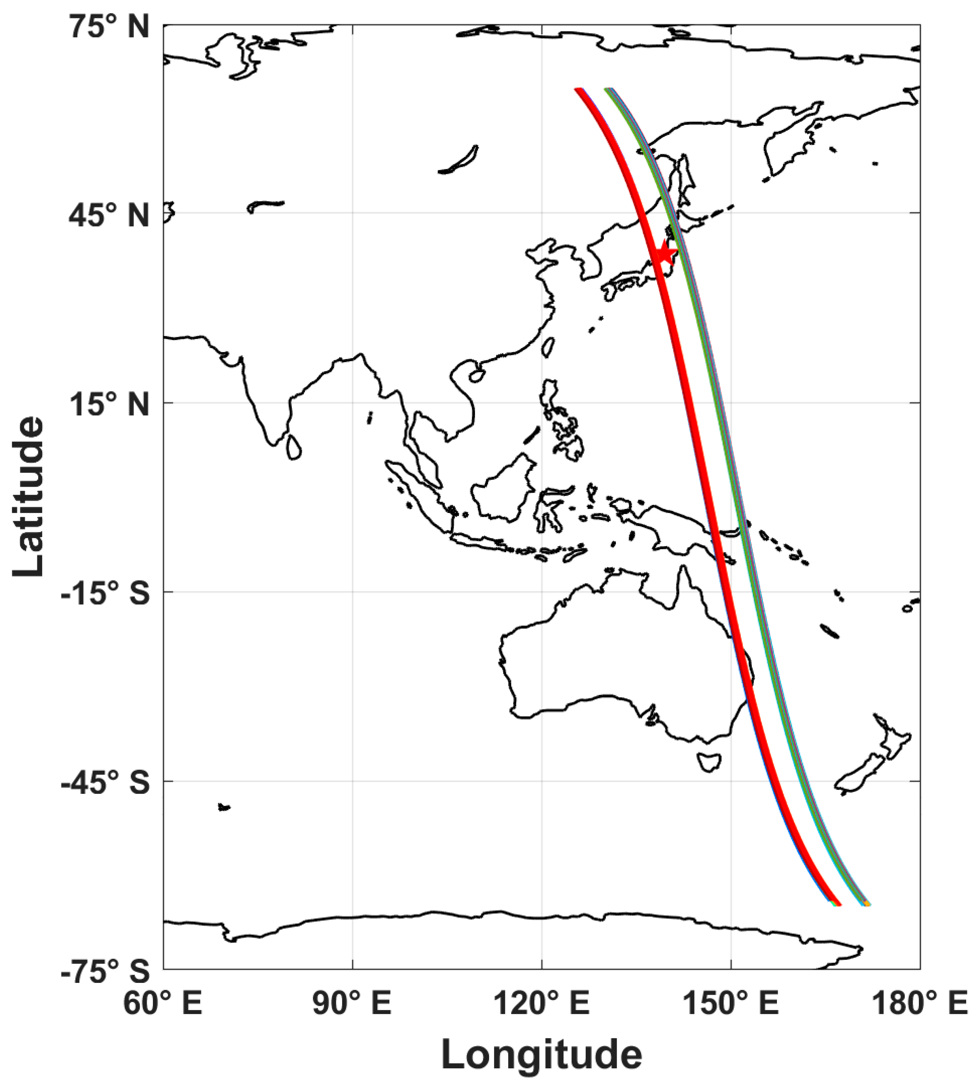
2.1. Selection of the Research Area

In this paper, we selected a region in Northeast Asia within the longitude and latitude ranges of 105° E–145° E and 38° N–58° N, respectively, located at the convergence of the Eurasian, Pacific and North American plates. This region is seismically active and covers China’s only deep seismic zone, encompassing the Northeast Deep Seismic Zone, Tanlu Seismic Zone, Shanxi Seismic Zone, Yanshan Seismic Zone and Hebei Plain Seismic Zone, where several Ms > 5.0 earthquakes have occurred in recent years, including the 1679 Sanhe-Pinggu Ms 8 earthquake, 1976 Tangshan Ms 7.8 earthquake, and 1975 Haicheng Ms 7.5 earthquake, which caused enormous economic losses and casualties [28].

2.2. Selection of Seismic Examples

In this research, we selected Ms > 5.0 earthquakes with depths ≤40 km in the research area from December 2018 to January 2023 (CSES operation time). The seismogenic area of the lithosphere was estimated according to the seismogenic model proposed by Dobrovolsky et al. [29].
ρ = 100.43M
where M is the earthquake magnitude, and ρ is the straight-line distance from the epicenter (the unit is km). The investigated phenomena are Ms > 5.0 earthquakes, so the straight-line distance from the epicenter in the seismogenic area is more than ~142 km (equal to ~1°) according to Equation (1). Seismo-ionospheric perturbation signals can spread from the Earth’s surface to the ionosphere, causing ionosphere perturbations based on the LAIC mechanism. Moreover, seismo-ionospheric perturbation signals may shift in the ionosphere during propagation, and the maximum offset can reach more than 10°. To ensure the credibility of the considered seismic anomalies, we considered that no other Ms > 5.0 earthquakes occurred within the longitude 10° × latitude 10° range around the epicenter from 3 months before to 1 month after the occurrence of the selected earthquakes. A total of 12 typical earthquakes were selected, as listed in Table 1.

2.3. Data Selection

Feng et al. [7] selected second-sampled data of the GM4 fluxgate with a suitable quality, which are 5–100 s cycle data of the 71 geomagnetic observation stations of China’s geomagnetic network. The data were utilized to conduct earthquake predictions with the polarization method, and favorable results were obtained. In this study, we analyzed data recorded by the HPM payload onboard the CSES referring to ground-based data. HPM vector and scalar data are obtained by the Fluxgate Magnetometer (FGM) and Coupled Dark State Magnetometer (CDSM) probes, respectively [30]. In this study, HPM_5 vector data recorded by the FGM probe were selected for seismic analysis. The FGM sampling rate is 1 Hz, the detection band is DC-15 Hz, and the selected data are geomagnetic three-component vector data.

3. Research Methodology

The data recorded by the CSES can be divided into up-orbit data (night side) and down-orbit data (day side), corresponding to approximately 02:00 and 14:00 local time, respectively. To minimize unnecessary perturbations, we selected nighttime data (up-orbit data) for processing and analysis due to the notable influence of solar radiation on the ionosphere during the daytime, which affects the extraction of seismic information [28]. We selected orbital data under the condition of space magnetic disturbance (Dst ≥ −30 nT and Kp < 3). More than 4000 orbits were selected from over 160,000 orbits in this study. The seismogenic area of an Ms > 5.0 earthquake is ~142 km, according to Equation (1). The speed of the CSES is 7.8 km/s, which suggests that it traverses the earthquake area within 18 s. The orbit time of the CSES ranges from 2028 to 2078 s. The perturbation anomaly of the ionosphere generates a certain offset effect, which can produce a shift up to 10°. Therefore, in this paper, the minimum study period was divided into 10 s intervals. That is, every 10 geomagnetic three-component vector data, i.e., the horizontal north–south component, horizontal east-west component, and vertical component, were performed with the Fourier transform to obtain spectral data, respectively, as the FGM sampling rate is 1 Hz. Ground-based data were selected from the second-sampled instrument of GM4 with a period of 5–100 s, i.e., data with a frequency ranging from 0.01 to 0.2 Hz, to extract seismic anomalies [8]. Therefore, in this study, filtering analysis was performed after the above Fourier transform to obtain the dynamic spectrum of the geomagnetic three-component vector data (frequency: 0.01–0.2 Hz) recorded by the HPM probe. The filtering analysis meant that the amplitudes with frequency > 0.2 Hz or <0.01 Hz were all 0. We selected the 0.01–0.2 Hz geomagnetic three-component dynamic spectra recorded by the CSES from 90 days before to 30 days after a given earthquake.
Polarization values N of the observations from 90 days before to 30 days after an earthquake were obtained, along with average polarization values M (with M as the background value) and the mean square S of the polarization values over the 4-year period, according to Equations (2) and (3), respectively. The time series of the perturbation magnitude F of the observations relative to the background values was obtained for analysis according to Equation (4).
H = H x 2 + H y 2
Y z h = Z H
where H x is the north–south spectrum of the geomagnetic horizontal component, H y is the east-west spectrum of the geomagnetic horizontal component, H is the spectrum of the geomagnetic horizontal component, Z is the spectrum of the geomagnetic vertical component, and Y z h is the polarization value (the ratio between vertical component Z and horizontal component H) [7,8,9].
F = (N − M)/S
where N is the polarization value from 90 days to 30 days after a given earthquake, M is the background value, i.e., the average of the polarization values over the 4-year period, and S is the mean square of the polarization values over the 4-year period.

4. Statistical Analysis of Earthquakes

A total of 12 Ms > 5.0 earthquakes were selected within the research area, of which satellite data before and after the Ms 5.4 earthquake off the east coast of Honshu, Japan, on 29 November 2019 were unavailable, so this earthquake was not investigated. The remaining earthquakes were investigated in detail. The 11 earthquakes mentioned above cannot be fully displayed due to the large number of figures. Without loss of representativeness, we describe only the Ms 6.5 earthquake off the west coast of Honshu, Japan, on 18 June 2019, in detail.
An Ms 6.5 earthquake occurred on 18 June 2019, off the west coast of Honshu, Japan, at 38.56° N latitude and 139.52° E longitude at a depth of 20 km. While screening all the up-orbit data for the area around the epicenter, we found two groups of up-orbit trajectories passing near the epicenter, as shown in Figure 1. The pentagram in Figure 1 indicates the epicenter. We found that the western orbital group is closer to the epicenter, while the eastern orbital group is farther away from the epicenter, but both orbital groups occur within 10° of the epicenter. Therefore, these two orbital groups are systematically studied in the following. Notably, the sudden disturbance changes in the results in the region above 50° N and near the region above 50° S were due to the disturbances caused by switching the measurement mode in CSES operation, and these disturbances are retained in this paper.

4.1. Study of the Western Orbital Group Associated with the 18 June 2019, Ms 6.5 Earthquake off the West Coast of Honshu, Japan

Orbit data of the up-orbit group were selected from 90 days before to 30 days after the earthquake under the condition of space magnetic disturbance (Dst ≥ −30 nT and Kp < 3) according to the research method. Then, the spectral time-series data of the three geomagnetic components, i.e., the horizontal north–south component, horizontal east-west component, and vertical component, were filtered, as shown in Figure 2a, Figure 3a and Figure 4a, respectively. The curves with the different colors in the figure represent different periods, i.e., different orbital data, which were limited from −60° S to 60° N from 90 days before to 30 days after the earthquake. The unit is nT/Hz, and the values varied at different latitudes. The spectral time-series data of the three geomagnetic components also have different values at the same latitude at different times in Figure 2a, Figure 3a and Figure 4a, respectively. The Figure 2a and Figure 3a reveal that some perturbation data occurred near the epicenter (the vertical dashed line in the figure indicates the latitude of the earthquake, the red rectangular box indicates the location of the perturbation, and the other subfigures refer to Figure 2a). The north–south and east-west component spectra of the horizontal component within the 10° latitude range from the epicenter from 90 days before to 15 days after the earthquake were subjected to time-series analysis, as shown in Figure 2b and Figure 3b, respectively. In terms of subfigure b, every curve in subfigure b was the amplification from subfigure a within the 10° latitude range from the epicenter from 90 days before to 15 days after the earthquake. The curves with the different colors in subfigure b represent different periods, i.e., different orbital data, which were limited from 28.5° N to 48.5° N. The horizontal dashed line indicates the latitude of the epicenter, the diagonal vertical dashed line indicates the approximate time of the earthquake and the red pentagram indicates the epicenter (refer to Figure 2b for a description of the dashed lines in subfigure b). Notably, the curves had no perturbation prior to 21 May and they were very smooth; however, some anomaly perturbations occurred near 43.5° N after 21 May, as shown in Figure 2b and Figure 3b. The anomaly perturbations gradually moved closer to the epicenter region as the time of the earthquake occurrence approached. Figure 4a shows that there was essentially no seismic disturbance of the vertical component spectral data near the epicenter. Subsequently, we analyzed the time series of the vertical component spectra within the 10° latitude range from the epicenter from 90 days before to 15 days after the earthquake and observed anomaly perturbations near 42° N since 31 May. Moreover, they gradually approached the epicenter as the time of the earthquake occurrence approached, but the intensity was not as high as that of the horizontal component, especially not as high as that of the horizontal east-west component, which agrees with previous studies [24,25,26].
Subsequently, we processed the western orbit data to obtain the time series of the polarization observations (Figure 5) and the time series of the perturbation amplitude (Figure 6) according to Equations (2)–(4), as shown in Figure 5 and Figure 6, respectively. Time-series analysis of the polarization observations revealed anomaly perturbations near the epicenter, before and after the earthquake, which are not as pronounced as those determined via single-component time-series analysis. In addition, time-series analysis of the perturbation amplitude revealed that there were slight perturbations relative to single-component analysis, anomaly perturbations were observed near 42° N from 21 May, and the anomaly perturbation area gradually approached the epicenter as the time of the earthquake occurrence neared.

4.2. Study of the Eastern Orbital Group Associated with the 18 June 2019, Ms 6.5 Earthquake off the West Coast of Honshu, Japan

As shown in Figure 7, Figure 8 and Figure 9, the perturbations along the horizontal north–south and east-west directions in the eastern orbital group data occurred near the epicenter before and after the earthquake. The perturbations along the east-west direction were larger. In contrast, the perturbations were small along the vertical direction, but small perturbations also occurred near the epicenter before and after the earthquake. Anomaly perturbations occurred near 44° N from 22 May, and the anomaly perturbations gradually moved closer to the epicenter as the time of the earthquake occurrence approached, as shown in Figure 7b, Figure 8b and Figure 9b.
As shown in Figure 10 and Figure 11, time-series analysis of the polarization observations revealed that the anomaly perturbations are not as pronounced as the single-component analysis-based perturbations near the epicenter before and after the earthquake. Moreover, anomaly perturbations were observed at approximately 44° N from 22 May. As the time of the earthquake occurrence approached, the anomaly perturbation area moved closer to the epicenter of the earthquake.

4.3. Analysis of Other Earthquakes

Five Ms ≥ 6.0 earthquakes and seven 6.0 > Ms > 5.0 earthquakes were selected in this study, as listed in Table 2 (the negative values represent pre-earthquake date, positive values represent post-earthquake date, the symbol/means no anomaly was observed). Among them, the 29 November 2019, Ms 5.4 earthquake off the east coast of Honshu, Japan, was not investigated due to data quality issues. The anomaly perturbation time of different data for the earthquakes can be summarized as follows (negative values represent pre-earthquake time, positive values represent post-earthquake time):
(1)
In this study, there was no anomaly perturbation when all the data were judged as /. As can be seen from the Table 2, it was recognized that there were no seismic anomaly perturbations before or after the 8 June 2022, Ms5.2 earthquake, the 23 September 2021, Ms5.5 earthquake, both near the Lake Baikal, Russia, or the 12 July 2020, Ms5.1 earthquake in the Guye District, Tangshan, Hebei, China. Therefore, all five Ms ≥ 6.0 earthquakes exhibited anomalies; three of the six 6.0 > Ms > 5.0 earthquakes exhibited anomalies before or after the time of the earthquake occurrence.
(2)
As can be seen in Table 2, the data of horizontal east-west component exhibited anomalies more frequently and the data of the vertical component exhibited anomalies only once in the geomagnetic three-component vector data. Meanwhile, the anomaly perturbation time of the horizontal east-west component was also slightly longer than the others.
(3)
The anomaly perturbations of polarization observations were judged as/more frequently. The anomaly perturbation of polarization perturbation amplitude exhibited anomalies more frequently in Table 2. Among all of the seismic examples with perturbation anomalies, the polarization time-series data exhibited anomalies less frequently, while the polarization perturbation amplitude time series was perturbed more frequently than the polarization time-series data.

5. Discussion

If there is a perturbation source stemming from an earthquake, the vertical component of the geomagnetic field should be drastically perturbed regularly, while most of the horizontal components of the geomagnetic field should be slightly perturbed [6,7,10,31]. In contrast, if there is a perturbation source stemming from the space environment, there should be obvious changes in both the horizontal and vertical components (Figure 12). The geomagnetic pulsations during nighttime are Pi2 and Pc4 and others, which are known to be usually horizontal component [32]. But, if the source of emissions is situated under the ground, we can expect the polarization ratio (the ratio between vertical component Z and horizontal component H) >1, which is found by Kopytenko et al. [33] using the experimental measurements and also by Molchanov and Hayakawa [4] based on theoretical considerations [5]. Therefore, the phenomenon of perturbation changes in the geomagnetic three-component data recorded by the HPM onboard the CSES and ESA Swarm satellites before and after earthquakes, with drastic perturbations of the horizontal component and slight perturbations of the east-west component, must be further described and investigated.
The ionosphere produces an ionospheric equatorial anomaly during the daytime, where the daytime eastward electric field in the E layer (produced by thermal wind drive) can be mapped along magnetic lines to the F layer due to the high parallel conductivity along these magnetic lines. The eastward electric field along the magnetic equator causes plasma to drift upward through E × B. As the plasma rises, it is subjected to gravity and pressure gradient forces that cause it to spread out along the force magnetic lines toward either side of the magnetic equator. The plasma exhibits fountain-like movements under the action of electric field drift and diffusion, referred to as the fountain effect, causing the plasma along the magnetic equator to move toward the geomagnetic latitude of ~±15°, forming a double-peak structure (equatorial ionization anomaly (EIA) crests). The EIA phenomenon disappears at night [34].
LAIC models are roughly categorized into three propagation pathways, including additional DC electric field models and acoustic gravity wave and electromagnetic wave propagation models, each of which induces ionospheric plasma changes in the ionosphere [23]. The CSES flies at an altitude of ~500 km and detects physical parameters related to the F layer of the ionosphere. If the plasma in the D and E layers of the ionosphere near the epicenter, affected by an earthquake, rises to the F layer, it is subjected to gravity and pressure gradient forces, causing the plasma to spread out toward the poles along the force magnetic lines, thereby generating currents along this direction. Then, a change in the horizontal component of the magnetic field is produced, and this physical process could explain the obtained conclusions, i.e., Ampere’s law. The parameters detected by the PAP payload are considerably perturbed before earthquakes [35,36]. To verify the physical mechanism, we studied ion velocity Vx data recorded by the PAP payload onboard the CSES associated with the western orbital group near the epicenter from May to July 2019 (the Vx velocity direction matches the direction of the satellite flight velocity). We selected the up-orbit data, so the satellite flight direction was toward the geographic North Pole. Therefore, the Vx velocity perturbations direction was toward the poles. It was found that the Vx data recorded during the 21 May orbit approximately a month before the earthquake began to exhibit perturbations near the epicenter, which occurred in the same region as the horizontal perturbations of the magnetic field recorded by the HPM, both occurring near 43° N at the same time (Figure 13). The data recorded on June 15 revealed anomalies associated with the Vx data not only within the ±10° range near the epicenter but also in the magnetic conjugate region. In our opinion, that meant the plasma in the D and E layers of the ionosphere near the epicenter rose to the F layer at that moment. Then, a change in the horizontal component of the magnetic field was produced, and the synchronized observation phenomena could explain our conclusions. Moreover, we determined that the Vx data gradually decreased after the earthquake after June 25. In summary, earthquake prediction research can be conducted by combining ion velocity data from the PAP and three-component data of the magnetic field from the HPM in the future. In this research, we also observed that all the Vx perturbations generally occurred as synchronized perturbation phenomena in the magnetic conjugate region, and the underlying physical mechanism should be studied further.

6. Conclusions

We selected 12 typical earthquakes with Ms > 5.0 and epicenter depth ≤ 40 km within the longitude 105° E–145° E and latitude 38° N–58° N range from December 2018 to January 2023 for analysis by using HPM data recorded by the CSES in a quiet magnetic environment. Geomagnetic three-component vector data were selected, and the minimum study period was divided into 10 s intervals. Fourier transform was performed to obtain 0.01–0.2 Hz geomagnetic three-component dynamic spectra, and the time series of the polarization data was then acquired. The average value of the polarization data over four years was used to obtain the time series of the polarization perturbation amplitude, after which we conducted a joint study. The results are as follows:
(1)
All five Ms ≥ 6.0 earthquakes exhibited anomalies, and three of the six 6.0 > Ms > 5.0 earthquakes indicated anomalies before and after the time of earthquake occurrence, indicating that the larger the magnitude, the higher the likelihood that the anomaly perturbation is recorded by the satellite.
(2)
Among all the perturbation anomalies of the investigated earthquakes, the horizontal east-west component indicated the highest perturbation, while the vertical component exhibited the lowest perturbation, which is consistent with the results of previous studies. This suggests that the horizontal east-west component is likely the dominant component of seismic anomaly observations.
(3)
In all the seismic perturbation anomalies, the time series of the polarization data exhibited slight perturbations, suggesting that the polarization method can be better applied to ground-based data but can be applied to space-based data to a lesser degree.
(4)
The polarization perturbation amplitude time series was also slightly perturbed but with a smaller perturbation amplitude than that of the horizontal east-west component. The polarization perturbation amplitude method could be used as a reference method for extracting seismic anomalies.
(5)
Ion velocity Vx data from the plasma analyzer package (PAP) can be considered to approximately verify the physical mechanism of the anomaly perturbation of the horizontal component in the ionospheric magnetic field according to the Ampere’s law, and the two kinds of data (PAP and HPM) can be combined in seismic prediction research.

Author Contributions

Conceptualization, X.O., X.S. and X.Z.; methodology, X.S., M.Y. and X.Z.; software, M.Y. and J.L.; formal analysis, X.Z. and M.Y.; investigation, X.Z. and M.Y.; data curation, T.L., G.Q. and M.Y.; writing—original draft preparation, M.Y.; writing—review and editing, M.Y.; All authors have read and agreed to the published version of the manuscript.

Funding

This research was funded by Earthquake Science and Technology Spark Program (XH23011YA), the Open Fund from Earthquake Forecasting of CEA (XH23080D), Youth Fund Project of Liaoning Earthquake Agency (2022040), Project No. E3RC2TQ5, Project No. E3RC2TQ4, the National Natural Science Foundation of China (42274106), the APSCO Earthquake Research Project Phase II and Earthquake Science and Technology Spark Program (XH23010A).

Institutional Review Board Statement

This study does not require ethical approval.

Informed Consent Statement

Not applicable.

Data Availability Statement

CSES data is available at the website https://www.leos.ac.cn (accessed on 1 March 2023) and the magnetic index are at the website https://omniweb.gsfc.nasa.gov/form/omni_min.html (accessed on 1 March 2023).

Acknowledgments

This paper is supported by Earthquake Science and Technology Spark Program (XH23011YA), the Open Fund from Earthquake Forecasting of CEA (XH23080D), Youth Fund Project of Liaoning Earthquake Agency (2022040), Project No. E3RC2TQ5, Project No. E3RC2TQ4, the National Natural Science Foundation of China (42274106), the APSCO Earthquake Research Project Phase II and Earthquake Science and Technology Spark Program (XH23010A). The authors thank the CSES satellite center (www.leos.ac.cn (accessed on 1 March 2023)) after registration for providing the data. The magnetic index data are from the website of https://omniweb.gsfc.nasa.gov/form/omni_min.html (accessed on 1 March 2023).

Conflicts of Interest

The authors declare no conflict of interest.

References

  1. Moore, G.W. Magnetic disturbances preceding the 1964 Alaska earthquake. Nature 1964, 203, 508–509. [Google Scholar] [CrossRef]
  2. Ouyang, X.Y.; Parrot, M.; Bortnik, J. ULF wave activity observed in the nighttime ionosphere above and some hours before strong earthquakes. J. Geophys. Res. Space Phys. 2020, 125, e2020JA028396. [Google Scholar] [CrossRef]
  3. Yumoto, K.; Ikemoto, S.; Cardinal, M.G.; Hayakawa, M.; Hattori, K.; Liu, J.Y.; Saroso, S.; Ruhimat, M.; Husnig, M.; Widarto, D.; et al. A new ULF wave analysis for seismo-electromagnetics using CPMN/MAGDAS data. Phys. Chem. Earth Parts A/B/C 2009, 34, 360–366. [Google Scholar] [CrossRef]
  4. Molchanov, O.A.; Hayakawa, M. Generation of ULF electromagnetic emissions by microfracturing. Geophys. Res. Lett. 1995, 22, 3091–3094. [Google Scholar] [CrossRef]
  5. Hayakawa, M.; Kawate, R.; Molchanov, O.A.; Yumoto, K. Results of ultra-low-frequency magnetic field measurements during the Guam earthquake of 8 August 1993. Geophys. Res. Lett. 1996, 23, 241–244. [Google Scholar] [CrossRef]
  6. Hattori, K. ULF geomagnetic changes associated with large earthquakes. Terr. Atmos. Oceanic. Sci. 2004, 15, 329–360. [Google Scholar] [CrossRef]
  7. Feng, Z.S.; Li, Q.; Lu, J.; Li, H.; Ju, H.; Sun, H.; Yang, F.; Zhang, Y. The Seismic ULF Geomagnetic Reliable Information Exaction Based on Fluxgate Magnetometer Data of Second Value. South China J. Seismol. 2010, 30, 1–7. [Google Scholar]
  8. He, C.; Feng, Z.S. Application of polarization method to geomagnetic data from the station Chengdu. Acta Seismol. Sin. 2017, 39, 558–564. [Google Scholar] [CrossRef]
  9. Fan, W.J.; Feng, L.L.; Li, X.; He, C.; Liao, X.F.; Yao, X.Y. Characteristics of geomagnetic vertical intensity polarization anomalies before Menyuan, Qinghai Ms6.9 earthquake on 8 January 2022. J. Earthq. Eng. J. 2022, 44, 744–75010. [Google Scholar]
  10. Han, P.; Katsumi, H.; Maiko, H.; Jiancang, Z.; Chieh-Hung, C.; Febty, F.; Hiroki, Y.; Chie, Y.; Jann-Yenq, L.; Shuji, Y. Statistical analysis of ULF seismomagnetic phenomena at Kakioka, Japan, during 2001–2010. J. Geophys. Res. Space Phys. 2014, 119, 4998–5011. [Google Scholar] [CrossRef]
  11. Varotsos, P.V.; Sarlis, N.V.; Skordas, E.S. Electric Fields that “arrive” before the time derivative of the magnetic field prior to major earthquakes. Phys. Rev. Lett. 2003, 91, 148501. [Google Scholar] [CrossRef] [PubMed]
  12. Sarlis, N.V. Statistical Significance of Earth’s Electric and Magnetic Field Variations Preceding Earthquakes in Greece and Japan Revisited. Entropy 2018, 20, 561. [Google Scholar] [CrossRef]
  13. Feng, Y.; An, Z.; Sun, H.; Mao, F. Geomagnetic survey satellites. Prog. Geophys. 2010, 25, 1947–1958. (In Chinese) [Google Scholar]
  14. Shen, X.; Zhang, X.; Cui, J.; Zhou, X.; Jiang, W.; Gong, L.; Li, Y.; Liu, Q. Remote sensing application in earthquake science research and geophysical fields exploration satellite mission in China. J. Remote Sens. 2018, 22, 1–16. [Google Scholar]
  15. Dolginov, S.; Zhuzgov, L.N.; Pushkov, N.V.; Tyurmina, L.O.; Fryazinov, I.V. Some results of measurements of the constant geomagnetic field above the USSR from the third artificial Earth satellite. Geomagn. Aeron. 1962, 2, 877–889. [Google Scholar]
  16. Langel, R.; Ousley, G.; Berbert, J.; Murphy, J.; Settle, M. The MAGSAT mission. Geophys. Res. Lett. 1982, 9, 243–245. [Google Scholar] [CrossRef]
  17. Neubert, T.; Mandea, M.; Hulot, G.; Von Frese, R.; Primdahl, F.; Jørgensen, J.L.; Friis-Christensen, E.; Stauning, P.; Olsen, N.; Risbo, T. Ørsted satellite captures high-precision geomagnetic field data. Eos Trans. Am. Geophys. Union 2001, 82, 81–88. [Google Scholar] [CrossRef]
  18. Reigber, C.; Lühr, H.; Schwintzer, P. CHAMP mission status. Adv. Space Res. 2002, 30, 129–134. [Google Scholar] [CrossRef]
  19. Friis-Christensen, E.; Lühr, H.; Hulot, G. Swarm: A constellation to study the Earth’s magnetic field. Earth Planets Space 2006, 58, 351–358. [Google Scholar] [CrossRef]
  20. Parrot, M.; Benoist, D.; Berthelier, J.; Błęcki, J.; Chapuis, Y.; Colin, F.; Elie, F.; Fergeau, P.; Lagoutte, D.; Lefeuvre, F.; et al. The magnetic field experiment IMSC and its data processing onboard DEMETER: Scientific objectives, description and first results. Planet. Space Sci. 2006, 54, 441–455. [Google Scholar] [CrossRef]
  21. Liu, J.; Guan, Y.B.; Zhang, X.M.; Shen, X.H. The data comparison of electron density between CSES and DEMETER satellite, swarm constellation and IRI model. Earth Space Sci. 2021, 8, e2020EA001475. [Google Scholar] [CrossRef]
  22. Shen, X.; Huang, J.; Lin, J.; Luo, Z.; Le, H.; Wu, L.; Zhang, X.; Cui, J. Project plan and research on data analysis and processing technology of geophysical exploration satellite and application research of earthquake prediction. Prog. Earthq. Sci. 2022, 52, 1–25. [Google Scholar] [CrossRef]
  23. Zhang, X.M.; Shen, X.H. The development in seismo-ionospheric coupling mechanism. Prog. Earthq. Sci. 2022, 52, 193–202. [Google Scholar] [CrossRef]
  24. De Santis, A.; Balasis, G.; Pavón-Carrasco, F.J.; Cianchini, G.; Mandea, M. Potential earthquake precursory pattern from space: The 2015 Nepal event as seen by magnetic Swarm satellites. Earth Planet. Sci. Lett. 2017, 461, 119–126. [Google Scholar] [CrossRef]
  25. Marchetti, D.; De Santis, A.; D’Arcangelo, S.; Poggio, F.; Jin, S.; Piscini, A. Magnetic field and electron density anomalies from swarm satellites preceding the major earthquakes of the 2016–2017 Amatrice-Norcia (Central Italy) seismic sequence. Pure Appl. Geophys. 2019, 177, 305–319. [Google Scholar] [CrossRef]
  26. Pinheiro, K.J.; Jackson, A.; Finlay, C.C. Measurements and uncertainties of the occurrence time of the 1969, 1978, 1991, and 1999 geomagnetic jerks. Geochem. Geophys. Geosyst. 2011, 12, Q10015. [Google Scholar] [CrossRef]
  27. Ouyang, X.-Y.; Wang, Y.-F.; Zhang, X.-M.; Wang, Y.-L.; Wu, Y.-Y. A New Analysis Method for Magnetic Disturbances Possibly Related to Earthquakes Observed by Satellites. Remote Sens. 2022, 14, 2709. [Google Scholar] [CrossRef]
  28. Yang, M.; Qian, G.; Zhang, X.; Shen, X.; Zhang, M.; Jin, Y. Study on abnormal electromagnetic wave associated with Magnitude Ms≥6.0 in Northeast Asia. J. Geod. Geodyn. 2022, 42, 669–674. [Google Scholar] [CrossRef]
  29. Dobrovolsky, I.P.; Zubkov, S.I.; Miachkin, V.I. Estimation of the size of earthquake preparation zones. Pure Appl. Geophys. 1979, 117, 1025–1044. [Google Scholar] [CrossRef]
  30. Yang, Y.; Zhou, B.; Hulot, G.; Olsen, N.; Wu, Y.; Xiong, C.; Stolle, C.; Zhima, Z.; Huang, J.; Zhu, X.; et al. CSES high precision magnetometer data products and example study of an intense geomagnetic storm. J. Geophys. Res. Space Phys. 2021, 126, e2020JA028026. [Google Scholar] [CrossRef]
  31. Sarlis, N.; Varotsos, P. Magnetic field near the outcrop of an almost horizontal conductive sheet. J. Geodyn. 2002, 33, 463–476. [Google Scholar] [CrossRef]
  32. Saito, T. Geomagnetic Pulsations. Space Sci. Rev. 1969, 10, 319–412. [Google Scholar] [CrossRef]
  33. Kopytenko, Y.A.; Matiashvili, T.G.; Voronov, P.M.; Kopytenko, E.A. Observation of electromagnetic ultralow frequency lithospheric emissions in the Caucasian seismically active zone and their connection with earthquakes. In Electromagnetic Phenomena Related to Earthquake Prediction; Hayakawa, M., Fujinawa, Y., Eds.; Narosa Publishing House: New Delhi, India, 1994; pp. 175–180. [Google Scholar]
  34. Xiong, N.L.; Tang, C.S.; Li, X.J. Introduction to Ionospheric Physics; Wuhan University Press: Wuhan, China, 1999; Volume 6–14, pp. 53–57. [Google Scholar]
  35. Liu, D.; Zeren, Z.; Shen, X.; Zhao, S.; Yan, R.; Wang, X.; Liu, C.; Guan, Y.; Zhu, X.; Miao, Y.; et al. Typical ionospheric disturbances revealed by the plasma analyzer package onboard the China Seismo-Electromagnetic Satellite. Adv. Space Res. 2021, 68, 3796–3805. [Google Scholar] [CrossRef]
  36. Li, M.; Shen, X.; Parrot, M.; Zhang, X.; Zhang, Y.; Yu, C.; Yan, R.; Liu, D.; Lu, H.; Guo, F.; et al. Primary joint statistical seismic influence on ionospheric parameters recorded by the CSES and DEMETER satellites. J. Geophys. Res. Space Phys. 2020, 125, e2020JA028116. [Google Scholar] [CrossRef]
Figure 1. Two groups of CSES up-orbit trajectories near the 18 June 2019, Ms 6.5 earthquake off the west coast of Honshu, Japan.
Atmosphere 14 01555 g001
Figure 2. Horizontal north-south component spectral time series of the western orbital group associated with the 18 June 2019, Ms 6.5 earthquake off the west coast of Honshu, Japan. (a) Horizontal north–south component spectral time series from 90 days before to 30 days after the earthquake. (b) Horizontal north–south component spectral time series from 90 days before to 15 days after the earthquake within the 10° latitude range from the epicenter.
Atmosphere 14 01555 g002
Figure 3. Horizontal east-west component spectral time series of the western orbital group associated with the 18 June 2019, Ms 6.5 earthquake off the west coast of Honshu, Japan. (a) Horizontal east-west component spectral time series from 90 days before to 30 days after the earthquake. (b) Horizontal east-west component spectral time series from 90 days before to 15 days after the earthquake within the 10° latitude interval from the epicenter.
Atmosphere 14 01555 g003
Figure 4. Vertical component spectral time series of the western orbital group associated with the 18 June 2019, Ms 6.5 earthquake off the west coast of Honshu, Japan. (a) Vertical component spectral time series from 90 days before to 30 days after the earthquake. (b) Vertical component spectral time series from 90 days before to 15 days after the earthquake within the 10° latitude range from the epicenter.
Atmosphere 14 01555 g004
Figure 5. Polarization spectral time series of the western orbital group associated with the 18 June 2019, Ms 6.5 earthquake off the west coast of Honshu, Japan. (a) Polarization spectral time series from 90 days before to 30 days after the earthquake. (b) Polarization spectral time series from 90 days before to 15 days after the earthquake within the 10° latitude range from the epicenter.
Atmosphere 14 01555 g005
Figure 6. Spectral time series of the polarization perturbation amplitude of the western orbital group associated with the 18 June 2019, Ms 6.5 earthquake off the west coast of Honshu, Japan. (a) Scheme 90. days before to 30 days after the earthquake. (b) Scheme 90. days before to 15 days after the earthquake within the 10° latitude range from the epicenter.
Atmosphere 14 01555 g006
Figure 7. Horizontal north–south component spectral time series of the eastern orbital group associated with the 18 June 2019, Ms 6.5 earthquake off the west coast of Honshu, Japan. (a) Horizontal north–south component spectral time series from 90 days before to 30 days after the earthquake. (b) Horizontal north–south component spectral time series from 90 days before to 15 days after the earthquake within the 10° latitude range from the epicenter.
Atmosphere 14 01555 g007
Figure 8. Horizontal east-west component spectral time series of the eastern orbital group associated with the 18 June 2019, Ms 6.5 earthquake off the west coast of Honshu, Japan. (a) Horizontal east-west component spectral time series from 90 days before to 30 days after the earthquake. (b) Horizontal east-west component spectral time series from 90 days before to 15 days after the earthquake within the 10° latitude range from the epicenter.
Atmosphere 14 01555 g008
Figure 9. Vertical component spectral time series of the eastern orbital group associated with the 18 June 2019, Ms 6.5 earthquake off the west coast of Honshu, Japan. (a) Vertical component spectral time series from 90 days before to 30 days after the earthquake. (b) Vertical component spectral time series from 90 days before to 15 days after the earthquake within the 10° latitude range from the epicenter.
Atmosphere 14 01555 g009
Figure 10. Polarization spectral time series of the eastern orbital group associated with the 18 June 2019, Ms 6.5 earthquake off the west coast of Honshu, Japan. (a) Polarization spectral time series from 90 days before to 30 days after the earthquake. (b) Polarization spectral time series from 90 days before to 15 days after the earthquake within the 10° latitude range from the epicenter.
Atmosphere 14 01555 g010
Figure 11. Spectral time series of the polarization perturbation amplitude of the eastern orbital group associated with the 18 June 2019, Ms 6.5 earthquake off the west coast of Honshu, Japan. (a) Scheme 90. days before to 30 days after the earthquake. (b) Scheme 90. days before to 15 days after the earthquake within the 10° latitude range from the epicenter.
Atmosphere 14 01555 g011
Figure 12. Geomagnetic polarization mechanism model.
Atmosphere 14 01555 g012
Figure 13. Time series variation in the ion velocity along the CSES flight direction with western orbiting data from 21 May to 30 July 2019.
Atmosphere 14 01555 g013
Table 1. Catalog of the selected Ms > 5.0 earthquakes in Northeast Asia, December 2018–January 2023.
Magnitude (Ms)UTC+8Longitude (°)Latitude (°)Depth (km)Location
15.114 October 2022
08:53:53
105.7552.0510Lake Baikal region, Russia
25.28 June 2022
20:24:18
105.7552.1010Lake Baikal region, Russia
35.323 May 2022
10:01:03
143.1541.1010Off the east coast of Honshu, Japan
45.523 September 2021
01:01:26
117.8056.3510East of Lake Baikal, Russia
56.61 May 2021
09:27:26
141.9038.2530Off the east coast of Honshu, Japan
66.321 December 2020
01:23:19
142.7540.7510Off the east coast of Honshu, Japan
75.112 July 2020
06:38:25
118.4439.7810Guye District, Tangshan, Hebei, China
86.220 April 2020
04:39:05
142.1038.9130Off the east coast of Honshu, Japan
95.429 November 2019
12:01:36
143.1139.1910Far from the east coast of Honshu, Japan
106.518 June 2019
21:22:21
139.5238.5620Off the west coast of Honshu, Japan
115.118 May 2019
06:24:48
124.7545.3010Ningjiang District, Songyuan city, Jilin
126.011 April 2019
16:18:23
143.4040.3510Far from the east coast of Honshu, Japan
Table 2. Polarization method-based research on magnetic field data associated with other 12 earthquakes in Northeast Asia.
UTC+8LocationMagnitude (Ms)The Anomaly Perturbation Time of Horizontal North–South Component
(Hx)
The anomaly Perturbation Time of Horizontal East–West Component
(Hy)
The Anomaly Perturbation Time of the Vertical Component
(Z)
The Anomaly Perturbation Time of Polarization Observation
(N)
The Anomaly Perturbation Time of Polarization Perturbation Amplitude
(F)
114 October 2022
08:53:53
Lake Baikal region, Russia5.1/−8 days///
28 June 2022
20:24:18
Lake Baikal region, Russia5.2/////
323 May 2022
10:01:03
Off the east coast of Honshu, Japan5.3/−17 days to 23 days/−2 days to 17 days−17 days to 23 days
423 September 2021
01:01:26
East of Lake Baikal, Russia5.5/////
51 May 2021
09:27:26
Off the east coast of Honshu, Japan6.615 days to 30 days15 days to 30 days//20 days to 30 days
621 December 2020
01:23:19
Off the east coast of Honshu, Japan6.3/1 days to 20 days//1 days
712 July 2020
06:38:25
Guye District, Tangshan, Hebei, China5.1/////
820 April 2020
04:39:05
Off the east coast of Honshu, Japan6.26 days to 26 days6 days to 26 days///
929 November 2019
12:01:36
Far from the east coast of Honshu, Japan5.4/////
1018 June 2019
21:22:21
Off the west coast of Honshu, Japan6.5−28 days to 12 days−28 days to 12 days−21 days to 12 days−28 days to 12 days−28 days to 12 days
1118 May 2019
06:24:48
Ningjiang District, Songyuan city, Jilin5.1−14 days to 30 days−19 days to 30 days///
1211 April 2019
16:18:23
Far from the east coast of Honshu, Japan6.0/−29 days/−29 days/
Disclaimer/Publisher’s Note: The statements, opinions and data contained in all publications are solely those of the individual author(s) and contributor(s) and not of MDPI and/or the editor(s). MDPI and/or the editor(s) disclaim responsibility for any injury to people or property resulting from any ideas, methods, instructions or products referred to in the content.

