Assessing the Accuracy of 3D-VAR in Supercell Thunderstorm Forecasting: A Regional Background Error Covariance Study

Abstract

Data assimilation (DA) integrates observational data with numerical weather predictions to enhance weather forecast accuracy. This study evaluates three regional background error (BE) covariance statistics for numerical weather prediction (NWP) via a variational data assimilation (VAR) scheme. The best practices in DA are highlighted, as well as the impact of BE covariance calculation in DA procedures by employing the Weather Research and Forecasting (WRF) model. Forecasts initialized at different intervals were used to compute distinct regional background error statistics utilizing three control variable (CV) methodologies over a span of 20 days. These statistics are used by the three-dimensional VAR DA process of WRF DA software, producing analysis fields that lead to forecasts for a distinct convective supercell event during the summer of 2019 over northern Greece. This high-impact convective event underscores the importance of selecting appropriate BE over complex terrain areas. The results emphasize the significance of BE usage in DA, proposing the optimal DA approach for simulations of convective systems.

1. Introduction

Several methods are widely used for the objective of state estimation based on the weighted combination of different sources of information. The process of data assimilation (DA) refines forecasts by incorporating atmospheric observations and estimated errors in both observations and forecasts [1,2]. This leads to an optimal estimate of the initial state for numerical weather prediction (NWP) models, achieved through the combination of available information sources, including prior model forecasts and observations while considering uncertainties [3]. To enhance the accuracy of forecasts, DA methodologies can play a pivotal role by combining the limited observations with the model’s first guess while accommodating uncertainties inherent in each information source.

The three-dimensional variational data assimilation (3D-VAR) DA systems include the Gridpoint Statistical Interpolation (GSI) developed by the National Centers for Environmental Prediction (NCEP), the Variational Analysis System by the European Centre for Medium-Range Weather Forecasts (ECMWF), and the Local Ensemble Transform Kalman Filter (LETKF) by the University of Maryland. In this spectrum, the WRF VAR system has a significant influence due to its versatile control variable (CV) options.

Optimal blending of observations with atmospheric model data results in an improved model initial state. This is particularly significant considering the relatively small amount of observations compared to the degrees of freedom of a forecast model’s initial state [4]. The incorporation of surface observations into NWP models has demonstrated the potential to improve the model’s performance. Previous studies have aimed to refine simulations of weather parameters by assimilating both direct and modeled surface observations, including temperature, water vapor, mixing ratio, and wind [5]. Additionally, assimilating data such as 2 m potential temperature, 2 m dew point temperature, and 10 m wind observations have been explored for determining planetary boundary layer (PBL) profiles [6]. European Center for Medium-Range Weather Forecasts (ECMWF) pioneered the direct assimilation of high-resolution satellite data, including microwave radiance affected by precipitation [7,8,9,10]. Furthermore, studies have shown the possible improvement in rainfall forecasts from NWP models by assimilating radar reflectivity [11,12,13] or radar-derived precipitation data [14,15]. However, it is crucial to validate remote sensing data against ground truth [16]. Surface observations offer a valuable resource for simulating mesoscale weather phenomena [17]. Notably, observations alone are inadequate for estimating background errors (BE) due to their scattered grid.

The effectiveness of the 3D-VAR DA systems relies on their operational mechanisms; part of them is the role of BE within variational schemes. In VAR schemes, BE provides information to balance the influence of the observations on the model forecasts in space and intensity. The accuracy of the DA solution depends highly on the representation of the observation error, which describes uncertainties in the numerical model forecasts prior to new observation incorporation.

Estimation of BE varies depending on the chosen methodology [18]. One prevalent approach involves deriving BE covariances from innovation vectors, which are disparities between observed values and corresponding background state equivalents [19]. This method operates with the assumption of known spatial structures of observation errors and considers dynamic balance assumptions between variables. Another common practice is using statistics of forecast differences as approximations for forecast error covariances, often referred to as the “NMC method” [20]. Alternatively, the use of time-averaged covariances of an extended Kalman filter has been explored, although this demands more computational resources [21]. Variants of Kalman filter-based techniques, such as the reduced rank Kalman filter and ensemble Kalman filter, offer means to attain synoptically dependent background error characteristics [22]. Additionally, the maximum likelihood theory employs a covariance model fit to innovation vectors [23]. Notably, the WRF model is frequently employed to calculate BE and perform DA experiments using model forecasts initialized at different times. Accurate estimation of BE is essential for the success of DA, as it ensures appropriate weighting to background information, implicitly considering observations [24]. Additionally, BEs are spatially correlated, enabling the propagation of observational information in three dimensions. Moreover, these BEs for various meteorological variables demonstrate correlation, allowing multivariate adjustments that reflect atmospheric balance [25,26].

The utility of the WRF model is connected with the accuracy of initial and boundary conditions. The BEs are tied to the choice of control variables, which inherently influence the assimilation and, consequently, the prediction processes. For this reason, the latest version of the WRF model and WRF VAR is employed in the present study. As part of our methodological analysis, we employ detailed meteorological observations, only surface observations at this stage as a first attempt, which are processed, assimilated, and tested under various configurations, primarily focusing on three different control variable (CV) options under WRF DA, introducing differences in thermodynamic correlations of BE estimation. By comparing the outcomes from multiple 3D-VAR DA runs, the relative advantages and limitations of each CV choice are indicated, particularly at the near-surface layers, where the forecast differences are more evident due to the use of only surface observations. These CV options provide frameworks for atmospheric model state variable analysis, and their choice can influence the accuracy of model predictions at various spatial scales. The diverse nature of these CV options underlines the flexibility of the WRF VAR system, catering to various meteorological scenarios and scales. While each option has its strengths, their selection based on specific requirements can play a critical role in optimizing weather forecasts.

In an attempt to examine the aspect of different BE outcomes, a high-impact convective case, with characteristics of a supercell system, was selected that affected northern Greece. As far as the predictability of such phenomena, global models struggled to forecast this event accurately. On the other hand, mesoscale models, which are crucial for NWP, rely on global models for initial conditions. Analyzing control variable (CV) options’ impact on model predictions, especially in complex meteorological scenarios such as the present study, allows us to assess their accuracy and efficacy, particularly for extreme events like supercells.

With the increasing frequency and intensity of extreme weather events [27,28,29,30,31], it is necessary to refine our meteorological models for more precise forecasts. The main goal is not just to understand the behavior of this specific event but also to distill insights that could enhance the operational reliability of the application of the WRF system in future events. The goal of this investigation is dual: firstly, to discern these variations, and secondly, to strive for the optimization of initial conditions in NWP results. This study aims mainly at exploring the effects of CVs in producing and assessing the different scales of the meteorological phenomena present in such a complex case study and hence providing the best initial conditions using at first only surface observations rather than reproducing or modeling the exact weather event in a model environment. It specifically highlights the best practice regarding the usage of CVs in extreme weather events where convective phenomena are present, especially considering areas with complex terrain, such as Greece. As a further outcome, it is to provide suggestions for introducing a best practice for future data assimilation of multi-site and multi-level observations, such as radar data, in order to reproduce the event having a more complete observational dataset.

The paper is structured as follows: Section 2 provides an overview of BE and 3D-VAR data assimilation background necessary for the purposes of this paper. In Section 3, the meteorological test case is presented. Section 4 presents a concise description of the methodology and experiment design. The results of the DA experiments are analyzed and evaluated in Section 5, and the findings are summarized in the concluding Section 6.

2. Data Assimilation and Background Error Theory

The 3D-VARDA approach is a technique used in NWP to improve the accuracy of weather forecasts. It uses a mathematical optimization scheme called variational data assimilation (VAR). The technique uses observational data to interact with numerical weather model forecasts, producing a best estimate and, hence, a more accurate analysis of the initial weather conditions as initial conditions to NWP. VAR schemes play an important role in the initialization of NWP forecasts by providing high-resolution information on the horizontal and vertical components of the atmosphere, especially in areas where there is no adequate observation coverage or in areas that suffer from terrain complexity.

2.1. The 3D-VARDA Approach

The WRF-3D-VAR system developed by Barker et al. [32] is used in this study in tandem with the WRF model for assimilating surface observations. In mathematical terms, the 3D-VAR method can be represented as a minimization problem, where the objective function is the sum of the squared differences between the observations and the model’s background state plus a regularization term that accounts for the background errors. The cost function J is defined as the sum of the background error variance and the observation error variance. The minimization is performed over the atmospheric state, called state vector x. The performance of the DA system largely depends on the plausibility of the BE covariance. The $\mathrm{J}$ cost function can be defined as:

$$\mathrm{J}\left(\mathrm{x}\right)={\mathrm{J}}_{\mathrm{b}}+{\mathrm{J}}_0=\frac{1}{2}{\left(\mathrm{x}-{\mathrm{x}}^{\mathrm{b}}\right)}^{\mathrm{T}}{\mathrm{B}}^{-1}\left(\mathrm{x}-{\mathrm{x}}^{\mathrm{b}}\right)+\frac{1}{2}{\left(\mathrm{y}-\mathrm{H}\left(\mathrm{x}\right)\right)}^{\mathrm{T}}{\mathrm{R}}^{-1}\left(\mathrm{y}-\mathrm{H}\left(\mathrm{x}\right)\right)$$

(1)

where ${\mathrm{x}}^{\mathrm{b}}$ is the background state vector, $\mathrm{B}$ is the BE covariance matrix, $\mathrm{y}$ is the observation vector, $\mathrm{H}$ is the observation operator, and $\mathrm{R}$ is the observation error covariance matrix [33].

The direct calculation of the background term ${\mathrm{J}}_{\mathrm{b}}$ for a numerical weather model with typically 10⁷ degrees of freedom is not possible because the requirement increases the computational cost significantly. To reduce the computational cost, ${\mathrm{J}}_{\mathrm{b}}$ is calculated in terms of control variable vectors, defined via the relation $\mathrm{x}{}^{\prime }=\mathrm{U}\mathrm{v}$, where $\mathrm{x}{}^{\prime }$ denotes the analysis increment, ${\mathrm{x}}^{\prime }=\mathrm{x}-{\mathrm{x}}^{\mathrm{b}}$. Using the incremental formulation [32,34] and the control variable transform, Equation (1) can be rewritten as:

$$\mathrm{J}={\mathrm{J}}_{\mathrm{b}}+{\mathrm{J}}_0=\frac{1}{2}{\mathrm{v}}^T\mathrm{v}+\frac{1}{2}{\left(\mathrm{y}{}^{\prime }-\mathrm{H}\mathrm{U}\mathrm{v}\right)}^{\mathrm{T}}{\mathrm{R}}^{-1}\left(\mathrm{y}{}^{\prime }-\mathrm{H}\mathrm{U}\mathrm{v}\right)$$

(2)

where ${\mathrm{y}}^{\prime }=\mathrm{y}-\mathrm{H}\left(\mathrm{x}\right)$ is the innovation vector [33]. The transformation matrix $\mathrm{U}$ is defined in such a way that the BE matrix can be represented as ${\mathrm{U}\mathrm{U}}^{\mathrm{T}}$. In the WRF 3D-VAR system, the control variable vector is implemented in three steps: a horizontal transform, $U_{\mathrm{h}}$, a vertical transform, $U_{\mathrm{v}},$ and a parameter transform, $U_{\mathrm{p}}$: ${\mathrm{x}}^{\prime }=\mathrm{U}\mathrm{v}=U_{\mathrm{h}}{U}_{\mathrm{v}}{U}_{\mathrm{p}}\mathrm{v}$[32].

2.2. Background Error Disciplines

Using control variables for background error covariances, it is necessary to generate specific, domain-dependent BE. The input data needed for the calculation of BE are WRF forecasts, which are used to generate model perturbations and were used as a proxy for estimates of forecast error. For the NMC method, the model perturbations are differences between forecasts (e.g., T + 24 minus T + 12 is typical for regional applications) valid at the same time. Climatological estimates of BE may then be obtained by averaging these forecast differences over a period of time (e.g., one month).

The background error covariances estimated are not directly used in a VAR DA system. In the WRF VAR system, a control variable transform $\mathrm{x}{}^{\prime }=\mathrm{U}\mathrm{v}$ is used to model background errors, where $\mathrm{v}$ represents the control variable vector and $\mathrm{x}{}^{\prime }$ stands for the analysis increment vector. Finally, $\mathrm{U}$ is used to map the transform of control variables from control space to analysis space. The control variable $\mathrm{x}{}^{\prime }=\mathrm{U}\mathrm{v}$ is implemented through a series of operations ${\mathrm{x}}^{\prime }=U_{\mathrm{h}}{U}_{\mathrm{v}}{U}_{\mathrm{p}}\mathrm{v}$ [32]. The control variables aim to convert the BE covariance matrix into blockdiagonal form. The WRF VAR system provides the balance relations between the new set of variables using regression relations. After the “balanced part” of analysis variables is estimated, the “unbalanced part” is determined by subtracting the former from the full fields. Hence, while some fields are analyzed in full, for some other variables, the unbalanced parts are included in the analysis system.

The horizontal transform $U_{\mathrm{h}}$ is to model the auto-correlation of control variables using recursive filters [35,36] in WRF 3D-VAR. The horizontal correlations are assumed to be homogeneous (i.e., not dependent on geographic position) and isotropic for each control variable. There are two free parameters associated with each variable for the recursive filter: the number of applications and its correlation length. The correlation length scale is estimated for each variable and vertical mode using the NMC method’s accumulated forecast difference data processed as a function of gridpoint separation [32]. A tuning factor is applied to the length scale in order to reflect the actual correlation length scales in a domain.

The vertical transform $U_{\mathrm{v}}$ is performed via an empirical orthogonal function (EOF) decomposition of the vertical component of background error on model levels. The analysis increments are projected onto the eigenvector space, and the eigenvalues specify the relative weights of increments in the calculation of the cost function.

The physical variable transform $U_{\mathrm{p}}$ involves balance transform and conversion of control variables to analysis variable increments. The parameter transformation $U_{\mathrm{p}}$ is applied so that the errors in the control variables are not correlated with each other.

Commonly used options are CV3, CV5, CV6, and CV7, available in WRF DA. A default CV3 BE file is provided with the WRF DA source code as a generic option with no domain dependence. Domain-dependent options CV5, CV6, and CV7 utilize different control variables. CV5 option utilizes streamfunction (ψ), unbalanced velocity potential (χ_u), unbalanced temperature (t_u), pseudo-relative humidity (rh_s), and unbalanced surface pressure (ps_u). CV6 option is similar to CV5, but it has six extra correlation coefficients in the definition of the balanced part of analysis control variables, as well as the moisture control variables is the unbalanced portion of the pseudo-relative humidity (rh_s,u). CV7 option uses a different set of control variables, which are u, v, temperature, pseudo-relative humidity (rh_s), and surface pressure (ps).

Table 1. Control variable configurations across different options.

CV Option	Control Variables
CV3	ψ, χu, tu, q, psu
CV5	ψ, χu, tu, rhs, psu
CV6	ψ, χu, tu, rhs,u, psu
CV7	u, v, t, rhs, ps

outlines the specific atmospheric CV associated with each configuration option.

The BE estimation for a specific domain consists of five stages generated via the NMC method [20]. The first step is the calculation of standard perturbations from forecast differences as x’ = xT2 − xT1, where xT2 and xT1 are forecast difference times (24 and 12 h for this regional case study). The second step is to remove the time and bin mean values for each variable and level, ending with zero-mean fields. The third step is a regression analysis between the control variables, depending on the configuration between CV5, CV6, and CV7, returning the unbalanced components of each field calculated. The fourth step is to calculate the vertical component of the control variables, and finally, the fifth step is the calculation of horizontal correlations for the control variables using recursive filters.

The option CV5 [32] uses the stream function and unbalanced velocity potential as primary control variables. Its approach primarily revolves around independent variables, ensuring that each component (e.g., temperature, surface pressure) is treated separately without substantial inter-variable influences. In this option, the analysis variables consist of the full fields corresponding to stream function and relative humidity and the unbalanced parts corresponding to the other variables included in the analysis. In the CV5 option, temperature and surface pressure are not related to each other nor to the moisture variable. The relative humidity field is not influenced by any of the model variables like temperature or wind. The statistical balance transform is defined by:

$$\left(\begin{array}{c}\psi \\ \chi \\ \begin{array}{c}t\\ \begin{array}{c}ps\\ rh\end{array}\end{array}\end{array}\right)=\left(\begin{array}{c}\mathrm{I}\\ {\mathrm{C}}_{\mathsf{\chi },\mathsf{\psi }}\\ \begin{array}{c}{\mathrm{C}}_{\mathrm{t},\mathsf{\psi }}\\ \begin{array}{c}{\mathrm{C}}_{\mathrm{p}\mathrm{s},\mathsf{\psi }}\\ 0\end{array}\end{array}\end{array}\begin{array}{c}0\\ \mathrm{I}\\ \begin{array}{c}0\\ \begin{array}{c}0\\ 0\end{array}\end{array}\end{array}\begin{array}{c}0\\ 0\\ \begin{array}{c}\mathrm{I}\\ \begin{array}{c}0\\ 0\end{array}\end{array}\end{array}\begin{array}{c}0\\ 0\\ \begin{array}{c}0\\ \begin{array}{c}\mathrm{I}\\ 0\end{array}\end{array}\end{array}\begin{array}{c}0\\ 0\\ \begin{array}{c}0\\ \begin{array}{c}0\\ \mathrm{I}\end{array}\end{array}\end{array}\right)\left(\begin{array}{c}\psi \\ {\chi }_u\\ \begin{array}{c}{t}_u\\ \begin{array}{c}p{s}_u\\ rh\end{array}\end{array}\end{array}\right)$$

(3)

where I is the identity matrix, and ${\mathrm{C}}_{\mathsf{\chi },\mathsf{\psi }}$, ${\mathrm{C}}_{\mathrm{t},\mathsf{\psi }}$ and ${\mathrm{C}}_{\mathrm{p}\mathrm{s},\mathsf{\psi }}$ stand for statistical regression matrices between χ, t, ps, and ψ.

The option CV6 [37] offers a more complex view of atmospheric dynamics compared to CV5. It introduces six additional correlation coefficients, adding to a multivariate analysis, especially in moisture dynamics. The key distinction lies in how variables like temperature and wind can influence moisture increments, creating a more intertwined representation of atmospheric processes, which serve as a multivariate background error configuration. These six additional correlation coefficients refer to the balanced part of the analysis of the control variables. Adding this implementation, moisture analysis is multivariate in the sense that temperature and wind may lead to moisture increments and vice versa [37]. The CV6 option has the following balance relations:

$$\left(\begin{array}{c}\psi \\ \chi \\ \begin{array}{c}t\\ \begin{array}{c}ps\\ rh\end{array}\end{array}\end{array}\right)=\left(\begin{array}{c}\mathrm{I}\\ {\mathrm{C}}_{\mathsf{\chi },\mathsf{\psi }}\\ \begin{array}{c}{\mathrm{C}}_{\mathrm{t},\mathsf{\psi }}\\ \begin{array}{c}{\mathrm{C}}_{\mathrm{p}\mathrm{s},\mathsf{\psi }}\\ {\mathrm{C}}_{\mathrm{r}\mathrm{h},\mathsf{\psi }}\end{array}\end{array}\end{array}\begin{array}{c}0\\ \mathrm{I}\\ \begin{array}{c}{\mathrm{C}}_{\mathrm{t},\chi }\\ \begin{array}{c}{\mathrm{C}}_{\mathrm{p}\mathrm{s},\mathsf{\chi }}\\ {\mathrm{C}}_{\mathrm{r}\mathrm{h},\mathsf{\chi }}\end{array}\end{array}\end{array}\begin{array}{c}0\\ 0\\ \begin{array}{c}\mathrm{I}\\ \begin{array}{c}0\\ {\mathrm{C}}_{\mathrm{r}\mathrm{h},t}\end{array}\end{array}\end{array}\begin{array}{c}0\\ 0\\ \begin{array}{c}0\\ \begin{array}{c}\mathrm{I}\\ {\mathrm{C}}_{\mathrm{r}\mathrm{h},\mathrm{p}\mathrm{s}}\end{array}\end{array}\end{array}\begin{array}{c}0\\ 0\\ \begin{array}{c}0\\ \begin{array}{c}0\\ \mathrm{I}\end{array}\end{array}\end{array}\right)\left(\begin{array}{c}\psi \\ {\chi }_u\\ \begin{array}{c}{t}_u\\ \begin{array}{c}p{s}_u\\ rh\end{array}\end{array}\end{array}\right)$$

(4)

Additional correlation coefficients connect model variables in more ways than are available in the CV5 option. For example, the balanced parts of temperature and surface pressure are now also correlated with the unbalanced velocity potential. Hence, temperature and surface pressure are influenced by the divergent component of wind in the CV6 option, unlike in the CV5 option.

Option CV7 [38] uses u, v, t, ps, and rh (pseudo-relative humidity) as control variables, developed in WRF VAR, representing a specialized approach tailored for mesoscale and convective-scale DA. Instead of leveraging stream functions or potential functions, CV7 directly taps into wind components and relative humidity as its control variables. The analysis variables of u-wind (u), v-wind (v), and specific humidity (q) can be obtained by a transform as follows:

$$\left(\begin{array}{c}u\\ v\\ \begin{array}{c}t\\ \begin{array}{c}ps\\ q\end{array}\end{array}\end{array}\right)=\left(\begin{array}{c}{\mathrm{C}}_{\mathrm{u},\mathsf{\psi }}\\ {\mathrm{C}}_{\mathrm{v},\mathsf{\psi }}\\ \begin{array}{c}0\\ \begin{array}{c}0\\ 0\end{array}\end{array}\end{array}\begin{array}{c}{\mathrm{C}}_{\mathrm{u},\mathsf{\chi }}\\ {\mathrm{C}}_{\mathrm{v},\mathsf{\chi }}\\ \begin{array}{c}0\\ \begin{array}{c}0\\ 0\end{array}\end{array}\end{array}\begin{array}{c}0\\ 0\\ \begin{array}{c}\mathrm{I}\\ \begin{array}{c}0\\ 0\end{array}\end{array}\end{array}\begin{array}{c}0\\ 0\\ \begin{array}{c}0\\ \begin{array}{c}\mathrm{I}\\ 0\end{array}\end{array}\end{array}\begin{array}{c}0\\ 0\\ \begin{array}{c}0\\ \begin{array}{c}0\\ {\mathrm{C}}_{\mathrm{q},\mathrm{r}\mathrm{h}}\end{array}\end{array}\end{array}\right)\left(\begin{array}{c}\psi \\ \chi \\ \begin{array}{c}t\\ \begin{array}{c}ps\\ rh\end{array}\end{array}\end{array}\right)$$

(5)

where ${\mathrm{C}}_{\mathrm{u},\mathsf{\psi }}$, ${\mathrm{C}}_{\mathrm{u},\mathsf{\chi }}$, ${\mathrm{C}}_{\mathrm{v},\mathsf{\psi }}$, ${\mathrm{C}}_{\mathrm{v},\mathsf{\chi }}$, and ${\mathrm{C}}_{\mathrm{q},\mathrm{r}\mathrm{h}}$ map variables ψ, χ, t, ps, and rh to analyze variables u, v, t, ps, and q. Temperature and pressure are required to obtain ${\mathrm{C}}_{\mathrm{q},\mathrm{r}\mathrm{h}}$.

No multivariate correlations between control variables are taken into consideration in the CV7 option [39]. Using u-wind and v-wind as control variables in WRFDA [38] were studied in detail for high-resolution DA [39]. Their results [38,39] indicate that the use of u-wind and v-wind as control variables is able to further increase precipitation forecast skills compared to the use of stream function and velocity potential at convective-scale forecasts.

3. Case Study Overview

During July of 2019, a supercell was formed over the northern Balkans during the passage of a cold front (Figure 1a). Convection promoted the transition of a local-based thunderstorm to a supercell, which affected the Chalkidiki area (Figure 1b), causing many human injuries and deaths as well as severe damage to the local society. Complex terrain, along with the sea interaction from the Thermaikos Gulf, added to this extreme convective event with great hazards. The global models failed to produce accurate initial conditions for regional models that predicted very low precipitation amounts. Implementing WRF-ARW with the selection of 3D-VAR schemes and especially by analyzing how different control variable options influence model predictions for severe meteorological phenomena may improve the forecast operational accuracy of regional models.

The location, motion, and intensity of the weather event under consideration are also shown by the available Thessaloniki radar data, which showed the maximum dBz quantities [40,41] moving toward the Chalkidiki area, where values over 50 and locally up to 60 dBz were measured (Figure 1b). This cold front passage was very intense, leading to deep cloud formation that exceeded the tropospheric layer.

As NWPs for global as well mesoscale weather predictions were not accurate, as far as the location and intensity of the event are concerned (not shown), an investigation regarding data assimilation as a means of improving the event’s forecast is the focus of this paper.

4. Experimental Setup and Data Sources

In this section, the configuration details of the WRF model are discussed, followed by the description of the datasets used, including their sources and their relevance to our analysis.

4.1. WRF Model Setup

The regional Advanced Research (ARW-WRF) model version 4.3 [42] is employed, which is a non-hydrostatic, mesoscale meteorological model with advanced dynamics, physics, and numerical schemes. The numerical DA experiments in this study are conducted using the Advanced Research WRF model version 4.3 VAR DA system (WRFVar). The WRF VAR has both 3D-VAR and 4D-VAR capabilities; the 4D-VAR component is developed as an extension of the previous WRF 3D-VAR system [32], which is not used in this study.

4.2. Geographic Description and Area Details

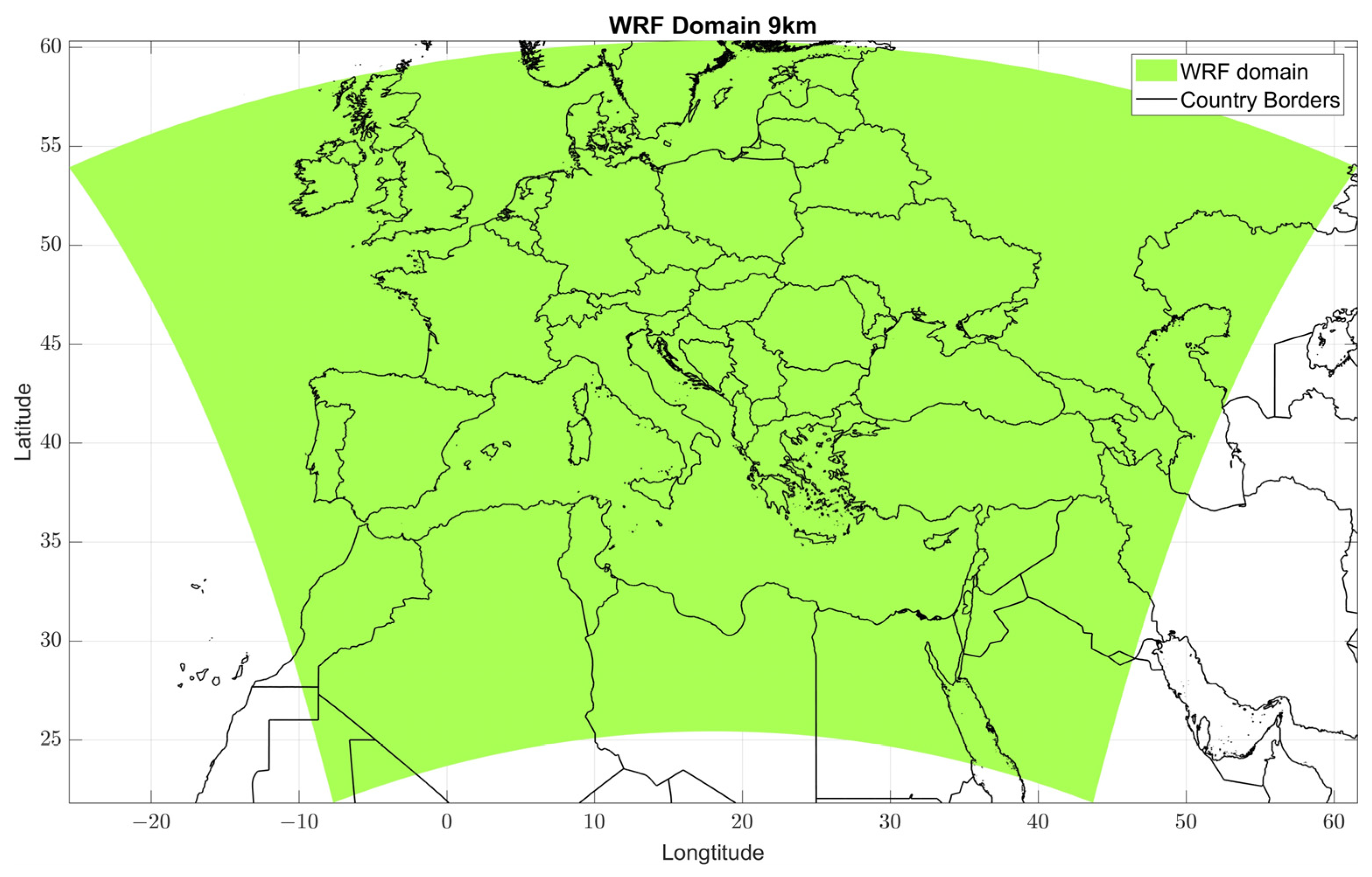
Significant meteorological activity is observed in the Mediterranean and especially in the Balkans, a region of Europe with intense and damaging weather events such as heavy rainfall, heavy thunderstorms, and convective supercells. As a result, the impact on the coastal communities in the region is major, causing widespread damage, flooding, and disruption to transportation and other essential services. The experimental design consists of a single domain covering South Europe, including the Mediterranean Sea (Figure 2), which has 620 × 440 horizontal mesh grids with 9 km spacing and 60 vertical levels up to 50 hPa. The projection method is Lambert. In the model integration, the coordinates of the central point are 42.894° N and 18.025° E. The spatial scale of this case’s supercell had a frontal line that extended in a range of 210 km to 250 km, with a core diameter of 70 km, showing that a 9 km grid size is sufficient to resolve it.

4.3. Parametrization Schemes in WRF

The WRF model provides options for different physical parameterizations, including microphysics, cumulus physics, surface physics, planetary boundary layer physics, and radiation physics. The model’s performance is highly dependent on the parameterization schemes, which might be suitable for one storm event but inappropriate for others.

For this reason, the parameterization schemes remained fixed for the convective simulations that were analyzed. More specifically, the main physics packages used in this study include the WRF Single-Moment 6-class microphysical parameterization, the Rapid Radiative Transfer Model (RRTM) shortwave and longwave radiation scheme, Mellor–Yamada–Janjic (MYJ) planetary boundary layer scheme, Tiedtke scheme for cumulus parameterization, and Monin–Obukhov-based surface layer (Eta similarity), as part of studies for convective weather conditions as well as complex terrain configurations [43].

4.4. Sources and Types of Observations

The observations used in this first attempt to apply and assess DA schemes for ameliorating the forecasts of such complex cases included only GTS METAR observations data during the month of July 2019. The surface data assimilated in this study are obtained from HNMS archives, which contain measurements of pressure, geopotential height, temperature, dew point temperature, wind direction, and speed from fixed land stations. A total of 312 multi-national observation stations have been gathered (Figure 3). The availability of the data at each time frame determines the specific time slots in which the corresponding observations are accessible. Observations that fall within a window of +30 min to −29 min relative to each hour are considered valid for assimilation. This approach creates hourly sets of observations. Satellite radiances, as well as other indirect observations, are not used in this study. The observation preprocessing module (OBSPROC) of WRF VAR is implemented for data sorting, quality control, and observational error assignment [32]. The data are initially downloaded in ASCII format and cannot be assimilated directly into WRFDA. A conversion from ASCII to LITLE_R format was performed in order to be ingested into the WRF VAR system. Estimated precipitation was also used from integrated multi-satellite retrievals for GPM (IMERG) [44] at a grid spacing of 0.1 degrees to evaluate the total precipitation. Finally, lightning data from the network of the Hellenic National Meteorological Service (HNMS) were used to show the impact and intensity of this frontal activity (not shown).

4.5. Initial Conditions for Model Runs

Gridded analyses and forecast data were obtained from the operational archive of the deterministic model from the European Centre for Medium-Range Weather Forecasts (ECMWF) in order to use the initial and boundary conditions necessary to run the WRF. The data were retrieved in the region extending from 20° N to 62° N and from 30° W to 65° E. The ECMWF deterministic forecast system is an atmosphere-only, full-physics, hydrostatic model, and its output is disseminated on a 0.1° lat. × 0.1° long. grid. The analysis fields were available at 3-h intervals from 00 UTC 1.07.2018 to 00 UTC 20.07.2018 and from 00 UTC 10.07.2019 to 00 UTC 12.07.2019. The data were retrieved on the surface level and on the pressure levels of 1000, 950, 925, 850, 800, 700, 600, 500, 400, 300, 250, 200, 150, and 100 hPa.

5. Results

In this section, the steps of model applications and the corresponding DA efforts are outlined. An initial run is performed to establish a baseline configuration. Following this, the process and significance of modeling the BE covariance, commonly known as the B matrix, is explained, followed by the techniques and datasets utilized in our DA phase. The outcomes and deviations observed post DA are evaluated, as well as the impact and improvements over the initial runs.

5.1. Initial Run

An initial run for a period of two days was performed, which will serve as initial conditions for a warm start after data assimilation. The run is from 10.07.2019 00:00 UTC to 12.07.2019 00:00 UTC. Trying to overcome spin-up issues, the forecast of 06:00 UTC of 10.07.2019 was selected for DA purposes as a warm start, and the assimilated initial conditions are used for the runs of WRF after the DA of surface observation, performed for CV5, CV6, and CV7 configurations, starting from 10.07.2019 06:00 UTC to 12.07.2019 00:00 UTC.

5.2. Background Error Covariance Analysis

The BE covariance in 3D-VAR experiments is static and prescribed by the NMC method [20]. It assumes homogeneous and isotropic correlations for a set of independent control variables derived from the forecast differences. In this study, the CV5, CV6, and CV7 options are used.

For the evaluation of BE, a 20-day period starting from 1.07.2018 to 20.07.2018 was selected. Forecasts of 12 h and 24 h WRF-ARW outputs, initialized both at 00:00 and at 12:00 UTC, were used. Thus, 40 pairs of perturbations are available to generate WRF-ARW BE. The test case examined refers to July of 2019, but the statistics refer to a year prior to the test case, based on the assumption that at the time when the event occurred, no statistical data were available. Thus, a climatological approach is to use the previous year’s data.

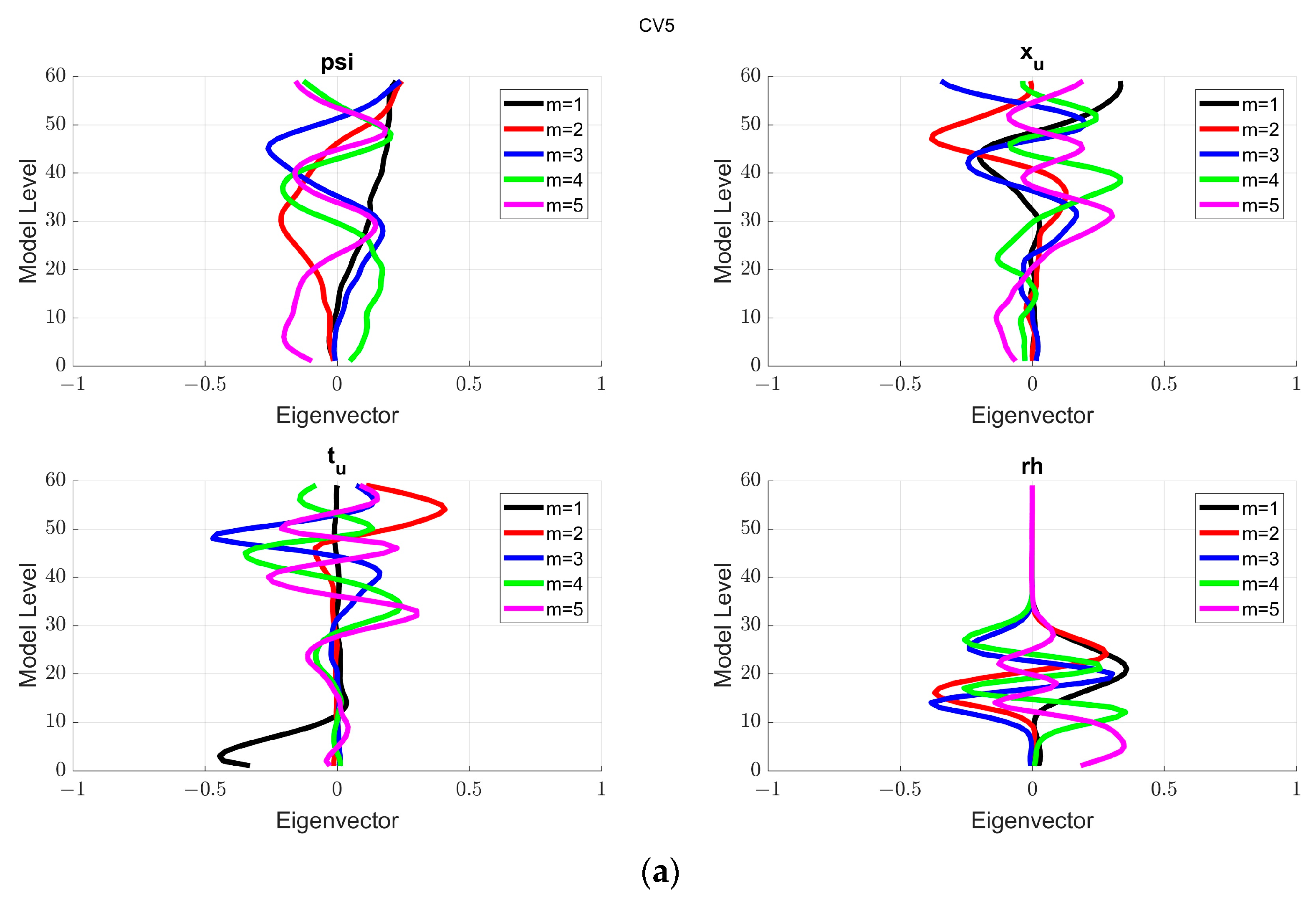
The reliability of DA significantly hinges on the accurate representation of the BE covariance B. Analyzing the eigenvectors corresponding to each configuration provides an enriched understanding of the role that various atmospheric variables play in influencing the overall error statistics.

For the CV5 configuration, the eigenstructure of the BE was analyzed across the five eigenvectors for each variable. As seen in Figure 4a, the y axis represents the levels resolved by the model, and the x axis has the first five eigenvalues of each eigenvector. Regarding relative humidity (rh) at the first eigenvector, large-scale error structures associated become evident, exhibiting broad spatial structures across the model domain, potentially pointing to persistent atmospheric circulations or model biases. The values of streamfunction (ψ) in the first eigenvector reveal the interconnected nature of dynamic and thermodynamic processes in the atmosphere. Analyzing the rest of them, the atmospheric dynamics manifest in more complex patterns, indicating the intricate variability of streamfunction. The temperature (t_u) pattern suggests a growth in the lower levels, while the rh pattern suggests an interaction up to the intermediate levels. However, studying the rest of the eigenvectors, the relation grows more intricate, emphasizing the dynamic influence of temperature on the atmospheric structure.

For the CV6 configuration (Figure 4b), the eigenstructure was again dissected across the first five modes. The oscillatory patterns in rh grow more pronounced, suggesting a rich interplay at intermediate scales. The patterns in ψ and χ are the same as the CV5 configuration. The values of t_u highlight a dynamic equilibrium between temperature and other constituents, pivotal for the determination of moisture levels and circulation patterns.

For the CV7 configuration (Figure 4c), the patterns in rh are the same as the CV5 configuration. The temperature patterns in CV7 also suggest variabilities like CV6 configuration.

5.3. Background Error Length Scales Analysis

A configuration overview regarding the control variable options follows; option CV5 consistently leans toward broader, synoptic scales across all the variables. This configuration is likely to be more relevant for large-scale weather events and phenomena, having a representation in the broader, synoptic scales. CV6, on the other hand, has been consistent in its representation of more localized mesoscale processes. It would be instrumental in understanding and predicting more localized weather events, especially in complex terrains or regions with significant land–sea interactions or convective events. CV7 is a transitional configuration and leans toward microscale phenomena, whereas its behavior is between synoptic-scale and mesoscale phenomena. The above length scales are derived from the BE covariance matrices for each CV configuration.

Analyzing ψ variable (available for CV5 and CV6 options), the length scales for CV5 start at broader values and tend to decrease steadily across levels, indicating a more synoptic behavior and representation. CV6 has generally smaller length scales compared to CV5, implying a more mesoscale and localized behavior.

Analyzing the χ variable (available for CV5 and CV6), the CV5 configuration exhibits larger spatial correlations with length scales showcasing steady declines across levels, reflecting the broader scales. For the CV6 configuration, as with ψ, a more localized behavior is displayed, with smaller length scales across levels.

Regarding the t variable (temperature for all configurations: CV5, CV6, and CV7) (Figure 5), for the CV5 configuration, we encounter larger length scales to start with, gradually reducing across levels. This suggests broader spatial correlations in the beginning. CV6 exhibits smaller length scales throughout compared to CV5, showcasing its typical mesoscale behavior. CV7 displays a transitional behavior between CV5 and CV6, so we might expect length scales somewhere in between the two, striking a balance between synoptic and mesoscale characteristics. However, if CV7 leans more toward microscale representations, the length scales might be smaller than both CV5 and CV6.

Finally, for the rh variable (relative humidity), CV5 and CV7 options have the same length scales, while CV6 exhibits similar patterns.

Incorporating these insights can greatly optimize model utilization for specific weather prediction needs. For broader weather patterns, CV5 would be the most suitable. For more localized predictions, CV6 seems to be the most appropriate. Depending on the wind accuracy necessity, CV7 could be used for both mesoscale or synoptic area simulations, where the wind is the most important variable for assimilation.

5.4. Data Assimilation Using CV5, CV6, and CV7

DA of surface observation was performed for CV5, CV6, and CV7 BE. The variance scale parameter is carefully tuned to 3.0 rather than the default value of 1.0 to provide the best performance of the 3D-VAR among various experiments tested (not shown; this also improves the performance of 4D-VAR as compared to the default) [3].

As stated in Section 5.1, the initial conditions for DA and the new runs refer to 06:00 UTC of 10.07.2019. Three DA processes were performed for the three different BE configurations previously examined, using the same set of observations, as stated in 4.4. The process of DA for each control variable option is shown in Figure 6.

The minimization of the cost function, as assessed using the conjugate gradient (CG) method, was performed across three different CV configurations: CV5, CV6, and CV7. All three configurations started from an identical cost function value of 2923.71. The initial gradients were different, with CV5, CV6, and CV7 showing initial gradients of 60.35, 55.10, and 87.87, respectively. This indicates that the CV7 setup had the steepest gradient, implying the most substantial deviation from the minimum.

CV5 took 12 iterations to converge to a cost function of 2379.51, showing a reduction of 544.2 from its initial value. CV6 converged in 10 iterations to a value of 2462.67, a decrease of 461.04. CV7 required the most iterations (16) to converge to a cost function of 1841.01, marking a significant reduction of 1082.7. As iterations progress, the gradient values for all configurations diminish. CV7 demonstrated the largest initial gradient, but it also showed the steepest decline, highlighting rapid convergence, especially in the first few iterations. For all configurations, the step sizes were not uniform, fluctuating based on the gradient magnitude and the curvature of the cost function.

Among the configurations, CV5 and CV6 required fewer iterations compared to CV7. However, CV7 achieved a more substantial reduction in the cost function value despite the necessity of more iterations. CV7 converged to the lowest cost function value of the three, indicating a better fit for the given problem.

The final J/(total number of observations) value for CV7 is also the lowest, suggesting that, on average, the misfit between observations and the model field is the smallest for CV7. However, CV7 required a few more iterations to converge compared to CV5 and CV6. The selection of the best option should consider other factors as well, such as computational efficiency and the physical interpretation of the results.

Table 2. Evaluation of objective functions across different CV options.

CV Option	Final Value of J	Final Value of Jo	Final Value of Jb
CV5	2379.51	2146.56	232.95
CV6	2462.67	2279.39	183.29
CV7	1841.01	1418.01	423.01

details the computed outcomes of the objective function J for various CV configurations, namely CV5, CV6, and CV7. The final value of J is segmented into observational (J_o) and background (J_b) components. CV7 stands out with the lowest overall value of J, whereas CV6 stands out with the lowest value of J_b.

The calculation of the background term J_b, as well as the calculation of the observation term J_o, based on $\mathrm{J}\left(\mathrm{v}\right)={\mathrm{J}}_{\mathrm{b}}+{\mathrm{J}}_0$ (Equation (2)), shows that CV6 has the lowest value of J_o, followed by CV5 and then CV7. Having as criteria the J_b value and not the J value, CV6 exhibited the best performance based on the results. The contribution of Jo in the final J value of CV6 is the biggest compared to CV5 and CV7, and this serves as observations that are well fitted to the analysis field much more efficiently than the other two CVs.

5.5. Runs and Analysis Post Data Assimilation

Three sets of new forecasts were available after the DA process. As the starting time was 06:00 UTC of 10.07.2019, the simulation of the WRF-ARW was performed for 42 h up to 00:00 UTC of 12.7.2019. The original run, which started at 00:00 UTC of 10.07.2019, will be referred to as ORIG, RCV5 for the run after CV5 option BE DA, RCV6 for the run after CV6 option BE DA, and RCV7 for the run after CV7 option BE DA.

Discrepancies are evident among these forecasts, necessitating detailed evaluation. This enhancement is sought through the exclusive use of one kind of observation (surface METAR), thereby enabling an assessment of the control variables. Given the sole reliance on surface observations, the contrasts among ORIG, RCV5, RCV6, and RCV7 manifest close to the surface of the model. This justifies the emphasis on near-surface and surface-layer discrepancies in our presentation.

In order to evaluate the results, a simple linear regression analysis between the surface observations and the CV results was performed, and the corresponding R², slope, and RMSE values were calculated. In particular, the verification was between the observational data and forecasts for each ORIG, RCV5, RCV6, and RCV7.

Table 3. Slope of regression between IMERG data vs. different runs.

Slope
	ORIG	RCV5	RCV6	RCV7
10.07.2019 09:00 UTC	0.574596407	0.579820502	0.591004545	0.580909283
10.07.2019 12:00 UTC	0.528259375	0.530443518	0.536777983	0.530303622
10.07.2019 15:00 UTC	0.541017141	0.545911233	0.547654013	0.547349451
11.07.2019 00:00 UTC	0.763604456	0.764116932	0.770858861	0.765469658
11.07.2019 18:00 UTC	0.617027986	0.618871979	0.61865578	0.61854543
11.07.2019 21:00 UTC	0.722005614	0.72469613	0.72496216	0.723679649
12.07.2019 00:00 UTC	0.755929304	0.757677061	0.756957918	0.758342565

illustrates the results for specific humidity parameters in periods with sufficient data available. The dates presented in Table 3,

Table 4. RMSE of regression between IMERG data vs. different runs.

$\mathbf{RMSE} ({10}^{-3} \mathbf{g} \times \mathbf{k}{\mathbf{g}}^{-1})$
	ORIG	RCV5	RCV6	RCV7
10.07.2019 09:00 UTC	2.939403097	2.906229779	2.790401193	2.901062785
10.07.2019 12:00 UTC	2.99862999	2.978911749	2.931584172	2.976548541
10.07.2019 15:00 UTC	2.415220807	2.371456968	2.389589067	2.374596434
11.07.2019 00:00 UTC	2.396224849	2.38678574	2.358999465	2.389230651
11.07.2019 18:00 UTC	3.151521169	3.144182149	3.142446493	3.13495034
11.07.2019 21:00 UTC	2.623882552	2.612348846	2.619757037	2.613839418
12.07.2019 00:00 UTC	2.34083961	2.348286227	2.341523816	2.339594189

and

Table 5. IMERG observations versus runs.

24 h Total Precipitation
CV	ORIG	RCV5	RCV6	RCV7
Slope	0.2326	0.2316	0.2488	0.2337
RMSE (mm)	9.0845	9.0700	9.1989	9.4180
R-square	0.3093	0.3044	0.3469	0.2917

were chosen in order to have sufficient data samples for verification, as there were collection issues of archives where intermediate hours were faulty. The linear regression between the observations and the forecasts over the entire set of observations for the whole domain indicated that CV6 configuration forecasts (RCV6 run) had the best fit, as the higher values of the slope. Table 4 further supports this outcome, showing the RCV6 runs to have the lowest RMSE among most of the runs.

CV6 configuration has a direct effect on representing humidity correlation, and this makes it the best configuration among these three for convective phenomena simulations. It is also noticeable that the ORIG run had the worst score compared with runs in which data assimilation was performed.

The above results are further supported when comparing IMERG and forecasted 24 h precipitation in an area that affected Greece the most, encompassing the Balkans (Figure 7 Area A). The scattered diagrams between IMERG and forecast (not shown) indicate that there are both overestimation and underestimation of the observation. However, applying a simple regression analysis on these data, it is indicated that the slope and the R-square for RCV6 are the largest among the runs, and the RMSE has a minimum value for RCV5 (Table 5).

Trying to support the result of the more accurate convective role of CV6 configuration, an area near Chalkidiki was selected to narrow down the results (Figure 7—Area B). The same comparison was made between IMERG and forecasted 24 h precipitation, as shown in

Table 6. IMERG observations versus CV and original run (small).

24 h Total Precipitation
CV	ORIG	RCV5	RCV6	RCV7
Slope	0.2822	0.2629	0.2988	0.277
RMSE (mm)	15.5242	16.0893	15.3334	16.5668
R-square	0.1100	0.0088	0.2337	0.0598

, where the slope and the R-square of RCV6 are the biggest, and the RMSE has the lowest value among the runs as well.

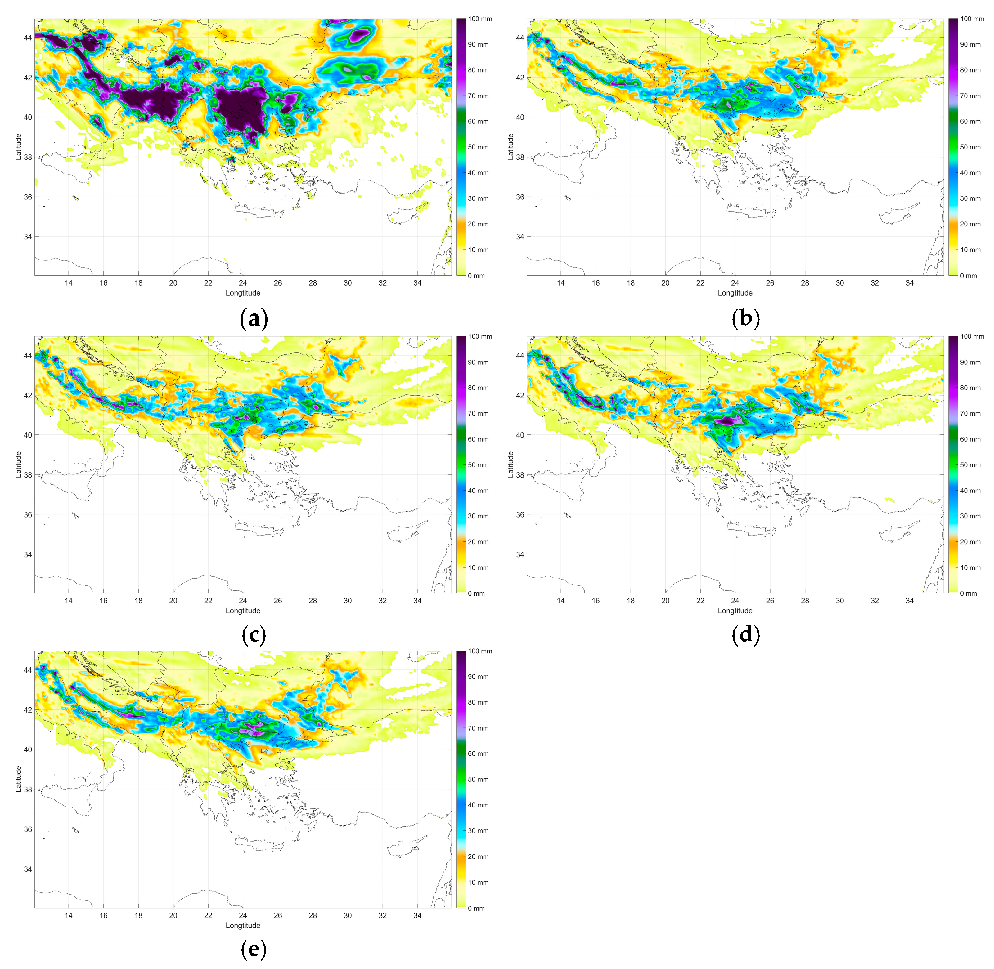
It is evident across all model outputs that the IMERG data (Figure 8a) showcased higher precipitation values compared to the runs ORIG, RCV5, RCV6, and RCV7. This visual comparative analysis offers insights into how the assimilation of surface observations under different CV configurations affects model outcomes as well as the mathematical approach. Among all model runs, ORIG consistently demonstrated the least intensity of precipitation over the Chalkidiki area (Figure 8b). This suggests the possibility that the initial conditions in ORIG might not capture certain atmospheric features or mechanisms driving precipitation over the region. The RCV5 run visualized in Figure 8c reveals an increase in precipitation intensity over Chalkidiki compared to ORIG. However, this increase remains notably subdued when compared to the IMERG data and the other assimilation runs. The CV5 assimilation seems to have added some fidelity to the model over ORIG but is not as aggressive as CV6 in its precipitation forecast. Figure 8d, showcasing the CV6 BE DA scenario, presents the most intense precipitation forecast over Chalkidiki among all runs. The amplification suggests that the assimilation of data in the CV6 scenario has a pronounced effect on the model’s prediction of mesoscale convective systems or similar rain-producing mechanisms over the region. The RCV7 run, illustrated in Figure 8e, while showcasing a significant increase in precipitation, especially in the northern regions of Greece, places its intensity somewhere between CV5 and CV6 for the Chalkidiki area. This spatial variation indicates that CV7 may be capturing different atmospheric dynamics or processes that are more influential toward the northern parts of Greece as a local phenomenon due to wind direction increments.

In summary, while all model runs after the assimilation of surface observations (RCV5, RCV6, and RCV7) produced higher precipitation values than ORIG, they all remained conservative when compared to IMERG estimates, which serve as a reference for precipitation patterns in areas where rain gauge data are not available. This suggests that while DA can enhance the model’s accuracy, there is still a discrepancy between model forecasts and observed data, hinting at other influencing factors and the need for the inclusion of additional observational datasets. As stated before, the scope of this study is to underline the best practice regarding convection and probably capturing supercell intensity, such as this test case studied, especially when orography evidently plays a crucial role in forecasting regarding complex terrain. The findings underscore the value of DA in refining NWP model outputs. However, they also emphasize the necessity for continuous model evaluation and adjustment to better align with observational data.

6. Conclusions

In this study, surface data assimilation (DA) is implemented in WRF DA 3D-VAR and applied to a 9 km model configuration. We studied three control variable configurations, namely CV5, CV6, and CV7, to incorporate climatological background errors (Bes) utilizing the NMC method in WRF VAR. The DA fields were evaluated with a focus on understanding the impact of ΒΕ on convective weather evolution under complex terrain. Utilizing the WRF model, different BEs were calculated and compared to show their effects on the resulting weather forecasts.

The CVs were tested for simulating the convective weather conditions in a supercell case over a complex terrain configuration, a study which, to the knowledge of the authors, is the first time to be performed over Greece. In this way, insights are gained in their usage regarding the resolving space scales. The results suggest that the representation of BE plays a pivotal role in VAR DA. Specifically, the WRF runs demonstrate how different BE can influence weather evolution. It is clear that BE covariance calculation greatly influences the reliability of DA processes and, hence, the NWPs by influencing processes at different scales, such as cloud formation, vertical convective motions, and overall precipitation dynamics, especially regarding convection. Our findings illustrate that the CV6 configuration is a suitable approach for data assimilation regarding supercell thunderstorm forecasting, accommodating local-scale effects induced by orography as well as mesoscale characteristics.

Directly comparing the WRF runs of ORIG (no DA), RCV5, RCV6, and RCV7, it was evident that the latter three, post-DA runs, showcased an overall improvement in forecast accuracy over the Chalkidiki area regarding precipitation amounts. Among these, CV6 emerged as the standout, making the configuration CV6 an optimal choice for weather prediction in scenarios where localized phenomena develop, such as convective weather events. Configuration for CV6 had the minimum value of J_b, and the produced run, namely RCV6 forecasts, were enriched with the most rain gauge values while notably influencing the weather evolution, having the biggest amount of precipitation over the Chalkidiki region, and the highest score in the forecasts when validated to surface observations of humidity among RCV5, RCV7, and ORIG runs. Such an alignment of CV6 with localized mesoscale processes suggests that the representation of BE, especially those closely adhering to ground observations, can considerably affect the accuracy of NWP and DA mechanisms. This indicates that when our BE aligns closely with observations, our weather forecasting accuracy improves significantly, as shown by the minimization of the J_b term of Equation (2). Hence, CV6 seems to perform better in resolving the necessary scales associated with the extreme and complex convective event, producing more accurate precipitation forecasts, although only METAR observations were taken into account in the DA.

This study emphasizes how the selection of background error (BE) can notably improve humidity parameters, which are critical for convection phenomena. This fine tuning in data assimilation provides new insights into the significance of control variable configurations for enhancing the reliability of weather forecasting. The horizontal length scale was analyzed in order to describe to what extent the horizontal background covariance can spread the observation information. Given the limited availability of quality data in certain regions for DA, BE reliability is highly important. Furthermore, BE reliability becomes crucial, especially where the orography is quite complex and peculiarities of locally developed weather phenomena at any time in the year are often characterized by diversity and extremity, such as supercell thunderstorms. This study explores the novelty of the role of different control variable configurations in weather forecasting within the context of Greece’s notably complex terrain.

Different BE statistics experiments may be further applied for better fine tuning in the performance of WRFs’ forecasting ability, as in this study, the primary source of observational input for DA stemmed from surface METAR observations only. While surface observations are integral to refining the lower atmospheric layers and boundary conditions of the model, they have inherent limitations as they provide data on near-ground conditions and primarily influence the boundary layer conditions in model simulations. While they can provide valuable insights into atmospheric variables near the ground, they do not offer a holistic understanding of the entire atmospheric column. Therefore, incorporating upper-air observations, whether direct or indirect, could offer a more comprehensive depiction of atmospheric dynamics. Satellite-derived measurements, radiosonde data, and aircraft observations can provide insights into mid-tropospheric and upper-tropospheric conditions.

Having a more diverse observation dataset has the potential to improve forecasting skills using observations that are not only surface based but in the upper atmosphere layers as well. Radar data assimilation emerges as a promising solution for future research, as radar data offer high-resolution, three-dimensional insights into precipitation structures and dynamics. Integrating radar-derived observations could drastically enhance the accuracy of precipitation forecasts, especially for localized and intense meteorological events, influencing cloud dynamics and precipitation by diversifying the observational datasets integrated into the model—spanning from the surface to the upper atmosphere—where lies the potential for substantially improved and more accurate NWP outputs. Successful modeling of the BE covariance matrix is a prerequisite for further development of the NWP system in any regional NWP with DA.

References

- Scorer, R.S. Atmospheric data analysis, Roger Daley, Cambridge Atmospheric and Space Science Series, Cambridge University Press, Cambridge, 1991. No. of pages: Xiv + 457. Price: £55–00, US$79–50 (hardback) ISBN 0521 382157. Int. J. Climatol. 1992, 12, 763–764. [Google Scholar] [CrossRef]
- Bannister, R.N. A review of forecast error covariance statistics in atmospheric variational data assimilation. I: Characteristics and measurements of forecast error covariances. Q. J. R. Meteorol. Soc. 2008, 134, 1951–1970. [Google Scholar] [CrossRef]
- Zhang, M.; Zhang, F.; Huang, X.-Y.; Zhang, X. Intercomparison of an Ensemble Kalman Filter with Three- and Four-Dimensional Variational Data Assimilation Methods in a Limited-Area Model over the Month of June 2003. Mon. Weather Rev. 2011, 139, 566–572. [Google Scholar] [CrossRef]
- Lindskog, M.; Gustafsson, N.; Mogensen, K.S. Representation of background error standard deviations in a limited area model data assimilation system. Tellus A Dyn. Meteorol. Oceanogr. 2006, 58, 430. [Google Scholar] [CrossRef]
- Hacker, J.P.; Rostkier-Edelstein, D. PBL state estimation with surface observations, a column model, and an ensemble filter. Mon. Weather Rev. 2007, 135, 2958–2972. [Google Scholar] [CrossRef]
- Stensrud, D.J.; Yussouf, N.; Dowell, D.C.; Coniglio, M.C. Assimilating surface data into a mesoscale model ensemble: Cold pool analyses from spring 2007. Atmos. Res. 2009, 93, 207–220. [Google Scholar] [CrossRef]
- Bauer, P.; Lopez, P.; Benedetti, A.; Salmond, D.; Moreau, E. Implementation of 1D + 4DVAR assimilation of precipitation affected microwave radiances at ECMWF. I: 1D-Var. Q. J. R. Meteorol. Soc. 2006, 132, 2277–2306. [Google Scholar] [CrossRef]
- Bauer, P.; Lopez, P.; Salmond, D.; Benedetti, A.; Saarinen, S.; Bonazzola, M. Implementation of 1D+4DVAR assimilation of precipitation-affected microwave radiances at ECMWF. II: 4DVAR. Q. J. R. Meteorol. Soc. 2006, 132, 2307–2332. [Google Scholar] [CrossRef]
- Bauer, P.; Geer, A.J.; Lopez, P.; Salmond, D. Direct 4DVAR assimilation of all-sky radiances. Part I. Implementation. Q. J. R. Meteorol. Soc. 2010, 136, 1868–1885. [Google Scholar] [CrossRef]
- Geer, A.J.; Bauer, P.; Lopez, P. Direct 4DVAR assimilation of all-sky radiances. Part II: Assessment. Q. J. R. Meteorol. Soc. 2010, 136, 1886–1905. [Google Scholar] [CrossRef]
- Sokol, Z.; Rezacova, D. Assimilation of radar reflectivity into the LMCOSMO model with a high horizontal resolution. Meteorol. Appl. 2006, 13, 317–330. [Google Scholar] [CrossRef]
- Sokol, Z. Assimilation of extrapolated radar reflectivity into a NWP model and its impact on a precipitation forecast at high resolution. Atmos. Res. 2011, 100, 201–212. [Google Scholar] [CrossRef]
- Wang, H.; Sun, J.; Fan, S.; Huang, X.-Y. Indirect Assimilation of Radar Reflectivity with WRF 3D-Var and Its Impact on Prediction of Four Summertime Convective Events. J. Appl. Meteorol. Clim. 2013, 52, 889–902. [Google Scholar] [CrossRef]
- Macpherson, B. Operational experience with assimilation of rainfall data in the Met Office mesoscale model. Meteorol. Atmos. Phys. 2001, 76, 3–8. [Google Scholar] [CrossRef]
- Stephan, K.; Klink, S.; Schraff, C. Assimilation of radar-derived rain rates into the convective-scale model COSMO-DE at DWD. Q. J. R. Meteorol. Soc. 2008, 134, 1315–1326. [Google Scholar] [CrossRef]
- Alapaty, K.; Niyogi, D.; Chen, F.; Pyle, P.; Chandrasekar, A.; Seaman, N. Development of the Flux-Adjusting Surface Data Assimilation System for Mesoscale Models. J. Appl. Meteorol. Climatol. 2008, 47, 2331–2350. [Google Scholar] [CrossRef]
- Ruggiero, F.H.; Modica, G.D.; Lipton, A.E. Assimilation of Satellite Imager Data and Surface Observations to Improve Analysis of Circulations Forced by Cloud Shading Contrasts. Mon. Weather Rev. 2000, 128, 434. [Google Scholar] [CrossRef]
- Wang, H.; Huang, X.-Y.; Xu, D.; Liu, J. A scale-dependent blending scheme for WRFDA: Impact on regional weather forecasting. Geosci. Model Dev. 2014, 7, 1819–1828. [Google Scholar] [CrossRef]
- Hollingsworth, A.; Shaw, D.B.; Lönnberg, P.; Illari, L.; Arpe, K.; Simmons, A.J. Monitoring of Observation and Analysis Quality by a Data Assimilation System. Mon. Weather Rev. 1986, 114, 861–879. [Google Scholar] [CrossRef]
- Parrish, D.F.; Derber, J.C. The National Meteorological Center’s Spectral Statistical-Interpolation Analysis System. Mon. Weather Rev. 1992, 120, 1747–1763. [Google Scholar] [CrossRef]
- Bouttier, E. Application of Kalman filtering to numerical weather prediction. In Proceedings of the 1996 ECMWF Seminar on Data Assimilation, Reading, UK, 2–6 September 1996; pp. 61–90. [Google Scholar]
- Houtekamer, P.L.; Mitchell, H.L. A sequential ensemble Kalman filter for atmospheric data assimilation. J. Geophys. Res. Atmos. 1998, 103, 32251–32270. [Google Scholar] [CrossRef]
- Dee, D.P.; Uppala, S.M.; Simmons, A.J.; Berrisford, P.; Poli, P.; Kobayashi, S.; Andrae, U.; Balmaseda, M.A.; Balsamo, G.; Bauer, P.; et al. The ERA-Interim reanalysis: Configuration and performance of the data assimilation system. Q. J. R. Meteorol. Soc. 2011, 137, 553–597. [Google Scholar] [CrossRef]
- Kutaladze, N.; Mikuchadze, G. Background Error in WRF Model. WSEAS Trans. Environ. Dev. 2020, 16, 619–624. [Google Scholar] [CrossRef]
- Gustafsson, N.; Janjić, T.; Schraff, C.; Leuenberger, D.; Weissmann, M.; Reich, H.; Brousseau, P.; Montmerle, T.; Wattrelot, E.; Bučánek, A.; et al. Survey of data assimilation methods for convective-scale numerical weather prediction at operational centres. Q. J. R. Meteorol. Soc. 2018, 144, 1218–1256. [Google Scholar] [CrossRef]
- Lee, J.C.K.; Huang, X. Background error statistics in the Tropics: Structures and impact in a convective-scale numerical weather prediction system. Q. J. R. Meteorol. Soc. 2020, 146, 2154–2173. [Google Scholar] [CrossRef]
- Emmanouil, S.; Langousis, A.; Nikolopoulos, E.I.; Anagnostou, E.N. The Spatiotemporal Evolution of Rainfall Extremes in a Changing Climate: A CONUS-Wide Assessment Based on Multifractal Scaling Arguments. Earth’s Future 2022, 10, e2021EF002539. [Google Scholar] [CrossRef]
- Emmanouil, S.; Langousis, A.; Nikolopoulos, E.I.; Anagnostou, E.N. Exploring the Future of Rainfall Extremes Over CONUS: The Effects of High Emission Climate Change Trajectories on the Intensity and Frequency of Rare Precipitation Events. Earth’s Future 2023, 11, e2022EF003039. [Google Scholar] [CrossRef]
- Lopez-Cantu, T.; Prein, A.F.; Samaras, C. Uncertainties in Future U.S. Extreme Precipitation from Downscaled Climate Projections. Geophys. Res. Lett. 2020, 47, e2019GL086797. [Google Scholar] [CrossRef]
- Moustakis, Y.; Papalexiou, S.M.; Onof, C.J.; Paschalis, A. Seasonality, Intensity, and Duration of Rainfall Extremes Change in a Warmer Climate. Earth’s Future 2021, 9, e2020EF001824. [Google Scholar] [CrossRef]
- Prein, A.F.; Mearns, L.O.U.S. Extreme Precipitation Weather Types Increased in Frequency During the 20th Century. J. Geophys. Res. Atmos. 2021, 126. [Google Scholar] [CrossRef]
- Barker, D.M.; Huang, W.; Guo, Y.-R.; Bourgeois, A.J.; Xiao, Q.N. A Three-Dimensional Variational Data Assimilation System for MM5: Implementation and Initial Results. Mon. Weather Rev. 2004, 132, 897–914. [Google Scholar] [CrossRef]
- Federico, S. Implementation of a 3D-Var system for atmospheric profiling data assimilation into the RAMS model: Initial results. Atmos. Meas. Tech. 2013, 6, 3563–3576. [Google Scholar] [CrossRef]
- Courtier, P.; Talagrand, O.; Anderson, J.L.; Gauthier, E. A proposal for the operational implementation of the three-dimensional variational analysis (3DVAR). Q. J. R. Meteorol. Soc. 1994, 120, 1367–1387. [Google Scholar]
- Hayden, C.M.; Purser, R.J. Recursive Filter Objective Analysis of Meteorological Fields: Applications to NESDIS Operational Processing. J. Appl. Meteorol. 1995, 34, 3–15. [Google Scholar] [CrossRef]
- Purser, R.J.; Wu, W.-S.; Parrish, D.F.; Roberts, N.M. Numerical aspects of the application of recursive filters to variational statistical analysis. Part I: Spatially homogeneous and isotropic Gaussian covariances. Mon. Weather Rev. 2003, 131, 1524–1535. [Google Scholar] [CrossRef]
- Chen, Y.; Rizvi, S.R.; Huang, X.-Y.; Min, J.; Zhang, X. Balance characteristics of multivariate background error covariances and their impact on analyses and forecasts in tropical and Arctic regions. Meteorol. Atmos. Phys. 2013, 121, 79–98. [Google Scholar] [CrossRef]
- Wang, H.; Huang, X.-Y.; Sun, J.; Xu, D.; Zhang, M.; Fan, S.; Zhong, J. Inhomogeneous Background Error Modeling for WRF-Var Using the NMC Method. J. Appl. Meteorol. Climatol. 2014, 53, 2287–2309. [Google Scholar] [CrossRef]
- Sun, J.; Wang, H.; Tong, W.; Zhang, Y.; Lin, C.-Y.; Xu, D. Comparison of the Impacts of Momentum Control Variables on High-Resolution Variational Data Assimilation and Precipitation Forecasting. Mon. Weather Rev. 2016, 144, 149–169. [Google Scholar] [CrossRef]
- Skolnik, M.I. Radar Handbook, 3rd ed.; McGraw-Hill: New York, NY, USA, 2008; ISBN 978-0-07-148547-0. [Google Scholar]
- Sugimoto, S.; Crook, N.A.; Sun, J.; Xiao, Q.; Barker, D.M. An Examination of WRF 3DVAR Radar Data Assimilation on Its Capability in Retrieving Unobserved Variables and Forecasting Precipitation through Observing System Simulation Experiments. Mon. Weather Rev. 2009, 137, 4011–4029. [Google Scholar] [CrossRef]
- Skamarock, W.C.; Klemp, J.B.; Dudhia, J.; Gill, D.O.; Liu, Z.; Berner, J.; Huang, X. A Description of the Advanced Research WRF Model Version 4.3; No. NCAR/TN-556+STR; National Center for Atmospheric Research: Boulder, CO, USA, 2021. [Google Scholar] [CrossRef]
- Mukherjee, S.; Lohani, P.; Tiwari, A.; Sturman, A. Impacts of terrain on convective surface layer turbulence over central Himalaya based on Monin–Obukhov similarity theory. J. Atmos. Sol.-Terr. Phys. 2021, 225, 105748. [Google Scholar] [CrossRef]
- Girotto, M.; Huffman, G.J.; Habib, E. The integrated multi-satellite retrievals for GPM (IMERG) early science-The GPM era of global precipitation estimates. Earth Space Sci. 2017, 4, 314–327. [Google Scholar]
Figure 1.
(a) Surface pressure chart analysis of Europe for 09.07.2019 12:00 UTC, (b) Chalkidiki area and Thessaloniki radar maximum dBz for 10.07.2019 at 18:47 UTC.
Figure 2.
Domain used for WRF simulations.
Figure 3.
Surface observations used in the Europe area for DA.
Figure 4.
Five eigenvectors for (a) CV5 (ψ, xu, tu, and rh variables), (b) CV6 (ψ, xu, tu, and rhu variables), and (c) CV7 (u, v, tu, and rh variables).
Figure 5.
Length scale analysis for (a) CV5 (ψ, xu, tu and rh variables), (b) CV6 (ψ, xu, tu and rhu variables), and (c) CV7 (tu variable). Blue lines: ψ, red: xu, magenta: rh and green: tu.
Figure 6.
Cost function convergence analysis. A comparative plot showcasing the cost function J values across different iterations for each of the CVs. The figure illustrates the efficiency of the minimization process within the DA for CV5, CV6, and CV7, highlighting the relative convergence patterns and the optimization dynamics of each CV.
Figure 7.
Areas for comparison—Areas A and B.
Figure 8.
The 24 h accumulated precipitation during 10.07.2019 06:00 UTC to 11.07.2019 06:00 UTC covering Greece (a) as estimated by the IMERG dataset, (b) forecasted by the original model (ORIG) without DA, (c) forecast post DA in the CV5 BE DA scenario, (d) forecast post DA in the CV6 BE DA scenario, and (e) forecast post DA in the CV7 BE DA setup.