
Identification of Pollution Sources in Urban Wind Environments Using the Regularized Residual Method

1
Tianmushan Laboratory, Yuhang District, Hangzhou 311115, China
2
College of Urban Construction, Nanjing Tech University, Nanjing 211816, China
3
Institute of Industrial Science, The University of Tokyo, 4-6-1 Komaba, Meguro-ku, Tokyo 153-8505, Japan
4
School of Aeronautic Science and Engineering, Beihang University, Beijing 100191, China
*
Author to whom correspondence should be addressed.
Atmosphere 2023, 14(12), 1786; https://0-doi-org.brum.beds.ac.uk/10.3390/atmos14121786
Submission received: 1 November 2023
/
Revised: 28 November 2023
/
Accepted: 30 November 2023
/
Published: 4 December 2023
(This article belongs to the Special Issue Exposure to Indoor CO2 and Human Response)
Abstract
:The scale of cities is increasing with continuous urban development. Effective methods, such as the source term estimation (STE) method, must be established for identifying the sources of air pollution in cities to prevent economic losses and casualties caused by pollutant leakage. Herein, methods for optimizing sensor configuration and identifying pollution sources are discussed, and an STE method based on the regularized minimum residual method is proposed. Urban wind environments were simulated using a computational fluid dynamics (CFD) model, and the results were compared with experimental data pertaining to the wind tunnel of an architectural ensemble to verify the model’s accuracy. The sensor layout was optimized using the simulated annealing (SA) algorithm and adjoint entropy, and the relationship between sensor responses and potential pollution sources was established using the CFD model. Pollutant concentrations measured using sensors were combined with the regularization method to extrapolate the pollution source strength, and the regularized minimum residual method was used to obtain the locations of the real pollution sources. The results show that compared with the Bayesian methods, the proposed method can more accurately identify pollution sources (100%), with a smaller source strength error of 2.01% for constant sources and one of 2.62% for attenuation sources.
1. Introduction
Air quality and urban wind environments are crucial to the health of urban inhabitants [1], and pollutants released from vehicles and industrial parks are the main air pollution sources [2]. With the continuous increase in the scale of urban and industrial production, when harmful gas leakage occurs in cities or industrial parks, the ability to trace pollution sources in a timely manner is of great significance for providing early warnings regarding disasters and post-disaster emergency rescue. In recent years, several harmful gas emission accidents have caused great damage to society. For example, the air pollution caused by the radioactive substances discharged by the Fukushima Daiichi nuclear power plant after the Tohoku earthquake and tsunami nuclear accident on 11 March 2011 led to huge economic losses. On 8 October 2015, Williams Natural Gas Pipeline Transportation Company in Houma Town, Louisiana, USA, suffered a pipeline leak [3,4]. Most of these harmful gas leakage accidents caused huge economic losses and social panic. In addition, due to the spread of harmful gases, if the leakage source of harmful gases is not discovered in time, relevant management departments or enterprises will not be able to quickly control the spread of pollutants, and the evacuation of surrounding people will also be delayed. The lives and health of the residents around a leakage accident are seriously threatened, with the resulting danger even affecting the stability of society. Therefore, it is important to establish optimal monitoring networks and accurately estimate the parameters of a leakage source.
Several studies [5,6] have used uniform or random sensor configurations, which yielded poor-quality data and inaccurate inverse identification results for the source parameters. Therefore, Keats et al. [7] proposed an information-based experimental design method to solve the optimal design problem by increasing the number of sensors used to measure the source information. Their method could effectively solve the optimal design problem, and suggested optimization algorithms that maximize the objective function will be required for future sensor arrangements. Keats et al.’s method [7] can save sensor resources by selecting an optimal sensor network for maximizing the objective function using an optimization algorithm. Liu et al. [8] used computational fluid dynamics (CFD) to analyze the effect of sensor layout on source term estimation (STE) performance and suggested an optimal sensor layout for measuring air pollutants in urban agglomerations. They analyzed the effects of source position and the boundary effects of the measurement point on STE performance. Ngae [9] optimized the deployment of sensor and mobile networks in emergency situations by coupling CFD adjoint fields, renormalization algorithms, and simulated annealing (SA) algorithms to evaluate the sensitivity of sensors in urban areas in order to reconstruct unknown source information. Himanshu et al. [10] developed a linear transfer Perron–Frobenius (P–F) operator framework based on dynamic systems to analyze and solve design problems in building systems. Jia et al. [11] proposed a sensor configuration optimization (SCO) method composed of an objective function and an SA algorithm for identifying an optimum sensor configuration that can provide informative concentration measurements for STE, regardless of where the unknown source appears in the target domain. These reported studies effectively optimized sensor networks using diverse methods.
Information on pollution sources is obtained using the probability method based on Bayesian and optimization methods. The predicted results obtained using these methods are then compared with observed data to determine an ideal method for STE. For Bayesian method, Waeytens et al. [12] used an adjoint model to determine the observable region associated with sensor positions and used the Bayesian method to identify the pollution source. Pudykiewicz [13] used the adjoint source–receptor relationship to estimate a single source term and achieved good estimation results. Xue et al. [14] proposed a two-step deterministic method for deriving the analytical form of the marginal a posteriori probability density function for estimating the source position. This method needs prior information and poses complexity for multi-parameter searches. For the optimization method, Sharan et al. [15] proposed a new two-step optimization algorithm that used least-squares data assimilation for skip initialization and identifying single- and multipoint release sources in a limited number of atmospheric concentration measurements. However, the least-squares optimization method is not a global optimization technique and largely relies on good initial estimates; otherwise, its use can result in a local minimum. Allen et al. [16] used a genetic algorithm (GA) to estimate the two-dimensional position, intensity, and surface wind direction of pollutant sources to determine their information. Annunzi et al. [17] combined GAs with adjoint methods to obtain accurate pollutant-source information. Thomson et al. [18] used an SA algorithm to generate candidate distributions of source strength and position and evaluated these distributions using cost functions to determine the true source information. These studies addressed the shortcomings of the least-squares method and employed algorithms such as GAs and SAs to optimize the search for the optimal solution. Bayesian and optimization methods are often combined for STE. First, the optimization method and sensor data are used to calculate the source strength. Subsequently, the Bayesian method and sensor data are used to calculate the a posteriori probability of the source position. This method involves complex calculations and may yield low-accuracy results due to some of the sensor data used in each step.
Therefore, in this paper, we propose a new method for calculating unknown potential source position and source strength, namely, the minimum regularization residual method, to replace the complex calculation of likelihood functions and posterior probability required by the Bayesian method. Compared with previous methods, the minimum regularization residual method has the following advantages:
- (1)
- Compared with calculating a posteriori probability to infer source position, the implementation steps of the minimum regularization residual method are more concise and can save calculation time;
- (2)
- The regularized minimum residual method uses all the response sensor data to calculate the source strength and uses its calculation residual to calculate the source position, and the calculation results are more accurate.
In Section 2, this paper will introduce the principle of the minimum regularization residual method for source term estimation (Section 2.1), including a case study of urban buildings and the arrangement of sensors and potential pollution sources (Section 2.2). In Section 3, the most unfavorable potential source is selected as a simulation case, and its position and release source strength are calculated and compared with those for the traditional Bayesian method. Finally, Section 4 introduces the conclusions drawn from this study.
2. Material and Methods
2.1. Algorithm for Identifying the Pollution Source
When the flow field of gaseous pollutants released in the spatiotemporal domain is stabilized, a linear relationship exists between the source release rate q and concentration C of the pollutants at the monitoring point. This relation can be expressed as follows:
The matrix is shown below:
where represents the concentration response vector that describes the relationship between concentration and release rate, while and represent the response factor of the computational region with respect to the sensor position and the ith time step, respectively. The information on pollution sources in urban agglomerations can be analyzed based on the response vectors between potential sources and sensors.
Based on the linear relationship established by the response vectors and the pollutant-source concentration monitored using the sensors, inverse calculation can be used to derive the pollutant release intensity. The inverse computation of the matrix is an ill-posed process that requires regularization methods for maintaining the values of the solution within a certain range to reduce its oscillation or instability. Therefore, two regularization methods—the Tikhonov regularization method, which introduces a regularization parameter to improve inverse operation stability, and the iterative regularization method, which uses iterative computations such that the solution discretely converges to an appropriate value—are used herein to solve the inverse inference problem. The Tikhonov regularization formula is as follows:
where and represent the regularization matrix and the Tikhonov regularization parameter, respectively. The selection of an appropriate regularization parameter is crucial to accurately derive the release intensity of the pollution sources, and the Generalized Cross Validation (GCV) method is relatively stable compared to other methods in terms of the selection of regularization parameters [19]. The GCV method is used to perform minimum generalized cross-validation of the discrete regularization parameters to obtain the smooth parameter , which can be expressed as follows:
represents the matrix that generates the regularization solution . Furthermore, the source release intensity is calculated using singular value decomposition based on the monitored pollutant concentration.
The Simultaneous Multiplicative Algebraic Reconstruction Technique (SMART) and least squares using QR factorization (LSQR) algorithms are classical iterative regularization methods. The SMART [20] algorithm is an algebraic iterative method used to accelerate the convergence of computing large quantities of data. Its principle is represented as follows:
where represents the number of iterations, represents the th element of the source strength vector , represents the element in the matrix , and represents the element in the pollutant-concentration sequence .
The LSQR algorithm, which is a well-established iterative algorithm based on a diagonalization process [21], generates the sequence with monotonically decreasing residual paradigms, similar to that generated by the standard CG algorithm and other algorithms. When the response matrix is large or sparse, the LSQR algorithm is numerically more reliable and yields more accurate solutions in fewer iterations.
In this study, multiple sensors with concentration responses are used to back-calculate the source strength, and the regularized minimum residual method is used instead of the complex likelihood probability function to determine the source position. In particular, the source strength calculated using the regularization algorithm is incorporated into Equation (5) to calculate the residuals of each unknown source position. By comparing the residuals of each potential source, the potential source with the smallest residual is determined to be the position of the real source. This approach uses more concise calculation and analysis steps and satisfies the conditions for obtaining an optimal solution under the over-determined constraint.
Here, represents the position residual of the potential pollutant source. The performance of this approach was compared with that based on the Bayesian method. The details can be found in Jing et al.’s work [22]. They used these three regularization methods to compute the source information. First, the source–receptor response relationship was calculated using the adjoint method. Then, a single sensor was used to estimate the source strength inversely based on the source–receptor response relation. Finally, the other sensors were used to analyze the a posteriori probability of each potential source and identify the real source location.
Simultaneously, the error between the simulated and actual source strengths was calculated as follows:
where represents the source strength error, represents the number of time steps detected by the sensor, represents the simulated source strength for time steps, and represents the experimental source strength. A smaller source strength error implies that the estimated and actual source strength are quite consistent.
2.2. Simulation of Urban Architectural Ensembles and Sensor Placement
CFD is mainly used for studying urban environments due to its technological advancements compared to traditional methods such as on-site measurements and (semi) empirical models [23,24]. Therefore, the CFD method was used herein to simulate the street environment in cities to obtain the concentration data. Then, the concentration data were used to identify the source term inversely based on the proposed STE method. The wind tunnel experimental data of urban buildings from the Architectural Institute of Japan (AIJ) [25] were used for simulation verification (Figure 1). This is an ideal urban-scale model for studying the diffusion of atmospheric pollutants. The dense distribution of building blocks in the model will cause turbulent and laminar mixed flow patterns, such as separation and wake vortices, which can be used to verify the STE and sensor placement. Herein, only a single wind direction consistent with the experimental data was used for verification analysis.
2.2.1. Simulation Settings for Urban Architectural Ensembles
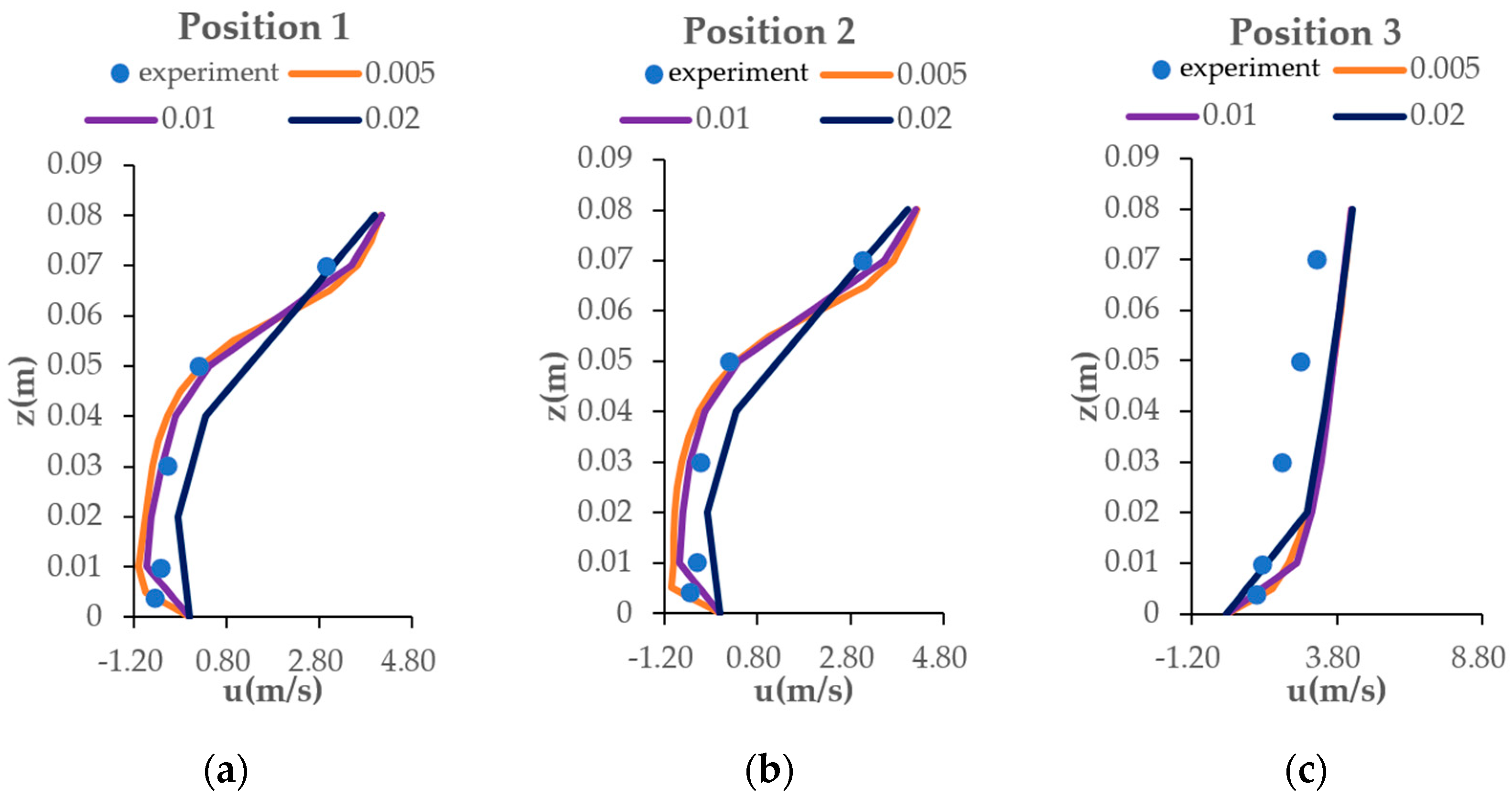
The computational domain of the building complex is 16H × 14H × 4H (where H is the height of the building, 0.06 m), as shown in Figure 1; this domain can be used to capture the complete statistical information of the flow field [26]. For the CFD computational grid, three grid sizes, 0.02, 0.01, and 0.005 m, were compared (Figure 2); the results changed less when the grid size was increased to 0.005 m. Thus, a homogeneous grid of 0.01 m in size was selected for simulation herein based on the output of the grid independence test. The pollutant outlet is an urban square, with the outlet side length set to 0.02 m. It is located on the ground in the recirculation area of the building, 0.02 m away from the leeward wall of the building, and the pollutant-release intensity is m3/s. A turbulent Schmidt number (Sct) of 0.3 was set, because conventional modeling with Sct = 0.3 yielded results similar to the experimental results [27].
Alongside a comparison with the k-ε and large eddy simulation model [28], the shear stress transport (SST) k-ω turbulence model was used in this study; it is fast and suitable for gentle and curvature flow, vortex shedding flow, and boundary layer separation flow, and these types of flow are in line with the characteristics of the simulated urban environment [29]. The SIMPLE algorithm was used to solve the pressure–velocity coupling equation [30], and the second-order upwind scheme was used as the variable discretization scheme. In terms of boundary conditions, the inlet wind speed profile was set based on the actual wind speed profile from the wind tunnel experiment. In addition, the vertical distribution of turbulent kinetic energy k(z) was obtained by fitting the wind tunnel experimental data. The turbulent kinetic dissipation rate is expressed following the recommendations of AIJ:
where = 0.09 represents the model constant.
Figure 3 compares the CFD simulation data with the normalized velocity, turbulent kinetic energy, and pollutant-concentration data from the wind tunnel experiment (normalized parameters are velocity, turbulent kinetic energy, and concentration measured at the corresponding position of 0.03 m (H/2)). The flow field and concentration field were determined for the cross-section of the wake area of the buildings, where the pollutants are released in accordance with y = 7H (Figure 1).
2.2.2. Potential Pollution Sources and Sensor Layout
Previous studies [5,6] on sensor configuration used random or manual methods to determine the influence of different sensor configurations on measurement results, yielding poor-quality data and inaccurate back-calculations of the source parameters. Considering the characteristics of the case presented in Section 2.2.1, the sensor network selection method proposed by Jia et al. [11] is used here, and the information entropy of the sensor network was set as the objective function to evaluate the sensor configuration efficiency. The information entropy of the probability distribution [31] is defined as follows:
A narrow distribution with a sharp peak has lower entropy, whereas a wide distribution with a slight slope has greater entropy. Therefore, a uniform distribution has maximum entropy [32]. For a system of n sensors, the corresponding entropy of the associated concentration field R with respect to the background information I is as follows:
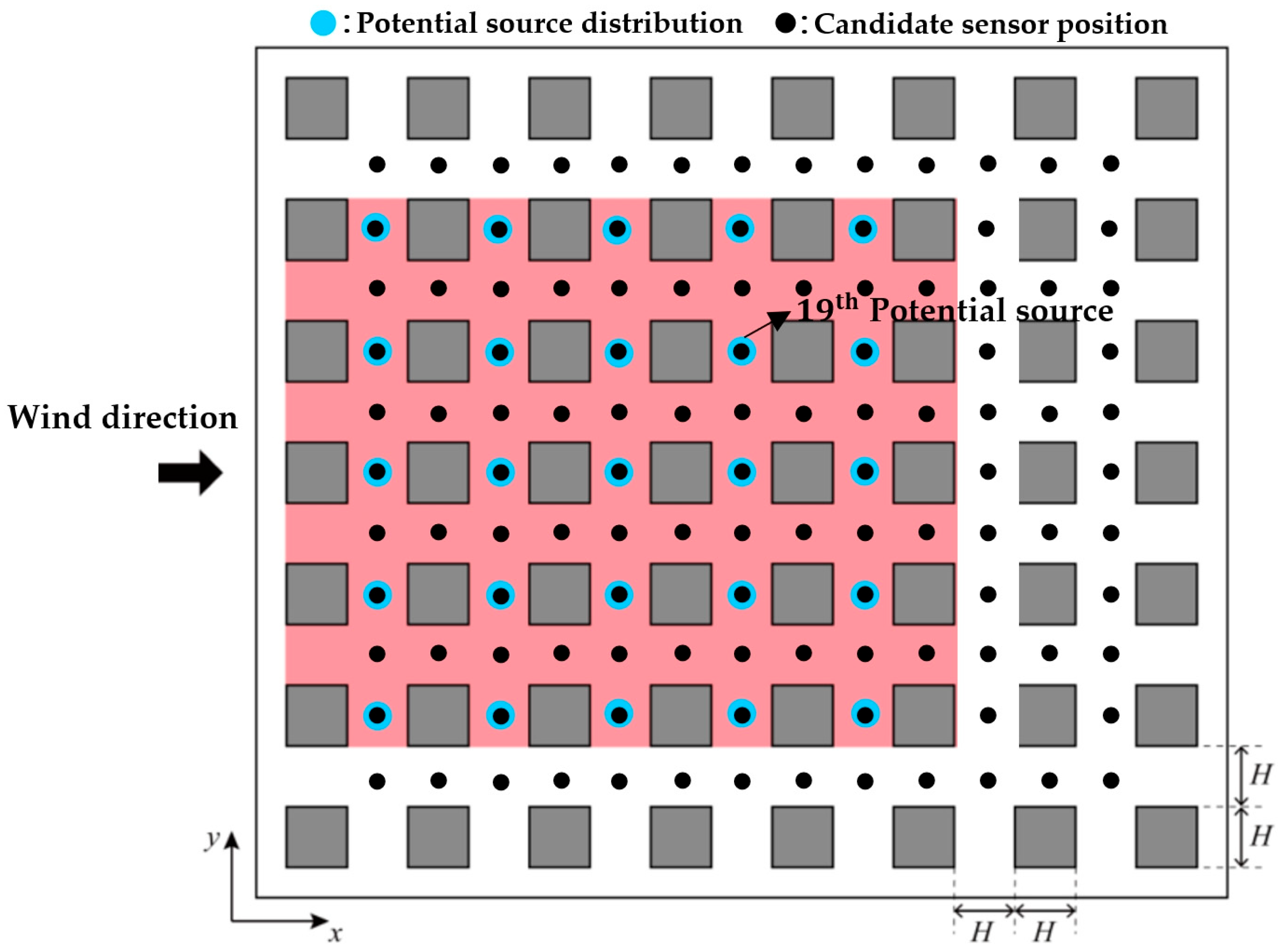
where represents the probability of the spatial distribution of the concentration field in the target area. In general, the ideal effective measurement area of the sensor can cover each potential source (on average) (Figure 4). Based on the analysis of the factors influencing the above entropy values, multiple sensors will widen the spatial probability distribution and increase the corresponding information entropy compared to a single sensor. However, the number of sensors cannot be indefinitely increased to make the process economical. The information entropy can be increased by optimizing the sensor topology, thereby increasing the probability of successfully identifying the real source. Herein, random nonrepetitive sampling and an SA algorithm are used in conjunction to verify the independence of different numbers of sensors. Using as the objective function, the optimal sensor network that can identify potential pollution sources is calculated when the number of sensors is 4, 8, and 12 (the sensors are selected from candidate sensors, as shown in Figure 4).
The red region in Figure 4 represents the primary distribution area of potential sources. It is worth noting that all of these sources are located in the middle of the wake region, where there is strong unsteady turbulence flow. This can better challenge and validate the proposed STE method across different sensor configurations.
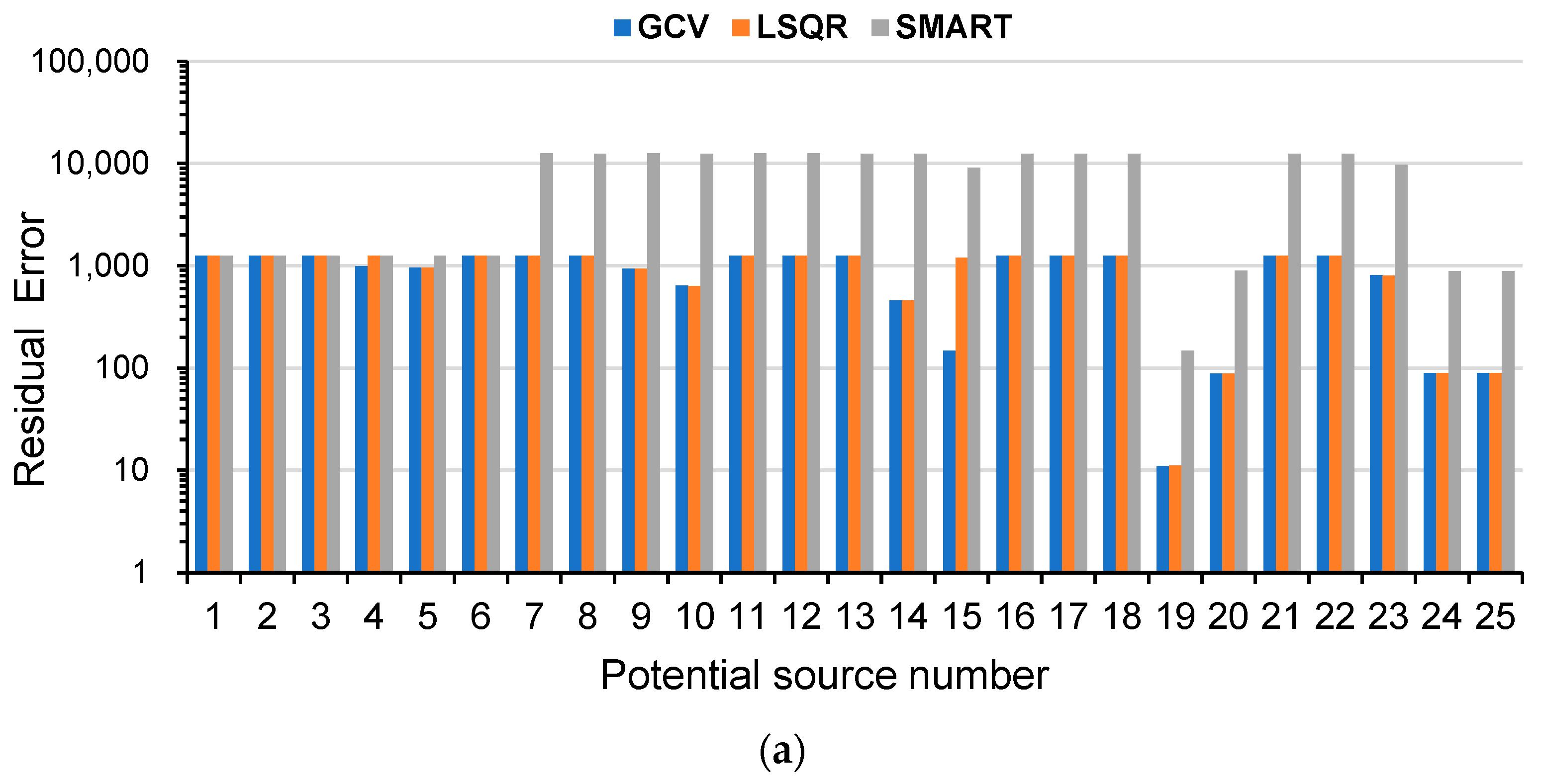
After the number and arrangement of sensors were determined, potential source #19 in the downstream region of the airflow was selected from among the 25 potential locations to show the identification of the source item using the regularized minimum residual method below. First, the response sensor readings were used to determine the source strength; Equation (6) was used to calculate the residuals of each potential source position to determine the source location. In addition, the effectiveness of regularization methods, mainly GCV, LSQR, and SMART, in identifying two source types, constant and attenuation sources, was determined by comparing the results with the method that uses the Bayesian criterion.
3. Results
3.1. Independent Verification of the Number of Sensors
An ideal sensor arrangement is a prerequisite for correctly identifying a pollution source. Based on the sensor placement discussed in Section 2.2.2, the number of sensors was independently verified for the urban architectural ensemble model (Section 2.2.1). In addition, the efficiency of different quantities of sensors (4, 8, and 12) in identifying potential pollution sources was determined. The release intensity of pollution source 1 kg/(m3·s) was considered.
Figure 5 illustrates the iterative process of the SA chains, and the optimal layouts of 4, 8, and 12 sensors were determined when the information entropy reached its maximum values and stabilized. Figure 6 shows the sensor layouts obtained using the SA and adjoint entropy algorithm with different quantities of sensors and the predicted results regarding the source strengths and locations of the pollution sources. Figure 6 shows that the 25 potential pollutant sources in the urban architectural ensemble model were all identified using 8 and 12 sensors, whereas two potential locations could not be identified when 4 sensors were used. When the number of sensors was changed from 4 to 8, the average recognition error for the 25 source strengths was reduced from 8.64% to 2.92%, which is a major improvement in calculation accuracy. When the number of sensors was changed from 8 to 12, the error reduction was not significant. Therefore, eight sensors were chosen for sensor optimization and pollution source identification to make the process economical.
3.2. Identification Results for the Regularized Minimum Residual Method
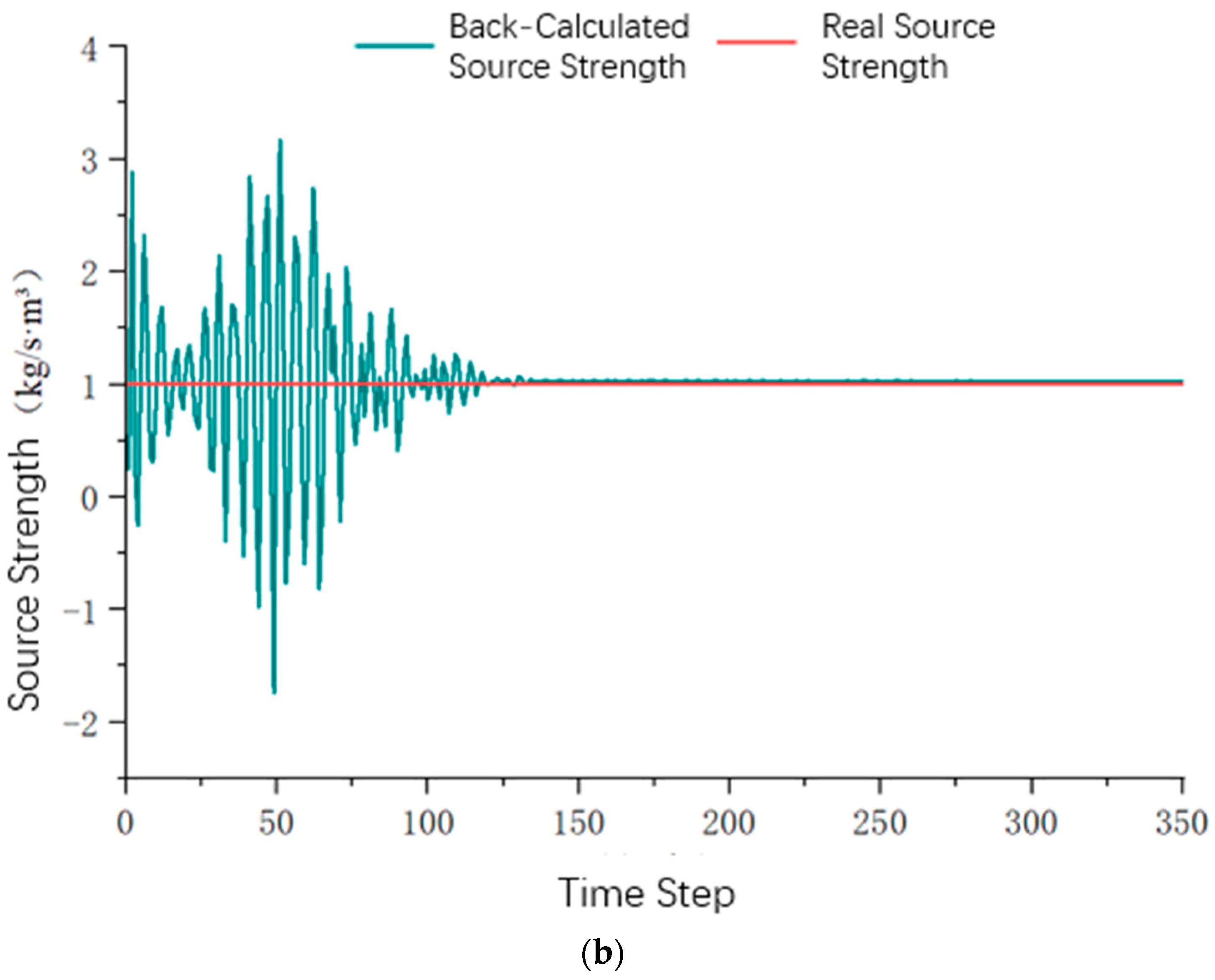
Figure 7 shows the source strength and residual calculation results for potential source #19. This source was located at the downstream off-edge position. The residuals of constant source #19 are smaller than those of the other potential sources; i.e., the regularized minimum residual method is effective in identifying the position of the real source, as shown in Figure 7a. Figure 7b shows that the real source strength obtained from the inverse calculation is very close to the actual source strength, and the average errors of the three regularization algorithms, GCV, LSQR, and SMART, are 2.72%, 6.59%, and 2.01%, respectively.
The regularized minimum residual method can also be used to identify the location of an attenuation source (Figure 8b), and the inverse predicted source strength is very close to the source strength transmitted by the actual source. The average errors obtained using GCV, LSQR, and SMART were 2.84%, 6.57%, and 2.62%, respectively. These results show that the regularized minimum residual method can be used to effectively identify the locations of different pollution sources. Moreover, SMART is the best regularization algorithm, whereas the LSQR algorithm yields a larger error.
3.3. Comparative Analysis with Bayesian Method
Section 3.2 discussed the inverse calculation of potential source #19. In this section, the location of the same source was used as the constant pollutant-release point, and, due to the accuracy of the SMART algorithm mentioned above, the SMART regularization algorithm was used. The results from the regularized minimum residual method were compared with the computational results obtained using the Bayesian criterion method to verify their performance. Figure 9a shows the a posteriori probabilities of different potential source locations calculated using the Bayesian criterion. The a posteriori probabilities of source #19 and source #9 are the same, and the real source locations cannot be identified. Figure 9b shows that the inverse calculated source strength is 21.09%, which is higher than the source strength error (2.01%) computed using the regularized minimum residual method.
4. Discussion
The comparison of the aforementioned source strengths shows that the regularized residual method yields more accurate results than the Bayesian method. Identifying attenuation sources is more difficult than identifying constant sources; thus, the Bayesian method may not yield accurate results, and no further calculations and comparisons were made in this study. The regularized minimum residual method performs better mainly because it uses all the sensor data to invert the source strength and determine the source location. Contrarily, the Bayesian method uses a portion of the sensor data to invert the source strength and search for the source location.
In the context of real urban blocks or industrial parks, buildings of different heights distributed on a non-regular lattice [33] and the presence of multiple sources of pollution may be prevalent. For multi-source release, an algorithm is required initially to detect the number of pollution sources. Furthermore, the potential combinations of multiple pollution sources are significantly more extensive than those of single sources. Therefore, an optimized sampling algorithm is also needed. In addition, the distribution of potential sources, as depicted in Figure 4, exhibits a relatively sparse arrangement. As a result, there may be deviations in the position and intensity of the actual pollution source parameters compared to the calculated values. These aspects necessitate further research in the future.
5. Conclusions
For the identification of pollution source locations and source intensity in urban wind environments, we proposed the minimum regularization residual method, which simplifies the calculation steps and improves identification accuracy. Specifically, in the verified CFD model, the sensor optimization algorithm was used to independently verify the number of sensors, and the positioning and intensity reverse calculations of constant and attenuation sources released at different locations were performed based on the optimized sensor structure. At the same time, the constant source was taken as an example, and the method based on Bayes criterion was compared. The main conclusions are as follows:
- (1)
- Through the optimization calculation of different quantities of sensor networks, it was found that eight sensors can meet the needs of pollution source item identification for the example used herein.
- (2)
- The minimization residual method proposed in this study can be used to identify the source strengths and locations of potential sources in a city model. Using the calculation of constant sources and attenuation sources, the error of source strength identification is about 2%, and the location can be accurately identified.
- (3)
- Compared with the traditional method based on Bayes criterion, the minimization residual method utilizes the response information of multiple response sensors; this information is more accurate for the inverse calculation of source strength and more intuitive and accurate for position calculation.
Author Contributions
Conceptualization, F.L. and X.C.; methodology, S.T. and X.X.; validation, X.X.; formal analysis, S.T.; resources, X.C. and H.J.; writing—original draft preparation, X.X. and S.T.; writing—review and editing, F.L. and H.J.; visualization, Z.G.; supervision, F.L. and X.C. All authors have read and agreed to the published version of the manuscript.
Funding
This research was financially supported by the National Natural Science Foundation of China (Grant No. 52008014), the Postgraduate Research & Practice Innovation Program of Jiangsu Province (Grant No. SJCX23_0492), and the Fundamental Research Funds for the Central Universities (YWF-23-SDHK-L-013).
Institutional Review Board Statement
Not applicable.
Informed Consent Statement
Not applicable.
Data Availability Statement
The data that support the findings of this study are available from the corresponding author upon reasonable request. This research was financially supported by the National Natural Science Foundation of China. In accordance with the regulations governing the management of research outcomes funded by the National Natural Science Foundation, the corresponding author is not entitled to publicly disclose the data associated with this research paper.
Conflicts of Interest
The authors declare no conflict of interest.
References
- Zhou, P.; Wang, H.; Li, F.; Dai, Y.; Huang, C. Development of window opening models for residential building in hot summer and cold winter climate zone of China. Energy Built Environ. 2022, 3, 363–372. [Google Scholar]
- Ming, T.; Nie, C.; Li, W.; Kang, X.; Wu, Y.; Zhang, M.; Peng, C. Numerical study of reactive pollutants diffusion in urban street canyons with a viaduct. Build. Simul. 2022, 15, 1227–1241. [Google Scholar]
- Morino, Y.; Ohara, T.; Masato, N. Atmospheric behavior, deposition, and budget of radioactive materials from the Fukushima Daiichi nuclear power plant in March 2011. Geophys. Res. Lett. 2011, 38, L00G11. [Google Scholar]
- U.S. EPA. EPA Strategic Plan; U.S. EPA: Washington, DC, USA, 2014. [Google Scholar]
- Li, F.; Zhuang, J.; Li, M.; Cai, H.; Zhang, J.; Cao, X. Reconstruction of airflow path parameters in multizone models based on Bayesian inference and measured data. Build. Environ. 2022, 209, 108689. [Google Scholar]
- Keats, A.; Yee, E.; Lien, F.S. Bayesian inference for source determination with applications to a complex urban environment. Atmos. Environ. 2007, 41, 465–479. [Google Scholar]
- Keats, A.; Yee, E.; Lien, F.S. Information-driven receptor placement for contaminant source determination. Environ. Model. Softw. 2010, 25, 1000–1013. [Google Scholar]
- Liu, Z.Z.; Li, X.F. The impact of sensor layout on Source Term Estimation in urban neighborhood. Build. Environ. 2016, 213, 108859. [Google Scholar]
- Ngae, P.; Kouichi, H.; Kumar, P.; Feiz, A.C. Optimization of Urban Monitoring Network for Emergency Response Applications: An Approach for Characterising Source of Hazardous Releases, LMEE, Université d’Evry V al-d’Essonne. Q. J. R. Meteorol. Society 2019, 145, 967–981. [Google Scholar]
- Himanshu, S.; Anthony, D.F.; Umesh, V.; Baskar, G. Transfer Operator Theoretic Framework for Monitoring Building Indoor Environment in Uncertain Operating Conditions. In Proceedings of the Annua American Control Conference, Milwaukee, WI, USA, 27–29 June 2018. [Google Scholar]
- Jia, H.Y.; Kikumoto, H. Sensor configuration optimization based on the entropy of adjoint concentration distribution for stochastic source term estimation in urban environment. Sustain. Cities Soc. 2022, 79, 103726. [Google Scholar]
- Waeytens, J.; Sadr, S. Computer-aided placement of air quality sensors using adjoint framework and sensor features to localize indoor source emission. Build. Environ. 2018, 144, 184–193. [Google Scholar]
- Pudykiewicz, J.A. Application of adjoint tracer transport equations for evaluating source parameters. Atmos. Environ. 1998, 32, 3039–3050. [Google Scholar]
- Xue, F.; Li, X.F.; Ooka, R.; Kikumoto, H.; Zhang, W. Turbulent Schmidt number for source term estimation using Bayesian inference. Build. Environ. 2017, 125, 414–422. [Google Scholar]
- Sharan, M.; Singh, S.K.; Issartel, J.P. Least Square Data Assimilation for Identification of the Point Source Emissions. Pure Appl. Geophys. 2012, 169, 483–497. [Google Scholar]
- Allen, C.T.; Haupt, S.E.; Young, G.S. Source characterization with a genetic algorithm-coupled dispersion-backward model incorporating scipuff. J. Appl. Meteorol. Clim. 2007, 46, 273–287. [Google Scholar]
- Annunzio, A.J.; Young, G.S.; Haupt, S.E. Utilizing state estimation to determine the source location for a contaminant. Atmos. Environ. 2012, 46, 580–589. [Google Scholar]
- Thomson, L.C.; Hirst, B.; Gibson, G.; Gillespie, S.; Jonathan, P.; Skeldon, K.D.; Padgett, M.J. An improved algorithm for locating a gas source using inverse methods. Atmos. Environ. 2007, 41, 1128–1134. [Google Scholar]
- Kim, Y.J.; Gu, C. Smoothing spline Gaussian regression: More scalable computation via efficient approximation. J. R. Stat. Soc. Ser. B (Stat. Methodol.) 2004, 66, 337–356. [Google Scholar]
- Jeon, M.G.; Deguchi, Y.; Kamimoto, T.; Doh, D.H.; Cho, G.R. Performances of new reconstruction algorithms for CT-TDLAS (computer tomography-tunable diode laser absorption spectroscopy). Appl. Therm. Eng. 2017, 115, 1148–1160. [Google Scholar]
- Paige, C.C.; Saunders, M.A. LSQR: An algorithm for sparse linear equations and sparse least squares. ACM Trans. Math. Softw. (TOMS) 1982, 8, 43–71. [Google Scholar]
- Jing, Y.; Li, F.; Gu, Z.; Tang, S. Identifying spatiotemporal information of the point pollutant source indoors based on the adjoint-regularization method. Build. Simul. 2013, 16, 589–602. [Google Scholar]
- Yoshihide, T.; Ted, S. CFD simulations of near-field pollutant dispersion with different plume buoyancies. Build. Environ. 2018, 131, 128–139. [Google Scholar]
- Beatriz, S.; Jose Luis, S.; Alberto, M.; Magdalena, P.; Lourdes, N.; Manuel, P.; Jaime, F. NOx depolluting performance of photocatalytic materials in an urban area–Part II: Assessment through Computational Fluid Dynamics simulations. Atmos. Environ. 2021, 246, 118091. [Google Scholar]
- Tominaga, Y.; Mochida, A.; Yoshie, R.; Kataoka, H.; Nozu, T.; Yoshikawa, M.; Shirasawa, T. AIJ guidelines for practical applications of CFD to pedestrian wind environment around buildings. J. Wind Eng. Ind. Aerodyn. 2008, 96, 1749–1761. [Google Scholar]
- Coceal, O.; Thomas, T.G.; Castro, I.P.; Belcher, S.E. Mean flow and turbulence statistics over groups of urban-like cubical obstacles. Bound. -Layer Meteorol. 2006, 121, 491–519. [Google Scholar]
- Lin, C.; Ooka, R.; Kikumoto, H.; Jia, H. Eulerian RANS simulations of near-field pollutant dispersion around buildings using concentration diffusivity limiter with travel time. Build. Environ. 2021, 202, 108047. [Google Scholar]
- Liu, J.; Niu, J. CFD simulation of the wind environment around an isolated high-rise building: An evaluation of SARNS. LES DES Models. Build. Environ. 2016, 96, 91–106. [Google Scholar]
- An, K.; Wong, S.M.; Fung, J.C.H. Exploration of sustainable building morphologies for effective passive pollutant dispersion within compact urban environments. Build. Environ. 2019, 148, 508–523. [Google Scholar]
- Cheng, W.C.; Liu, C.H.; Ho, Y.K.; Mo, Z.; Wu, Z.; Li, W.; Chan, L.Y.L.; Kwan, W.K.; Yau, H.T. Turbulent flows over real heterogeneous urban surfaces: Wind tunnel experiments and Reynolds-averaged Navier-Stokes simulations. Build. Simul. 2021, 14, 1345–1358. [Google Scholar]
- Cover, T.M.; Thomas, J.A. Elements of Information Theory; John Wiley & Sons: Hoboken, NJ, USA, 2006. [Google Scholar]
- Fuentes, M.; Chaudhuri, A.; Holland, D.M. Bayesian entropy for spatial sampling design of environmental data. Environ. Ecol. Stat. 2007, 14, 323–340. [Google Scholar]
- Tong, Z.; Luo, Y.; Zhou, J. Mapping the urban natural ventilation potential by hydrological simulation. Build. Simul. 2021, 14, 351–364. [Google Scholar]
Figure 1.
Details of the wind tunnel experimental model.

Figure 2.
Comparison of vertical wind speed profiles at (a) position 1 (4H, 7H, and 0H); (b) position 2 (4H, 8H, and 0H); and (c) position 3 (5H, 7H, and 0H) for grids with different densities (0.005, 0.01, and 0.02 m).
Figure 2.
Comparison of vertical wind speed profiles at (a) position 1 (4H, 7H, and 0H); (b) position 2 (4H, 8H, and 0H); and (c) position 3 (5H, 7H, and 0H) for grids with different densities (0.005, 0.01, and 0.02 m).

Figure 3.
Comparison of the CFD and wind tunnel experimental data: (a) comparative plot of normalized velocities, (b) comparative plot of normalized concentrations, (c) and comparative plot of normalized turbulent kinetic energy.
Figure 3.
Comparison of the CFD and wind tunnel experimental data: (a) comparative plot of normalized velocities, (b) comparative plot of normalized concentrations, (c) and comparative plot of normalized turbulent kinetic energy.

Figure 4.
Distribution map of potential sources and candidate sensors (the red square region represents the main distribution area of potential sources).
Figure 4.
Distribution map of potential sources and candidate sensors (the red square region represents the main distribution area of potential sources).

Figure 5.
Variation in for 4, 8, and 12 sensors.

Figure 6.
Network distributions of different quantities of sensors and their performance in pollution source identification (the red square region represents the main distribution area of potential sources).
Figure 6.
Network distributions of different quantities of sensors and their performance in pollution source identification (the red square region represents the main distribution area of potential sources).

Figure 7.
Constant source identification based on minimum residual method for source #19: (a) source position; (b) source strength.
Figure 7.
Constant source identification based on minimum residual method for source #19: (a) source position; (b) source strength.


Figure 8.
Attenuation source identification based on minimum residual method for source #19: (a) source position; (b) source strength.
Figure 8.
Attenuation source identification based on minimum residual method for source #19: (a) source position; (b) source strength.


Figure 9.
Constant source identification based on Bayesian criterion for source #19: (a) source location; (b) source strength.
Figure 9.
Constant source identification based on Bayesian criterion for source #19: (a) source location; (b) source strength.


Disclaimer/Publisher’s Note: The statements, opinions and data contained in all publications are solely those of the individual author(s) and contributor(s) and not of MDPI and/or the editor(s). MDPI and/or the editor(s) disclaim responsibility for any injury to people or property resulting from any ideas, methods, instructions or products referred to in the content. |
© 2023 by the authors. Licensee MDPI, Basel, Switzerland. This article is an open access article distributed under the terms and conditions of the Creative Commons Attribution (CC BY) license (https://creativecommons.org/licenses/by/4.0/).
Share and Cite
MDPI and ACS Style
Tang, S.; Xue, X.; Li, F.; Gu, Z.; Jia, H.; Cao, X. Identification of Pollution Sources in Urban Wind Environments Using the Regularized Residual Method. Atmosphere 2023, 14, 1786. https://0-doi-org.brum.beds.ac.uk/10.3390/atmos14121786
AMA Style
Tang S, Xue X, Li F, Gu Z, Jia H, Cao X. Identification of Pollution Sources in Urban Wind Environments Using the Regularized Residual Method. Atmosphere. 2023; 14(12):1786. https://0-doi-org.brum.beds.ac.uk/10.3390/atmos14121786
Chicago/Turabian StyleTang, Shibo, Xiaotong Xue, Fei Li, Zhonglin Gu, Hongyuan Jia, and Xiaodong Cao. 2023. "Identification of Pollution Sources in Urban Wind Environments Using the Regularized Residual Method" Atmosphere 14, no. 12: 1786. https://0-doi-org.brum.beds.ac.uk/10.3390/atmos14121786
Note that from the first issue of 2016, this journal uses article numbers instead of page numbers. See further details here.