
Seasonal Features of the Ionospheric Total Electron Content Response at Low Latitudes during Three Selected Geomagnetic Storms

National Institute of Geophysics, Geodesy and Geography-Bulgarian Academy of Sciences, Acad. G. Bonchev Str., bl. 3, 1113 Sofia, Bulgaria
*
Author to whom correspondence should be addressed.
Atmosphere 2024, 15(3), 278; https://0-doi-org.brum.beds.ac.uk/10.3390/atmos15030278
Submission received: 31 January 2024
/
Revised: 14 February 2024
/
Accepted: 20 February 2024
/
Published: 25 February 2024
(This article belongs to the Special Issue Effect of Solar Activities to the Earth's Atmosphere)
Abstract
:In the present paper, the response of the ionospheric Total Electron Content (TEC) at low latitudes during several geomagnetic storms occurring in different seasons of the year is investigated. In the analysis of the ionospheric response, the following three geomagnetic events were selected: (i) 23–24 April 2023; (ii) 22–24 June 2015 and (iii) 16 December 2006. Global TEC data were used, with geographic coordinates recalculated with Rawer’s modified dip (modip) latitude, which improved the accuracy of the representation of the ionospheric response at low and mid-latitudes. By decomposition of the zonal distribution of the relative deviation of the TEC values from the hourly medians, the spatial distribution of the anomalies, the dependence of the response on the local time and their evolution during the selected events were analyzed. As a result of the study, it was found that the positive response (i.e., an increase in electron density relative to quiet conditions) in low latitudes occurs at the modip latitudes 30° N and 30° S. An innovative result related to the observed responses during the considered events is that they turn out to be relatively stationary. The longitude variation in the observed maxima changes insignificantly during the storms. Depending on the season, there is an asymmetry between the two hemispheres, which can be explained by the differences in the meridional neutral circulation in different seasons.
1. Introduction
Well known to scientists is the occurrence of geomagnetic storms, which are disturbances in the Earth’s magnetosphere as a result of the solar wind’s interaction with the Earth’s magnetic field. As a result of the depletion of the magnetosphere under the action of the increased pressure of the solar wind and the interaction of its magnetic field with the Earth’s magnetic field, energy is transferred to the Earth’s magnetosphere and thermosphere–atmosphere system. The results of these processes are changes in the movement of the plasma in the magnetosphere and an increase in the electric current in the magnetosphere and the upper part of the atmosphere (the so-called ionosphere).
The detailed study of the physical mechanisms of the creation of ionospheric storms, which are the result of particle precipitation in the auroral regions and anomalies in the existing ionospheric electric fields and currents, allow a new view and a better understanding for the scientists dealing with solar–terrestrial physics. The effects leading to changes in the global dynamics and structure of the ionosphere are a consequence of the additional high-latitude ionization, as a result of additional Joule heating in the auroral zone that generates the Disturbance Dynamo Electric Field (DDEF), and ion-drag forcing of the upper atmosphere, along with penetration of the electric fields to low latitudes [1].
There are two types of ionospheric responses as a result of storm dynamics: if the electron density increases, it is called a “positive ionospheric storm”, while a decrease in electron density is called a “negative ionospheric storm”. The observed increases or decreases in electron density relative to a background level are called the “positive” and “negative” ionospheric responses of a storm [2].
In the following paragraphs, the basic concepts and physical explanations for the observed anomalous behaviors of the ionosphere are briefly introduced.
In 1966, the study of geomagnetic variations over the equatorial region in response to variations in the interplanetary electric field showed the existence of Prompt Penetration Electric Fields [3]. The direction of a Prompt Penetration Electric Field is eastward during the day-to-dusk sector and westward in the midnight-to-dawn sector [4,5]. It is well known that a PPEF has a significant impact on space weather and the cases of ionospheric/thermospheric disturbances caused by PPEFs and their consequences on the quality of communication/navigation systems are the subject of a number of studies [6,7]. An interesting study of the ionospheric response from PPEFs during the geomagnetic storm on 30–31 October 2003 shows that the observed positive ionospheric response occurred in daytime conditions in contrast to the negative response occurring in the night hours. The authors’ explanation for the obtained ionospheric anomalies during the day was due to PPEFs characterized by the transport of near-equatorial plasma to higher altitudes and latitudes, forming a giant plasma fountain [8].
Special attention in the study of the ionospheric response to geomagnetic storms is given to DDEFs, which cause global disturbances in ionospheric electric fields and thermospheric winds. It is well known that particles entering the auroral region lead to heating and expansion at high latitudes; moreover, the acceleration of neutrals is subsequently responsible for the creation of disturbance winds as part of global-scale disturbances in the thermospheric general circulation and equatorward propagating large-scale gravity waves that in turn lead to the generation of long-lasting electric fields by wind dynamos—the so-called DDEFs. The formation of DDEFs is observed with some delay compared to the initial PPEFs and is localized at mid- and low latitudes. The polarity of this electric field is generally opposite to that of the quiet condition wind dynamo electric fields.
Of interest is a paper relating to generalizations and physical mechanisms for ionosphere effects in the low and equatorial latitudes as a consequence of a disturbance dynamo. The results presented in this study show that it takes several hours to register a DDEF response at middle and low latitudes. As a consequence of these processes, anomalies are observed in phenomena such as ionization anomaly, electrojets and plasma bubbles irregularity processes at the same equatorial latitudes. The disturbance dynamo effects can last from several hours to a few days depending on the strength and duration of the magnetospheric disturbances [9]. According to the direction of the DDEF, some model results show that at the equator DDEFs tend to have a westward direction in the daytime and an eastward direction at nighttime [10,11].
The results of a paper in which the authors studied the effects on ionospheric TEC caused by PPEFs and DDEFs over south China during four storms show that in two of the considered events the eastward PPEF was observed during the daytime with durations of 3 and 8 h. DDEFs were found to dominate on the night side during three of the considered events. The authors explain that the obtained positive TEC response in a specific event with the eastward PPEF on the day side was identified during the main phase. The authors explain the negative response of the TEC in all four considered geomagnetic storms in daytime conditions with DDEFs [12]. An investigation into one of the most significant anomalies in 2015 that occurred on St. Patrick’s Day shows the impact of the disturbance dynamo on the observed increases in equatorial ionospheric plasma drifts and O+ concentration. The authors show the presence of a dynamo process in the post-midnight sector after the start of the main phase of the storm lasting more than 24 h, covering the second intensification of the storm and the first 20 h of the recovery phase. The results presented in this study showed that the O+ concentration increased from below 60% during the pre-storm period to 80–90% during the considered event [13].
The formation of the so called phenomena Equatorial Ionization Anomaly (EIA) is well known to be formed from the removal of plasma from the equator region by the upward E × B drift. As a result, the depletion is observed and areas called crests with a small accumulation of plasma are formed located around ~±20° magnetic latitudes in quiet conditions. During geomagnetic disturbances, the EIA extends over ~±30° magnetic latitudes [14]. The reason for the expansion of the EIA is due to disturbed electrodynamic conditions of the global ionosphere–thermosphere–magnetosphere system, as a result of geomagnetic storms. The main physical mechanisms for the changes in EIA and the observed effects of equatorial latitudes are related to direct penetration of the magnetospheric electric fields and the thermospheric disturbances including winds, electric fields and composition changes in the atmosphere [15].
A study of the anomalous behavior of the equatorial plasma fountain and EIA during a strong daytime eastward PPEF on 9 November 2004 shows that the super fountain formed as a result of the PPEF is amplified with a weaker poleward turning of the velocity vectors in the presence of an equatorward wind that affects the downward velocity component due to diffusion and raises the ionosphere to high altitudes of reduced chemical loss. A shift of EIA crests to higher latitudes was observed during this PPEF event. The results of this study for the considered event on 9 November 2004 show that the presence of an equatorward neutral wind is required to produce a strong positive ionospheric storm during a daytime eastward PPEF event [16].
It follows from the abovementioned results that a geomagnetic storm is a complex process that affects the atmosphere at different heights. The most interesting due to its practical application is the ionospheric F2-region related to the propagation of radio waves and calculation of radio paths for communication [17]. The most used in the analysis of the ionospheric response is the quantity foF2—the critical frequency of the ionospheric F2-layer. The quantity foF2 describes the maximum electron density of the F2-layer. Some authors presented a study on the direct influence of solar flares (which are associated with extreme ultraviolet (EUV) and X-ray emissions) on the ionosphere based on six GNSS stations affiliated with the Institute of Geophysics at the National Autonomous University of Mexico [18].
Another study for the territory of Mexico provided an assessment of the effect of geomagnetically disturbed days on the amplitudes of the first three modes of the Schumann resonance. In all considered cases, the authors obtained results of a statistically significant increase during the geomagnetically perturbed days in the averaged amplitude of the three main SR frequencies of the horizontal magnetic field components [19].
A detailed study comparing the ionospheric response to three geomagnetic storms: 2–5 April 2004, 7–9 November 2004, and 13–16 December 2006, was obtained using ground-based TEC data and coupled magnetosphere ionosphere thermosphere model simulations. The results show that in daytime conditions a positive ionospheric response is observed at low and mid-latitudes and a negative reaction around the geomagnetic equator. Due to the fact that all the considered events are during and in close to winter conditions for the Northern Hemisphere, with the obtained asymmetry in both hemispheres, a significant positive response is registered precisely in this hemisphere. A negative response at high latitudes due to particle precipitation is also illustrated [20].
The main idea of the present study is to investigate ionospheric anomalies of the relative TEC in low latitudes under the conditions of selected geomagnetic storms occurring in different seasons of the year. For this purpose, data on the global distribution of TEC were used and for better accuracy in the analysis, the data were recalculated in Rawer’s modified dip (modip) latitude. Analysis and explanation of the type of ionospheric response (positive or negative) is based on the calculation of the relative deviation of the TEC from quiet conditions. Additionally, the method of stationary amplitudes and phases was introduced and justified. The presentation of the stationary amplitudes and phases during the selected period makes it possible to trace the variation in the longitudinal distribution of the ionospheric response in latitude from hour to hour. The maximum manifestation of the ionospheric response in local time can be calculated by the obtained phase at a given hour in universal time. Three events were selected to examine the seasonal response of the ionosphere and asymmetry in the two hemispheres, namely: (i) 23–25 April 2023; (ii) 22–24 June 2015; and (iii) 16 December 2006. Analyzing the spatial distribution of the ionospheric response and the representation of stationary amplitudes and phases allows the obtaining of detailed information about the processes leading to an increase or decrease in the electron density. Additional explanations and comparisons of the obtained anomalies symmetrically located around the magnetic equator with other papers allow us to obtain a more global view of the influence of the upper atmosphere by the processes of the Sun.
2. Data and Methods
In this section, the data used in the analysis of the present investigation will be described in detail. A detailed description of the parameters characterizing the geomagnetic disturbances and the ionospheric quantities used, whose response is the main focus of this study, is presented. In its final part, this section describes the methods for obtaining the relative deviation of ionospheric quantities, which is essential in assessing the response of the ionosphere during geomagnetic storms. It introduces the modified dip (modip) latitude to describe the variability in the densest part of the ionosphere, particularly at mid- and low latitudes. In addition, a new method of stationary amplitudes and phases is presented, on the basis of which the spatial behavior and type of response (negative or positive), as well as the local time of occurrence of the event, can be determined.
2.1. Different Types of Data Used in the Present Study
2.1.1. Indices Describing the Manifestation of Selected Geomagnetic Storms
In this work, the parameters characterizing the manifestation of a geomagnetic disturbance are received from: Goddard Space Flight Center (available at: https://omniweb.gsfc.nasa.gov/, accessed on 19 February 2024).
The list of used quantities includes: (i) solar wind speed, (ii) the Bz component of the interplanetary magnetic field (IMF) and (iii) the geomagnetic activity, illustrated by the Dst-index and planetary Kp-index. The study of the manifestation of geomagnetic disturbances includes the so-called Power Index, which is an estimate of the energy entering the Earth’s polar regions. The data for this index are obtained from the NOAA, Space Weather Prediction Center, and are freely available at the following address: http://services.swpc.noaa.gov/text/aurora-nowcast-hemi-power.txt, accessed on 19 February 2024.
2.1.2. Types of Ionospheric Data in Ionospheric Response Analysis
- Global TEC maps
To study the ionospheric response, TEC data are downloaded from https://www.izmiran.ru/ionosphere/weather/grif/Maps/TEC/, accessed on 19 February 2024. The used global TEC data have a time resolution of one hour and a grid spacing of 5° × 2.5° in longitude and latitude. TEC data were obtained in coordinate system of geographical latitude from −87.5° to 87.5° and longitude from −180° to 180°.
- Ionosonde data for selected point
In order to obtain a more detailed analysis of the observed anomalies in a given section, a comparison of the ionospheric response is presented between the TEC data and the data from the vertical sounding of the ionosphere, obtained from ground-based ionospheric stations and available on the Global Ionosphere Radio Observatory (GIRO) website at the following link: https://giro.uml.edu/index.html—accessed on 19 February 2024.
2.2. Methods and Methodologies
- Modified dip (modip) latitude
The idea of using such a modification was previously introduced in the 20th century by Rawer to study the effects in the ionosphere [21]. A new coordinate for modeling the F2-layer and the top-side ionosphere, adapted to the real magnetic field, which improves the accuracy of the representation of the ionospheric response at low and mid-latitudes, is proposed. This is due to the observed variability of the densest part of the ionosphere, particularly at mid- and low latitudes.
A study of 15 stations to obtain the average quiet-time variability in foF2 shows that at low and middle latitudes the model amplitudes are comparable, except for stations near the equator and at high latitudes where they are greater. With the modified dip coordinate, the errors increase from midlatitude toward the auroral zone [22]. The use of the methodology is also included in the research and modeling of the global distribution of TEC from GPS observations using modip latitude [23,24,25].
- Relative deviations of the ionospheric quantities
In the present investigation, the relative deviation of the ionospheric parameters (TEC and foF2) was introduced to filter out the diurnal and seasonal behavior, as well as the long-period variations in solar activity which strongly affect the upper part of the atmosphere. Based on this methodology, results were obtained for the solar activity impact on the Earth’s upper atmosphere and ionosphere [26], as well as investigations of the climate of the upper atmosphere [27]. The use of the relative deviation from monthly median values characterizing quiet conditions allows us to estimate the type of ionospheric response in the conditions of geomagnetic storms [28,29]. The relative deviation is calculated using the following formula:
where Value(t) corresponds to the measured value of the quantity at the moment t, while Valuemed(t) is the median value of the same value.
- Method of stationary amplitudes and phases
For the purposes of a simplified illustration of the response of the ionospheric TEC, in the present paper, the representation of the longitudinal distribution of the response at a given moment by the components of the Fourier series decomposition (denoted as approximation) of the values of one latitude is used:
The following symbols are marked in the formula: lat—latitude, lon—longitude, ut—a moment of time. The components of the decomposition are denoted as Zm (zonal mean—average value of the quantity for the given latitude), amplitudes SPWs and phases φs (in geographic degrees) of the cosine components with wavenumbers. By analogy with the wave processes in the atmosphere, the selected symbols were adopted as follows SPW1, SPW2, etc., (Stationary Planetary Wave with zonal number 1, 2…). The adopted notation is formal because the components thus obtained are actually quasi-stationary (stationary for a time of one hour). N is the deviation of the approximation from the measured values that corresponds to the least squares method.
In this study, only the SPW1 component was used, which is a cosine approximation of the actual longitudinal distribution with a spatial period of one complete angle (360°). The amplitude gives the maximum positive deviation from the zonal mean, and the phase is equal to that longitude where the approximation acquires its positive maximum. The presentation of the amplitudes and phases over time makes it possible to follow the change in the longitudinal distribution of the ionospheric response in latitude from hour to hour during the ionospheric storm. The phase at a given hour in universal time allows the local time at which the response is maximal to be calculated.
3. Results
In this section, several examples of the response of the ionosphere to geomagnetic storms occurring in different seasons of the year will be presented. On the basis of the methods described above, maps of the relative deviation of TEC were obtained, illustrating the spatial distribution of ionospheric anomalies. Different examples are presented for the detailed visualization of the positive anomaly observed in each of the events. For this purpose, the distribution of the amplitudes and the phases of the approximation of the longitudinal distribution of the relative TEC by SPW1 are shown. By definition, SPW1 is a sinusoidally distributed quantity dependent on longitude with a period of 360°. On the basis of the presented maps, information is obtained about the maximum positive response of TEC by time and location.
3.1. Geomagnetic Storm 23–24 April 2023
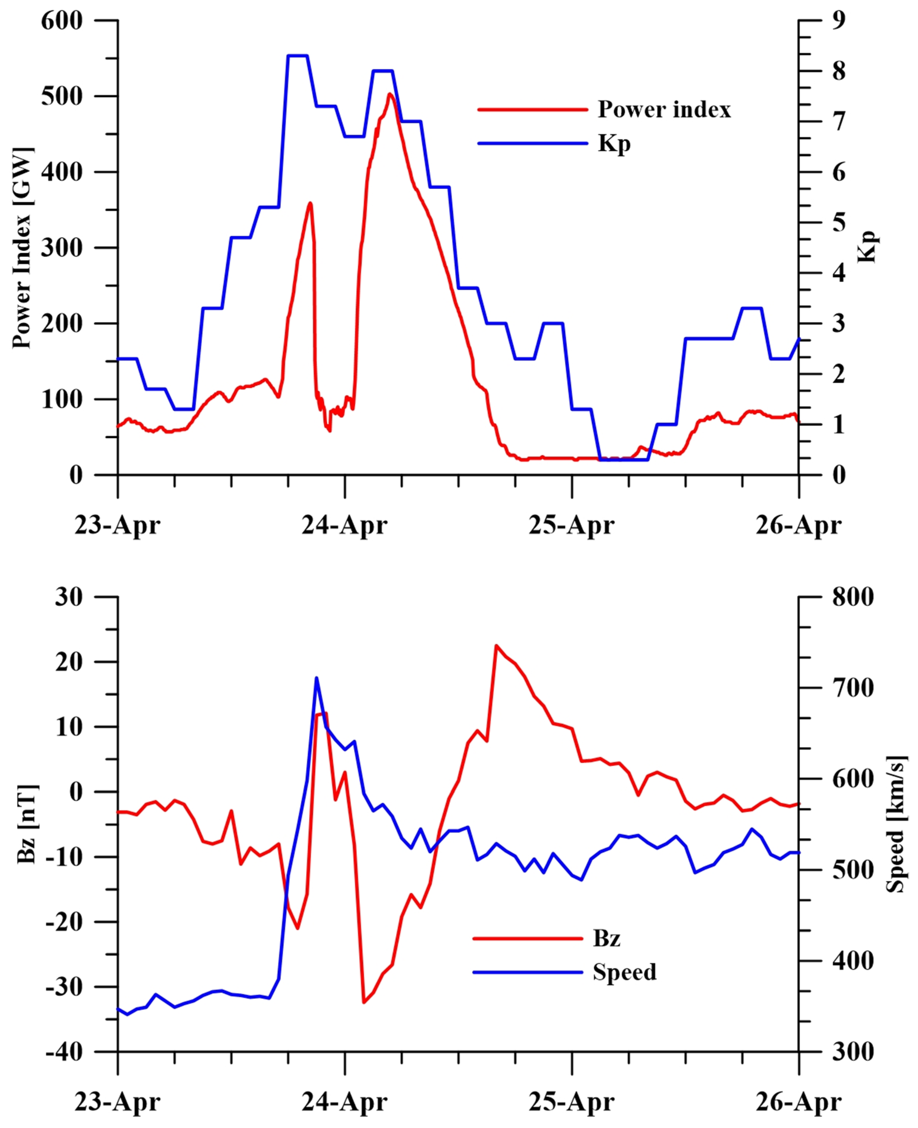
In order to trace the behavior of the geomagnetic disturbance, the indices describing the storm are presented in Figure 1. As seen in Figure 1 (top panel), the Kp-index gradually reaches values above 8 in the hours just before 18 UTC on 23 April 2023. According to the NOAA Space Weather Scales, the observed event is of Class G4 (Severe) [30]. According to the classification, a storm of Class G4 can cause some problems related to: (i) power systems—voltage control problems; (ii) spacecraft operations; and (iii) other systems: HF radio propagation, satellite navigation, low-frequency radio navigation. The time period in which Kp ≥ 5 is from 12 UTC on 23 April to 13 UTC on 24 April. The behavior of the geomagnetic indices and solar wind parameters (see Figure 1) shows that the storm has two sharply distinguished stages.
During the first stage of the considered event until 18 UTC on 23 April, the Bz component of the IMF is negative (southward) and has the opposite direction to the Earth’s magnetic field, leading to changes and the reconnection of IMF and the Earth’s magnetic field. The parameter indicating the speed of the solar wind clearly illustrates a sharp increase in its values from about 350 km/s (quiet conditions speed) to over 700 km/s in the hours before 20 UTC, which is another indication of the geomagnetic storm occurring. At around 21–22 UTC, there is about a four-hour period of positive Bz values in which the Power index decreases to a value close to that before the onset of the storm. The next phase of the storm begins around 01 UTC on 24 April and ends around 12 UTC on 24 April when the Bz component becomes positive again and the coupling of the Earth’s magnetosphere to the solar wind ceases.
To investigate the ionospheric response, the latitudinal and longitudinal distribution of the TEC response during the storm, represented by the values of the relative deviation from the running hourly medians, is considered.
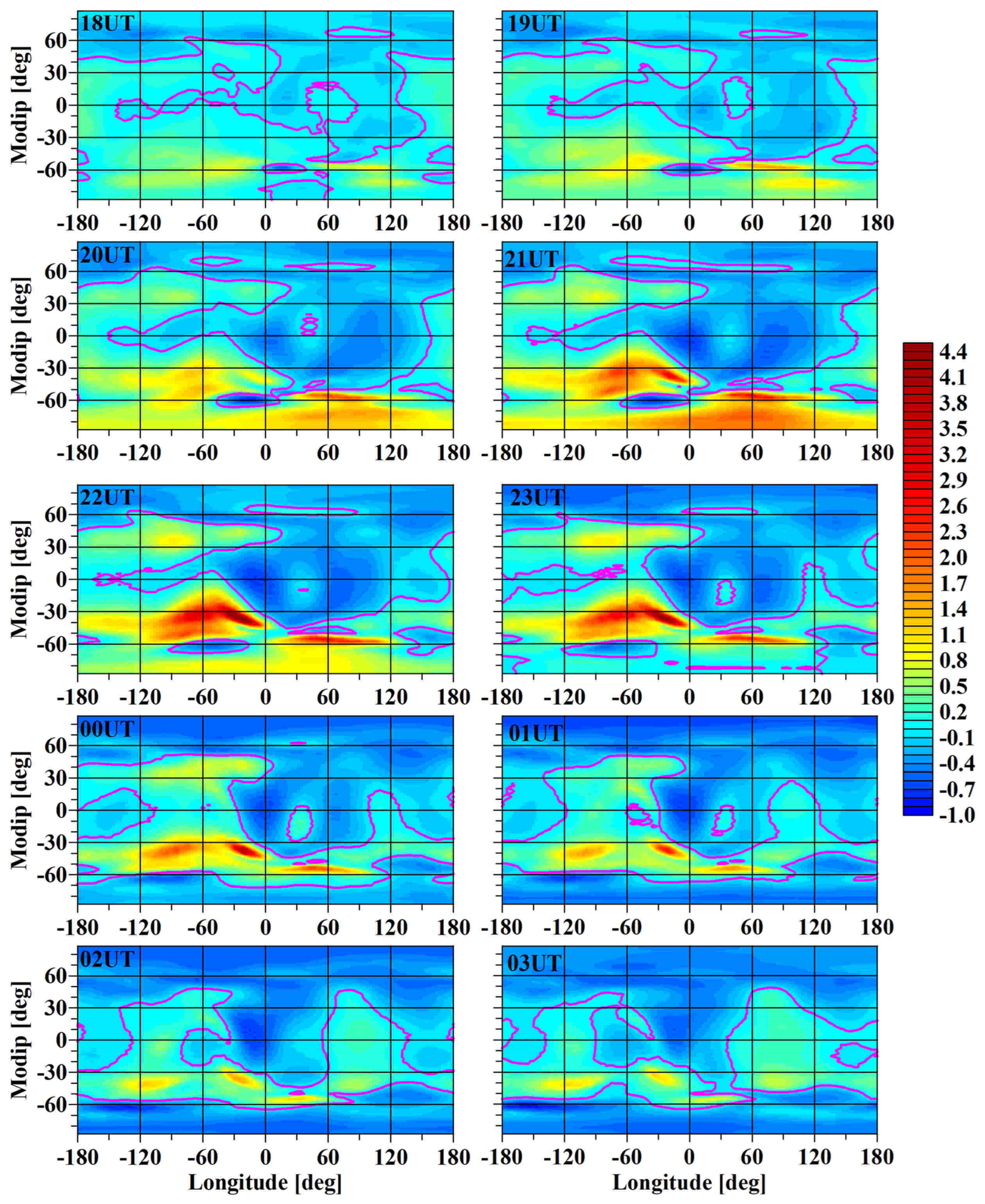
The results are shown in Figure 2 and Figure 3 in the form of spatial maps plotted in the longitude-modip. It can be seen from Figure 2 that on 23 April at 18 UTC, two characteristic regions of positive anomaly began to appear in the Southern Hemisphere. The two positive anomalies in TEC are located around 60° S, 60° E and 30° S, 60° W. These positive responses increased until around 00 UTC on the next day (24 April), after which they began to decrease.
An interesting fact about the region 60° S, 60° E is that it coincides with the night sector and the southern polar oval, which gives us reason to assume that this is the region of particle precipitation in the Southern Hemisphere. Symmetrical to the resulting Southern Hemisphere anomalies, a weak positive response was also observed in the Northern Hemisphere at 19–22 UTC on 23 April around 60° N, 90° E. In both cases, the probable reason for the positive response in TEC is direct ionization under the action of solar wind particles entering the auroral ovals. From the results shown in Figure 2 and Figure 3, it can be seen that the relative influence of additional ionization is stronger in the Southern Hemisphere where conditions approach winter conditions—i.e., observed a decreased electron density.
The second observed region of positive anomaly located around 30° S, 60° W has a complex structure where a split is observed around the 60° W meridian where the two parts move in opposite directions. In addition, an almost symmetric but weaker response is observed in the Northern Hemisphere at the latitude 30° N, especially distinct around 21–23 UTC on 23 April.
A similar positive ionospheric response was obtained in another paper [31]. In this study of the response of the equatorial ionosphere during geomagnetic storm on 15 July 2000 for the point FORT (Fortaleza, Brazil) with coordinates 3.85° W, 38.45° S, the authors explain the obtained positive response of vertical TEC with the theory of ionospheric disturbance dynamo. The use of point data from Jicamarca radar observations of F region vertical plasma drifts and indices of the auroral electrojet allowed them to determine the storm time dependence of the equatorial disturbance dynamo zonal electric fields [32].
An analogous result of an increase in the ionospheric electron density values was also obtained for the Halloween geomagnetic superstorm that occurred on October 29–30 2003 over the American longitude sector (~70° W). The results in this paper show that the observed TEC enhancement at higher latitudes is the result of the expansion of the equatorial ionization anomaly, while the obtained TEC enhancement at low- and mid-latitudes is the result of storm-generated equatorward neutral winds in addition to the eastward penetration electric field [33].
The papers described above in which analogous positive ionospheric responses were obtained provide possible explanations for the observed response in Figure 2 and Figure 3.
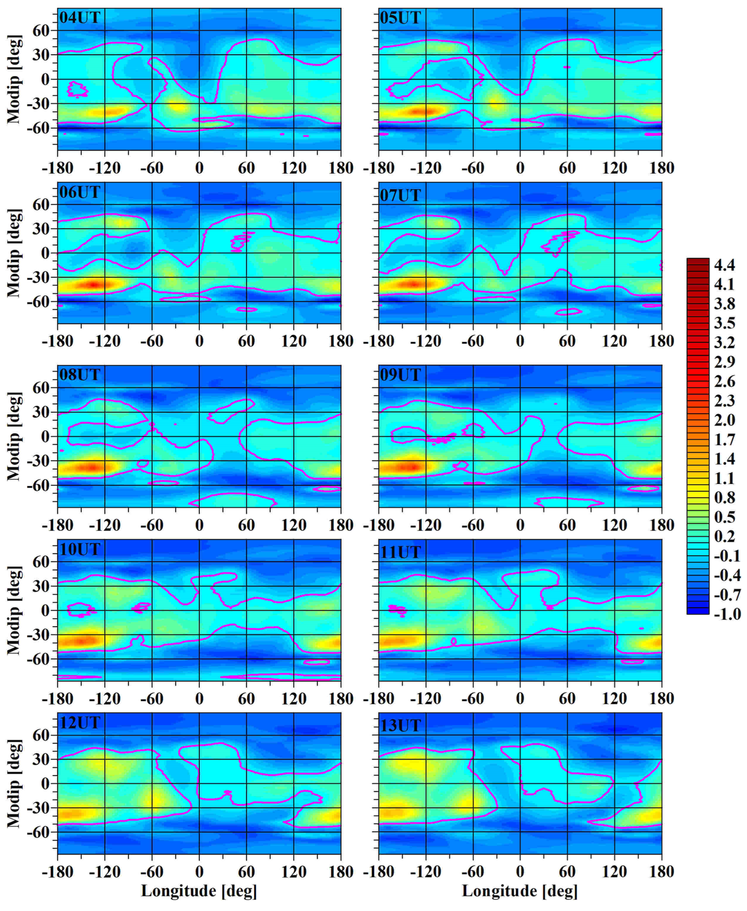
The secondary particle precipitation in the early morning hours (in UTC) coincides with the intensification of the positive response at 120° W in the Southern Hemisphere. Until the end of the geomagnetic storm, this positive response remained at the same longitude and latitude (see Figure 3, in the hours between 19 and 22 UTC).
For comparison of the obtained result of a negative response of TEC in the Northern Hemisphere, a study of the same geomagnetic storm, but based on single-point station measurements, is considered [34]. In this study, variations in the critical frequency foF2 were examined for the period from April 23 at 10 UTC to April 24 at 06 UTC from the ionograms, received at the Leibniz-Institutfür Atmosphären Physik (IAP) with ionosonde coordinates 52.21° N, 21.06° E (access available at: https://www.iap-kborn.de, accessed on 23 April 2023). The results of the foF2 behavior show a decrease in the critical frequencies from 8 MHz to 2 MHz (negative response) according to the IAP ionospheric station data. The results obtained for a specific IAP station coincide with the obtained negative anomaly for the Northern Hemisphere from the global TEC data presented in Figure 2 and Figure 3 [34].
Figure 4 shows in more detail the maps for 21 UTC on 23 April and 05 UTC on 24 April. The selected hours coincide with the two maxima of the Power Index, i.e., of the energy entering the auroral regions. Figure 4 (top panel) shows that the positive response at 60° S occurs at 1 h in local time, i.e., close to midnight. The positive response at about 30° S occurs at local time between 17 and 19, which can be considered the approximate time of sunset in winter conditions. The presented map at 05 UTC on 24 April (see Figure 4, bottom panel) shows a weak positive response at 60° S at the zero meridian and corresponding local time at 5. The most significant positive response shown in Figure 4 (bottom panel) is located at 30° S and 120° W. The analogous positive response in the Northern Hemisphere is around 40° N and 120° W.
From the results presented in Figure 4, it can be seen that the behavior of the relative TEC in the two auroral regions gives us reason to assume the location of the areas of strongest thermal impact of the particle precipitation in the both hemispheres. The first particle precipitation probably causes heating of the region around 60° E where the strongest positive TEC response occurs (Figure 4, top panel). The second particle precipitation is weaker and is manifested by additional ionization, although it is energetically stronger and can be assumed to be localized around the zero meridian (see Figure 4, bottom panel). A possible reason for its weak manifestation in TEC is the fact that the area of particle precipitation was already significantly heated by the previous precipitation, in which the change in the O/N2 ratio caused an increase in recombination and correspondingly a decrease in the effect of additional ionization. Evidence for this assumption is the presence of an area of extreme negative response in the Northern Hemisphere (see Figure 4, bottom panel).
Additional investigation of the positive anomaly observed in the Western Hemisphere is presented in Figure 5. The plot illustrates the variations in the relative critical frequency foF2, whose data are received from the ground-based ionospheric station for vertical sounding Cachoeira Paulista (23.2° S modip, 50° W) marked in a blue color. The same figure also shows the behavior of the relative TEC at the closest point by coordinates to those of the selected station (22.5° S modip, 50° W) from the map of the TEC data (marked in red in Figure 5). The positive responses of both quantities with a maximum around 22 UTC on 23 April show a complete coincidence (see Figure 2).The latitudinal location of the positive anomaly in the Western Hemisphere, which has symmetry with respect to the magnetic equator, suggests that this anomaly is due to a forced fountain effect. A possible explanation for the observed positive response during the night hours (unlike quiet conditions) may be due to the reverse fountain. One possible hypothesis for the action of this important mechanism is related to the increase in ionization at equatorial anomaly latitudes in the night hours, with some contribution from the prereversal strengthening of the forward fountain [35]. An additional argument for the stated hypothesis is the appearance of a region around the magnetic equator where the TEC response is negative. It should be expected that the plasma transfer from the equator to the mid-latitudes will be accompanied by the reduction in plasma around the equator. Assuming that the observed anomaly in the latitudinal range between 30° S and 30° N is due to DDEF (Disturbed Dynamo Electric Fields) for the selected ionospheric storm, a number of peculiarities are noted.
In order to obtain a more detailed view of the place where the maximum response was obtained in relative TEC for the period 23–25 April, spatial maps of the amplitudes and phases of SPW1 are presented. The amplitude map (see Figure 6a) presents the two activations of the response at latitudes 30° S and 30° N coincident in time with the two particle precipitations according to the solar and geomagnetic parameters illustrated in Figure 1. From Figure 6b, it can be seen that the SPW1 phases (i.e., the location of the positive maxima) at these two latitudes during the storm occur in the Western Hemisphere.
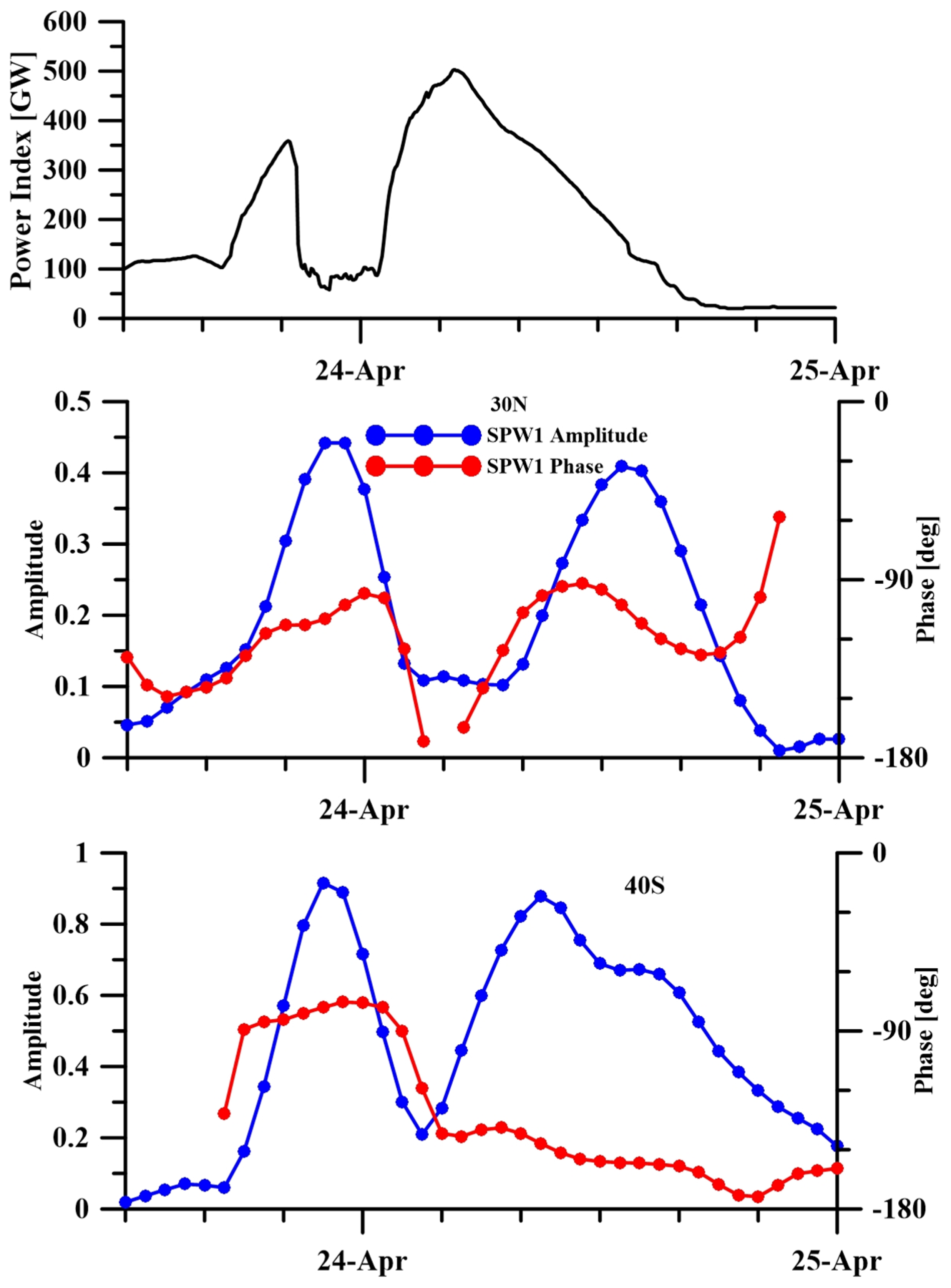
Figure 7 presents a comparison of the behavior of the amplitude and phase of SPW1 for the locations in the two hemispheres, where a positive response occurs in the ionospheric TEC. The upper panel shows the Power Index, which indicates the moment of increase in incoming solar radiation coinciding in time with the onset of the geomagnetic storm according to the considered parameters in Figure 1.
The asymmetry of the response in the two hemispheres, northern and southern, can be explained by two hypotheses.
Due to the fact that the conditions in the Southern Hemisphere are close to winter, it should be expected that the temperature of the neutral air is lower than that in the Northern Hemisphere; therefore, particle precipitation can cause a stronger warming, therefore a relatively more significant disturbed wind in the Southern Hemisphere. It should be emphasized that the relative TEC deviation used is relative to quiet ionospheric conditions, which condition also includes the condition of the neutral atmosphere during the given month of the year. Additionally, in the present work, selected ionospheric storms that occurred in the months of June and December (summer and winter solstice), which show the same dependence on the season, are considered.
The second essential peculiarity of the ionospheric response is the longitudinal distribution of the response. The maximum positive response is observed only in the Western Hemisphere, although particle precipitation continues (with a short interruption) throughout the day. An illustration of this feature is the behavior of the amplitudes and phases of the approximation of the longitudinal distribution of the relative TEC by SPW1, which is an approximation of this distribution by the cosine with a spatial period of 360 geographic degrees shown in Figure 6. The maps illustrated in Figure 2, Figure 3 and Figure 4 show that this representation reflects the main peculiarities of the longitudinal distribution of the relative TEC response. As mentioned in Section 3.2. Methods and methodologies, and more specifically in the “Method of stationary amplitudes and phases”, the amplitude reflects the maximum deviation from the zonal mean value of the relative TEC, and the SPW phase indicates the latitude of the positive maximum of the response at a given hour. To follow in detail the positive anomaly in TEC for the considered storm in April 2023, Figure 7 shows the amplitudes and phases of SPW1 at the latitudes 30° N and 30° S. The results show that the phases show an apparent stationarity. In the Northern Hemisphere during the activation of SPW1, they appear in the limits around 90° W–120° W, and in the Southern Hemisphere around 90° W–150° W, respectively. This result coincides with the spatial distribution of relative TEC shown in Figure 2 and Figure 3.
3.2. Geomagnetic Storm 22–24 June 2015
The purpose of studying this event is the opportunity to investigate the storm effects in ‘opposite’ seasons—summer and winter.
According to the behavior of the geomagnetic indices Dst and Kp, shown in Figure 8 upper panel, 18 UTC on 22 June 2015 is determined as the beginning of the geomagnetic storm. This storm is occurring in several stages. In the first stage, the Kp-index reaches almost 9 while the Dst-index has a value of about −120 nT in the hours around 19 UTC. According to the classification of the Kp-index, this storm is similar to the above mentioned event in April 2023 both in terms of the value of the index and in its biphasic manifestation (with two expressed maxima in the Kp-index). According to the classification, the investigated storm is of the Strong class because it corresponds to the cases when −100 > Dst > −200 nT [36,37]. The second stage, which is clearly visible from the indices in Figure 8 upper panel, has a maximum manifestation at around 04 UTC on 23 June 2015. According to the value of the Kp-index, which in this case is almost 8, the considered geomagnetic storm is of the Strong type. The difference compared to the first geomagnetic event is that in the first case the Kp-index reacts more strongly, while in the second case according to the Dst-index (which has values around −210 nT) the storm is of the Severe class. As seen in Figure 8 bottom panel, three consecutive periods of negative Bz values (i.e., interaction of the solar wind and the Earth’s magnetosphere) are observed during the geomagnetic storm. The first period occurs around 18 UTC on 22 June 2015 and coincides with the sudden increase in solar wind speed. The second moment of the negative Bz component of the IMF is around 02 UTC on 23 June 2015, and the third (which is the weakest) is around 08 UTC on 23 June 2015. The active phase of the storm can be considered to end around 12 UTC on 23 June, when the Bz component of the IMF has a stable positive value and the Kp-index has values below 3.
In order to make an analogous study of the maximum manifestation of the TEC response in Figure 9, the amplitude and phase maps of SPW1 are presented. The maps show a strongly increased modip amplitude at the 60° S latitude with similar time but weaker activation at the 45° N latitude. Similarly, in this storm, a strong response is observed in the winter hemisphere. The SPW1 activation on 23 June 2015 has maxima at 40° S and at the equator, with a larger amplitude in the Southern Hemisphere, confirming the well-known seasonal response in winter conditions [28,29].
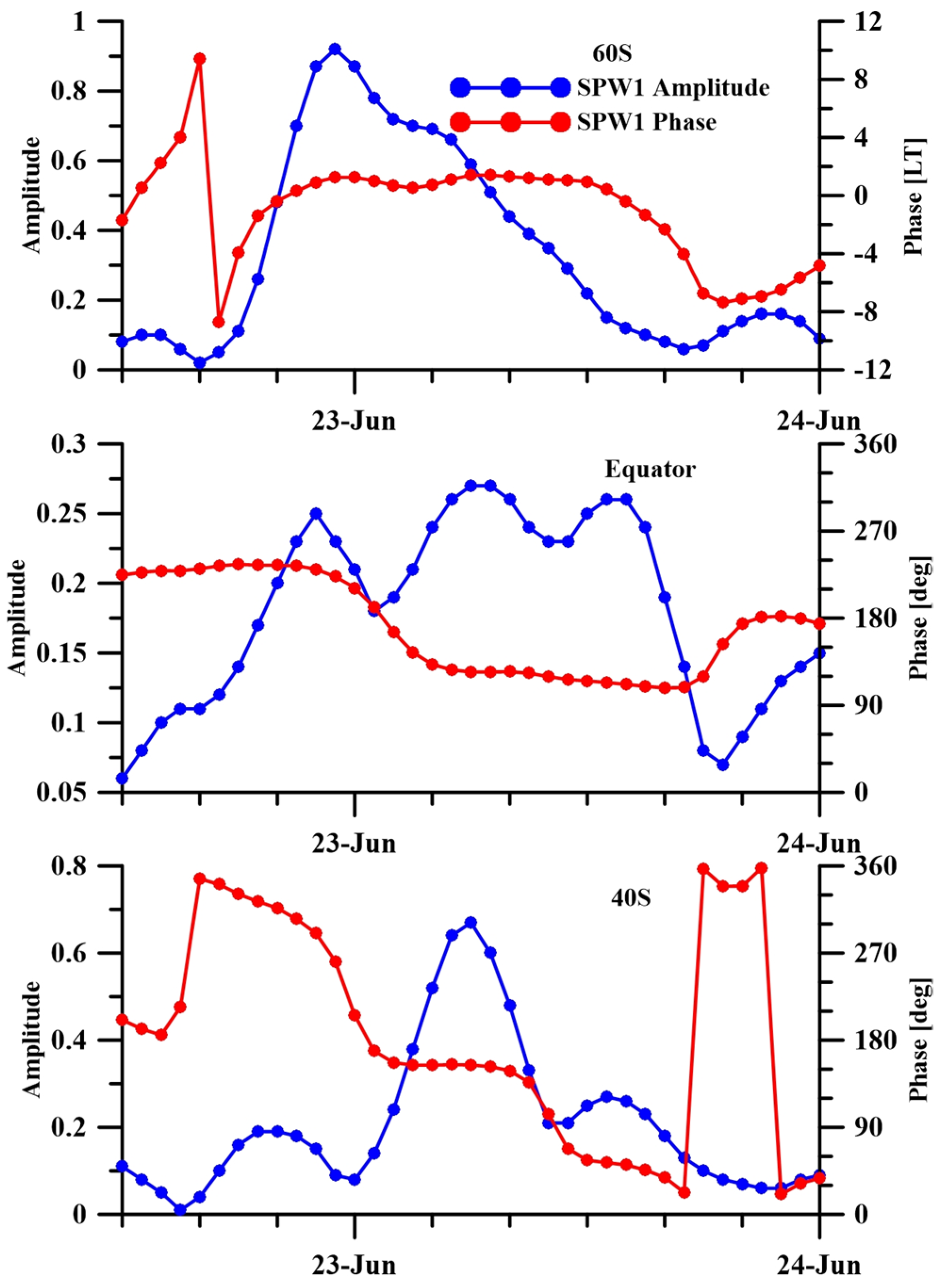
Figure 10 shows the amplitude and phase variability of SPW1 at three characteristic latitudes. At the latitude 60° S, the amplitude is maximal around 23 UTC on 22 June 2015, when the first particle precipitation is caused by the negative values of the Bz component. The phase in LT until the end of the storm is close to zero, which means that the impact on the ionosphere is shifted along with the local midnight region, which means that the positive maximum of the ionospheric response is related to the ionization of the particle precipitation region. The positive maxima of the response in the equatorial region and in southern midlatitudes, however, have quite different behavior. The phase, i.e., the positive maximum, is almost stationary and is located in the Western Hemisphere at the beginning of the geomagnetic storm. At both latitudes, the phase tends to decrease, i.e., westward direction change, but this variation is too slow compared to the movement of the midnight meridian over time. As in the previous storm considered, the low and mid-latitude anomaly has two maxima, suggesting that it is caused by a “fountain effect”. Compared to the April 2023 storm, there is a tendency for the response to shift to southern latitudes (i.e., in the winter hemisphere).
The considered event is well studied and described in a significant number of papers, and the results of the type of ionospheric response are analogous to the presented amplitudes and phases of SPW1 illustrated in Figure 9 and Figure 10.
In the first paper about the geomagnetic storm on 22–23 June 2015, the authors use different types of ground-based instruments and data of multiple satellite missions to study equatorial and low-latitude electrodynamic and ionospheric disturbances. Several conclusions are drawn from the results in this investigation. PPEF have considerable impact on the equatorial electrojet and the equatorial zonal electric at the beginning of the storm. The significant ionospheric uplift and positive ionospheric storm on the day side, and downward drift on the night side observed by the authors, they explain, is due to the eastward direction of the PPEF. Some variations in the equatorial electrojet at the end of the main phase were also obtained, which the authors conclude are the result of the disturbance dynamo effect was already in effect, competing with the PPEF and reducing them. The authors of this paper associate the observed second positive storm with the influence of a disturbed thermosphere [38].
The second global study of the response of the ionospheric TEC during the geomagnetic storm on 22 June 2015 shows the following results: (a) before the main phase of the considered geomagnetic storm, increases in TEC at high latitudes were obtained; (b) there was a difference in the TEC response at mid and low latitudes in the Northern Hemisphere and the Southern Hemisphere and decreases at equatorial latitudes. The author explains the observed ionospheric response of the equatorial and low latitudes during the main phase of the storm with the influence of these areas by Prompt Penetration Electric Fields [39].
Another investigation of the ionospheric effect of the same event in June 2015 for the South American region is based on a comparison between different measurements. Based on the large number of different types of data used, the authors illustrate and explain the observed expansion of the crest of EIA (Equatorial Ionization Anomaly) at mid-latitudes and high latitudes mainly due to PPEF during the main phase and the recovery phase of the geomagnetic storm during the day [40].
3.3. Geomagnetic Storm 14–16 December 2006
The selected geomagnetic storm is close to the winter solstice in the Northern Hemisphere. In order to examine in detail the behavior of the geomagnetic storm, Figure 11 shows the geomagnetic indices Kp and Dst (top panel) and the solar parameters of the Bz component of IMF and the solar wind speed (bottom panel).
The behavior of the Kp-index shows a sudden increase after 12 UTC on 14 December, 2006, when the quantity has values above 5. At around 00 UTC on 15 December, maximum Kp values of almost 9 were also recorded. According to the classification of this index, the event under consideration is of Class G4 (Severe), analogous to the events discussed above. The recovery of index values to quiet conditions was observed a few hours before 00 UTC on 16 December. According to the behavior of the Kp- and Dst-indexes, the considered geomagnetic storm had a sudden onset, occurring around 23 UTC on 14 December 2006. In this particular case, the Dst values reach about −160 nT over a period of about 7–8 h, which is also the time of the main phase of the storm. The recovery phase of Dst continues until 17 December 2006.
An analogous representation of the behavior of the solar wind parameters shows a sharp increase in the solar wind speed to about 950 km/s around 14 UTC on 14 December 2006. After that, the speed gradually decreases (see Figure 11 bottom panel).
Special attention should be paid to the behavior of the Bz component of the IMF for the considered time interval (see Figure 11 bottom panel). The moment of increase in the speed of the solar wind coincides in time with the short-term interaction of the Earth’s magnetosphere and the solar wind, described by the small negative values of Bz (which indicates the moment of interaction between the solar wind and the Earth’s magnetosphere). The considered parameter has positive values between 18 UTC on 14 December and in the hours between 20–21 UTC on 14 December, when the Bz component reaches negative values. The minimum of the Bz component of the IMF is at 00 UTC on 15 December 2006, coinciding in time with the most significant responses and in the geomagnetic indices presented in Figure 11 top panel.
Again, an investigation of the ionospheric response is suggested by the resulting SPW1 amplitude and phase maps shown in Figure 12. It can be seen from the figure that the maps presented in Figure 12 show a visible similarity to those illustrating the geomagnetic storm in June 2015 (see Figure 9), with the amplitudes of the ionospheric response again being higher in the winter hemisphere (in this case for geomagnetic storm on 15 December 2006—this is the Northern Hemisphere).
Between 18 UTC and 24 UTC on 14 December, an activation of SPW1 amplitude was observed at modip latitudes of 60° N and 60° S (modip latitudes close to the northern and southern auroral ovals). At lower latitudes, the response maximizes on 15 December around 06 UTC, being stronger in the Northern Hemisphere.
The investigated geomagnetic storm in December 2006 is of interest to scientists and has been studied by a large number of authors [41,42,43]. In the first discussed paper in which the response of the ionosphere was studied, a considerable positive response was obtained over the Atlantic sector after the onset of considered storm. The authors explain the observed positive anomaly during the initial phase with changes in the electric fields, also mentioning a possible influence as a result of neutral winds and composition changes. An observed result in this study is that the reduction in electron densities in the two hemispheres is different, being much more rapid in the winter hemisphere. The authors explain the differences in the positive ionospheric response for the two hemispheres with the presence of electric fields and their influence on the electron density [41].
The second work, the result of which confirms the results seen in the present investigation for the geomagnetic storm on 15 December 2006, is based on a combination of different types of measurements, allowing the study of the ionospheric positive response by revealing the storm time response in different altitude regions [42]. The results of this study show an analogous response to that in [41], characterized by electron density enhancements at low latitudes to mid-latitudes during the main phase of the storm. The positive anomalies, analogous to those obtained in the present study, which the authors obtain for the Pacific Ocean region remain present in the equatorial ionization anomaly crest regions at the hours 12:00 UTC on 15 December. The authors explain the observed positive responses with the enhanced eastward electric field and equatorward neutral wind [42].
The third case, which is used for comparison, is a study of observations related to the generation of equatorial ionospheric anomalies including ionospheric plasma bubbles and variations in the ionospheric F-region in the South American sector during the same geomagnetic storm in December 2006. The authors investigated the anomalies in the F-region based on two ionospheric stations during the night hours of 14–15 December, namely São José dos Campos (SJC, 23.2° S, 45.9° W; dip latitude 17.6° S), and Port Stanley (PST, 51.6° S, 57.9° W; geom. latitude 41.6° S), which show strong oscillations due to the propagation of traveling ionospheric disturbances by the Joule heating in the auroral region. Unlike the F-region response, the anomaly for VTEC obtained by the authors is both positive and negative, and the explanation of the observed response for the South American sector proposed by the authors is related to changes in the O/N2 ratio in the Southern Hemisphere [43].
Shown in Figure 13, the behavior of the amplitudes and phases at three characteristic latitudes is very similar to the analogs of the two storms discussed above (see Figure 7 and Figure 10). It can be seen from the figure that the response phase at 65° N expressed in local time is close to 0 LT. At latitudes of 30° S and 30° N, the phase is again stationed in the Western Hemisphere, in this case near the longitude 180°.
4. Discussion
Due to the characteristic features of the longitudinal distribution of the ionospheric response, an analysis method was used based on the approximation of the longitudinal distribution of the relative deviation of the TEC from the medians with a cosine with a spatial period of one full angle (360°) for each specific hour of the storms, which representation is analogous to a quasi-stationary wave with wavenumber 1. Based on the data from the global distribution of TEC for the geomagnetic storm on 24 April 2023, arguments are presented that the proposed representation by the course of the amplitudes and phases of this quasi-stationary wave, allowing us to illustrate the main features of the positive responses of TEC and their behavior in latitude, longitude and over time. The TEC data are interpolated into the coordinate system of modified dip latitude, geodetic longitude.
Positive anomalies in the region of the auroral oval are registered in all three storms in the night sector, in most cases near midnight local time (see Figure 4, Figure 10 and Figure 12).
An interesting result was obtained for the geomagnetic storm on 22–24 June, for the SPW1 amplitudes and phases at 60° S illustrated in Figure 10 (top panel). The considered storm has long-lasting particle precipitation in the auroral oval. It can be seen from the figure that the retention of the phase (expressed in local time) close to zero is almost one day. This indicates that the impact on the ionosphere follows the displacement of the midnight meridian. This gives us reason to consider that the increase in electron density (respectively, TEC) in the auroral region is due to additional ionization from particles precipitation of the solar wind entering the atmosphere. The effect is strong in the winter hemisphere due to the low electron density in winter during nighttime conditions [2,28,29,41,44].
There is reason to assume that exactly in this region the intense heating of the neutral air takes place, which also causes the ionospheric response outside the auroral region.
Figure 14 shows the phase behavior of the positive response for the three storms at selected latitudes where the response is most significant. One day is shown for each storm. In all three storms, the storm maximum in the Kp-index is around midnight on UTC, and the observed maximum positive response is during the next 24 h, which is shown in Figure 14.
For all three storms at 00 UTC and a few hours after, the maximum response occurs in the Earth’s daytime region, between local noon (−12 LT) and around local sunset. But during the day, this maximum turns out to be in the night part. The increase in the phase in local time means a westward shift of the maximum, which can also be seen in Figure 7, Figure 10 and Figure 13, but the shift velocity is smaller than the Earth’s phase rotation velocity. The maps illustrated in Figure 6, Figure 9 and Figure 12 show that this phenomenon covers a considerable latitudinal zone, including low and partly mid-latitude modip latitudes, not just the particular latitudes of maximum occurrence.
It is well known that a fully stationary SPW1 should have a phase variation in local time of 24 h per day, and a rotating one with the rotation of the midnight point should have a constant phase in local time.
The results show that the two studied geomagnetic storms in December 2006 and April 2023 have a slower westerly displacement than the June 2015 geomagnetic storm. It is possible that this result is due to seasonal differences, but based on the available material it cannot be established with certainty and therefore future analysis is envisaged.
The observed peculiarities in the response of TEC at low and mid-latitudes allow to make a hypothesis about their occurrence, a hypothesis which is maximally simplified. In accordance with the classical theory of a disturbed dynamo, the reason for the appearance of a positive anomaly at low latitudes is a vertical drift of the ionospheric plasma caused by electric currents under the action of the equatorward flow in both hemispheres [1]. This flow is induced by the heating of the polar oval in the midnight region.
Under the action of the Coriolis acceleration when entering low latitudes, the direction changes from meridional to zonal, which creates currents in the dynamo region and due to the interaction with the Earth’s magnetic field, a vertical drift of the ionospheric plasma occurs and the creation of the so-called “fountain effect”. The considered positive responses of the low-latitude ionosphere have a number of peculiarities that correspond to this mechanism. In the analysis of the specific ionospheric storms, a distinct split of the positive response is observed, which gives us reason to assume the presence of a “fountain effect” [35].
Another result that is observed is a shift of the response in latitude and intensity to the winter hemisphere, which can be explained by the low temperature of the atmosphere in the winter polar regions and, accordingly, the larger temperature difference compared to the quiet conditions under the influence of particle precipitation from the solar wind.
A significant deviation from the theory is the stationing of the low-latitude positive anomaly observed during the storms, in which the location of the observed response and the longitudinal distribution shifts too slowly in the east–west direction. In all three considered storms, the location of the positive anomaly is located in the auroral region and clearly follows the movement of the midnight region from west to east with a velocity matching the velocity of the Earth’s rotation.
In the present work, the following hypothesis is proposed for the cause of this phenomenon.
In the examined storms, the positive response of TEC is observed in the auroral region, which, as a rule, has a short-term variability and coincides with the time of the initial particle precipitation. For example, during the storm in April 2023, the repeated particle precipitation did not cause a significant positive response in the auroral region, unlike the first particle precipitation, which had even lower energy indicators (see Figure 1).
There is reason to assume that additional heating also has a peculiarity analogous to additional ionization. If this hypothesis is accepted, it turns out that the intense heating of the neutral air is concentrated in a relatively limited region. As a result, the equatorward flow created by it has a relatively stable longitudinal structure associated with the area of auroral heating decreases as a result of the cooling of the heated region, a process which is inert.
The proposed hypothesis does not exclude the expansion of the heated auroral region in the western direction under the influence of the displacement of the midnight meridian. As a result, the observed displacement of the positive low-latitude anomaly can also be caused in the western direction, but at a significantly lower velocity due to the inertia of the heating and especially of the cooling of the neutral air in the auroral latitudes.
However, the proposed hypothesis can hardly fully explain the manifestation of the low-latitude positive anomaly west of the midnight meridian, where the auroral response is observed (see Figure 2, Figure 3 and Figure 4). Detailed maps of the April 2023 storm presented show that the longitudinal distribution of the low-latitude response is complex. The system of disturbed dynamo currents is more complex than it was represented by the simplified cosine approximation used in the present work.
5. Conclusions
Three geomagnetic storms that occurred on (i) 23–24 April 2023, (ii) 22–24 June 2015 and (iii) 14–16 December 2006 are analyzed in the present investigation. All three disturbances considered are of the same intensity G4 according to the NOAA Space Weather Scales. All three storms have practically the same duration of about one day and all three reach their maximum manifestation at around 00 UTC. The first storm occurs between the winter and summer solstice in the Northern Hemisphere. The second coincides with the summer solstice, and the third is close to the winter solstice. The main attention in the analysis of the present study is paid to the positive responses in the ionospheric TEC at latitudes close to the auroral ovals and at mid- and low latitudes.
The positive responses in mid- and low latitudes in the three considered storms have the following peculiarities:
- The positive responses have two maxima, which are either practically symmetrical to the magnetic equator (the geomagnetic storms in April 2023 and December 2006) or are shifted in the direction of the winter hemisphere (the geomagnetic storm in June 2015);
- The response in the winter hemisphere is more significant and strong. It was found that the responses at these latitudes noticeably lag compared to those over the auroral regions;
- An important feature observed in all three storms is the location of the maximum of the positive response;
- The three investigated geomagnetic storms show a common regularity. The longitudinal distribution of the response in low latitudes appears to be relatively stationary with respect to geographic coordinates, with a westward displacement observed with a phase velocity smaller than the Earth’s rotation velocity. This indicates that the low-latitude response is not directly related to local weather.
Author Contributions
Conceptualization, R.B. and P.M.; methodology, P.M.; software, P.M.; validation, P.M. and R.B.; formal analysis, P.M.; investigation, R.B.; resources, R.B.; data curation, P.M.; writing—original draft preparation, R.B.; writing—review and editing, R.B.; visualization, P.M.; supervision, R.B.; funding acquisition, R.B. All authors have read and agreed to the published version of the manuscript.
Funding
This work was supported by Contract No. DO1-404/18.12.2020—Project “National Geoinformation Center (NGIC)” financed by the National Roadmap for Scientific Infrastructure 2017–2023. This work was partially supported by the Bulgarian Ministry of Education and Science under the National Research Program “Young scientists and postdoctoral students-2”, approved by DCM № 206/07.04.2022.
Institutional Review Board Statement
Not applicable.
Informed Consent Statement
Not applicable.
Data Availability Statement
The global maps of TEC data are available for free at https://www.izmiran.ru/ionosphere/weather/grif/Maps/TEC/, accessed on 19 February 2024. Data from individual points, measured by ionosondes, are provided by the Global Ionosphere Radio Observatory (GIRO) at this link: https://giro.uml.edu/didbase/scaled.php, accessed on 19 February 2024. The indices of geomagnetic activity, namely Dst-index and Kp-index and Bz component of IMF are received from https://omniweb.gsfc.nasa.gov/, accessed on 19 February 2024. The Power Index is available at http://services.swpc.noaa.gov/text/aurora-nowcast-hemi-power.txt, accessed on 19 February 2024. The data about solar wind speed is obtained from National Oceanic and Atmospheric Administration (NOAA)—Space Weather Prediction Center (https://www.cpc.ncep.noaa.gov/products/monitoring_and_data/oadata.shtml, accessed on 19 February 2024).
Acknowledgments
The authors express thanks to Goddard Space Flight Center for the freely available data of the Bz component, Dst-index and Kp-index. Special thanks to the Global Ionosphere Radio Observatory for ionospheric data from vertical sounding and global TEC data, which are freely available at website of the Institute of Terrestrial Magnetism, Ionosphere and Radio Wave Propagation (IZMIRAN). We are grateful to the NOAA, Space Weather Prediction Center, for the Power Index data provided.
Conflicts of Interest
The authors declare no conflicts of interest.
References
- Richmond, A.D.; Lu, G. Upper-atmospheric effects of magnetic storms: A brief tutorial. J. Atmos. Sol. Terr. Phys. 2000, 62, 1115–1127. [Google Scholar] [CrossRef]
- Danilov, A.D. Ionospheric F-region response to geomagnetic disturbances. Adv. Space Res. 2013, 52, 343–366. [Google Scholar] [CrossRef]
- Nishida, A. The origin of fluctuation in the equatorial electrojet; a new type of geomagnetic variations. Ann. Geophys. 1966, 22, 478–484. [Google Scholar]
- Jaggi, R.K.; Wolf, R.A. Self-consistent calculation of the motion of a sheet of ions in the magnetosphere. J. Geophys. Res. 1973, 78, 2852–2866. [Google Scholar] [CrossRef]
- Spiro, R.W.; Wolf, R.A.; Fejer, B.G. Penetrating of high-latitude-electric-field effects to low latitudes during SUNDIAL 1984. Ann. Geophys. 1988, 6, 39–49. [Google Scholar]
- Lu, G.; Goncharenko, L.; Nicolls, M.J.; Maute, A.; Coster, A.; Paxton, L.J. Ionospheric and thermospheric variations associated with prompt penetration electric fields. J. Geophys. Res. Space Phys. 2012, 117, 1–14. [Google Scholar] [CrossRef]
- Basu, S.; Basu, S.; Valladares, C.E.; Yeh, H.C.; Su, S.Y.; MacKenzie, E.; Sultan, P.J.; Aarons, J.; Rich, F.J.; Doherty, P.; et al. Ionospheric effects of major magnetic storms during the International Space Weather Period of September and October 1999: GPS observations, VHF/UHF scintillations, and in situ density structures at middle and equatorial latitudes. J. Geophys. Res. Space Phys. 2001, 106, 30389–30413. [Google Scholar] [CrossRef]
- Tsurutani, B.T.; Verkhoglyadova, O.P.; Mannucci, A.J.; Saito, A.; Araki, T.; Yumoto, K.; Tsuda, T.; Abdu, M.A.; Sobral, J.H.A.; Gonzalez, W.D.; et al. Prompt penetration electric fields (PPEFs) and their ionospheric effects during the great magnetic storm of 30–31 October 2003. J. Geophys. Res. Space Phys. 2008, 113, 1–10. [Google Scholar] [CrossRef]
- Abdu, M.A.; De Souza, J.R.; Sobral, J.H.A.; Batista, I.S. Magnetic storm associated disturbance dynamo effects in the low and equatorial latitude ionosphere. Recurr. Magn. Storms Corotating Sol. Wind. Streams 2006, 167, 283–304. [Google Scholar]
- Blanc, M.; Richmond, A.D. The ionospheric disturbance dynamo. J. Geophys. Res. Space Phys. 1980, 85, 1669–1686. [Google Scholar] [CrossRef]
- Richmond, A.D.; Roble, R.G. Electrodynamic coupling effects in the thermosphere/ionosphere system. Adv. Space Res. 1997, 20, 1115–1124. [Google Scholar] [CrossRef]
- Huang, C.M. Disturbance dynamo electric fields in response to geomagnetic storms occurring at different universal times. J. Geophys. Res. Space Phys. 2013, 118, 496–501. [Google Scholar] [CrossRef]
- Huang, C.S.; Wilson, G.R.; Hairston, M.R.; Zhang, Y.; Wang, W.; Liu, J. Equatorial ionospheric plasma drifts and O+ concentration enhancements associated with disturbance dynamo during the 2015 St. Patrick’s Day magnetic storm. J. Geophys. Res. Space Phys. 2016, 121, 7961–7973. [Google Scholar] [CrossRef]
- Balan, N.; Liu, L.; Le, H. A brief review of equatorial ionization anomaly and ionospheric irregularities. Earth Planet. Phys. 2018, 2, 257–275. [Google Scholar] [CrossRef]
- Abdu, M.A.; Sobral, J.H.A.; De Paula, E.R.; Batista, I.S. Magnetospheric disturbance effects on the equatorial ionization anomaly (EIA): An overview. J. Atmos. Sol. Terr. Phys. 1991, 53, 757–771. [Google Scholar] [CrossRef]
- Balan, N.; Shiokawa, K.; Otsuka, Y.; Watanabe, S.; Bailey, G.J. Super plasma fountain and equatorial ionization anomaly during penetration electric field. J. Geophys. Res. Space Phys. 2009, 114, 1–10. [Google Scholar] [CrossRef]
- Danilov, A.D.; Lastovicka, J. Effects of geomagnetic storms on the ionosphere and atmosphere. Int. J. Geomagn. Aeron. 2001, 2, 209–224. [Google Scholar]
- López-Urias, C.; Vazquez-Becerra, G.E.; Nayak, K.; López-Montes, R. Analysis of Ionospheric Disturbances during X-Class Solar Flares (2021–2022) Using GNSS Data and Wavelet Analysis. Remote Sens. 2023, 15, 4626. [Google Scholar] [CrossRef]
- Pazos, M.; Mendoza, B.; Sierra, P.; Andrade, E.; Rodríguez, D.; Mendoza, V.; Garduño, R. Analysis of the effects of geomagnetic storms in the Schumann Resonance station data in Mexico. J. Atmos. Sol. Terr. Phys. 2019, 193, 105091. [Google Scholar] [CrossRef]
- Wang, W.; Lei, J.; Burns, A.G.; Solomon, S.C.; Wiltberger, M.; Xu, J.; Zhang, Y.; Paxton, L.; Coster, A. Ionospheric response to the initial phase of geomagnetic storms: Common features. J. Geophys. Res. Space Phys. 2010, 115, 1–18. [Google Scholar] [CrossRef]
- Rawer, K. Encyclopedia of Physics. In Geophysics III, 1st ed.; Rawer, K., Ed.; Springer: Berlin/Heidelberg, Germany, 1984; Part VII; pp. 389–391. [Google Scholar]
- Rawer, K.; Kouris, S.S.; Fotiadis, D.N. Variability of F2 parameters depending on modip. Adv. Space Res. 2003, 31, 537–541. [Google Scholar] [CrossRef]
- Azpilicueta, F.; Brunini, C.; Radicella, S.M. Global ionospheric maps from GPS observations using modip latitude. Adv. Space Res. 2006, 38, 2324–2331. [Google Scholar] [CrossRef]
- Mukhtarov, P.; Pancheva, D.; Andonov, B.; Pashova, L. Global TEC maps based on GNSS data: 1. Empirical background TEC model. J. Geophys. Res. Space Phys. 2013, 118, 4594–4608. [Google Scholar] [CrossRef]
- Fu, W.; Ma, G.; Lu, W.; Maruyama, T.; Li, J.; Wan, Q.; Fan, J.; Wang, X. Improvement of Global Ionospheric TEC Derivation with Multi-Source Data in Modip Latitude. Atmosphere 2021, 12, 434. [Google Scholar] [CrossRef]
- Kutiev, I.; Tsagouri, I.; Perrone, L.; Pancheva, D.; Mukhtarov, P.; Mikhailov, A.; Lastovicka, J.; Jakowski, N.; Buresova, D.; Blanch, E.; et al. Solar activity impact on the Earth’s upper atmosphere. J. Space Weather Space Clim. 2013, 3, A06. [Google Scholar] [CrossRef]
- Bremer, J.; Lastovicka, J.; Mikhailov, A.V.; Altadill, D.; Bencze, P.; Buresova, D.; De Franceschi, G.; Jacobi, C.; Kouris, S.; Perrone, L.; et al. Climate of the upper atmosphere. Ann. Geophys. 2009, 52, 273–299. [Google Scholar]
- Bojilova, R.; Mukhtarov, P. Analysis of the Ionospheric Response to Sudden Stratospheric Warming and Geomagnetic Forcing over Europe during February and March 2023. Universe 2023, 9, 351. [Google Scholar] [CrossRef]
- Bojilova, R.; Mukhtarov, P. Comparative Analysis of Global and Regional Ionospheric Responses during Two Geomagnetic Storms on 3 and 4 February 2022. Remote Sens. 2023, 15, 1739. [Google Scholar] [CrossRef]
- Description of the Geomagnetic Storm Class According to the Kp-Index Defined by NATIONAL OCEANIC AND ATMOSPHERIC ADMINISTRATION (NOAA)-Space Weather Prediction Center. Available online: https://www.spaceweather.gov/noaa-scales-explanation (accessed on 27 January 2024).
- Basu, S.; Basu, S.; Groves, K.M.; Yeh, H.C.; Su, S.Y.; Rich, F.J.; Sultan, P.J.; Keskinen, M.J. Response of the equatorial ionosphere in the South Atlantic region to the great magnetic storm of 15 July 2000. Geophys. Res. Lett. 2001, 28, 3577–3580. [Google Scholar] [CrossRef]
- Scherliess, L.; Fejer, B.G. Storm time dependence of equatorial disturbance dynamo zonal electric fields. J. Geophys. Res. Space Phys. 1997, 102, 24037–24046. [Google Scholar] [CrossRef]
- Lin, C.H.; Richmond, A.D.; Heelis, R.A.; Bailey, G.J.; Lu, G.; Liu, J.Y.; Yeh, H.C.; Su, S.Y. Theoretical study of the low-and midlatitude ionospheric electron density enhancement during the October 2003 superstorm: Relative importance of the neutral wind and the electric field. J. Geophys. Res. Space Phys. 2005, 110, 1–14. [Google Scholar] [CrossRef]
- Adushkin, V.V.; Spivak, A.A.; Rybnov, Y.S.; Riabova, S.A.; Soloviev, S.P.; Tikhonova, A.V. Disturbance of Geophysical Fields and the Ionosphere during a Strong Geomagnetic Storm on April 23, 2023. Dokl. Earth Sci. 2023, 512, 1039–1043. [Google Scholar] [CrossRef]
- Balan, N.; Bailey, G.J. Equatorial plasma fountain and its effects: Possibility of an additional layer. J. Geophys. Res. Space Phys. 1995, 100, 21421–21432. [Google Scholar] [CrossRef]
- Loewe, C.A.; Prölss, G.W. Classification and mean behavior of magnetic storms. J. Geophys. Res. Space Phys. 1997, 102, 14209–14213. [Google Scholar] [CrossRef]
- Temerin, M.; Li, X. The Dst index underestimates the solar cycle variation of geomagnetic activity. J. Geophys. Res. Space Phys. 2015, 120, 5603–5607. [Google Scholar] [CrossRef]
- Astafyeva, E.; Zakharenkova, I.; Hozumi, K.; Alken, P.; Coïsson, P.; Hairston, M.R.; Coley, W.R. Study of the equatorial and low-latitude electrodynamic and ionospheric disturbances during the 22–23 June 2015 geomagnetic storm using ground-based and spaceborne techniques. J. Geophys. Res. Space Phys. 2018, 123, 2424–2440. [Google Scholar] [CrossRef]
- Mansilla, G.A. Ionospheric response to the magnetic storm of 22 June 2015. Pure Appl. Geophys. 2018, 175, 1139–1153. [Google Scholar] [CrossRef]
- Macho, E.P.; Correia, E.; Paulo, C.M.; Angulo, L.; Vieira, J.A.G. Ionospheric response to the June 2015 geomagnetic storm in the South American region. Adv. Space Res. 2020, 65, 2172–2183. [Google Scholar] [CrossRef]
- Lei, J.; Wang, W.; Burns, A.G.; Solomon, S.C.; Richmond, A.D.; Wiltberger, M.; Goncharenko, L.P.; Coster, A.; Reinisch, B.W. Observations and simulations of the ionospheric and thermospheric response to the December 2006 geomagnetic storm: Initial phase. J. Geophys. Res. Space Phys. 2008, 113, 1–15. [Google Scholar] [CrossRef]
- Pedatella, N.M.; Lei, J.; Larson, K.M.; Forbes, J.M. Observations of the ionospheric response to the 15 December 2006 geomagnetic storm: Long-duration positive storm effect. J. Geophys. Res. Space Phys. 2009, 114, 1–10. [Google Scholar] [CrossRef]
- De Jesus, R.; Sahai, Y.; Guarnieri, F.L.; Fagundes, P.R.; de Abreu, A.J.; Becker-Guedes, F.; Brunini, C.; Gende, M.; Cintra, T.M.F.; de Souza, V.A.; et al. Effects observed in the ionospheric F-region in the South American sector during the intense geomagnetic storm of 14 December 2006. Adv. Space Res. 2010, 46, 909–920. [Google Scholar] [CrossRef]
- Bojilova, R.; Mukhtarov, P. Response of the electron density profiles to geomagnetic disturbances in January 2005. Stud. Geophys. Geod. 2019, 63, 436–454. [Google Scholar] [CrossRef]
Figure 1.
Geomagnetic indices: Kp and Power Index (top panel) and solar wind parameters: Bz-component of IMF and solar wind speed (bottom panel) for the period 23–26 April 2023.
Figure 1.
Geomagnetic indices: Kp and Power Index (top panel) and solar wind parameters: Bz-component of IMF and solar wind speed (bottom panel) for the period 23–26 April 2023.

Figure 2.
Spatial distribution of relative TEC maps for the period from 23 April 2023 at 18 UTC to 24 April 2023 at 03 UTC.
Figure 2.
Spatial distribution of relative TEC maps for the period from 23 April 2023 at 18 UTC to 24 April 2023 at 03 UTC.

Figure 3.
Spatial distribution of relative TEC maps for the period from 24 April 2023 at 04 UTC to 24 April 2023 at 18 UTC.
Figure 3.
Spatial distribution of relative TEC maps for the period from 24 April 2023 at 04 UTC to 24 April 2023 at 18 UTC.

Figure 4.
Detailed maps of relative TEC for 23 April 2023 at 21 UTC (top panel) and 24 April 2023 at 05 UTC (bottom panel).
Figure 4.
Detailed maps of relative TEC for 23 April 2023 at 21 UTC (top panel) and 24 April 2023 at 05 UTC (bottom panel).

Figure 5.
Comparison between the relative foF2 data obtained from the ionospheric station Cachoeira Paulista and the nearest point of relative TEC.
Figure 5.
Comparison between the relative foF2 data obtained from the ionospheric station Cachoeira Paulista and the nearest point of relative TEC.

Figure 6.
Maps of SPW1 (a) amplitudes and (b) phases for the period 23–25 April 2023.

Figure 7.
Behavior of the Power Index (upper panel) and SPW1 amplitude (blue color) and phase (red color) at 30° N (middle panel) and at 40° S (bottom panel) for the period from 23 April 2023 at 12 UTC to 25 April 2023 at 00 UTC.
Figure 7.
Behavior of the Power Index (upper panel) and SPW1 amplitude (blue color) and phase (red color) at 30° N (middle panel) and at 40° S (bottom panel) for the period from 23 April 2023 at 12 UTC to 25 April 2023 at 00 UTC.

Figure 8.
Geomagnetic indices: Kp-index and Dst-index (top panel a) and solar wind parameters: Bz component of IMF and solar wind speed (bottom panel b) for the period 22–25 June 2015.
Figure 8.
Geomagnetic indices: Kp-index and Dst-index (top panel a) and solar wind parameters: Bz component of IMF and solar wind speed (bottom panel b) for the period 22–25 June 2015.

Figure 9.
Maps of SPW1 (a) amplitude and (b) phase for the period 22–24 June 2015.

Figure 10.
Behavior of SPW1 amplitude (blue color) and phase (red color) at 60° N (top panel), at the Equator (middle panel) and at 40° S (bottom panel) for the period from 22 June 2015 at 12 UTC to 24 June 2015 at 00 UTC.
Figure 10.
Behavior of SPW1 amplitude (blue color) and phase (red color) at 60° N (top panel), at the Equator (middle panel) and at 40° S (bottom panel) for the period from 22 June 2015 at 12 UTC to 24 June 2015 at 00 UTC.

Figure 11.
Geomagnetic indices: Kp-index and Dst-index (top panel) and solar wind parameters: Bz component of IMF and solar wind speed (bottom panel) for the period 14–16 December 2006.
Figure 11.
Geomagnetic indices: Kp-index and Dst-index (top panel) and solar wind parameters: Bz component of IMF and solar wind speed (bottom panel) for the period 14–16 December 2006.

Figure 12.
Maps of SPW1 (a) amplitude and (b) phase for the period 14–16 December 2006.

Figure 13.
Behavior of SPW1 amplitudes (blue color) and phases (red color) at three selected latitudes: (a) 65° N, (b) 30° N and (c) 30° S, for the geomagnetic storm on 14–16 December 2006.
Figure 13.
Behavior of SPW1 amplitudes (blue color) and phases (red color) at three selected latitudes: (a) 65° N, (b) 30° N and (c) 30° S, for the geomagnetic storm on 14–16 December 2006.

Figure 14.
Phases of SPW1 in local time for the three considered events, namely.

Disclaimer/Publisher’s Note: The statements, opinions and data contained in all publications are solely those of the individual author(s) and contributor(s) and not of MDPI and/or the editor(s). MDPI and/or the editor(s) disclaim responsibility for any injury to people or property resulting from any ideas, methods, instructions or products referred to in the content. |
© 2024 by the authors. Licensee MDPI, Basel, Switzerland. This article is an open access article distributed under the terms and conditions of the Creative Commons Attribution (CC BY) license (https://creativecommons.org/licenses/by/4.0/).
Share and Cite
MDPI and ACS Style
Bojilova, R.; Mukhtarov, P. Seasonal Features of the Ionospheric Total Electron Content Response at Low Latitudes during Three Selected Geomagnetic Storms. Atmosphere 2024, 15, 278. https://0-doi-org.brum.beds.ac.uk/10.3390/atmos15030278
AMA Style
Bojilova R, Mukhtarov P. Seasonal Features of the Ionospheric Total Electron Content Response at Low Latitudes during Three Selected Geomagnetic Storms. Atmosphere. 2024; 15(3):278. https://0-doi-org.brum.beds.ac.uk/10.3390/atmos15030278
Chicago/Turabian StyleBojilova, Rumiana, and Plamen Mukhtarov. 2024. "Seasonal Features of the Ionospheric Total Electron Content Response at Low Latitudes during Three Selected Geomagnetic Storms" Atmosphere 15, no. 3: 278. https://0-doi-org.brum.beds.ac.uk/10.3390/atmos15030278
Note that from the first issue of 2016, this journal uses article numbers instead of page numbers. See further details here.