Article

A Cluster of CO2 Change Characteristics with GOSAT Observations for Viewing the Spatial Pattern of CO2 Emission and Absorption

1
Key Laboratory of Digital Earth Science, Institute of Remote Sensing and Digital Earth, Chinese Academy of Sciences, Beijing 100094, China
2
University of Chinese Academy of Sciences, Beijing 100049, China
3
Institute of Space and Earth Information Science, The Chinese University of Hong Kong, Shatin 999077, Hong Kong, China
*
Author to whom correspondence should be addressed.
Atmosphere 2015, 6(11), 1695-1713; https://0-doi-org.brum.beds.ac.uk/10.3390/atmos6111695
Submission received: 3 September 2015 / Revised: 20 October 2015 / Accepted: 22 October 2015 / Published: 5 November 2015

Abstract

:
Satellite observations can be used to detect the changes of CO2 concentration at global and regional scales. With the column-averaged CO2 dry-air mole fraction (Xco2) data derived from satellite observations, the issue is how to extract and assess these changes, which are related to anthropogenic emissions and biosphere absorptions. We propose a k-means cluster analysis to extract the temporally changing features of Xco2 in the Central-Eastern Asia using the data from 2009 to 2013 obtained by Greenhouse Gases Observing Satellite (GOSAT), and assess the effects of anthropogenic emissions and biosphere absorptions on CO2 changes combining with the data of emission and vegetation net primary production (NPP). As a result, 14 clusters, which are 14 types of Xco2 seasonal changing patterns, are obtained in the study area by using the optimal clustering parameters. These clusters are generally in agreement with the spatial pattern of underlying anthropogenic emissions and vegetation absorptions. According to correlation analysis with emission and NPP, these 14 clusters are divided into three groups: strong emission, strong absorption, and a tendency of balancing between emission and absorption. The proposed clustering approach in this study provides us with a potential way to better understand how the seasonal changes of CO2 concentration depend on underlying anthropogenic emissions and vegetation absorptions.

1. Introduction

The global carbon cycle has been changed by human activities since the beginning of the industrial era [1]. Anthropogenic emissions of CO2, especially that from burning fossil fuels, is considered to be a major cause of the continual increase of atmospheric carbon dioxide (CO2) concentrations [2,3]. This is the leading driving factor of climate change and global warming [4]. It is well known that CO2 is a long-lived greenhouse gas, and the gradients generated by local fluxes are relatively small compared with background concentrations [5]. To better understand the carbon budget and combat climate change, it is extremely important to know where CO2 is released into the atmosphere and from where it is removed [6,7]. Therefore, effective approaches for observing atmospheric CO2 concentrations in high-quality are essential. For a long past time, ground-based observations had been the only reliable way of obtaining stable, highly accurate data of CO2 concentrations in the atmosphere, which have helped us in understanding the global and latitudinal variations of atmospheric CO2 concentration [8,9]. However, the sparseness of current ground-based measurement stations [7,9,10] has been limiting our knowledge of the global carbon cycle [11].
With the development of atmospheric remote sensing technology, satellite observation, with high spatial and temporal resolutions has become one of the effective approaches to monitoring the changes of greenhouse gases at regional and global scales [11,12,13,14]. Space-based remote sensing observations are expected to complement, rather than replace, ground-based measurements [15] for detecting how CO2 concentration changes in space and time and where CO2 is emitted and absorbed [16]. In the past few years, particularly since GOSAT was launched, satellite observations have contributed a large amount of data to help facilitate detection of the changing characteristics of atmospheric CO2 concentrations at global and regional scales.
GOSAT was designed to provide views of real spectra from space in the short-wave infrared band (SWIR) and thermal infrared band (TIR), where CO2 absorption lines are located [17,18]. The CO2 concentrations, column-averaged volume mixing ratios of CO2 (Xco2) [19], are derived from GOSAT observing spectra and auxiliary parameters [11], which are sensitive to the atmospheric boundary layer [10,20]. These parameters have been compared and validated with ground-based measurements [21,22,23] and model simulations [24,25] in many studies. Satellite observation covering the globe can help us better understand the spatio-temporal changes of atmospheric CO2 concentrations as to confirm carbon sources and sinks.
Variations of Xco2 depend on terrestrial biosphere fluxes, anthropogenic emissions, and foreign fluxes transported by atmospheric wind fields [26]. Accordingly, the spatial distributions of anthropogenic emissions and biosphere fluxes can be characterized based on the Xco2 variations, which can be observed by satellite. At present, there are two main ways, model-driven and data-driven, for detecting sources and sinks. Model-driven way applies the inverse modeling approach, incorporating an atmospheric transport model to deriving surface CO2 fluxes for sources and sinks from satellite observations [27,28,29]. Based on prior fluxes and meteorological data, this method takes advantage of grid cells to quantify CO2 sources, and sinks, and transmission exchanges and help us to know the mechanism of CO2 changes. However, the uncertainty and low spatial resolutions of initial data used in the model inputs and prior fluxes, and the implicit relationships between emissions/absorptions and concentrations result in our understanding for CO2 fluxes is not exact in space and time. The data-driven way detects sources and sinks directly by using the multi-source data including satellite observations to detect the changes of CO2 concentration. This direct analysis of change characteristics of CO2 concentration using satellite observations based on proper regional divisions has been shown to be an effective way to study CO2 changes induced by emitting and absorption. For example, Kort et al. [30] explored the enhancement of atmospheric CO2 concentrations over Los Angeles using GOSAT data. Moreover, Keppel-Aleks et al. [31] used GOSAT data to compare the differences of CO2 concentrations between emission and upwind regions to analyze fossil fuel emissions. This data-driven way is intuitive and may reveal the real changes since satellite observations provide direct and instantaneous measurements of CO2 concentrations.
Clustering of data is an effective analysis tool to extract valuable information from data by grouping large datasets according to their similarity [32]. This approach has been widely applied in global climate change analysis [33,34,35] but is still not applied in studying of CO2 concentrations. In this paper, we propose a clustering approach of satellite CO2 observation data based on the temporally changing characteristics of CO2 concentrations. The objective of this approach is to study the spatial patterns from the clustering that may indicate CO2 emissions and absorptions. Auxiliary datasets, including bottom-up emission datasets, net primary product (NPP) datasets, and land cover datasets are used to evaluate the performance of the clustering results.

2. Materials and Methods

2.1. Used Data

We chose Central-Eastern Asia (from 18°N to 55°N in latitude, and from 70°E to 140°E in longitude) as the study area. The area covers Eastern China and Northern India, where CO2 emissions are rapidly increasing [3] on account of high population densities, rapid economic development, and significant energy consumption sharpen [36,37].
(1) Gap-filled Xco2 Dataset
GOSAT Xco2 data are irregularly distributed and have many gaps in space and time because of the limitation of GOSAT observation mode, cloudy block and data screening. For viewing the space-time continuous changes of CO2 concentrations, we applied a spatio-temporal kriging interpolation method [38,39,40] to fill the gaps and generated a mapping dataset in 1° × 1° grid cells and ten-day interval in time (from 18°N to 55°N in latitude, and from 70°E to 140°E in longitude, from 1 June 2009 to 15 May 2013 in time). We generated two datasets from this gap-filled data. One is the monthly averaged Xco2 dataset (M-Xco2) containing 1415 grid cells with 47 month-averaged Xco2 values for each grid cell. The other is the seasonally averaged Xco2 dataset (S-Xco2) containing 1561 grid cells with 15 season-averaged Xco2 values for each grid cell. These two datasets have been filtered based on Xco2 data integrity in time series.
The GOSAT Xco2 retrievals used here are Atmospheric CO2 Observations from Space (ACOS) Xco2 retrieval products (v3.3) from June 2009 to May 2013 (http://mirador.gsfc.nasa.gov). The ACOS Xco2 dataset was produced by the Orbiting Carbon Observatory (OCO) team of the US National Aeronautics and Space Administration (NASA) using a full physics algorithm for retrieving data from GOSAT’s onboard Thermal And Near-infrared Sensor for carbon Observation–the Fourier Transform Spectrometer (TANSO-FTS) calibrated spectra measurements (Level 1B). Only data with land high gain were used after screening and systematic bias correction described in the ACOS Level 2 Standard Product Data User’s Guide, v3.3 [41] to ensure high reliability of the data.
(2) Auxiliary Data
In order to evaluate the performance of the clustering results and assess the impact of different underlying surfaces on the variations of CO2 concentrations, we collected bottom-up anthropogenic CO2 emissions, net primary productivity (NPP) data and land cover data.
The 0.1° × 0.1° gridded annual estimates of CO2 emissions from EDGAR 4.2 FT2010 (http://edgar.jrc.ec.europa.eu/) was collected [42]. The EDGAR 4.2 FT2010 database was jointly developed by the Joint Research Center (JRC) and Netherlands Environmental Assessment Agency (PBL). It was generated by applying the emission factors and the calculation method from the 2006 IPCC Guidelines to international statistics on energy production and consumption, industrial manufacturing, agricultural production, waste treatment and disposal, and burning of biomass [43].
We collected the NPP data derived from MODIS/Terra observation (MOD17A3, Gridded 1 Km Annual Net Primary Productivity (https://lpdaac.usgs.gov)). NPP reflects the carbon sequestration capacity of vegetation in terrestrial ecosystems [44,45].
Land cover types in the study area vary. The spatial distributions of land cover in the study area were obtained from MODIS Land Cover Type data (MCD12C1) by the MODIS-derived LAI/FPAR scheme (https://lpdaac.usgs.gov). For statistical analyses purpose, we derived averaged percentages of each land cover type in 1° × 1° grid cells from original data.

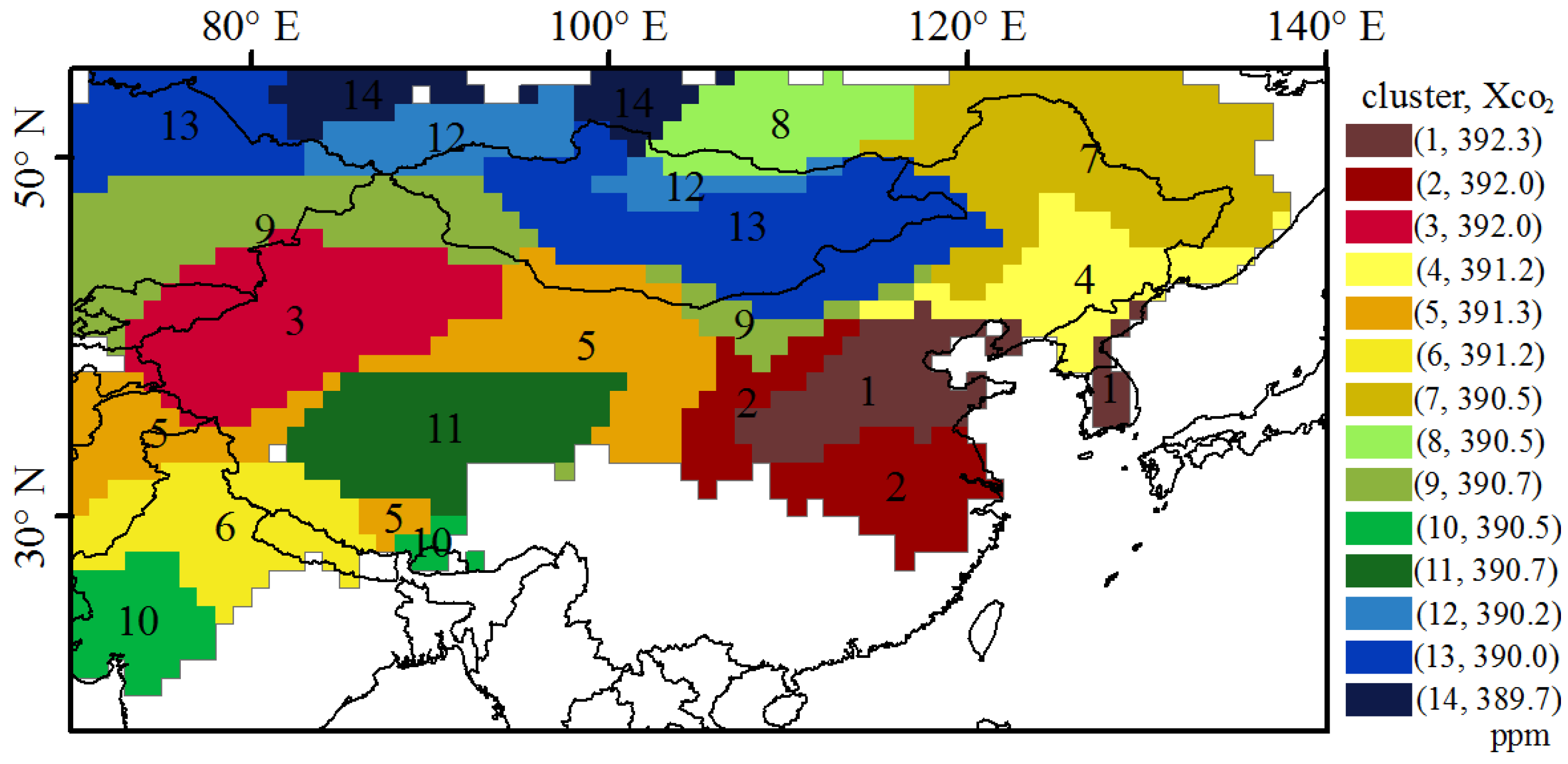
2.2. Clustering Approach Based on Multi-Temporal Xco2 Data

To make use of the temporally changing characteristics of Xco2, we used a robust cluster method to classify Xco2 data based on the similarity of CO2 concentrations to temporally changing patterns. K-means is an iterative algorithm used to partition the given dataset into k clusters, where k is a user-specified number [46,47]. The clustering result should meet the conditions that the intra-cluster similarity is high, while the inter-cluster similarity is low. The clustering process was implemented in the following steps:
(1) Combine multi-temporal Xco2 into a characteristic vector x for each spatial grid cell. The count of the grid cells is n, and “Z-score” measures are used to remove seasonality from the data. “Z-score” is a distance measure of a data point from the mean in terms of the standard deviation, and can be used for standardizing the original data [48];
(2) Randomly select k objects from n grid cells as the initial cluster centroids. The characteristic vector of cluster Ci can be expressed as mi;
(3) Assign or reassign each grid cell to the cluster to which the grid cell is the most similar based on the Euclidean distance criterion (Equation (1)) between the grid cell and cluster;
d i s ( x , C i ) = x - m i 2
(4) Update the cluster centroids by averaging characteristic vector of the grid cells for each cluster;
(5) Repeat Steps (3) and (4) until the sum of square error criterion (Equation (2)) converges when the cluster centroids do not change.
S S E = i = 1 k x C i ( d i s ( x , C i ) ) 2
Because the results of k-means clustering can be influenced by the initial cluster centroids, and the sum of square error (Equation (2)) may fall into the local optimum, the clustering process is repeated for ten times. In addition, the lowest value of SSE was chosen for acquiring stable clustering results.
To test the effects of different time intervals of the mapping Xco2 dataset, we respectively used both the M-Xco2 and S-Xco2 to the clustering process described above. Grid cells with similar Xco2 temporal patterns could be merged to respectively generate the clustering results for different k (from 3 to 40), in which month-interval clustering results are referred to as M-Clusters and season-interval clustering results are referred to as S-Clusters.
With the increase in cluster number k from 3 to 40, the averages, standard deviations, and non-negative ratios of silhouette values are calculated as measures of how appropriately the data has been clustered. Silhouette values [50,51] are used for validating the clustering results [49,50]. The silhouette is a measure of how similar each grid cell in one cluster is to grid cells in the neighboring clusters. It is given by
s ( x ) = b ( x ) a ( x ) max { a ( x ) , b ( x ) }
where a(x) is the average distance from x to all other grid cells in the same cluster, and b(x) is the minimum average distance from x to grid cells in any other clusters. s(x) ranges from −1 to +1. If s(x) is close to −1, it indicates that the clustering of x is incorrect and it should be belonged to its neighboring cluster. In contrast, if s(x) is close to 1, the current cluster is suitable for x.

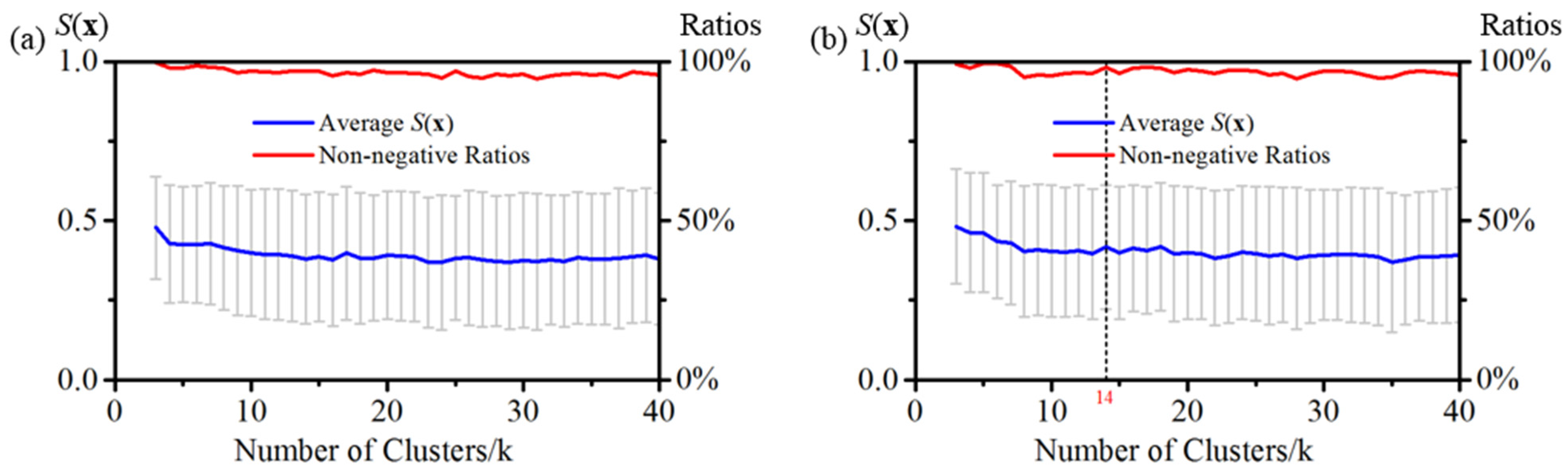
2.3. Optimal Number of Clusters

To validate cluster results and choose the best cluster parameters, the numerical evaluation indicators, including average silhouette values, and non-negative ratios of the silhouette values were used. Figure 1 shows the variations of the averages and ratios of s(x), in which the number of clusters k range from 3 to 40. The error bars represent one standard deviation of the silhouette values. The plots show that the incorrect results of the clustering ratios are limited at a low level and that the clustering results are valid for either M-Clusters or S-Clusters. Specifically, the averages remain at approximately 0.4; the standard deviations are approximately the same; and all the ratios are above 95%. Based on Figure 1a,b, we found S-Clusters are slightly better than M-Clusters.
Figure 1. Averaged silhouette values and non-negative ratios of silhouette values based on clustering results of: (a) M-Cluster; (b) S-Cluster.
Atmosphere 06 01695 g001
On the other hand, auxiliary data of emissions and absorption were used for proving the effectiveness of the clustering approach. The average and amplitude were considered the two most typical characters of temporal Xco2 variations. Before clustering, we calculated the correlation coefficients: Ravg_e between the Xco2 average and emission, Ravg_n between the Xco2 average and NPP, and Ramp_e between the Xco2 amplitude and emission. In addition, we calculated the correlation coefficient Ramp_n between the Xco2 amplitude and NPP based on gridded data, which are introduced in Section 2. Ravg_e, Ravg_n, Ramp_e, and Ramp_n results were 0.32, 0.26, 0.13, and 0.52, respectively. These results show that it is difficult to directly obtain and quantify spatial distributions of CO2 emissions using Xco2 data in a grid scale. Moreover, it is obvious that the NPP, which is representative of the absorption capability, showed a relatively strong influence on the Xco2 temporal fluctuation.
After clustering, the new Ravg_e and Ramp_n in the cluster region scale based on the clustering result were also calculated. They are illustrated in Figure 2. As shown in the figure, these correlation coefficients continuously remain at a relatively high level when k ranges from 3 to 40, although there is a slight decrease associated with the increase of k when a linear or logarithmic model is used. These results respectively prove the strong positive correlations in the cluster scale between Xco2 averages and CO2 emissions, and between Xco2 amplitudes and NPP. Compared to the analysis results before clustering, these results reveal the distribution information on both anthropogenic emissions and NPP.
In general, these results show that the satellite-based observations are correlated with regional CO2 emissions and NPP in a cluster region scale, and that the regional division by temporal clustering plays a role in exploring these relationships. The regional Xco2 averages can be regarded as a potential indicator to quantify the diversity of CO2 emissions intensity in the cluster region scale, while regional Xco2 amplitudes can be regarded as a potential indicator for analyzing NPP.
In addition, p-values were calculated in correlation analyses and applied in significance tests. Here, “p-value” is used for testing the null hypothesis of no correlation against the alternative that there is a nonzero correlation. As shown in Figure 2, where k is greater than 10, the p-values are less than 0.05, and the correlation analysis results can be considered reliable. Based on the above results and analyses, k can be appropriately chosen from the range of 10 to 40, and average silhouette values and non-negative ratios reach their peak when k is equal to 14 in S-Clusters when the minimum standard deviation is reached. Therefore, k = 14 in S-Clusters (average = 0.417, SD = 0.195, and ratio = 98.014%) is regarded as the optimal clustering scheme, and will be described and analyzed in more detail further.
Figure 2. Correlation analysis: (a) Ravg_e between the Xco2 average and CO2 emissions based on the clustering results; (b) Ramp_n between the Xco2 amplitude and NPP based on the clustering results.
Atmosphere 06 01695 g002

3. Results and Discussion

Figure 3 presents the results of 14 clusters obtained using the clustering method described in Section 2.2, and the mean Xco2 in each clusters. As shown in the figure, Xco2 data of Clusters 1 and 2 in Central and Eastern China are the maximum, followed by those of Cluster 3 in Xinjiang province in Western China. Xco2 data of Clusters 12, 13, and 14, located around Inner Mongolia, Mongolia, Northeastern Kazakhstan, are the minimum.
Figure 3. Clustering result based on S-Xco2 dataset with 14 clusters and the corresponding cluster-averaged Xco2 data from 2010 to 2012.
Atmosphere 06 01695 g003

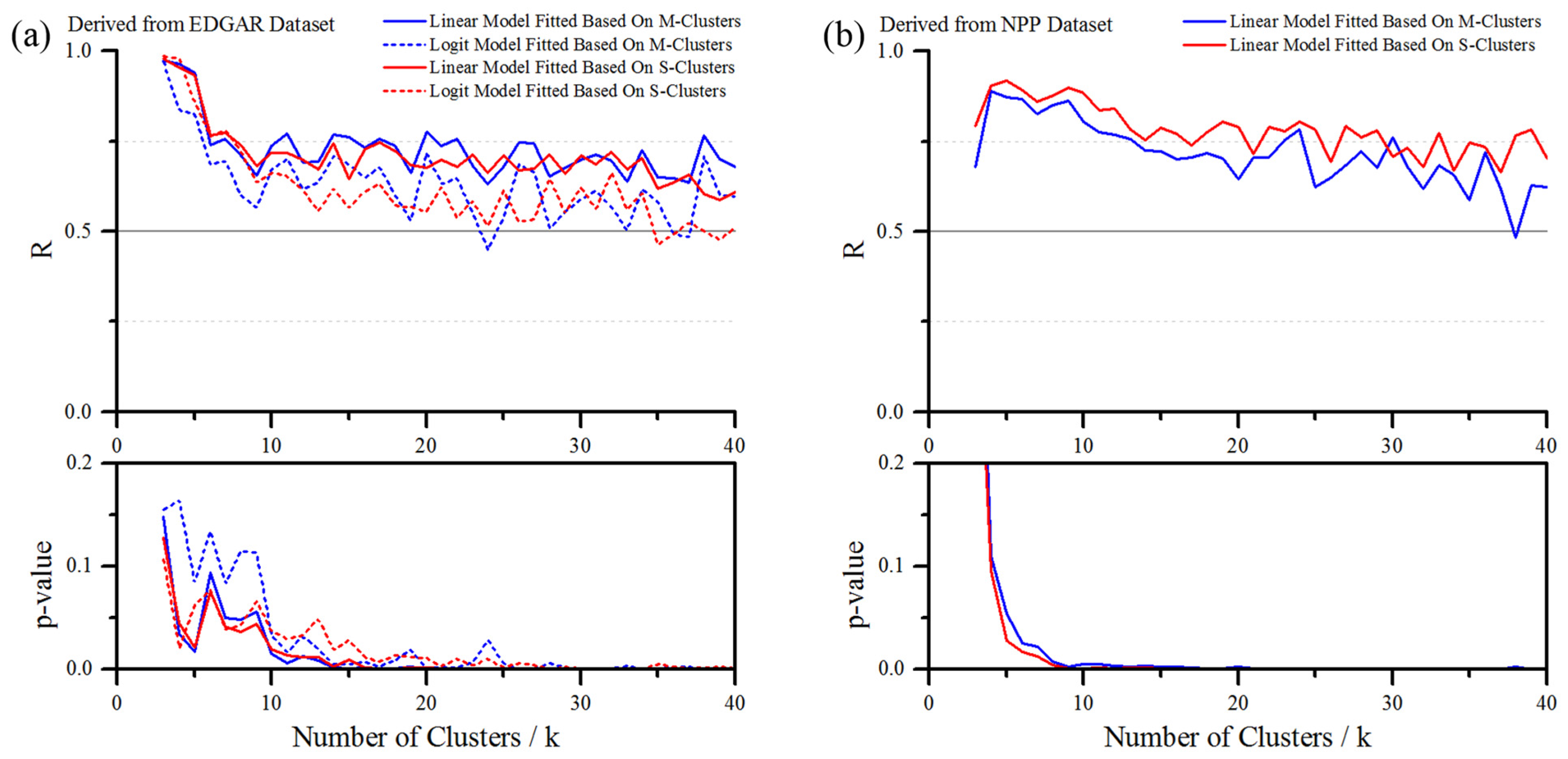
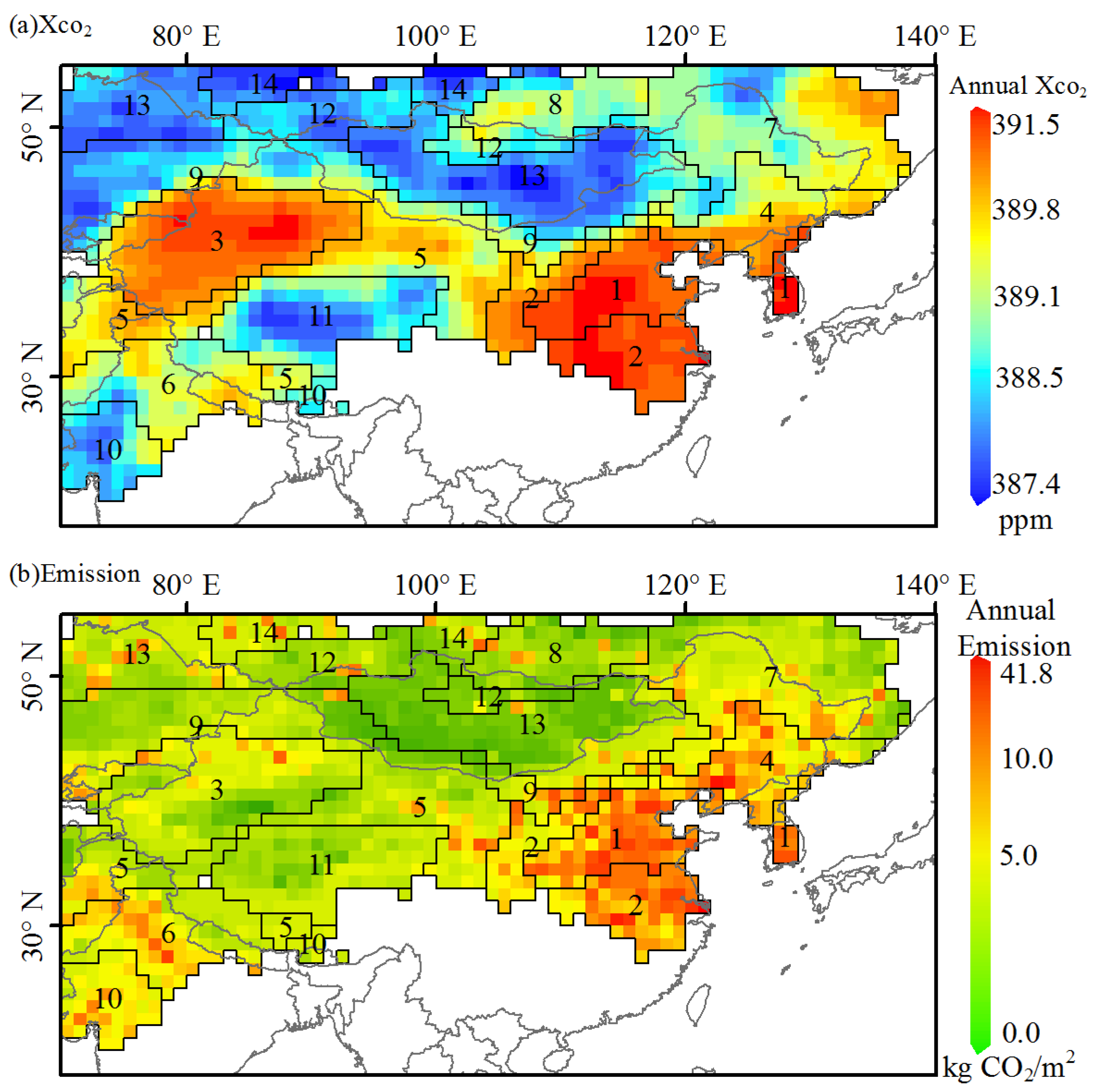
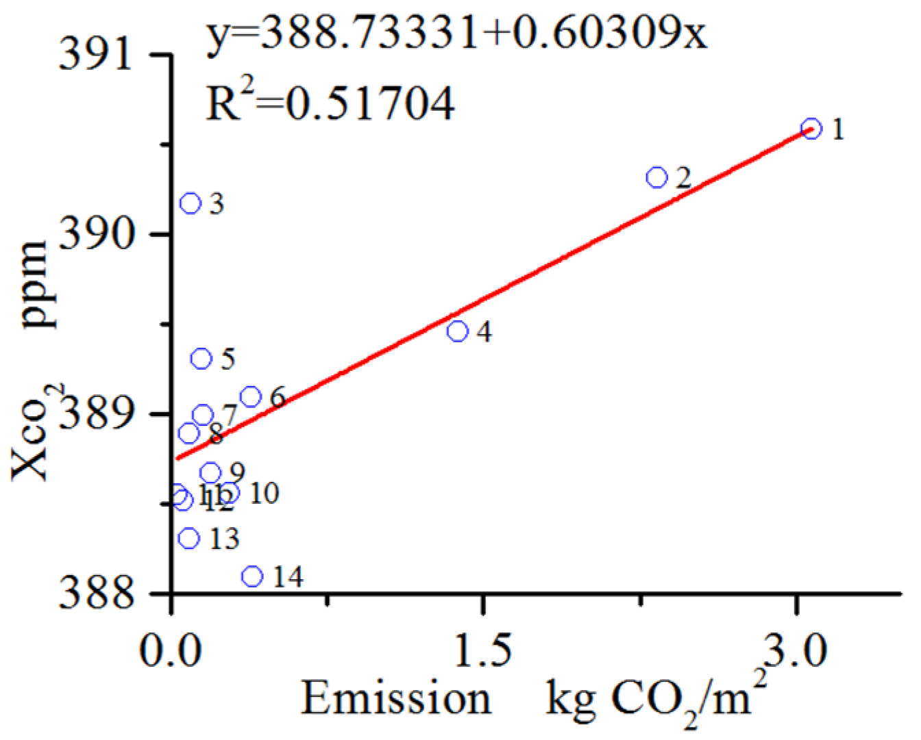
3.1. Xco2 and Anthropogenic Emissions
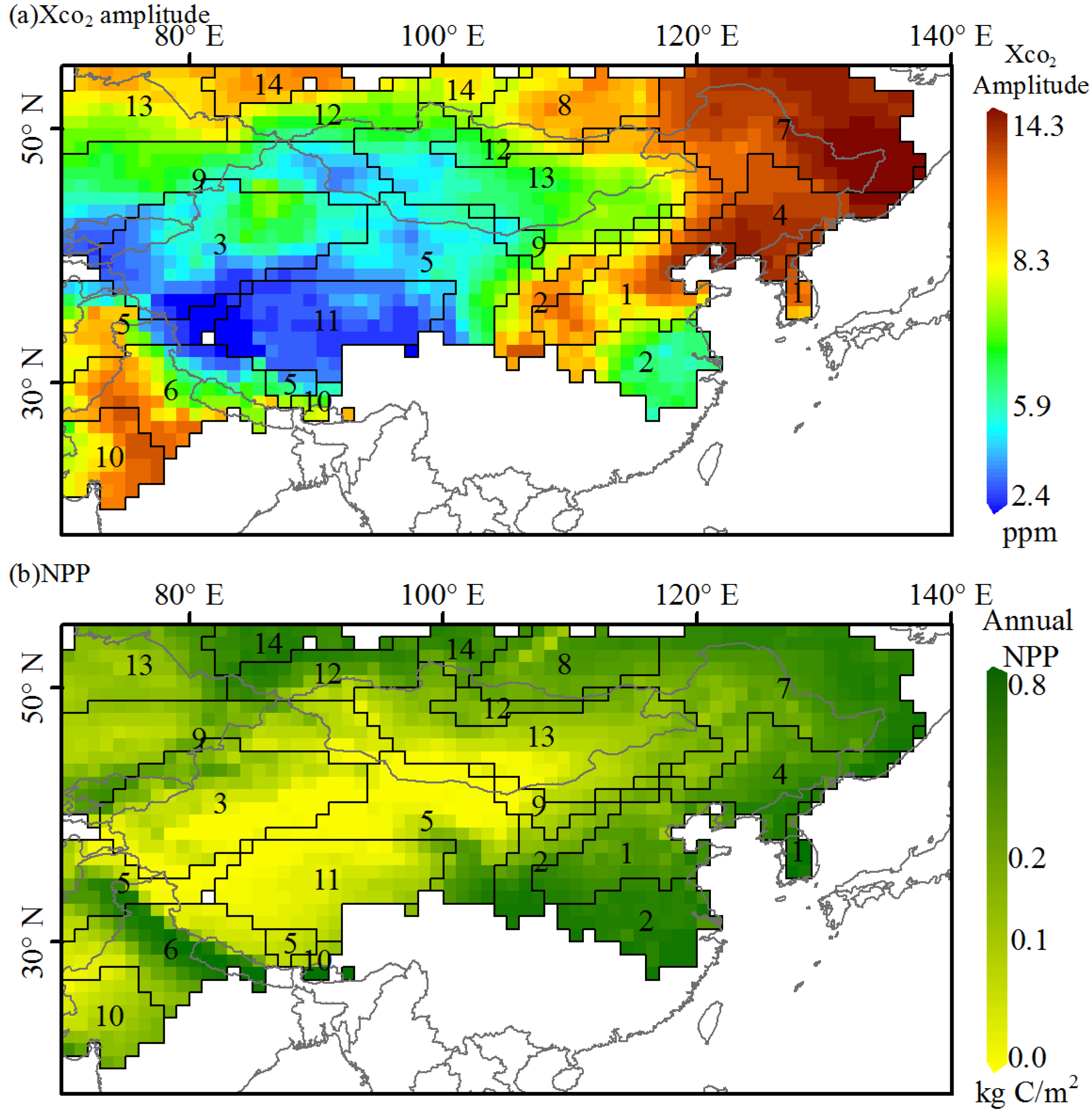
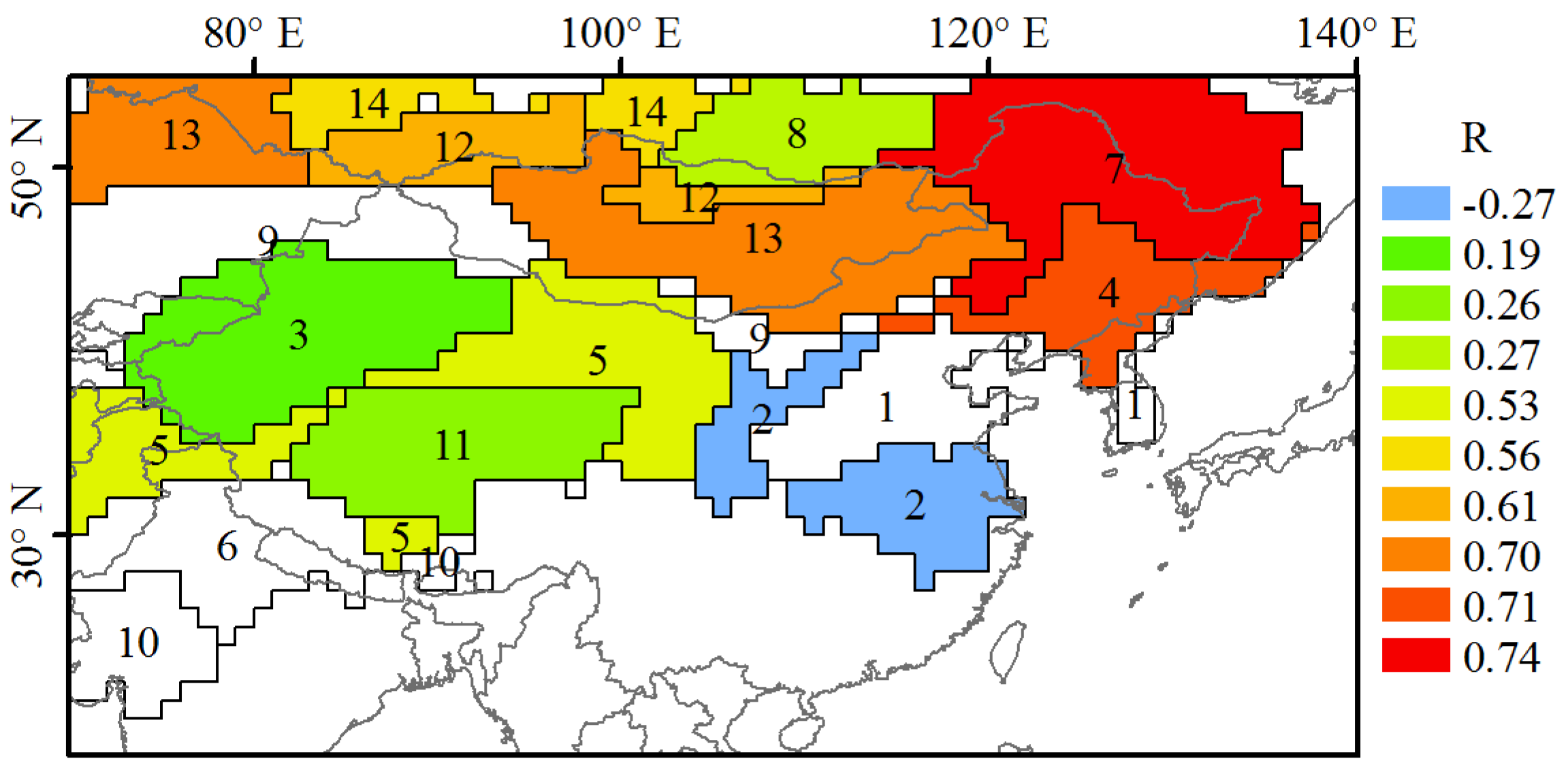
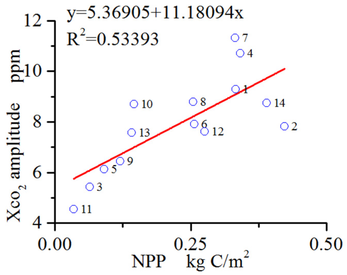
Based on the optimal clustering result shown in Figure 3, an overlay analysis with CO2 concentrations and emission data, respectively, is implemented. Figure 4a,b show annual Xco2 and CO2 emissions in 2010 overlaid with polylines of the 14 clusters. Figure 4b is the average of CO2 emissions in 1° × 1° grid cells derived from original emission data; the emission units are converted to kg CO2/m2.
Figure 4. (a) Annual Xco2; (b) Annual CO2 emissions in 2010 overlapped with the optimal cluster result (black lines).
Atmosphere 06 01695 g004
From a comparison of the spatially distributed borders of clusters shown in Figure 4a with emissions in Figure 4b, it is obvious that the areas of Clusters 1, 2, and 4 with large Xco2 values coincide with high emissions, whereas Clusters 11, 12, and 13 with small Xco2 values correspond to the low emission areas in Mongolia, part of Inner Mongolia and Xizang in China. The exception is Cluster 3, located in Xinjiang province in western China, where Xco2 is very high but emissions are not.
Figure 5. Regression analysis between cluster-averaged CO2 emissions and Xco2 in 2010.
Atmosphere 06 01695 g005
In addition, Figure 5 depicts a correlation between Xco2 and CO2 emissions. The results indicate that a positive correlation is shown between emissions and Xco2 at the clustering region scale. Xco2 of Cluster 3, an outlier in Figure 5, is abnormally high but low in emissions.

3.2. Xco2 and NPP

The seasonal changes of CO2 concentrations are mainly caused by vegetation absorptions. The amplitude of seasonal variations in a year depends on vegetation coverage and growth activities in the northern parts of the northern hemisphere [51,52,53]. Figure 6a presents the seasonal amplitude of Xco2 in 2010, which is calculated by the difference between the maximum and minimum of the monthly averaged Xco2 of each grid cell. Figure 6b presents the annual mean NPP in 2010 of each grid cell, which can indicate the ability of vegetation to absorb CO2. Figure 6b is the average of CO2 fluxes in 1° × 1° grid cells derived from original NPP data.
Figure 6. (a) Seasonal amplitude of Xco2; (b) grid map of annual NPP in 2010 overlapped with the optimal cluster result (black lines).
Atmosphere 06 01695 g006
It is evident that the spatial distribution of Xco2 amplitudes are generally in agreement with the spatial trend of NPP. Clusters 1, 4, 7, and 14 with large amplitudes of Xco2 show significant corresponds to high NPP, while Clusters 3, 5, and 11 with small amplitudes of Xco2 demonstrate low NPP. This indicates that the impact of NPP, a measurement of vegetation activities, on the seasonal changing amplitudes of Xco2.
The correlation coefficients between seasonal amplitudes of Xco2 and NPP for each cluster are shown in Figure 7. It is shown that correlations between the Xco2 amplitude and NPP are mostly positive; moreover, the larger NPP is, the higher the correlation coefficient is, except for Clusters 1 and 2, which are the maximum emission areas (shown in Figure 4b), and Cluster 9.
Figure 7. Correlation coefficients (R) of all clustering classes (p-value < 0.05) between the Xco2 amplitude and NPP.
Atmosphere 06 01695 g007
Regression analysis between the cluster-averaged NPP and Xco2 amplitude is shown in Figure 8. The coefficient of determination between them is 0.53 for all clusters, which is similar to the coefficient of determination (r2 = 0.52) between Xco2 and the emissions (shown in Figure 5). The results imply that the variations of Xco2 can be equally explained by the underlying anthropogenic emissions and vegetation absorptions in the whole study area.
Figure 8. Regression analysis between cluster-averaged NPP and Xco2 amplitude in 2010.
Atmosphere 06 01695 g008

3.3. Attribution of Xco2 Clusters

Figure 9 shows the variation of the monthly mean Xco2 in each cluster. As is shown, each cluster demonstrates a different seasonal changing pattern of Xco2. Clusters 7, 8, 12, and 14 located at the northern part present two high Xco2 peaks, which may be caused by vegetation growth activity and temperature variations. On the other hand, Clusters 3, 5, and 11 show smaller seasonal amplitudes, which can be attributed to sparse vegetation areas in these study regions.
Figure 9. Variation of monthly averaged Xco2 in each Cluster (number of clusters k = 14). Blue, green, and red lines correspond to average, minimum, and maximum Xco2 values in each cluster, respectively, derived from the gap-filled Xco2 dataset. Error bars represent one standard deviation of Xco2, and the grey scatter points correspond to original observations from the ACOS-Xco2 dataset.
Atmosphere 06 01695 g009
Table 1 demonstrates typical statistics of Xco2 and auxiliary data in each cluster, including Xco2 variations, anthropogenic emissions, and NPP. The contrast of Xco2 in Table 1 is calculated by subtracting the average Xco2 of the study area (389.10 ppm) from cluster-averaged Xco2 to indicate the difference from the regional background Xco2 value in each cluster. Xco2 amplitude is calculated by the maximum monthly cluster-averaged Xco2 minus the corresponding minimum in each cluster. The strength of emissions is derived from the emissions in the target cluster divided by the maximum emission value of all clusters (Cluster 1). The strength of NPP is calculated in the same way.
The fraction of land cover is the fraction of low vegetation (L), forest (F), and non-vegetated areas (N), in each cluster derived from land cover data. The correlation coefficients (p-value < 0.05) of the Xco2 amplitude versus the NPP of all grid cells within a cluster are also listed in this table. The correlation between Xco2 and emissions of all grid cells within a cluster is very small and not significant, and is therefore not listed in Table 1.
Table 1. Attribute characteristics of each cluster from the 2010 data.
ClusterContrast of Xco2
ppm
Xco2 Amplitude
ppm
Ramp_n Xco2 Amplitude vs. NPPStrength of EmissionStrength of NPPFraction of Land Cover*
L:F:N
Types
11.59.3-1.000.7970:22:4E
21.27.8−0.270.761.0068:27:2E
31.15.40.190.030.1538:1:60Δ
40.410.70.710.450.8158:38:1-
50.26.10.530.050.2238:2:59-
60.07.9-0.130.6169:10:20-
7−0.111.30.740.050.7851:48:0.5A
8−0.28.80.270.030.6044:49:0.5-
9−0.46.4-0.060.2979:0.5:19-
10−0.58.7-0.090.3489:5:5-
11−0.54.60.260.010.0856:-:42-
12−0.67.60.610.020.6572:26:0.5A
13−0.87.60.700.030.3385:2:12A
14−1.008.70.560.130.9253:45:0.5A
* The land cover types “grasses/cereal”, “shrubs”, “broadleaf crops” and “savanna” were grouped into type “L”; “evergreen broad-leaf forest”, “deciduous broadleaf forest”, “evergreen needleleaf forest” and “deciduous needle-leaf forest” were grouped into type “F”; “unvegetated” and “urban” areas were grouped into type “N”.
In this section, the anthropogenic emissions and vegetation absorptions described in Section 3.1 and Section 3.2, and the seasonal changing patterns of Xco2 of each cluster shown in Figure 9, will be combined to analyze the attribute characteristics of the 14 clusters listed in Table 1. As a result, the 14 clusters can be divided into three flux types, as outlined below.
(1) Strong Emission Type: Clusters 1 and 2
Clusters 1 and 2 as a group, strongly tends to present sources regions as they show the highest Xco2 (390.6 ppm and 390.3 ppm in average, as shown in Table 1), and the largest positive contrast (1.5 ppm and 1.2 ppm). It can be known from bottom-up investigation of carbon emissions (EDGAR) that in these two cluster regions there are very intensive big power fuel plants and dense populations which corresponds to large emissions (Table 1). The strong anthropogenic emissions can disturb the temporal variations of Xco2. Consequently, the correlations between the Xco2 amplitude and NPP do not show a significant correlation although they show a large Xco2 amplitude (9.3 ppm and 7.8 ppm), which is likewise due to vegetation coverage of more than 90% in these regions.
These results indicate that both Clusters 1 and 2 can be attributed to a source with strong emissions. These clusters show different temporal variations of Xco2 (Figure 9), even if both of them belong to the strong emission type. Cluster 1 is located in the major grain producing areas mixed with many residential areas in China. Intensive farming and crop vegetation growth have resulted in a significant seasonal amplitude of Xco2 (9.3 ppm in Table 1) due to crop CO2 absorption. Temporal variations of Xco2 show that Xco2 sharply increased from August to October over this cluster compared with Cluster 2, which is likely due to the crops being harvested and large amounts of straw being burned during this period. Cluster 2, located at the paddy fields mixed with the fragmented forests, residential areas, shows that a 7.8 ppm of Xco2 amplitude, which is slightly less than that in Cluster 1. Their different temporally changing patterns of Xco2 indicate the effects of different anthropogenic emitting actions on variations of Xco2.
(2) Strong Absorption Type: Clusters 7, 12, 13, and 14
Clusters 7, 12, 13, and 14, as a group, tend to be strong sinks, according to the negative contrasts and strong correlations between Xco2 and NPP, high fractions of vegetation, and less anthropogenic emissions shown in Table 1. Xco2 values over these cluster regions are lower than the overall average; moreover, the contrasts are −0.1 ppm, −0.6 ppm, −0.8 ppm, and −1.0 ppm, respectively (Table 1). These clusters are located at north of latitude 45°N, and are covered with dense vegetation and forest. Accordingly, the correlations between Xco2 amplitudes and NPP are significantly larger than 0.55 over these clusters. This demonstrates the effects of vegetation absorption on Xco2 variations. With strong vegetation absorptions in addition to low anthropogenic emissions over these clusters (Figure 4), they tend to be sinks of atmospheric CO2. These clusters show different temporally changing patterns of Xco2 (Figure 9), which demonstrate the effects of vegetation absorption. Among the clusters, Clusters 7 and 14 show the highest amplitude of Xco2 seasonal variation (11.3 ppm and 8.7 ppm, respectively, shown in Table 1), which is likely induced by the highest coverage of mixed broad-leaf with needle-leaf forest. Clusters 12 and 13 show a strong correlation between Xco2 amplitude and NPP, which is 0.61 and 0.70, respectively, although they have less forest coverage and a high fraction of grasslands. The values of Xco2 over these clusters as shown in Figure 9, moreover, are almost unchanged from October to January, or they present a low peak around December, which is likely due to the low temperature in the high latitude region.
(3) Tending to Balance Type: Clusters 4, 5, 6, 8, 9, 10 and 11
Clusters 4, 5, 6, 8, 9, 10 and 11 are defined as being a “tending to balance” type. All of their mean Xco2 values are close to the average level of the whole study area. In addition, Clusters 5, 6, 8, 9, 10 and 11 do not show significant correlations between Xco2 amplitude and NPP, and there are the small anthropogenic emissions over these regions. Cluster 4 shows slightly higher Xco2 than the average level, with a 0.4 ppm contrast, mainly due to significant large anthropogenic emission. However, the correlation between the Xco2 amplitude and NPP is 0.71, which implies that the CO2 enhancement from the anthropogenic emission may be in equilibrium with the vegetation absorption. Cluster 11, located on the Qinghai-Tibet Plateau, shows lower Xco2 amplitude than the other regions, which are probably owing to its low NPP and high altitude.
Cluster 3 is indistinctly grouped as its abnormally high Xco2 while there is less anthropogenic emissions (Figure 4). Cluster 3, located at a desert area in China, shows high Xco2 values, which are likely owing to uncertainties of Xco2 retrievals from satellite over these high lightness desert [9], and further verification is needed in this region.

4. Conclusions

In this paper, a k-means cluster analysis method based on the temporally changing features of Xco2 was proposed for application to the gap-filled ACOS Xco2 dataset to view spatial pattern of CO2 emissions and absorption in Central-Eastern Asia. 14 clusters were obtained by optimizing the clustering results and evaluated using the characteristics of Xco2 variations combined with emissions data, NPP data, and land cover data. The clustering result demonstrates that each cluster can be related to the typical features of anthropogenic emissions and vegetation absorptions.
The relationships between seasonal variations of Xco2, and underlying anthropogenic emissions and vegetation absorption were analyzed respectively. Cluster-averaged Xco2 tend to correlate with regional emissions, while seasonal amplitude of Xco2 is highly related to vegetation NPP. Strong anthropogenic emissions may disturb the relationship between the seasonal amplitude of Xco2 and NPP data. Consequently, the 14 clusters can be divided into three types: strong emission, strong absorption, and a “tending to balance” type. Different clusters, corresponding to different temporally changing patterns of Xco2, indicate that the Xco2 values increase with anthropogenic activities and that Xco2 reduction is caused by vegetation absorption on a regional scale.
This study shows that the developed cluster-analysis approach based on temporal variation of Xco2 can effectively provide a way to reveal the spatial patterns of underlying anthropogenic emissions and vegetation absorptions, and therefore enable to us to better understand how the seasonally changing pattern of CO2 concentrations is affected by anthropogenic emissions and vegetation absorptions. The result of clustering can provide the significant monitoring targets of anthropogenic emissions and vegetation absorption to support the implement of regional emissions reduction of carbon.

Acknowledgments

This research was supported by the “Strategic Priority Research Program—Climate Change: Carbon Budget and Relevant Issues” of the Chinese Academy of Sciences, Grant No. XDA05040401, and the National High Technology Research and Development Program of China (2012AA12A301). The authors are immensely grateful to the anonymous reviewers and editor for their excellent, valuable comments. The ACOS-GOSAT v3.3 data were produced by the ACOS/OCO-2 project at the Jet Propulsion Laboratory, California Institute of Technology, and were obtained from the ACOS/OCO-2 data archive maintained at the NASA Goddard Earth Science Data and Information Services Center. We would also like to acknowledge the GOSAT Project for acquiring the spectra, and the EDGAR data (http://edgar.jrc.ec.europa.eu/) provided by the joint project of the European Commission Joint Research Center (JRC) and the Netherlands Environmental Assessment Agency (PBL). We also acknowledge that the Terra MODIS GPP/NPP Product (MOD17A3) and Land Cover Type Climate Modeling Grid (CMG) product (MCD12C1) were retrieved from the online Data Pool, courtesy of the NASA Land Processes Distributed Active Archive Center (LP DAAC), USGS/Earth Resources Observation and Science (EROS) Center, Sioux Falls, South Dakota, https://lpdaac.usgs.gov/data_access/data_pool.

Author Contributions

Da Liu and Liping Lei conceived and designed the experiments; Da Liu performed the experiments; Da Liu and Liping Lei analyzed the data; Lijie Guo contributed materials; and Da Liu, Liping Lei, and Zhaocheng Zeng wrote the paper.

Conflicts of Interest

The authors declare no conflicts of interest.

References

  1. Falkowski, P.; Scholes, R.J.; Boyle, E.; Canadell, J.; Canfield, D.; Elser, J.; Gruber, N.; Hibbard, K.; Hogberg, P.; Linder, S.; et al. The global carbon cycle: A test of our knowledge of earth as a system. Science 2000, 290, 291–296. [Google Scholar] [CrossRef] [PubMed]
  2. Canadell, J.G.; Le Quere, C.; Raupach, M.R.; Field, C.B.; Buitenhuis, E.T.; Ciais, P.; Conway, T.J.; Gillett, N.P.; Houghton, R.A.; Marland, G. Contributions to accelerating atmospheric CO2 growth from economic activity, carbon intensity, and efficiency of natural sinks. Proc. Natl. Acad. Sci. USA 2007, 104, 18866–18870. [Google Scholar] [CrossRef] [PubMed]
  3. Raupach, M.R.; Marland, G.; Ciais, P.; Le Quere, C.; Canadell, J.G.; Klepper, G.; Field, C.B. Global and regional drivers of accelerating CO2 emissions. Proc. Natl. Acad. Sci. USA. 2007, 104, 10288–10293. [Google Scholar] [CrossRef] [PubMed]
  4. Ciais, P.; Sabine, C.; Bala, G.; Bopp, L.; Brovkin, V.; Canadell, J.; Chhabra, A.; DeFries, R.; Galloway, J.; Heimann, M.; et al. Carbon and other biogeochemical cycles. In Climate Change 2013: The Physical Science Basis. Contribution of Working Group I to the Fifth Assessment Report of the Intergovernmental Panel on Climate Change; Stocker, T.F., Qin, D., Plattner, G.-K., Tignor, M., Allen, S.K., Boschung, J., Nauels, A., Xia, Y., Bex, V., Midgley, P.M., Eds.; Cambridge University Press: Cambridge, UK; New York, NY, USA, 2013; pp. 465–570. [Google Scholar]
  5. Chevallier, F.; Maksyutov, S.; Bousquet, P.; Breon, F.-M.; Saito, R.; Yoshida, Y.; Yokota, T. On the accuracy of the CO2 surface fluxes to be estimated from the GOSAT observations. Geophys. Res. Lett. 2009. [Google Scholar] [CrossRef]
  6. Frankenberg, C.; Fisher, J.B.; Worden, J.; Badgley, G.; Saatchi, S.S.; Lee, J.-E.; Toon, G.C.; Butz, A.; Jung, M.; Kuze, A.; et al. New global observations of the terrestrial carbon cycle from GOSAT: Patterns of plant fluorescence with gross primary productivity. Geophys. Res. Lett. 2011. [Google Scholar] [CrossRef]
  7. Morino, I.; Uchino, O.; Inoue, M.; Yoshida, Y.; Yokota, T.; Wennberg, P.O.; Toon, G.C.; Wunch, D.; Roehl, C.M.; Notholt, J.; et al. Preliminary validation of column-averaged volume mixing ratios of carbon dioxide and methane retrieved from GOSAT short-wavelength infrared spectra. Atmos. Meas. Tech. 2011, 4, 1061–1076. [Google Scholar] [CrossRef]
  8. Wei, J.; Savtchenko, A.; Vollmer, B.; Hearty, T.; Albayrak, A.; Crisp, D.; Eldering, A. Advances in CO2 observations from airs and acos. IEEE Geosci. Remote Sens. Lett. 2014, 11, 891–895. [Google Scholar] [CrossRef]
  9. O’Dell, C.W.; Connor, B.; Boesch, H.; O’Brien, D.; Frankenberg, C.; Castano, R.; Christi, M.; Crisp, D.; Eldering, A.; Fisher, B.; et al. The ACOS CO2 retrieval algorithm—Part 1: Description and validation against synthetic observations. Atmos. Meas. Tech. 2012, 5, 99–121. [Google Scholar] [CrossRef]
  10. Schneising, O.; Buchwitz, M.; Reuter, M.; Heymann, J.; Bovensmann, H.; Burrows, J.P. Long-term analysis of carbon dioxide and methane column-averaged mole fractions retrieved from SCIAMACHY. Atmos. Chem. Phys. 2011, 11, 2863–2880. [Google Scholar] [CrossRef]
  11. Yoshida, Y.; Ota, Y.; Eguchi, N.; Kikuchi, N.; Nobuta, K.; Tran, H.; Morino, I.; Yokota, T. Retrieval algorithm for CO2 and CH4 column abundances from short-wavelength infrared spectral observations by the greenhouse gases observing satellite. Atmos. Meas. Tech. 2011, 4, 717–734. [Google Scholar] [CrossRef]
  12. Yokota, T.; Yoshida, Y.; Eguchi, N.; Ota, Y.; Tanaka, T.; Watanabe, H.; Maksyutov, S. Global concentrations of CO2 and CH4 retrieved from GOSAT: First preliminary results. Sola 2009, 5, 160–163. [Google Scholar] [CrossRef]
  13. Connor, B.J.; Boesch, H.; Toon, G.; Sen, B.; Miller, C.; Crisp, D. Orbiting carbon observatory: Inverse method and prospective error analysis. J. Geophys. Res. - Atmos. 2008. [Google Scholar] [CrossRef]
  14. Yoshida, Y.; Eguchi, N.; Ota, Y.; Kikuchi, N.; Nobuta, K.; Aoki, T.; Yokota, T. Algorithm theoretical basis document (ATBD) for CO2 and CH4 column amounts retrieval from GOSAT TANSO-FTS SWIR; NIES, GOSAT project Document (NIES-GOSAT-PO-014) Version 1.0, 2010. Available online: http://data.gosat.nies.go.jp/GosatUserInterfaceGateway/guig/doc/documents/ATBD_FTSSWIRL2_V1.1_en.pdf (accessed on 5 November 2015).
  15. Crisp, D.; Fisher, B.M.; O’Dell, C.; Frankenberg, C.; Basilio, R.; Boesch, H.; Brown, L.R.; Castano, R.; Connor, B.; Deutscher, N.M.; et al. The ACOS CO2 retrieval algorithm—Part ii: Global Xco2 data characterization. Atmos. Meas. Tech. 2012, 5, 687–707. [Google Scholar] [CrossRef]
  16. Feng, L.; Palmer, P.I.; Boesch, H.; Dance, S. Estimating surface CO2 fluxes from space-borne CO2 dry air mole fraction observations using an ensemble kalman filter. Atmos. Chem. Phys. 2009, 9, 2619–2633. [Google Scholar] [CrossRef]
  17. Hamazaki, T.; Kuze, A.; Kondo, K. Sensor system for greenhouse gas observing satellite (GOSAT). In Proceedings of SPIE 5543, Infrared Spaceborne Remote Sensing XII, Bellingham, WA, USA, 4 November 2004; pp. 275–282.
  18. Hamazaki, T.; Kaneko, Y.; Kuze, A.; Kondo, K. Fourier transform spectrometer for Greenhouse Gases observing satellite (GOSAT). In Proceedings of SPIE 5659, Enabling Sensor and Platform Technologies for Spaceborne Remote Sensing, Bellingham, WA, USA, 18 January 2005; pp. 73–80.
  19. Oshchepkov, S.; Bril, A.; Yokota, T. PPDF-based method to account for atmospheric light scattering in observations of carbon dioxide from space. J. Geophys. Res. - Atmos. 2008. [Google Scholar] [CrossRef]
  20. Hungershoefer, K.; Breon, F.M.; Peylin, P.; Chevallier, F.; Rayner, P.; Klonecki, A.; Houweling, S.; Marshall, J. Evaluation of various observing systems for the global monitoring of CO2 surface fluxes. Atmos. Chem. Phys. 2010, 10, 10503–10520. [Google Scholar] [CrossRef]
  21. Butz, A.; Guerlet, S.; Hasekamp, O.; Schepers, D.; Galli, A.; Aben, I.; Frankenberg, C.; Hartmann, J.M.; Tran, H.; Kuze, A.; et al. Toward accurate CO2 and CH4 observations from GOSAT. Geophys. Res. Lett. 2011. [Google Scholar] [CrossRef]
  22. Wunch, D.; Wennberg, P.O.; Toon, G.C.; Connor, B.J.; Fisher, B.; Osterman, G.B.; Frankenberg, C.; Mandrake, L.; O’Dell, C.; Ahonen, P.; et al. A method for evaluating bias in global measurements of CO2 total columns from space. Atmos. Chem. Phys. 2011, 11, 12317–12337. [Google Scholar] [CrossRef]
  23. Qu, Y.; Zhang, C.M.; Wang, D.Y.; Tian, P.B.; Bai, W.G.; Zhang, X.Y.; Zhang, P.; Dai, H.S.; Wu, Q.M. Comparison of atmospheric CO2 observed by GOSAT and two ground stations in China. Int. J. Remote Sens. 2013, 34, 3938–3946. [Google Scholar] [CrossRef]
  24. Lei, L.; Guan, X.; Zeng, Z.; Zhang, B.; Ru, F.; Bu, R. A comparison of atmospheric CO2 concentration GOSAT-based observations and model simulations. Sci. Chin.-Earth Sci. 2014, 57, 1393–1402. [Google Scholar] [CrossRef]
  25. Belikov, D.A.; Bril, A.; Maksyutov, S.; Oshchepkov, S.; Saeki, T.; Takagi, H.; Yoshida, Y.; Ganshin, A.; Zhuravlev, R.; Aoki, S.; et al. Column-averaged CO2 concentrations in the subarctic from GOSAT retrievals and NIES transport model simulations. Polar Sci. 2014, 8, 129–145. [Google Scholar] [CrossRef]
  26. Wang, X.; Zhang, X.Y.; Zhang, L.Y.; Gao, L.; Tian, L. Interpreting seasonal changes of low-tropospheric CO2 over china based on SCIAMACHY observations during 2003–2011. Atmos. Environ. 2015, 103, 180–187. [Google Scholar] [CrossRef]
  27. Maksyutov, S.; Takagi, H.; Valsala, V.K.; Saito, M.; Oda, T.; Saeki, T.; Belikov, D.A.; Saito, R.; Ito, A.; Yoshida, Y.; et al. Regional CO2 flux estimates for 2009–2010 based on GOSAT and ground-based CO2 observations. Atmos. Chem. Phys. 2013, 13, 9351–9373. [Google Scholar] [CrossRef]
  28. Deng, F.; Jones, D.B.A.; Henze, D.K.; Bousserez, N.; Bowman, K.W.; Fisher, J.B.; Nassar, R.; O’Dell, C.; Wunch, D.; Wennberg, P.O.; et al. Inferring regional sources and sinks of atmospheric CO2 from GOSAT XCO2 data. Atmos. Chem. Phys. 2014, 14, 3703–3727. [Google Scholar] [CrossRef]
  29. Ciais, P.; Rayner, P.; Chevallier, F.; Bousquet, P.; Logan, M.; Peylin, P.; Ramonet, M. Atmospheric inversions for estimating CO2 fluxes: Methods and perspectives. Clim. Change 2010, 103, 69–92. [Google Scholar] [CrossRef]
  30. Kort, E.A.; Frankenberg, C.; Miller, C.E.; Oda, T. Space-based observations of megacity carbon dioxide. Geophys. Res. Lett. 2012. [Google Scholar] [CrossRef]
  31. Keppel-Aleks, G.; Wennberg, P.O.; O’Dell, C.W.; Wunch, D. Towards constraints on fossil fuel emissions from total column carbon dioxide. Atmos. Chem. Phys. 2013, 13, 4349–4357. [Google Scholar] [CrossRef]
  32. Musdholifah, A.; Hashim, S.Z.M.; Ngah, R. Hybrid PCA-ILGC clustering approach for high dimensional data. IEEE Sys. Man. Cybern. 2012, 420–424. [Google Scholar]
  33. Deng, M.; Liu, Q.L.; Wang, J.Q.; Shi, Y. A general method of spatio-temporal clustering analysis. Sci. China Inform Sci. 2013. [Google Scholar] [CrossRef]
  34. Steinbach, M.; Tan, P.-N.; Kumar, V.; Potter, C.; Klooster, S.; Torregrosa, A. Clustering earth science data: Goals, issues and results. In Proceedings of the Fourth KDD Workshop on Mining Scientific Datasets, San Francisco, CA, USA, 26 August 2001.
  35. Steinbach, M.; Tan, P.-N.; Kumar, V.; Klooster, S.; Potter, C. Discovery of climate indices using clustering. In Proceedings of the ninth ACM SIGKDD international conference on Knowledge discovery and data mining, Washington, DC, USA, 24–27 August 2003; ACM: New York, NY, USA, 2003; pp. 446–455. [Google Scholar]
  36. Oda, T.; Maksyutov, S. A very high-resolution (1 km × 1 km) global fossil fuel CO2 emission inventory derived using a point source database and satellite observations of nighttime lights. Atmos. Chem. Phys. 2011, 11, 543–556. [Google Scholar] [CrossRef]
  37. Zhang, L.; Xiao, J.; Li, L.; Lei, L.; Li, J. China’s sizeable and uncertain carbon sink: A perspective from GOSAT. Chin. Sci. Bull. 2014, 59, 1547–1555. [Google Scholar] [CrossRef]
  38. Zeng, Z.; Lei, L.; Hou, S.; Ru, F.; Guan, X.; Zhang, B. A regional gap-filling method based on spatiotemporal variogram model of CO2 columns. IEEE Trans. Geosci. Remote Sens. 2014, 52, 3594–3603. [Google Scholar] [CrossRef]
  39. Guo, L.J.; Lei, L.P.; Zeng, Z.C.; Zou, P.F.; Liu, D.; Zhang, B. Evaluation of spatio-temporal variogram models for mapping Xco2 using satellite observations: A case study in china. IEEE J. Selected Topics in Appl. Earth Observations Remote Sens. 2015, 8, 376–385. [Google Scholar] [CrossRef]
  40. Zeng, Z.; Lei, L.; Guo, L.; Zhang, L.; Zhang, B. Incorporating temporal variability to improve geostatistical analysis of satellite-observed CO2 in China. Chin. Sci. Bull. 2013, 58, 1948–1954. [Google Scholar] [CrossRef]
  41. Osterman, G.; Eldering, A.; Avis, C.; O’Dell, C.; Martinez, E.; Crisp, D.; Frankenberg, C.; Fisher, B.; Wunch, D. ACOS 3.3 Level 2 Standard Product Data User’s Guide, v3.3; GES DISC: Greenbelt, MD, USA, 2011. [Google Scholar]
  42. Ciais, P.; Dolman, A.J.; Bombelli, A.; Duren, R.; Peregon, A.; Rayner, P.J.; Miller, C.; Gobron, N.; Kinderman, G.; Marland, G.; et al. Current systematic carbon-cycle observations and the need for implementing a policy-relevant carbon observing system. Biogeosciences 2014, 11, 3547–3602. [Google Scholar] [CrossRef] [Green Version]
  43. Olivier, J.G.J.; Janssens-Maenhout, G. Part iii: Greenhouse gas emissions: 1. Shares and trends in greenhouse gas emissions; 2. Sources and methods; total greenhouse gas emissions. In CO2 Emissions from Fuel Combustion, 2012 edition; IEA: Paris, France, 2012. [Google Scholar]
  44. Mu, S.; Zhou, S.; Chen, Y.; Li, J.; Ju, W.; Odeh, I.O.A. Assessing the impact of restoration-induced land conversion and management alternatives on net primary productivity in inner mongolian grassland, China. Global Planet. Change 2013, 108, 29–41. [Google Scholar] [CrossRef]
  45. Imhoff, M.L.; Bounoua, L.; DeFries, R.; Lawrence, W.T.; Stutzer, D.; Tucker, C.J.; Ricketts, T. The consequences of urban land transformation on net primary productivity in the United States. Remote Sens. Environ. 2004, 89, 434–443. [Google Scholar] [CrossRef]
  46. Selim, S.Z.; Ismail, M.A. K-means-type algorithms: A generalized convergence theorem and characterization of local optimality. IEEE Trans. Pattern Anal. Mach. Intell. 1984, 6, 81–87. [Google Scholar] [CrossRef] [PubMed]
  47. Pena, J.M.; Lozano, J.A.; Larranaga, P. An empirical comparison of four initialization methods for the K-Means algorithm. Pattern Recognit. Lett. 1999, 20, 1027–1040. [Google Scholar] [CrossRef]
  48. Yang, M.D. A genetic algorithm (GA) based automated classifier for remote sensing imagery. Can. J. Remote Sens. 2007, 33, 203–213. [Google Scholar] [CrossRef]
  49. Kaufman, L.; Rousseeuw, P.J. Finding Groups in Data: An Introduction to Cluster Analysis; John Wiley & Sons: Hoboken, NJ, USA, 1990. [Google Scholar]
  50. Chen, G.X.; Jaradat, S.A.; Banerjee, N.; Tanaka, T.S.; Ko, M.S.H.; Zhang, M.Q. Evaluation and comparison of clustering algorithms in analyzing ES cell gene expression data. Stat. Sin. 2002, 12, 241–262. [Google Scholar]
  51. Barichivich, J.; Briffa, K.R.; Myneni, R.B.; Osborn, T.J.; Melvin, T.M.; Ciais, P.; Piao, S.; Tucker, C. Large-scale variations in the vegetation growing season and annual cycle of atmospheric CO2 at high northern latitudes from 1950 to 2011. Global Change Biol. 2013, 19, 3167–3183. [Google Scholar] [CrossRef] [PubMed]
  52. Keeling, C.D.; Chin, J.F.S.; Whorf, T.P. Increased activity of northern vegetation inferred from atmospheric CO2 measurements. Nature 1996, 382, 146–149. [Google Scholar] [CrossRef]
  53. Buermann, W.; Lintner, B.R.; Koven, C.D.; Angert, A.; Pinzon, J.E.; Tucker, C.J.; Fung, I.Y. The changing carbon cycle at Mauna Loa Observatory. Proc. Natl. Acad. Sci. USA. 2007, 104, 4249–4254. [Google Scholar] [CrossRef] [PubMed]

