An Assessment of Air Pollution Exposure Information for Health Studies

Abstract

Most studies of air pollution health effects are based on outdoor ambient exposures, mainly because of the availability of population-based data and the need to support emission control programs. However, there is also a large body of literature on indoor air quality that is more relevant to personal exposures. This assessment attempts to merge these two aspects of pollution-related health effects, emphasizing fine particles. However, the basic concepts are applicable to any pollutant. The objectives are to examine sensitivities of epidemiological studies to the inclusion of personal exposure information and to assess the resulting data requirements. Indoor air pollution results from penetration of polluted outdoor air and from various indoor sources, among which environmental tobacco smoke (ETS) is probably the most toxic and pervasive. Adequate data exist on infiltration of outdoor air but less so for indoor sources and effects, all of which have been based on surveys of small samples of individual buildings. Since epidemiology is based on populations, these data must be aggregated using probabilistic methods. Estimates of spatial variation and precision of ambient air quality are also needed. Hypothetical personal exposures in this paper are based on ranges in outdoor air quality, variable infiltration rates, and ranges of indoor source strength. These uncertainties are examined with respect to two types of mortality studies: time series analysis of daily deaths in a given location, and cross-sectional analysis of annual mortality rates among locations. Regressions of simulated mortality on personal exposures, as affected by all of these uncertainties, are used to examine effects on dose-response functions using quasi-Monte Carlo methods. The working hypothesis is that indoor sources are reasonably steady over time and thus applicable only to long-term cross-sectional studies. Uncertainties in exposure attenuate the simulated mortality regression coefficients; correlations between “true” and hypothesized exposures are used to compare their effects. For a given exposure uncertainty level, attenuation of regression coefficients is similar for both types of simulated mortality studies, but since cross-sectional studies involve indoor sources they are more sensitive, to the point where regression coefficients may be driven to zero. The most pressing need for confirming data is the distribution of indoor sources among cities, especially for ETS.

1. Introduction

There are several rationales for monitoring ambient air quality:

• To characterize the environment of a community.
• To determine compliance with regulatory standards.
• To investigate effects of new or modified pollution sources.
• To provide exposure data for studies of adverse effects, especially health effects.

In the first case, considering a wide range of pollutants may be more important than their precision or accuracy, and historical contexts may be of interest. However, accuracy is important with respect to developing effective pollution control strategies. Regulatory compliance issues are limited to specified pollutants and measurement methods.

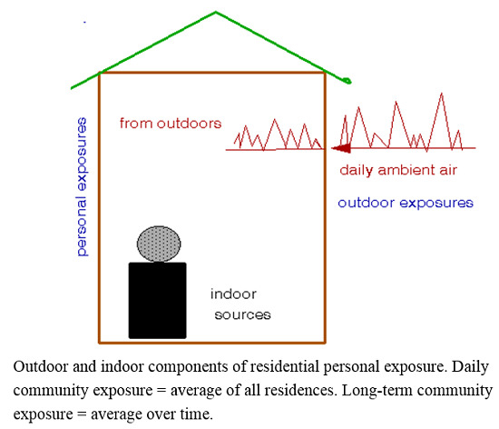
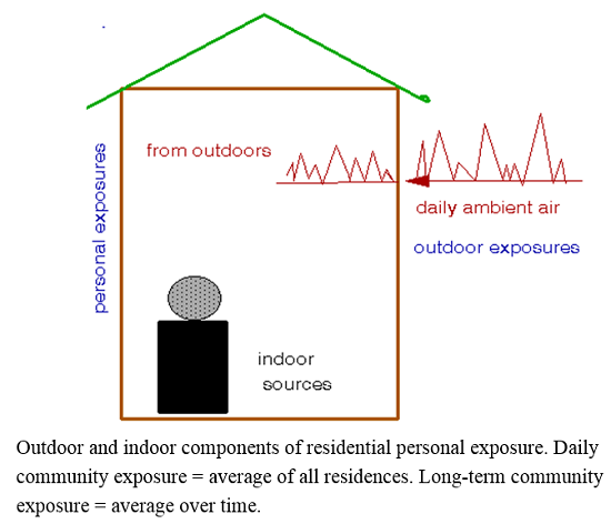
Developing appropriate exposure information for health effects studies is more complex and depends on the type of study. It is important to note that outdoor ambient air quality data may suffice to characterize the environment of a community but are unlikely to adequately characterize exposures of individuals within the community [1]. Further, exposures of only a few of those individuals are relevant to epidemiology. This conclusion has seldom been considered by epidemiologists in recent years. Other important considerations include:

• Regulatory standards may be based on studies that used incomplete exposure information [2].
• A complete description of community environment should include both indoor and outdoor conditions [3].

The paper is organized as follows: This section describes the rationale for the study and lays out the requirements for different types of exposure data. Section 2 describes the assessment methodology. In Section 3, I describe the exposure data I found in the literature and their characteristics. Section 4 then uses these data to estimate how different types of epidemiological studies would be affected by uncertainties inherent in the available exposure data and by the use of estimated personal exposures rather than the usual ambient air quality data. I discuss the implications of these findings in Section 5 and the resulting conclusions in Section 6.

1.1. Data Requirements by Type of Study

Studies involving controlled exposures of defined individuals require accurate and precise measurements of the pollutants involved; surrogate measures are unlikely to suffice [4]. By contrast, epidemiological methods are required to study populations large enough to detect the subtle health effects found under current conditions [5]. The often quoted aphorism, the dose makes the poison, applies here and requires considering each of element connecting ambient air quality to dose. The main elements are:

• Selection of pollutants to be considered
• Accuracy of measurement methods
• Spatial and temporal variability of outdoor air quality
• Penetration of outdoor air into occupied spaces
• Strengths of indoor pollution sources.

Other elements of uncertainty include indoor ventilation rates, rates of human uptake, and doses to target organs, for all of which adequate data are lacking.

Each of these elements involve uncertainties and requires averaging over populations; both regulated ambient (i.e., “criteria”) and toxic pollutants should be considered. Assessment requires comparing the relative contributions of each element of uncertainty with respect to the uncertainty in total exposure. For example, it would not be cost-effective to require a measurement method to have an accuracy of say, ±1%, if the uncertainty of the community average is say, ±10%. Similarly, if most exposures occur indoors, the accuracy of outdoor air measurements becomes less important for health studies. As outdoor air becomes cleaner, indoor pollution sources become more important. The processes linking exposure to target organ dose are perhaps the most problematic but have seldom been considered.

Reasons for neglecting personal exposures in air pollution epidemiology include:

• Regulatory mandates are limited to outdoor air [6].
• Indoor exposure information is not available for populations.
• Physiological processes governing doses to target organs are not well understood [7].
• Current epidemiological methods based on outdoor air quality have produced consistent and highly statistically significant findings that have been interpreted as individual risks [8].

Conventional epidemiological studies require parallel data on each parameter for all subjects, typically numbering in the thousands. With these deterministic methods, significance levels are largely determined by model fit. Typically, individual exposures are inferred from air quality data from a limited number of fixed ambient monitoring stations; the resulting uncertainties have been assessed in a number of studies. However, personal exposure data must be obtained on an individual basis and probabilistic methods are thus required to estimate population exposures. Survey sample sizes and the properties of exposure distributions will also affect significance levels of population-based risk estimates. The difficulties of this task do not diminish its relevance.

1.2. Exposure Data Requirements for Epidemiological Studies

Studies of population health fall into two categories: variations over time at selected locations (time-series studies) and variations among locations during selected time periods (cross-sectional studies). Although there may be some overlap, their respective data requirements differ substantially.

1.2.1. Time-Series Studies

Short-term (daily) variations are mainly driven by changes in weather such as stagnations, storms, or frontal passages. In such cases, ambient concentrations of various pollutants tend to show similar patterns. Shorter term (hourly) variations are largely due to occupational patterns or emission cycles such as vehicular traffic. Longer term cycles are usually seasonal, driven by both emissions and weather. A valid time-series study must control all of these patterns that relate to short-term health effects like mortality or hospitalization. Nevertheless, time-series studies have important advantages. They have been validated by major episodes of the past century during which excess daily death rates were high enough to allow identification of individual victims. They are not confounded by indoor pollution sources that remain largely unaffected by daily weather changes. However, only a fraction of outdoor air (typically ~ 50% [9]) penetrates indoors, thus attenuating actual exposures. Indoor/outdoor relationships must be averaged over the communities under study, which reduces the variance of these perturbations but not biases resulting from partial penetration of outdoor air.

The appropriate duration of exposure has not been established for epidemiological studies; statistical significance is often seen for multi-day periods [10]. Daily means are generally more relevant than hourly means for population-based studies because penetration of outdoor air is not instantaneous and the timing of peak hourly concentrations will vary within a population.

1.2.2. Cross-Sectional Studies

Longer term, usually annual, studies involve differences among communities and cohorts and must control for all other spatial differences that may relate to air quality. Since disadvantaged areas often have the worst air quality within a city, confounding may result from intercommunity differences in smoking, poverty, or education, all of which are known to exert larger effects on public health than air pollution [11]. Such differences can be difficult to control because of the multitude of such factors and lack of adequate data. In contrast with time-series studies, cross-sectional studies have not been validated by identifying specific putative victims Other issues involve timing and duration of exposures, including contributions of short-term exposures and allowance for the lag and latency for development of new diseases, for which cumulative exposures may be appropriate [12]. Persistent exposures from indoor pollution sources must also be considered and averaged across each community in the study. Exfiltration (venting of indoor air) is also possible and relates to the degree of building tightness, but adequate data are not available. However, forced ventilation may result in additional intake of outside air in order to maintain equilibrium.

Longitudinal studies [13] of gradual changes in exposures, of which few have been published, must control for other long-term changes including improved medical care, better residential construction, and reduced rates of smoking.

1.2.3. Summary

Sources of exposure uncertainty in epidemiology include:

For time-series studies, sources include instrument accuracy and spatial variation of daily outdoor air quality averaged over the number of monitoring locations and annual rate of infiltration of outdoor air averaged over the number of residences in the community under study. Seasonal variations in infiltration rates might also be considered.

For cross-sectional studies, sources include instrument accuracy and annual spatial variation of outdoor air quality averaged over the number of monitoring locations in each city, infiltration of outdoor air averaged over the number of residences in each city, and annual average contributions of indoor sources averaged over the number of residences in each city.

Each of these parameters will vary by pollutant, and it is likely that outdoor and indoor air quality may involve different species. Although this paper emphasizes particles, pollutants of interest should not be limited to criteria pollutants but should include toxic species of known health effects, especially those found indoors.

2. Methods and Data

The basic method of assessment involves postulating baseline datasets and hypothetical linear regressions of mortality on pollution, as if the mortality rates were adjusted for confounding variables. These regressions are then repeated using exposure data modified to reflect outdoor air quality variability, penetration into residences, and indoor air pollution sources, sequentially. The data required to estimate these exposure variations were obtained from the literature and expressed as exposure increments and their standard errors. The outcome of the assessment is the degree to which regression coefficients and their standard errors differ from baseline values according to definitions of exposure.

3. Results

Data are available for each of these exposure parameters for several pollutants; fine particulate matter (PM_2.5) was selected as an illustrative example. Personal exposures are often assumed to be tantamount to indoor concentrations, which comprise infiltrated outdoor air and emissions from indoor sources [14]. However, indoor air quality relates to the average personal exposures of all the individuals in the household during the study period and is thus less difficult to model.

Indoor sources comprise key constituents of personal exposure for all types of health studies including toxicological studies of sick building syndrome and the like [15]. An epidemiology study based only on outdoor air quality, as has been the case, tacitly assumes that indoor sources may be neglected, ostensibly because they are not regulated under the Clean Air Act. As shown below, this assumption has important implications for epidemiology and estimates of health effects

3.1. Outdoor Air Concentrations

Many studies of daily variations in health parameters have been based on a few or single air quality monitoring stations; spatial and/or temporal air quality variability could thus be an important contributor to uncertainties in health effect estimates. Uncertainties in outdoor air concentrations, including spatial variability and instrumental or analytical precision, reflect directly on personal exposures to outdoor air.

The daily PM_2.5 data of Pinto et al. [16] for 27 urban areas that had multiple monitors for the year 2000 appear to be the best dataset for studying intracity spatial variations. Pinto et al. list the ranges in inter site means and site-pair correlations as indices of spatial variability. The correlations between pairs indicate their consistency over time irrespective of mean values, which is important for time-series studies. The ranges of mean values indicate variability for use in long-term studies. Neither of these statistics provides direct estimates of spatial uncertainties in outdoor air quality for comparison with those for indoor air quality, which are estimated as follows.

The definition of the correlation coefficient R is useful in this regard:

R² = 1−σ_xy²/σ_y²

(1)

where σ_xy² is the unexplained variance from a linear regression of y on x, which in this case are parallel records of daily PM_2.5 in a given city, and σ_y is the corresponding standard deviation. Unfortunately, σ_y values are not tabulated by Pinto et al. so that estimation is required from other sources. For this purpose, PM₁₀ data was drawn upon for the 20 largest USA cities [17] and estimated a standard deviation for each city using the tabulated means and 10th and 90th percentiles. Note that PM₁₀ and PM_2.5 have the same coefficients of variation (0.29) across cities [18] and thus similar frequency distributions. 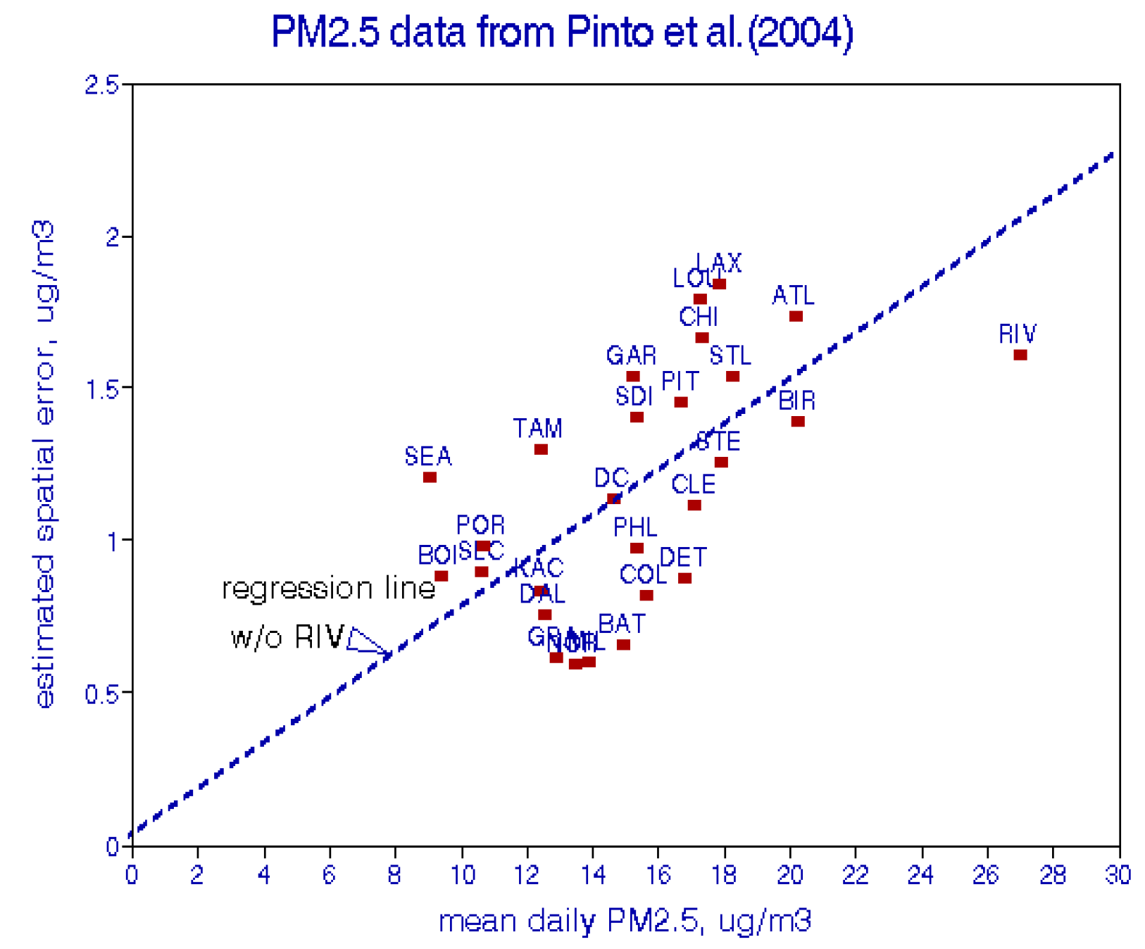The ratios of estimated deviation to mean PM₁₀ ranged from 0.20 to 0.43 with a mean of 0.30 and a standard deviation of 0.56. These estimates are considered adequate for the purposes of comparative analyses in this paper and used a mean value of 0.3 to estimate σ_y. Equation (1) was then used to estimate σ_xy for each city as shown in Figure 1.

Figure 1. Estimated spatial PM_2.5 uncertainties for 27 USA cities [16].

Figure 1. Estimated spatial PM_2.5 uncertainties for 27 USA cities [16].

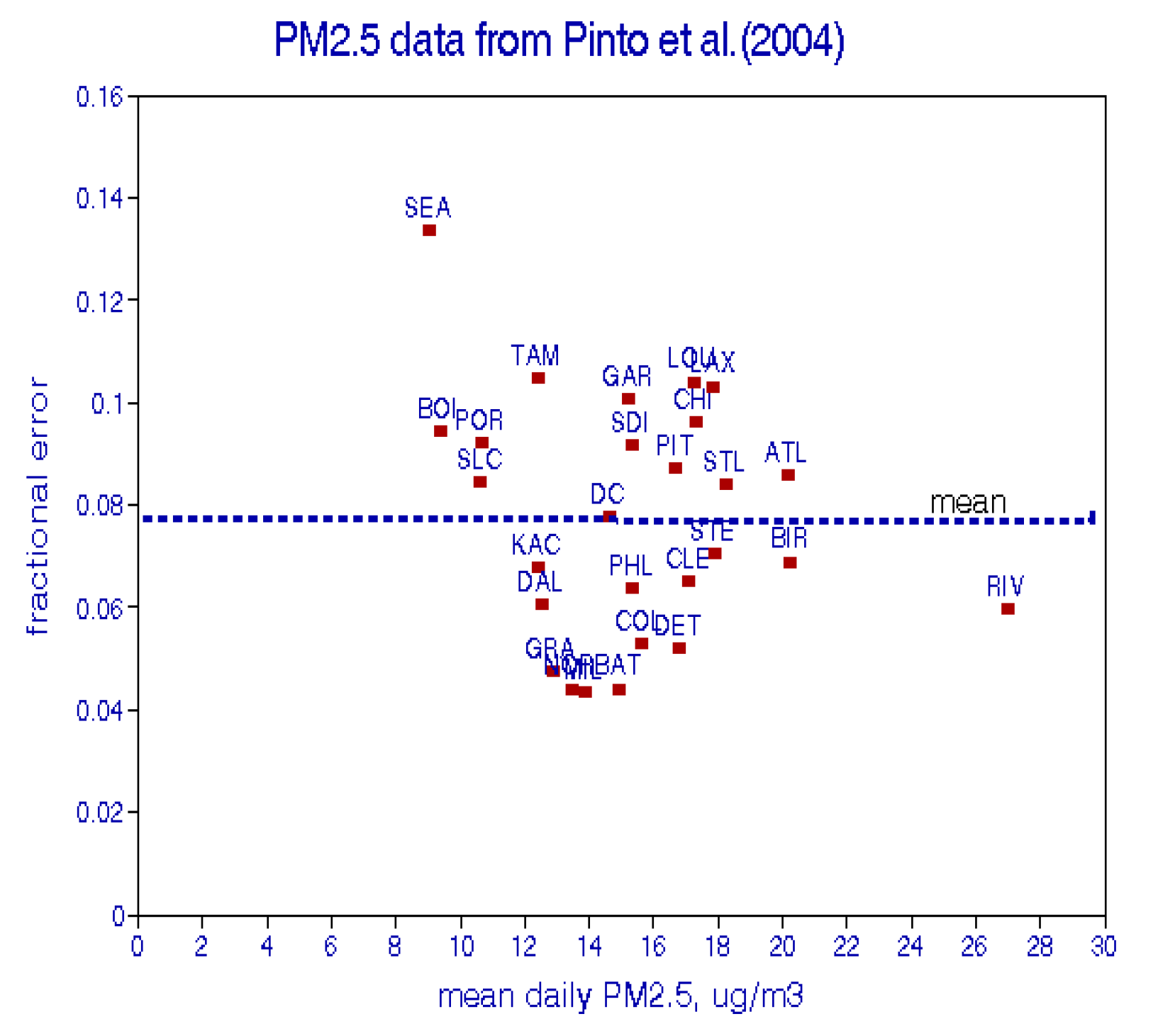
Figure 2. Fractional spatial uncertainties for 27 USA cities [16].

Figure 2. Fractional spatial uncertainties for 27 USA cities [16].

These estimated errors are highly correlated with mean PM_2.5 with an average ratio of error to mean of 0.077 (Figure 2). At 15 μg/m³, the 95% confidence intervals for a single monitoring station would thus be (12.7, 17.3). For the average over a network of 10 stations, the CIs would be (14.6, 15.4). As discussed below, corresponding indoor values for infiltrated outside air would be approximately half of these estimates. Note that the averaging process for outdoor air pertains to the number of monitoring stations within a city, while averaging for indoor air pertains to the number of households in that city.

3.2. Infiltration of Outdoor Air

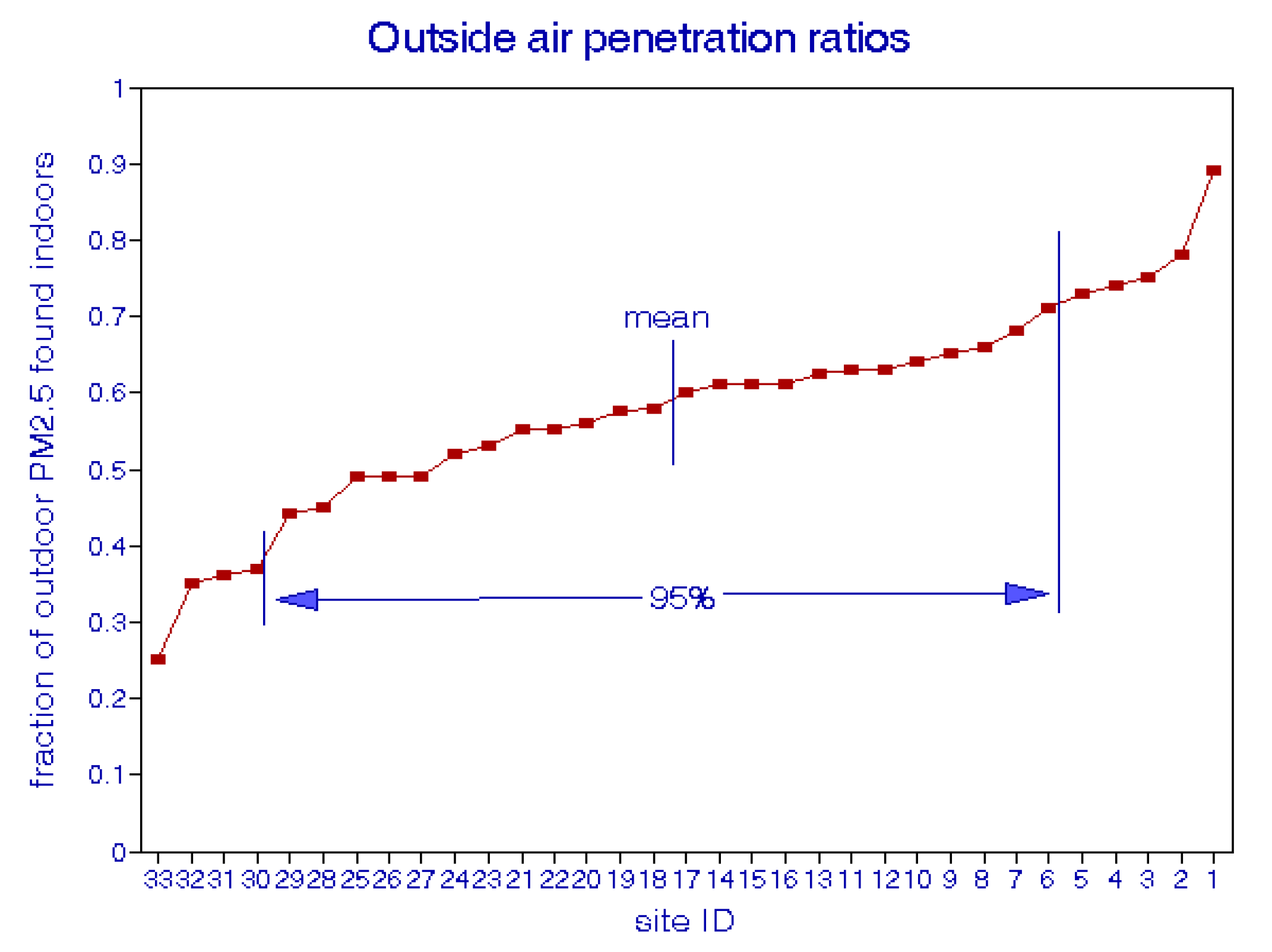
Infiltration has been studied extensively in USA and abroad. A good approximation of the mean rate is about 0.50 and a typical distribution is shown in Figure 3; the standard deviation is about 0.07 [9]. However, epidemiology studies involve large populations and community averages over thousands of residences. The variability among individual buildings is thus of little importance, assuming minimal seasonal variations or correlations with other community attributes like income, education, proximity to pollution sources like traffic. Nevertheless, accounting for infiltration has the effect of doubling risk estimates because only half of the outdoor concentration could be responsible for health effects observed indoors.

Figure 3. Distribution of outdoor air penetration ratios for individual buildings [9].

Figure 3. Distribution of outdoor air penetration ratios for individual buildings [9].

3.3. Indoor Air Pollution Sources

Many studies have characterized specific types of indoor particulate air pollution such as environmental tobacco smoke (ETS), pet dander, indoor combustion source including gas stoves, candles, incense, household dust [15]. Note that current regulatory practice considers the mass but not the chemistry of PM. In the developed world, the most common indoor pollutants are NO₂, CO, and particulate matter, especially PM_2.5. Aside from photocopy machines, there are no indoor sources of O₃, and SO₂ tends to be adsorbed onto interior surfaces. Important indoor non-criteria pollutants include NH₃, benzene, and formaldehyde, all of which are known to cause adverse health effects [19]. Acid aerosols tend to be neutralized indoors [20]. It is quite possible that important indoor pollutants may differ from outdoor species, requiring consideration of mixtures.

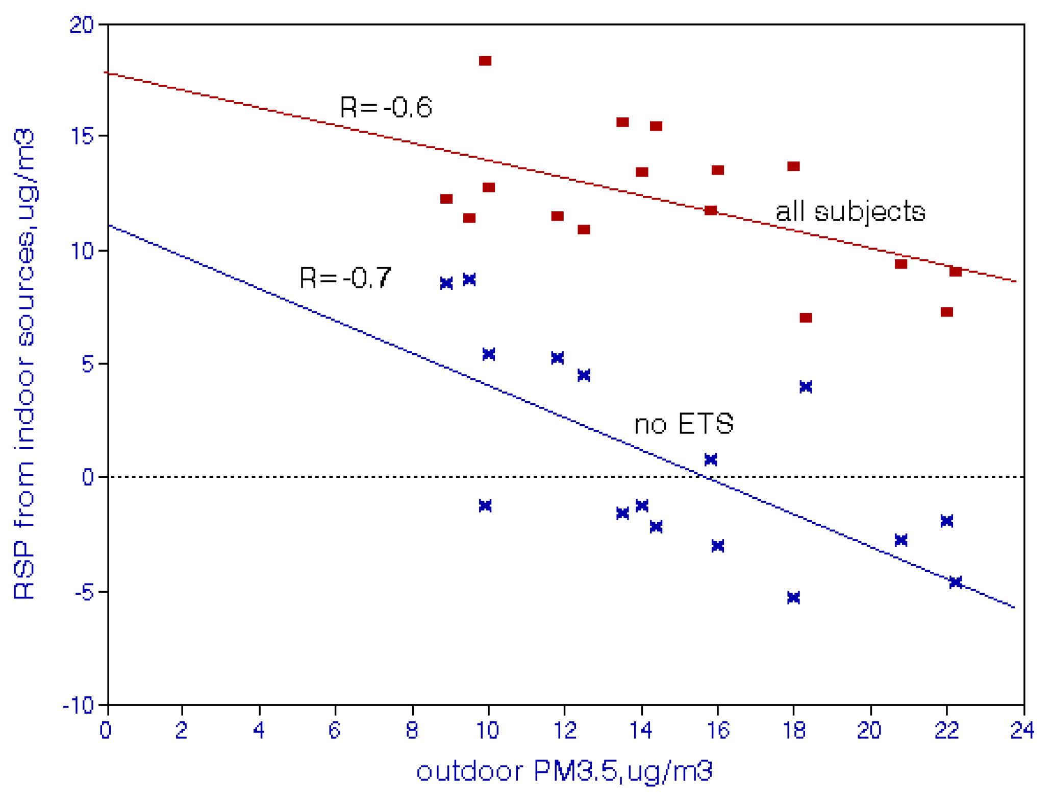
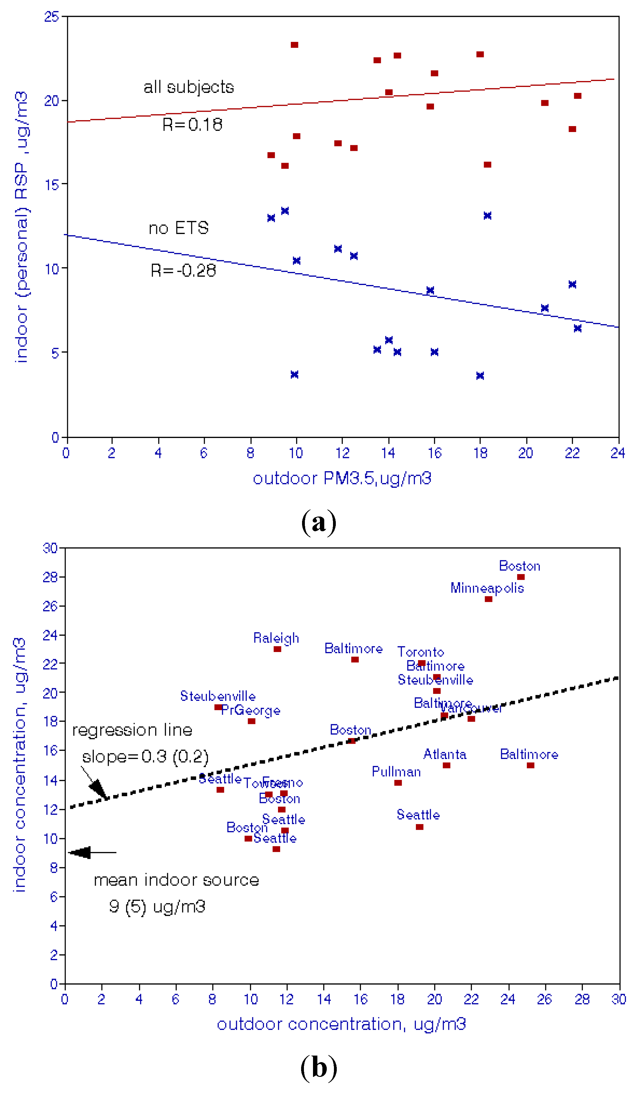
ETS may be the most important source of indoor PM_2.5. Jenkins et al. [21] measured personal exposures to respirable particulates (RSP, PM_3.5)* for 100 nonsmokers in each of 16 metropolitan areas and contrasted the results according to passive smoking in their work and home environments. The results are shown in Figure 4, with an RSP range of 8–15 μg/m³ due to ETS. There is also a negative relationship with outdoor levels. Spengler et al. [22] reported an indoor RSP increment of 20 μg/m³ when two smokers were present, which is consistent with Figure 4.

Figure 4. Effects of environmental tobacco smoke on indoor PM_3.5 concentrations in 16 USA cities [21]. In the 1980s, fine particles were designated “respirable particles” (RSP), defined as PM_3.5.

Figure 4. Effects of environmental tobacco smoke on indoor PM_3.5 concentrations in 16 USA cities [21]. In the 1980s, fine particles were designated “respirable particles” (RSP), defined as PM_3.5.

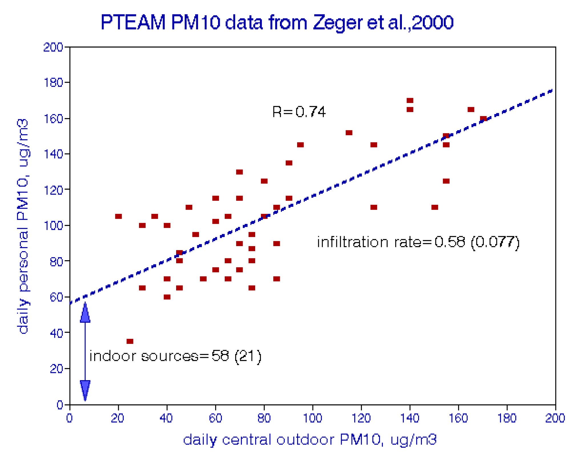
The contributions of indoor sources cannot be measured directly but may be inferred by regressing indoor concentrations on outdoor levels. The time-series data of Zeger et al. [23] for Riverside, CA shown in Figure 5 are useful for this purpose. The slope (0.58) represents the infiltration rate of outdoor air while the intercept (58 μg/m³) represents contributions of indoor sources. Both of these estimates are highly statistically significant. 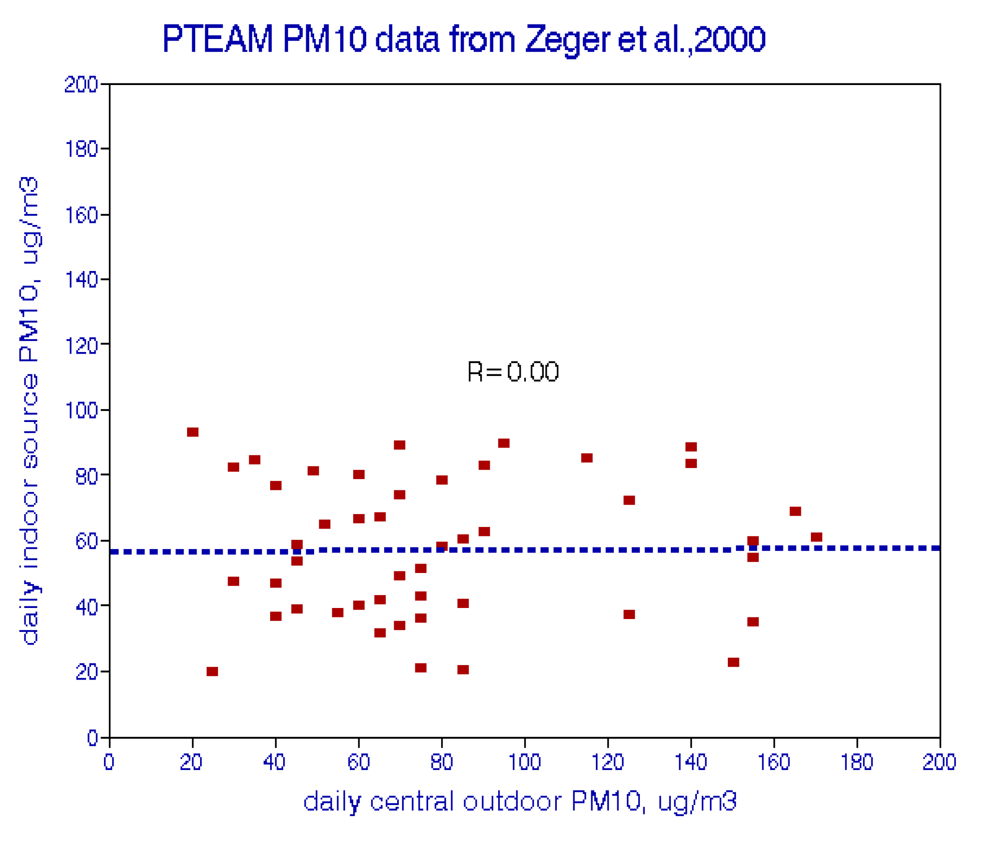Figure 6 implies that the effects of indoor sources do not vary over time at this location.

Figure 5. Indoor/outdoor PM₁₀ relationships from Riverside, CA [23].

Figure 5. Indoor/outdoor PM₁₀ relationships from Riverside, CA [23].

Figure 6. Estimated effects of indoor PM₁₀ sources in Riverside, CA [23].

Figure 6. Estimated effects of indoor PM₁₀ sources in Riverside, CA [23].

Figure 7. Indoor-outdoor PM_2.5 relationships among USA: (a) Cities [21]; (b) Cities [24] Note: ( ) denotes standard error.

Figure 7. Indoor-outdoor PM_2.5 relationships among USA: (a) Cities [21]; (b) Cities [24] Note: ( ) denotes standard error.

.

Mean particulate levels tend to vary more between cities than within a city, especially for fine particles. Jenkins et al. [20] sampled outdoor and indoor respirable particulates in 16 US cities; Avery et al. [23] present detailed PM_2.5 sampling data from 34 USA cities. The contributions of indoor sources were estimated by subtracting 50% of the outdoor concentration from the indoor concentration. Caution is in order here because the small samples in each city may not adequately represent city-wide averages. These results are shown in Figure 7a,b which show that personal exposures cannot be predicted from outdoor concentration levels. The mean indoor source contribution from Avery et al. [24] is 9 μg/m³; from Jenkins et al. [21], 12 μg/m³ for all subjects and 0.9 μg/m³ in the absence of ETS. Thus, with respect to cross-sectional analysis, mean ambient concentration is a poor surrogate for actual (personal) exposure, even in nonsmoking households, even though they may be correlated over time in each city.

Adverse effects of ETS have been reported in epidemiological studies [25,26]. However, I found no air pollution studies that accounted for ETS increments to PM exposures. “Control” for passive smoking in regression analysis does not meet this requirement. In this regard, “% smokers” is probably a more appropriate confounding variable than “yes/no” for individual primary smokers.

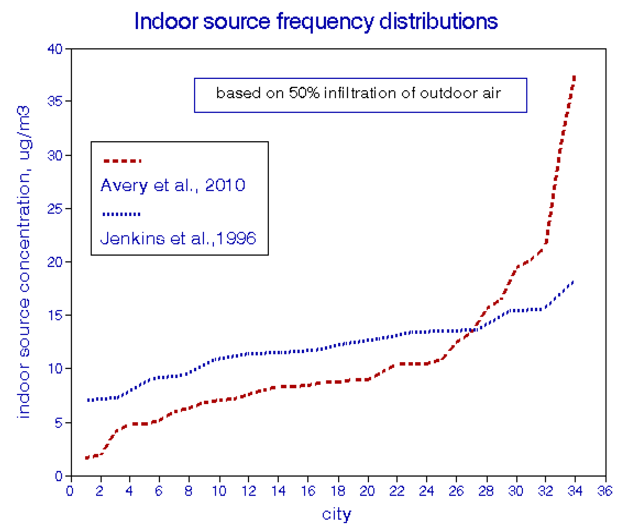
Frequency distributions of these two sets of multi-city data are shown in Figure 8. The distribution of data from Jenkins et al. [21] is well behaved, in contrast to the data from Avery et al. [24], for which about 7% of cities had lower concentrations than expected and about 25% were higher. The remaining two-thirds of the cities had indoor source contributions in the expected range of 5–10 μg/m³. Specific reasons for the different distributions in these two studies are unknown and may comprise further sources of uncertainty.

Figure 8. Estimated frequency distributions of city-average PM_2.5 concentrations from indoor sources [21,24].

Figure 8. Estimated frequency distributions of city-average PM_2.5 concentrations from indoor sources [21,24].

4. Simulated Epidemiological Analyses

To illustrate potential effects of exposure uncertainties on epidemiological exposure-response relationships, a time-series of 1000 days and regressed simulated daily mortality variables against alternative exposure variables was simulated. Similar cross-sectional regressions for a cross-sectional dataset for 100 cities were ran. In the time-series analysis, the “true” PM_2.5 concentration was set at 15 μg/m³ for all days, as if seasonal and temperature effects had been removed. Random effects of spatial variability of outdoor air and the penetration to the indoors were simulated; indoor sources were assumed to be invariant on a daily basis and were not considered. Since these simulated series have no serial correlation, lag effects could not be considered.

The cross-sectional analysis included spatial variability of outdoor air and indoor penetration and parametric effects of arbitrary indoor sources. Mean PM₁₀ values for 20 large cities [17] were used to establish the baseline distributions; PM_2.5 was then assumed to be about half of PM₁₀ on average [9] and the dataset was replicated five times in order to provide an arbitrary set of 100 cities. The sources of variability included the spatial data of Pinto et al. [16], a mean infiltration rate of 0.5, and the indoor source distributions of either Avery et al. [24] or Jenkins et al. [21]. The analysis assumed that indoor source strengths are independent of outdoor air quality, as shown in the figures above.

The mean mortality rate was set at 35 deaths/day and the baseline PM_2.5 regression coefficient at 0.25. Random errors at various levels using a spread-sheet random function were introduced and found that 10 regression replications provided adequate numerical stability as judged by the similarity of the standard deviation across replications with respect to the average of the standard errors of each of the 10 regressions. Both analyses assume that the mortality variables have been adjusted for all confounders, such that pollution exposure is the only independent variable. These simulations are intended to serve as examples of what personal exposures might be expected, rather than precise estimates of actual situations. Table 1 provides summary statistics for the variables used in these simulations.

Table 1. Statistics of variables used in simulations

			Mean	Std. dev.	CV
A. Simulated time-series analyses	base PM2.5 with instrument error	15		0.89	0.059
	with infiltration error 1	7.5		0.48	0.064
	with additional error 2	7.5		0.53	0.071
	with additional error 2.5	7.5		0.59	0.079
	with additional error 3	7.5		0.61	0.081
	with additional error 4	7.5		0.8	0.106
	mortality	38.75		1.74	0.045
B. Simulated cross-sectional analyses	base PM2.5	16.5		3.25	0.2
	w/spatial error	19		3.65	0.19
	w/infiltration	9.5		1.82	0.19
	w/100% indoor sources	33.9		12.2	0.36
	w/50% indoor sources	22.1		6.87	0.31
	w/25% indoor sources	16.2		4.62	0.29
	w/15% indoor sources	13		2.68	0.21
	mortality	39.1		1.67	0.043

Table 1. Statistics of variables used in simulations

			Mean	Std. dev.	CV
A. Simulated time-series analyses	base PM2.5 with instrument error	15		0.89	0.059
	with infiltration error 1	7.5		0.48	0.064
	with additional error 2	7.5		0.53	0.071
	with additional error 2.5	7.5		0.59	0.079
	with additional error 3	7.5		0.61	0.081
	with additional error 4	7.5		0.8	0.106
	mortality	38.75		1.74	0.045
B. Simulated cross-sectional analyses	base PM2.5	16.5		3.25	0.2
	w/spatial error	19		3.65	0.19
	w/infiltration	9.5		1.82	0.19
	w/100% indoor sources	33.9		12.2	0.36
	w/50% indoor sources	22.1		6.87	0.31
	w/25% indoor sources	16.2		4.62	0.29
	w/15% indoor sources	13		2.68	0.21
	mortality	39.1		1.67	0.043

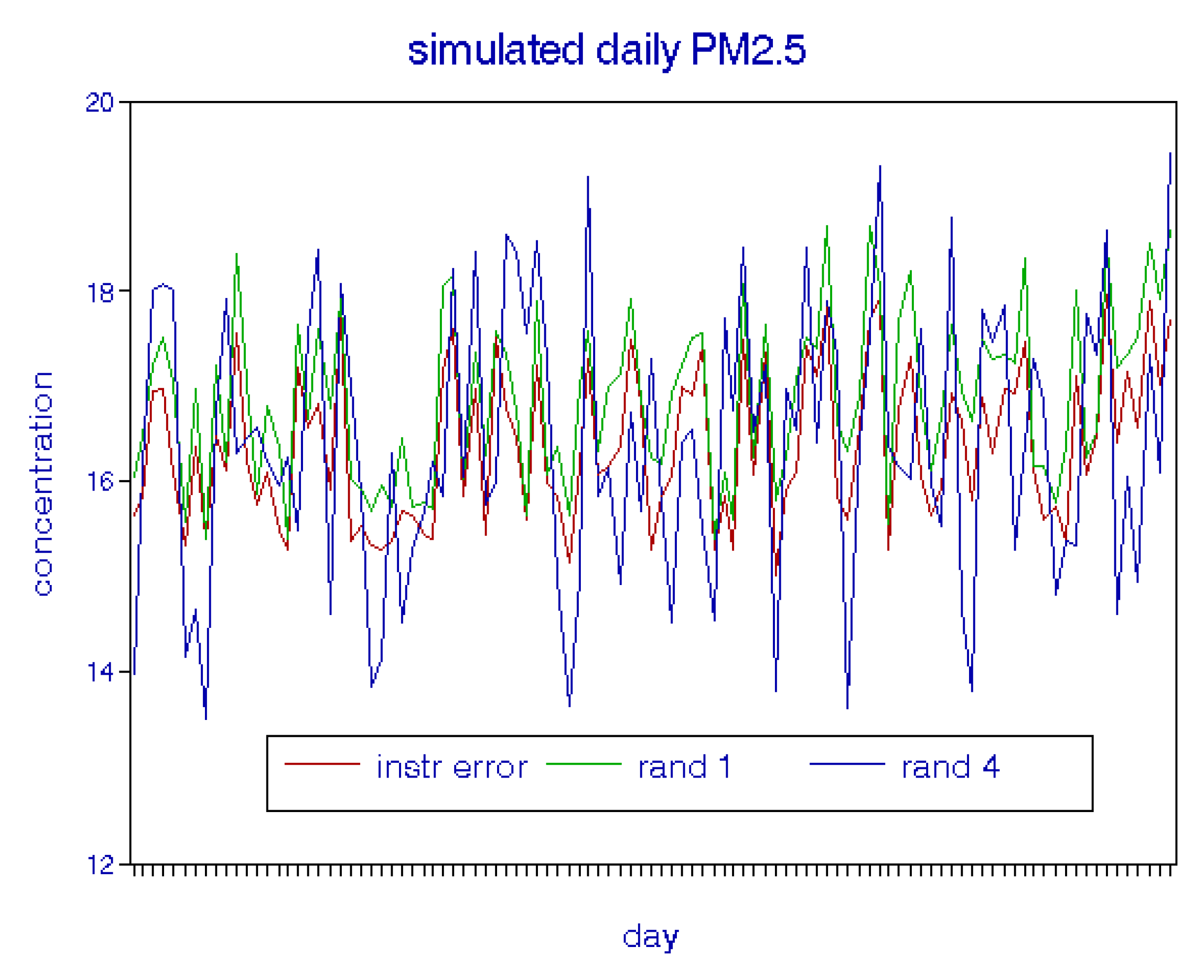
4.1. Time-Series Simulations

Figure 9 shows that, as spatial errors are added, the exposure sequences track well but regression coefficients are attenuated and tend to lose statistical significance. When infiltration to the indoors is considered, exposures are halved and thus regression coefficients are essentially doubled.

Figure 9. Sample of simulated daily variations in PM_2.5 with error added.

Figure 9. Sample of simulated daily variations in PM_2.5 with error added.

4.2. Cross-Sectional Simulations

I used the data of Pinto et al. [16] to estimate the spatial variability of outdoor PM_2.5 within each city. As seen in Figure 3, the mean fractional error in a given city is 7.7% with a standard deviation of 2.3%. This baseline distribution was then perturbed randomly among cities. The outdoor air infiltration rate was held constant at 0.5 for these simulations With respect to indoor pollution sources from Avery et al. [24], a quasi-normal distribution was able to be fit to Figure 8 by discarding the two lowest values and exponentiating the data to successively lower powers. The best fit was obtained using the 0.05 power of concentration, which produced a correlation coefficient of 0.95 and 95% confidence intervals of 1.5 and 46 μg/m³. For the data of Jenkins et al. [21], the distribution of indoor sources was assumed to be normal with a mean of 12.1 μg/m³ and standard deviation of 2.9.

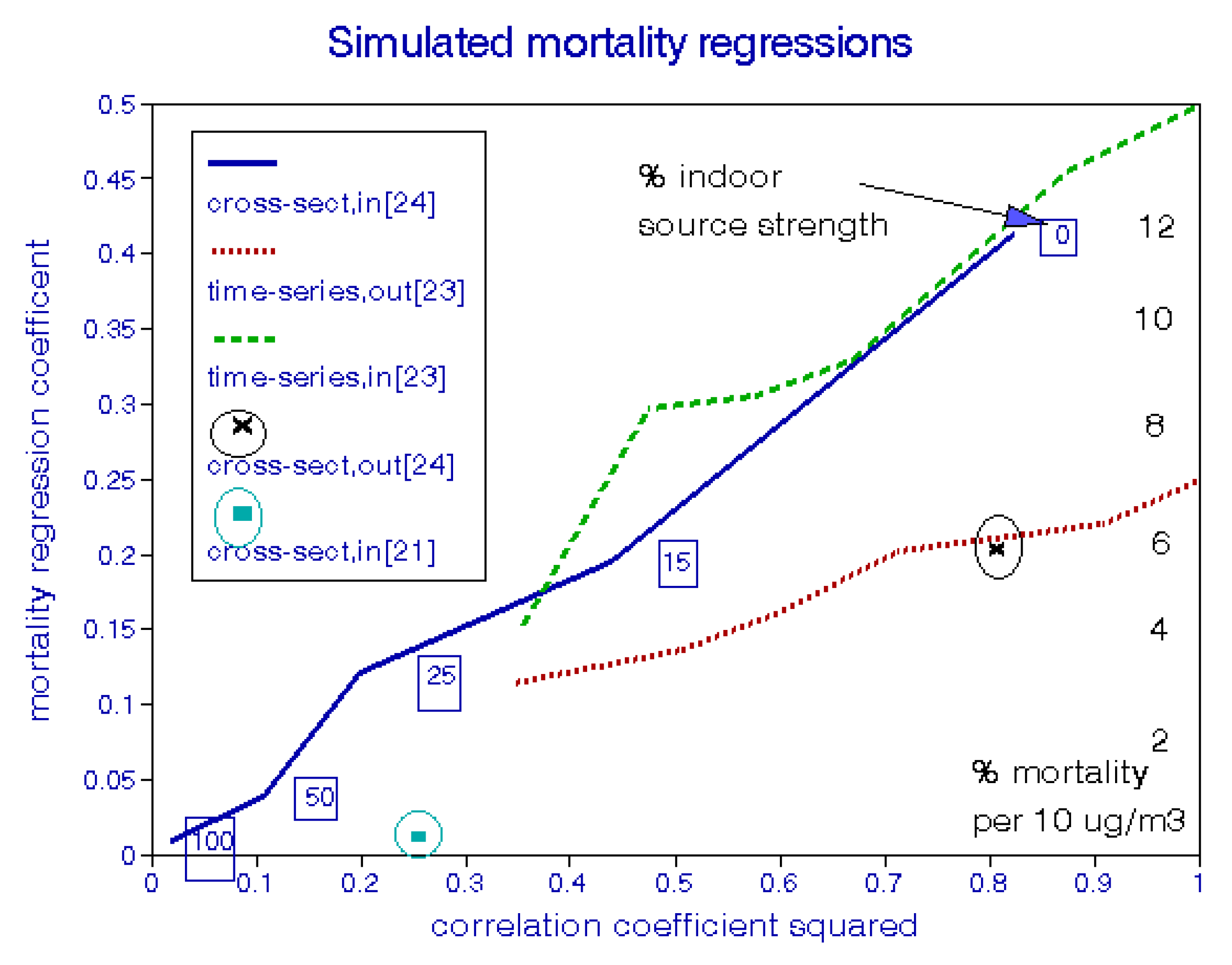
4.3. Simulation Results

Figure 10 compares the results of these time-series and cross-sectional simulations in response to reduced correlation between exposure variables. In the absence of error, the 50% infiltration rate has the effect of doubling either regression coefficient, as shown at the right of the figure. For convenience, the regression coefficient scale is also converted to percent mortality change per 10 μg/m³ (right-hand scale). Attenuation of the outdoor time-series coefficients results from increasing spatial errors; for example, correlations between daily data from monitors in the same city are frequently around 0.8, which results in a coefficient reduction of about 30%, without considering indoor air quality. However, these effects of outdoor variability are more than compensated for by the biasing effect of partial penetration to the indoors. Intra-city variations in infiltration are of little concern because they would be averaged over the number of residences in each city under study.

Figure 10. Simulated attenuation of regression coefficients by uncertain outdoor air quality, indoor infiltration, and indoor pollution sources.

Figure 10. Simulated attenuation of regression coefficients by uncertain outdoor air quality, indoor infiltration, and indoor pollution sources.

Only one data point is shown for the cross-sectional model with outdoor data, for which the attenuation is due to spatial variability. The baseline cross-sectional analysis involves a much larger range in exposures based on the original set of cities selected. As with the time-series simulations, regression coefficients are doubled because of the 50% indoor penetration rate [9]. However, they can be greatly attenuated by effects of indoor sources. The initial simulation is based on the indoor source distribution of Figure 8; with this level of pollution from indoor sources, the relationship between personal exposure and mortality becomes nil. As a result, fractions of this indoor source level were used in order to generate a range of coefficient attenuation for comparison. The mean concentration of infiltrated outdoor air is about 9.6 μg/m³ and adding 15% of the Avery et al. [24] indoor source contribution (3.4 μg/m³) attenuates the cross-sectional mortality regression by more than 50%, placing it well within the range of attenuated time-series regression coefficients.

Using the indoor source distribution based on the data of Jenkins et al. [21] reduced the simulated mortality regression coefficient to essentially zero, as is the case with the full-strength data from Avery et al. [24].

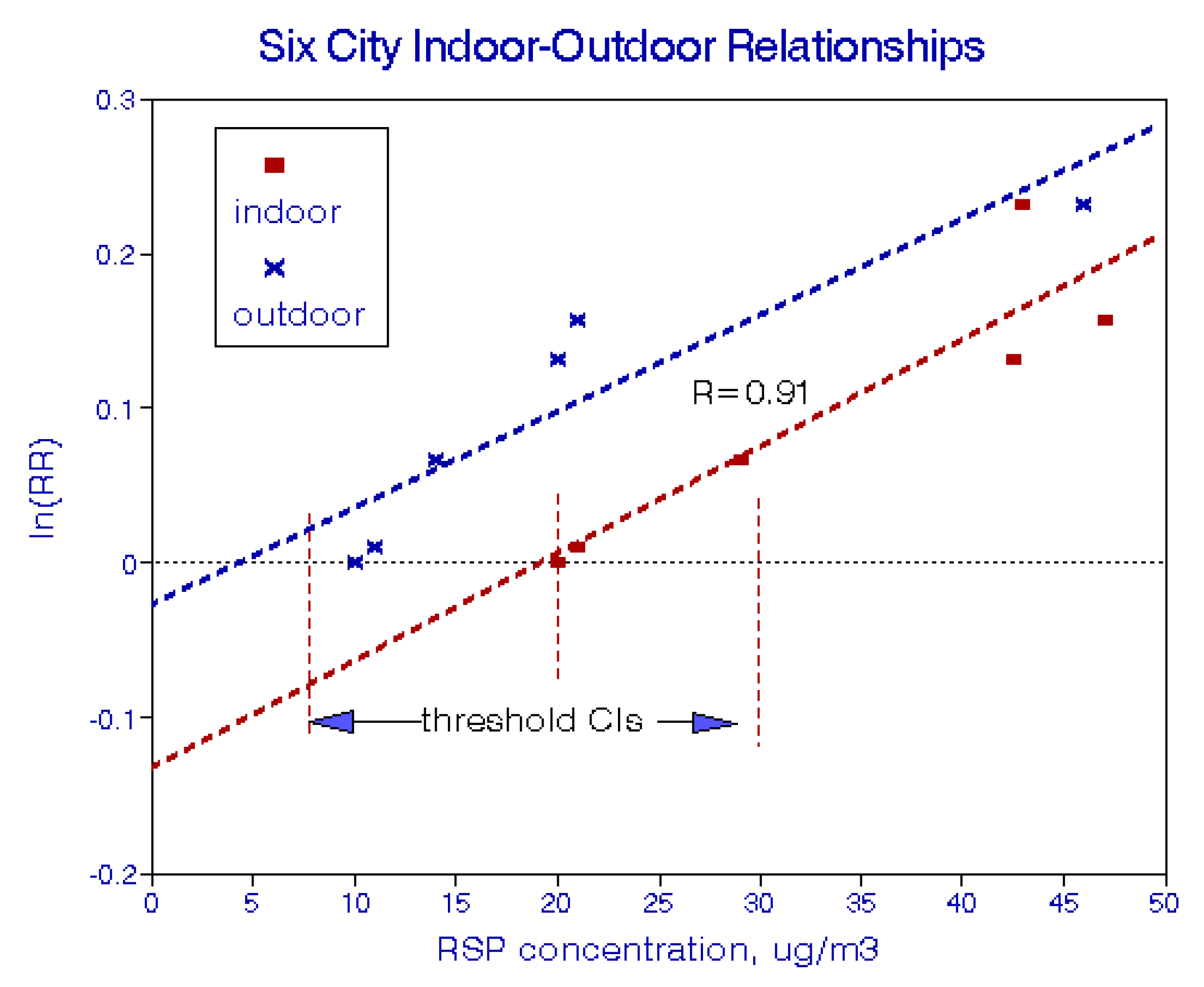
4.4. Attenuation with Actual Epidemiological Data

A further example of regression attenuation may be seen with data from the Harvard Six Cities Study. Spengler et al. [22] reported personal RSP exposures for each city, and Dockery et al. [27] reported relative mortality risks. These data are combined in Figure 11, based on either outdoor data or personal exposures. The two exposure-response lines are roughly parallel, but using the higher personal exposures shifts the dose-response function to the right, implying a statistically significant threshold of about 20 μg/m³.

Figure 11. Exposure-response relationships from the Harvard Six Cities Study.

Figure 11. Exposure-response relationships from the Harvard Six Cities Study.

5. Implications

Uncertainties in exposure to air pollution have long been known to epidemiologists but seldom explored in detail, with the possible exception of spatial variability in outdoor concentrations. Most epidemiology studies use averages over the relevant ambient monitoring stations in a given city, but such spatial variability can be important when only a few monitoring sites are available in a given city. In time-series studies of daily events, data from nearby monitoring sites may be highly correlated, depending on the pollutant, but there are also issues of bias due to variability in mean values. These issues are relevant to most epidemiology studies.

However, variability in outdoor air quality comprises only a minor portion of the combined uncertainties in total (personal) exposures, which include variable rates of infiltration of outdoor air into occupied spaces and effects of many different indoor sources of air pollution. Infiltration is a factor for all types of epidemiology studies and these rates are well defined. Effects of indoor sources generally relate only to long-term studies, including cohort studies. This distinction creates a hierarchy in epidemiology studies, with daily time-series being the least affected and cross-sectional studies the most affected.

Figure 10 shows that time-series studies of 1000 days and cross-sectional studies of 100 cities will have equivalent regression attenuation for a given exposure uncertainty, but that cross-sectional studies are inherently less reliable since they are subject to additional uncertainties from indoor pollution sources.

In terms of optimizing exposure information for epidemiology, the most critical data needs relate to distributions of indoor pollution sources within and between cities. Because of averaging within cities, the accuracy for any one building may be less important than the number of cities with at least some rudimentary data; i.e., in this sense, quantity may be more important than quality.

Figure 7 shows that indoor air quality is essentially unrelated to outdoor air quality across cities. Interpretation of all the extant cross-sectional studies, including cohort studies, is thus in question. Since such studies have played a large part in setting ambient air quality standards, this finding could have important regulatory implications.

Studying the health effects of indoor sources could be quite data intensive, requiring linkage between individual decedents and their residential characteristics. Privacy concerns may well preclude such an investigation. Nevertheless, the public should be aware of the risks of indoor air about which they have some control as well as the community levels of outdoor air quality subject to regulation.

6. Conclusions

Measured outdoor air quality is subject to uncertainties due to monitoring site location and analytical errors. Intersite variability in mean PM_2.5 showed a mean standard error of 7.7% among 27 USA cities, so that 95% confidence intervals would be (12.7–17.3) μg/m³ for a single monitoring station at 15 μg/m³. Multi-site data are thus strongly preferred for epidemiological studies and regulatory decisions.

Personal exposure is tantamount to indoor concentration for epidemiological purposes. Indoor air pollution emanates from infiltrated outdoor air and emissions from indoor sources. Rates of infiltration average about 50%, are reasonably well-defined, and contribute little uncertainty to exposure averaged across a city because of strong correlations between ambient and infiltrated outdoor concentrations. However, the decrease in mean effective exposure biases regression coefficients based on outdoor air such that the true effects of time-dependent exposures may be up to twice those of current estimates. Slowly varying indoor sources have essentially no effect on time-series analyses although base concentration levels would be affected.

By contrast, intercity variations in the mean contributions of indoor sources can strongly affect cross-sectional studies. Two independent studies of groups of USA cities show no correlation between mean indoor and outdoor concentrations. As a result, effect estimates from long-term cross-sectional and cohort studies may have been over-estimated. The largest contributions to indoor air pollution are from environmental tobacco smoke; contributions from other indoor pollution sources also vary widely among cities but have little effect when averaged across a group of cities.

All of these findings are based on small samples of indoor air and rudimentary Monte-Carlo analyses. Larger samples of indoor air quality are needed across many more cities for various criteria and non-criteria pollutants including PM size and composition, after which full-fledged probabilistic analyses would be appropriate for various health endpoints. Pending such verification, comparisons between time-series and cross-sectional studies remain problematic as does use of the latter for regulation.