Spatiotemporal Interpolation of Rainfall by Combining BME Theory and Satellite Rainfall Estimates

Abstract

The accurate assessment of spatiotemporal rainfall variability is a crucial and challenging task in many hydrological applications, mainly due to the lack of a sufficient number of rain gauges. The purpose of the present study is to investigate the spatiotemporal variations of annual and monthly rainfall over Fujian province in China by combining the Bayesian maximum entropy (BME) method and satellite rainfall estimates. Specifically, based on annual and monthly rainfall data at 20 meteorological stations from 2000 to 2012, (1) the BME method with Tropical Rainfall Measuring Mission (TRMM) estimates considered as soft data, (2) ordinary kriging (OK) and (3) cokriging (CK) were employed to model the spatiotemporal variations of rainfall in Fujian province. Subsequently, the performance of these methods was evaluated using cross-validation statistics. The results demonstrated that BME with TRMM as soft data (BME-TRMM) performed better than the other two methods, generating rainfall maps that represented the local rainfall disparities in a more realistic manner. Of the three interpolation (mapping) methods, the mean absolute error (MAE) and root mean square error (RMSE) values of the BME-TRMM method were the smallest. In conclusion, the BME-TRMM method improved spatiotemporal rainfall modeling and mapping by integrating hard data and soft information. Lastly, the study identified new opportunities concerning the application of TRMM rainfall estimates.

1. Introduction

Rainfall is often one of the most important input parameters in hydrological modeling [1]. Highly accurate estimation of the spatiotemporal rainfall distribution over a geographical region is a crucial component of many scientific studies, such as soil erosion research, disaster forecasting, ecological and environmental management. However, obtaining accurate rainfall data remains a challenging affair mainly due to the lack of a sufficient number of rain gauges in mountainous areas and the inconsistent spatial distribution of rain gauges over different parts of watersheds.

An alternative and reliable method for acquiring rainfall data is spatial interpolation. In recent years, various conventional interpolation methods, such as Thiessen polygon and inverse distance weighted (IDW) [2,3] and geostatistical methods (including different types of kriging and cokriging techniques), have been widely used to produce areal rainfall estimates from point measurements. A number of studies have compared conventional and geostatistical methods by means of cross-validation statistics, and they found that kriging is among the best methods available [4,5,6]. However, geostatistical methods, such as kriging, rather apply formal techniques of pattern fitting (regression analysis, sampling theory, etc.) and do not consider in situ uncertainties and diverse site-specific information sources in a systematic manner [7]. On the other hand, the Bayesian maximum entropy (BME) [8,9] rigorously incorporates the existing dataset uncertainty and provides a mathematical framework for assimilating a wide variety of information sources that are beyond the scope of mainstream kriging methods [10,11]. In particular, BME overcomes many shortcomings of conventional interpolation methods: BME is a nonlinear interpolation method [12,13,14]; it allows for non-Gaussian distributions, in general [15]; and it provides the complete probability law at each space-time point rather than a single estimate [16,17]. Furthermore, BME can assimilate a variety of relevant information sources, by classifying them into a core knowledge base (general (G)-KB; which may include physical laws, primitive equations and theoretical models of space-time dependence) and a site-specific knowledge base (S-KB; including hard data obtained across the site, i.e., measurements that can be considered exact for all practical purposes, as well as soft information, i.e., data with fair or considerable degrees of uncertainty) [18]. BME’s potential to achieve better performance than other methods is mainly due to noticeable progress in its application range, covering an increasing number of fields, including spatial prediction of soil properties [19,20], urban climate research [12], marine geodesy [21], water quality assessment [22], fecal pollution and rainfall patterns [23], spatiotemporal ozone distribution [24,25], fine particulate matter pollution [26], disease risk analysis [27] and the study of epidemic spread [28,29].

Real-world case studies that compared BME and kriging have found that the maps generated using BME are more accurate and reliable than those produced by kriging [20,30]. In Yang et al. [31], BME performed better than both ordinary kriging and regression kriging in the prediction of soil organic matter content. The results obtained by Akita et al. [32] and by Messier et al. [33] showed that BME’s assimilation of secondary information can significantly improve prediction accuracy. These results do not come as a surprise, since, in theory, kriging is a special case of BME under limiting conditions [10]. As a result, BME must perform at least as good as, say, ordinary kriging, in the limiting case that linear estimators and Gaussian distributions are considered, and two-point variogram (covariance) models with hard data are used as KBs. Understandably, even when the same limiting assumptions are imposed on BME, making it theoretically equivalent to kriging, different numerical results, to some extent, may be obtained in practice due to (1) computational and software issues or (2) misunderstanding of the BME theoretical and methodological support (e.g., [34]; and the critique by Kolovos [35]). In view of the above considerations, the issue of optimal space-time estimation in real-world conditions, involving information sources of considerable diversity, needs to be further investigated, including the assimilation of valuable information generated by remote sensing technology, which is one of the objectives of the present study.

In geostatistical interpolation, the rainfall values at ungauged areas can be interpolated from nearby samples in terms of the variogram function [36,37]. Given that all of these gauge-based analyses depend heavily on the density and configuration of the rain gauge network, rain gauge data alone are insufficient to estimate the spatial pattern of rainfall in areas with sparse rain gauge networks [38]. Goovaerts [39,40] argued that considering elevation information as a secondary variable may improve estimation accuracy (which, though, depends on the presence of substantive correlation between primary and secondary variables). Yet, viewing elevation as a secondary variable remains an unsatisfactory modeling assumption in areas characterized by low correlation between rainfall and elevation.

The rapid development of remote sensing technology has offered an unprecedented opportunity to estimate rainfall distributions in terms of radiometric observations. Today, the distributed rainfall estimates from satellite-derived rainfall products, such as TRMM (Tropical Rainfall Measuring Mission), can provide almost global coverage at high spatiotemporal resolutions and distributed rainfall estimates that cover the equivalent of a dense measurement grid, in regions where conventional in situ precipitation measurements are not readily available, much denser than the one comprised by the existing rain gauge networks. Therefore, for areas with sparse rain gauge networks, satellite-derived rainfall estimates can largely compensate for the aforementioned deficiencies of ground-based rainfall measurements [41,42].

In light of the issues discussed above, we propose that the BME-TRMM approach can be used to interpolate rainfall in areas with sparse rain gauge observations. We evaluate the accuracy and reliability of TRMM rainfall estimates in the Fujian area (China), and also, we assess the feasibility of considering TRMM rainfall estimates as soft data to improve the accuracy of spatiotemporal BME interpolation (mapping). Moreover, we compare the BME-TRMM approach with the geostatistical techniques of ordinary kriging (OK) and cokriging (CK). The remainder of the paper is organized as follows: Section 2 provides a brief introduction to the study area and the available datasets. Section 3 is dedicated to the description of the methods used in this work. The study’s results are discussed in Section 4, where the rainfall characteristics of the study area (Fujian province) are analyzed and comparative maps of spatiotemporal rainfall distribution are generated. Furthermore, a numerical validation analysis is presented. Finally, the work’s conclusions are discussed in Section 5.

2. Study Area and Datasets

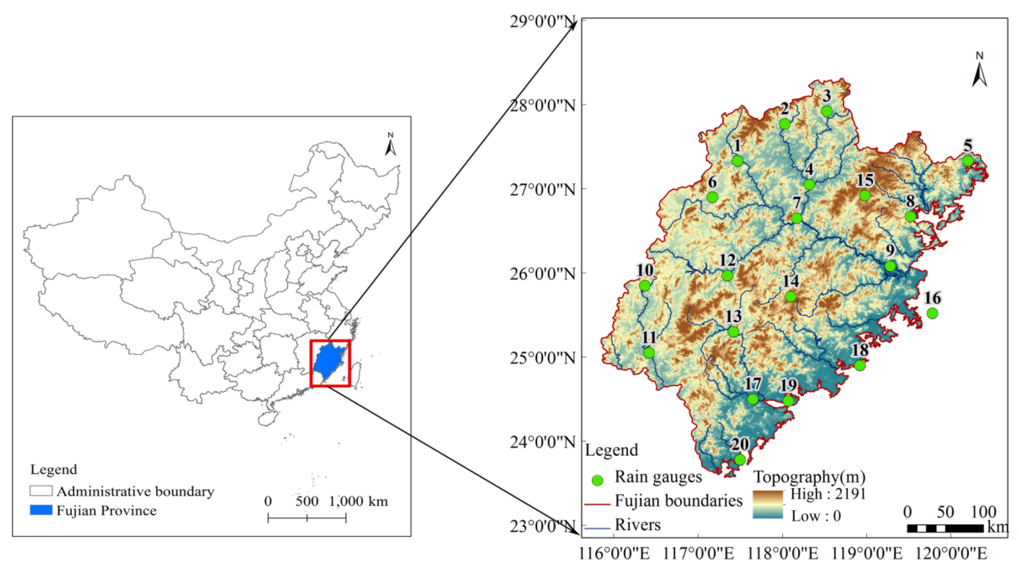
2.1. Study Area

The present study focused on Fujian province, which lies along the southeastern coast of China, covering an area of approximately 120,000 km², with relevant coordinates ranging from 115°50′E to 120°47′E and from 23°30′N to 28°19′N (Figure 1). The maximum dimensions of the area are approximately 480 km (east to west) and 530 km (north to south). The area’s climate is representative of a typical subtropical monsoon climate with abundant rainfall. The average annual rainfall is between 1400 and 2000 mm, with an overall trend of decreasing rainfall from the northwest to the southeast part of the area. The temporal distribution of rainfall over Fujian province exhibits apparent seasonal differences, including characteristically wet (March through September) and dry (October through February) seasons. Most rainfall occurs during the rainy season, which accounts for about 80% to 90% of the annual rainfall.

Figure 1. Location map of Fujian province showing the distribution and locations of the 20 rain gauge stations within the area.

Figure 1. Location map of Fujian province showing the distribution and locations of the 20 rain gauge stations within the area.

2.2. Rain Gauge Data

The ground-based observations used in the present study were collected by the China Meteorological Data Sharing Service System [43]. Specifically, the available dataset consisted of daily rainfall records obtained during the time period 2000 to 2012 at the 20 rain gauges scattered across Fujian province (Figure 1). The statistical information about the annual and monthly rainfalls obtained from the daily rainfall records is displayed in Table 1 and Table 2. For comparative analysis purposes, the data used to perform the monthly interpolation of the rain gauge data were the average monthly rainfall observations at the 20 stations during the 13-year period. These rain gauge data were used for ground truthing, and they were defined as the primary variable X suitable for spatiotemporal interpolation purposes.

Table 1. Statistics for the dataset of the annual rainfall from 20 rain gauge stations.

Statistical Magnitude	Values	Statistical Magnitude	Values
Count a	260	Standard deviation	419.03 (mm)
Minimum	689.5 (mm)	Median	1585.38 (mm)
Maximum	2849.35 (mm)	Skewness	0.26
Mean	1602.99 (mm)	Kurtosis	2.56

^a Count: number of annual/monthly rain gauge data (20 stations × 13 years = 260 samples or 20 stations × 13 years × 12 months = 3120 samples).

Table 1. Statistics for the dataset of the annual rainfall from 20 rain gauge stations.

Statistical Magnitude	Values	Statistical Magnitude	Values
Count a	260	Standard deviation	419.03 (mm)
Minimum	689.5 (mm)	Median	1585.38 (mm)
Maximum	2849.35 (mm)	Skewness	0.26
Mean	1602.99 (mm)	Kurtosis	2.56

^a Count: number of annual/monthly rain gauge data (20 stations × 13 years = 260 samples or 20 stations × 13 years × 12 months = 3120 samples).

Table 2. Statistics for the dataset of monthly rainfall from 20 rain gauge stations.

Statistical Magnitude	Values	Statistical Magnitude	Values
Count	3120	Standard deviation	117.81 (mm)
Minimum	0 (mm)	Median	124.55 (mm)
Maximum	886.75 (mm)	Skewness	1.6239
Mean	134.23 (mm)	Kurtosis	6.4883

Table 2. Statistics for the dataset of monthly rainfall from 20 rain gauge stations.

Statistical Magnitude	Values	Statistical Magnitude	Values
Count	3120	Standard deviation	117.81 (mm)
Minimum	0 (mm)	Median	124.55 (mm)
Maximum	886.75 (mm)	Skewness	1.6239
Mean	134.23 (mm)	Kurtosis	6.4883

2.3. Satellite Rainfall Data (TRMM 3B42)

TRMM estimates tropical precipitation from space sensors using a suite of rain retrieval algorithms. The TRMM 3B42 estimates that were employed in this study are produced at a temporal resolution of 3 h and a spatial resolution of 0.25°. The major inputs to the TRMM 3B42 algorithm are infrared estimates from geostationary satellites and microwave estimates from the TRMM microwave imager (TMI), special sensor microwave imager (SSM/I), Advanced Microwave Sounding Unit (AMSU) and Advanced Microwave Sounding Radiometer-Earth Observing System (AMSR-E) [44].

The TRMM 3B42 estimates were produced in four phases [44]: (1) the microwave estimates are calibrated and combined; (2) infrared estimates are created using the calibrated microwave rainfall data; (3) both estimates are combined; and (4) an indirect rescaling to monthly ground data is applied. In this study, the TRMM 3B42 dataset covering the study area was downloaded from Goddard Earth Sciences Data and Information Services Center. The daily aggregated rainfall was obtained by summing all eight sets of 3-h rainfall totals for a given day, as were the monthly and annual aggregated rainfall. These preprocessed TRMM 3B42 estimates were subsequently defined as the secondary variable Y in the relevant interpolation methods.

3. Methods

In this study, data verification was carried out on the rain gauge data for consistency analysis, and the validation of TRMM 3B42 estimates was implemented for quality assessment in Fujian province before space-time interpolation and comparative analysis.

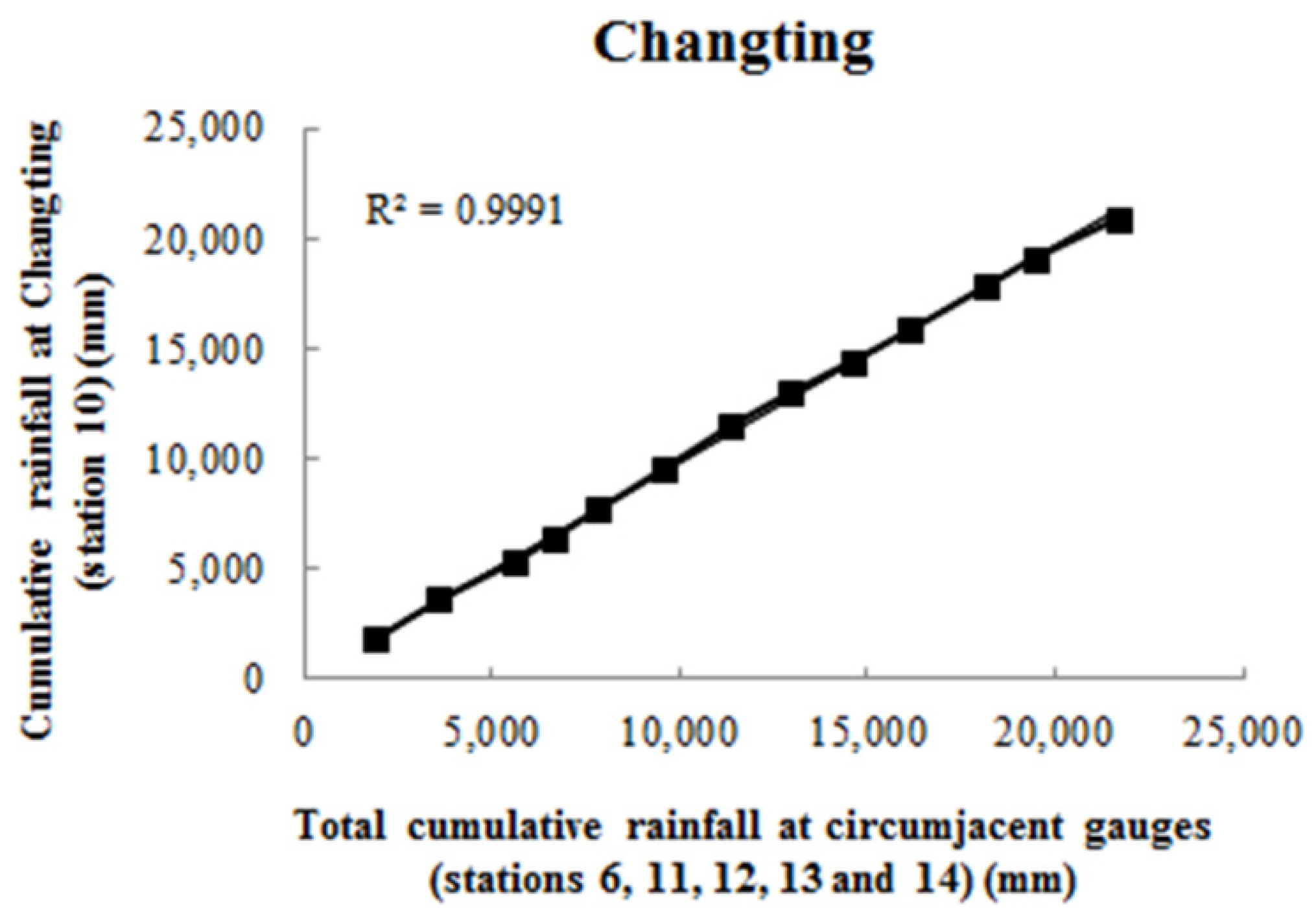
3.1. Consistency Analysis of Rain Gauge Data

In order to ensure that the trends in the observations are due to meteorological causes rather than to changes in gauge location, equipment location or observational method, it was necessary to perform rain gauge data consistency checks. DMC (double-mass curve) analysis [45] was employed to check and adjust inconsistency in the rain gauge record. DMC theory is based on the fact that a plot of the two cumulative quantities (i.e., rainfall accumulation at a given station and average accumulation for a group of surrounded stations) during the same period follows a straight line so long as the proportionality between the two remains unchanged, in which case the slope of the line represents this proportionality [46]. A break in the DMC slope means that a change in the constant of proportionality between the two variables has occurred or, perhaps, that the proportionality is not a constant at all rates of accumulation. In hydrologic studies, DMC is often represented by a plot of two variables: the rainfall accumulation at a given station and the average accumulation at a group of surrounded stations. The consistency of rain gauge records was checked by examining the tendency of the DMC slope, and adjustments for inconsistencies were carried out according to the equation:

$$P^{\prime }=\frac{\text{tan}{\text{α}}^{\prime }}{\text{tan}\mathrm{\alpha }}P$$

(1)

where P is the rainfall observation, P^' is the adjusted rainfall, tan ɑ is the slope of the original DMC and tan ɑ^' is the slope of the inconsistent section of the DMC [45].

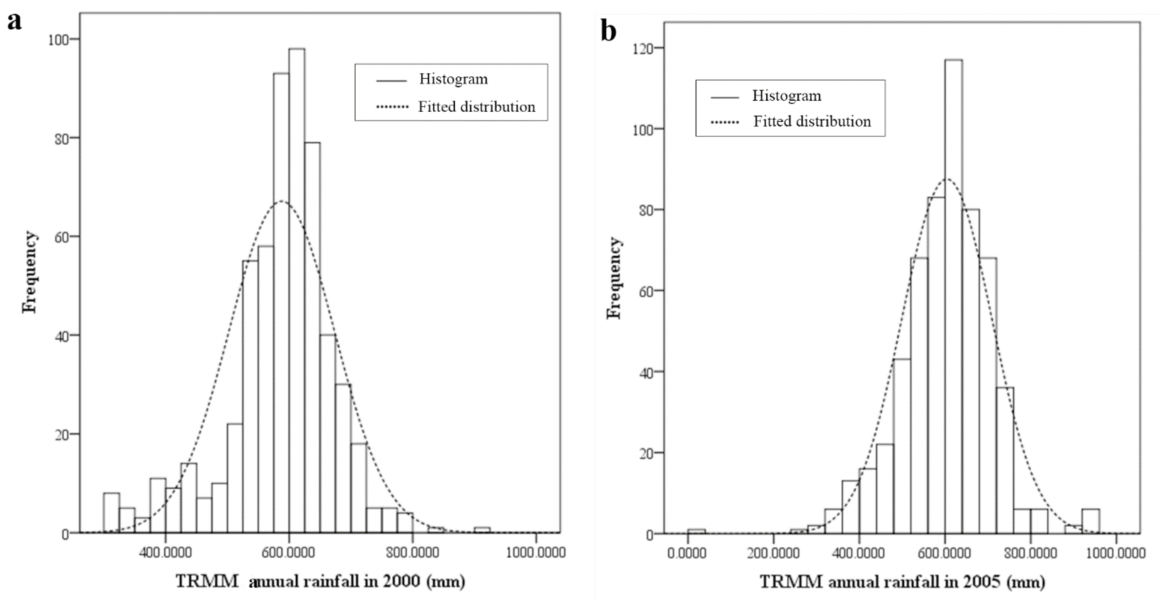
3.2. Validation of TRMM 3B42 Estimates and Soft Data Modeling

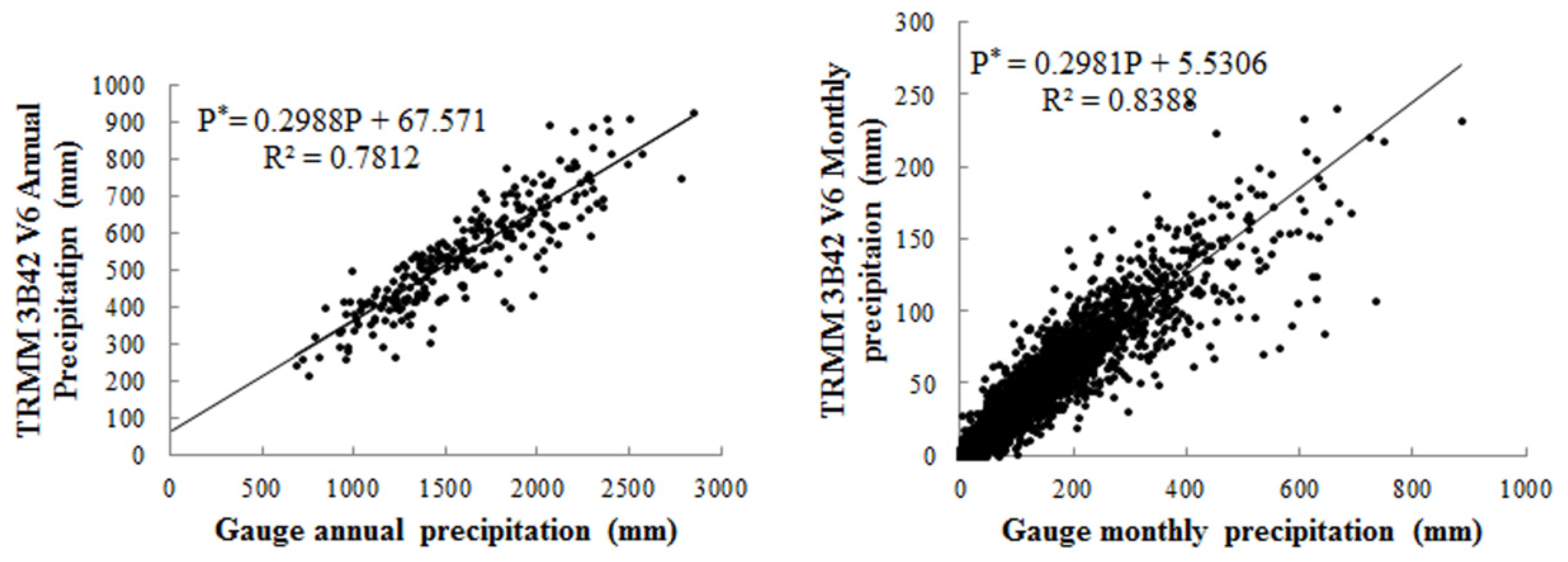
3.2.1 Validation of TRMM 3B42 Estimates

The accuracy and reliability of TRMM rainfall estimates have been assessed in recent studies [47,48,49]. However, the performance of the TRMM estimates varies from place to place. Hence, it is always necessary to evaluate the performance and accuracy of TRMM estimates with rain gauge data, before using them for localized applications.

Generally, for localized accuracy and reliability assessments, TRMM rainfall estimates should be calibrated and validated using rain gauge networks that are considered to be accurate. In this study, a validation approach was proposed for the TRMM 3B42 estimates against the ground-based rain gauge measurements within Fujian province at the monthly and annual temporal scales, for 13 concurrent years (2000 to 2012). The coefficient of determination, which is the square of the correlation coefficient (R) of the best fit linear regression line, was used to compare the statistical fit of the TRMM 3B42 estimates to the ground-based rain gauge data.

3.2.2 Soft Data Modeling

Some disagreement between satellite data and rain-gauge data is, however, expected because of the very different sampling patterns of the two systems: the satellite provides only occasional snapshots of large areas, whereas rain gauges provide continuous measurements over very small areas. Thus, two steps were performed in order to improve interpolation accuracy. Firstly, based on the existing correlation between TRMM 3B42 estimates and rain gauge data, a linear regression line was fitted between the two during the period 2000 to 2012, at the annual and the monthly scales. This resulted in an empirical model of the form:

$$P^{*}=aP+b$$

(2)

where P^* is the fitted annual or monthly TRMM rainfall estimate, P is the rain gauge annual or monthly rainfall measurement and a, b are regression coefficients.

Secondly, the fitted TRMM data P* were used to generate the probabilistic soft data. The soft data were expressed in terms of Gaussian distributions, because of the good fit of these distributions to the P^* values. For illustration, the fitted distribution and the histogram plots for two years are displayed in Figure 2. Then, soft datasets of annual and monthly TRMM rainfall were calculated in the study area between 2000 and 2012. The mean and variance were given by, respectively,

$$\mu =\frac{1}{n}{\displaystyle {\sum }_{i=1}^n{P}_i^{*}}$$

(3)

$${\sigma }^2=\frac{1}{n}{\displaystyle {\sum }_{i=1}^n{(P_i^{*}-\mu )}^2}$$

(4)

where i is the number of the year or month and n is the total number of years or months considered.

Figure 2. Histogram of TRMM annual estimates and fitted Gaussian distribution in 2000 (a) and 2005 (b).

Figure 2. Histogram of TRMM annual estimates and fitted Gaussian distribution in 2000 (a) and 2005 (b).

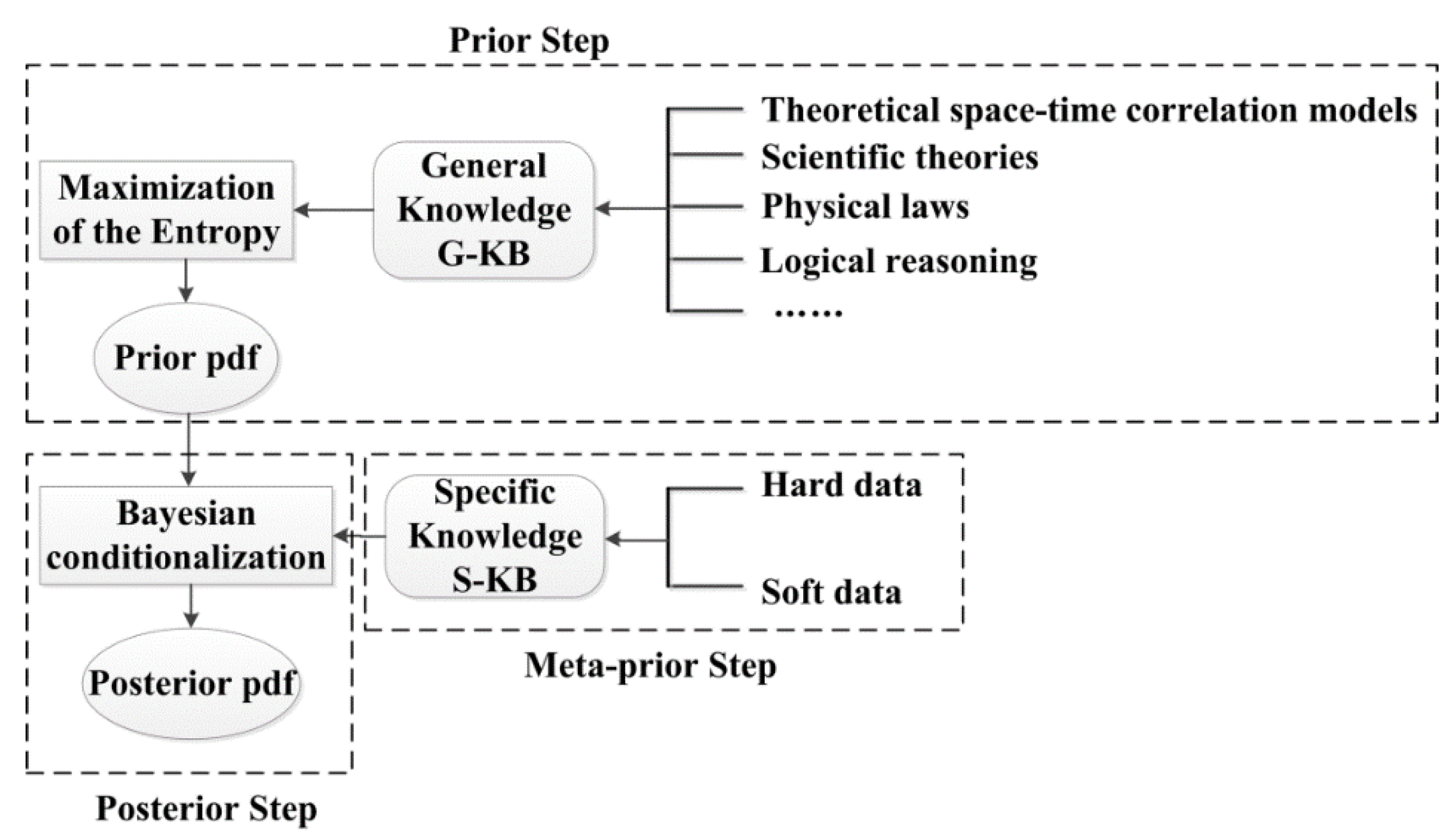
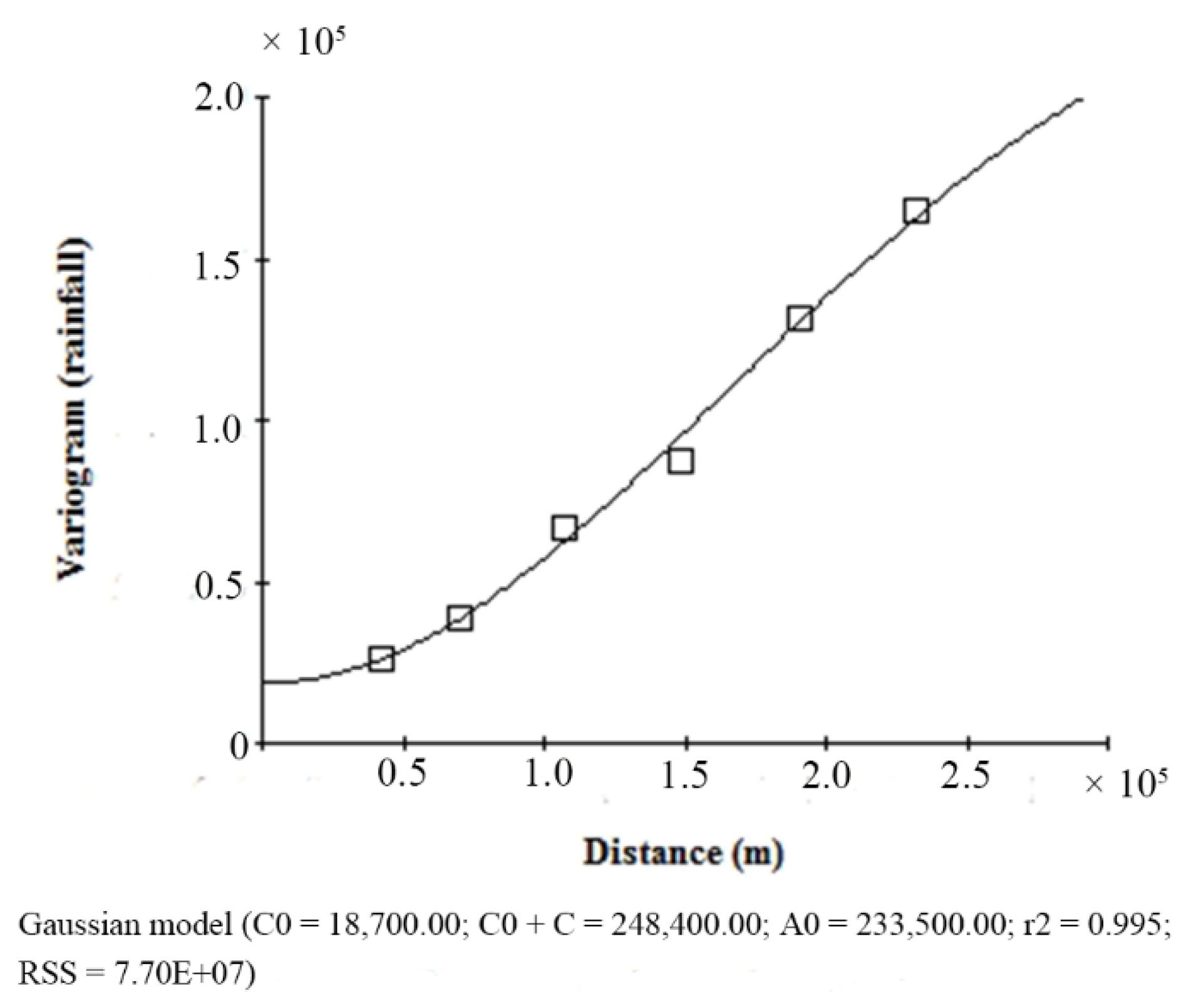
3.3. Spatiotemporal BME Analysis

Many space-time interpolation techniques, such as cokriging (CK), account for secondary hard data using the statistical cross-correlation between the primary and the secondary variables. However, they do not account for secondary variables linked to the primary variable by means of an empirical law in uncertain in situ conditions, which can be used to generate useful soft data. On the other hand, the BME spatiotemporal mapping method can account for empirical laws and soft data, such as above, in a mathematically-rigorous and physically-meaningful manner. The soft data, in particular, may take the form of interval values, fuzzy sets and probability functions and subsequently used by BME to improve space-time modeling and estimation.

Figure 3. Flow chart of the Bayesian maximum entropy (BME) method. G-KB, general knowledge base; S-KB, site-specific KB.

Figure 3. Flow chart of the Bayesian maximum entropy (BME) method. G-KB, general knowledge base; S-KB, site-specific KB.

The main methodological steps of BME are shown in Figure 3: The first step derives the prior probability density function (pdf), f_G(P), of rainfall P that is maximally informative, given the available G-KB that is mathematically expressed by the vector function g. In this paper, mean and covariance functions are used as general knowledge (known as G-KB). In fact, mean and covariance functions represent trends and spatial/spatiotemporal interactions (dependencies) of data, respectively. G-KB is described by spatial/spatiotemporal covariance, which is fully based on observed rainfall values. In the second step, the S-KB concerning the phenomenon of interest (including hard data and soft data) is collected and translated into the mathematical functions ξ_S. In this study, soft data of rainfall are assumed to be in the shape of probability functions. In the final step, the posterior (conditional) pdf, f_K(P), is obtained based on the integration of the prior pdf f_G(P) derived in the first step and the site-specific function ξ_S developed in the second step. The posterior rainfall pdf f_K(P) is then calculated in terms of the solution of the set of equations [10]:

$$\int dP(\mathit{g}-\overline{g})f_G\left(P\right)=0$$

(5)

$$\int dP{\xi }_S{f}_G\left(P\right)-A\left[f_K\right(P\left)\right]=0$$

(6)

where $\overline{g}$ denotes the mean value of the vector function g; and A is a normalization parameter. The spatiotemporal BME method has a number of attractive features compared to mainstream interpolation techniques, like geostatistical kriging:

-

It makes no restrictive assumptions concerning the linearity and normality of the interpolator (nonlinear interpolators and non-Gaussian laws are automatically incorporated).

-

It can synthesize various kinds of KBs (core and site-specific) in a general and unified manner, and it can readily consider uncertain yet valuable information at the interpolation points themselves, when available.

-

It offers a more sound characterization in terms of the complete estimation pdf at every space-time point. These pdf may have different shapes (non-Gaussian, in general). Based on the pdf one, can calculate a number of possible rainfall estimates (mean, mode, median, etc.) with their associated probabilities, accuracies and confidence intervals.

-

It derives certain mainstream geostatistics and space-time statistics techniques (e.g., statistical regression and kriging) as its special cases, thus demonstrating BME’s generalization power (e.g., when the G- and the S-KB are restricted to a two-point variogram and hard data, respectively, the BME obtains OK as its special case).

3.4. Model Evaluation

The cross-validation method is used to select the best variogram model among several candidates (the variogram models chosen for this study are discussed in Section 4.3.1 below). Accordingly, the accuracy of the candidate models was measured by the mean absolute error (MAE), which is a measure of the sum of the absolute residuals (estimated-actual values), and the root mean square error (RMSE), which is the square root of the sum of the squared residuals. Small MAE values indicate a model with few errors, whereas small RMSE values indicate more accurate estimates on a point-by-point basis.

Numerically, the MAE and RMSE values are calculated, respectively, by:

$$MAE=\frac{{\displaystyle {\sum }_{i=1}^n|{\widehat{P}}_i-P_i|}}{n}$$

(7)

and:

$$RMSE=\sqrt{\frac{{\displaystyle {\sum }_{i=1}^n{({\widehat{P}}_i-P_i)}^2}}{n}}$$

(8)

where n is the number of sample stations used in the validation sets, P_i are the observed values and ${\widehat{P}}_i$ are the estimated values.

4. Results and Discussion

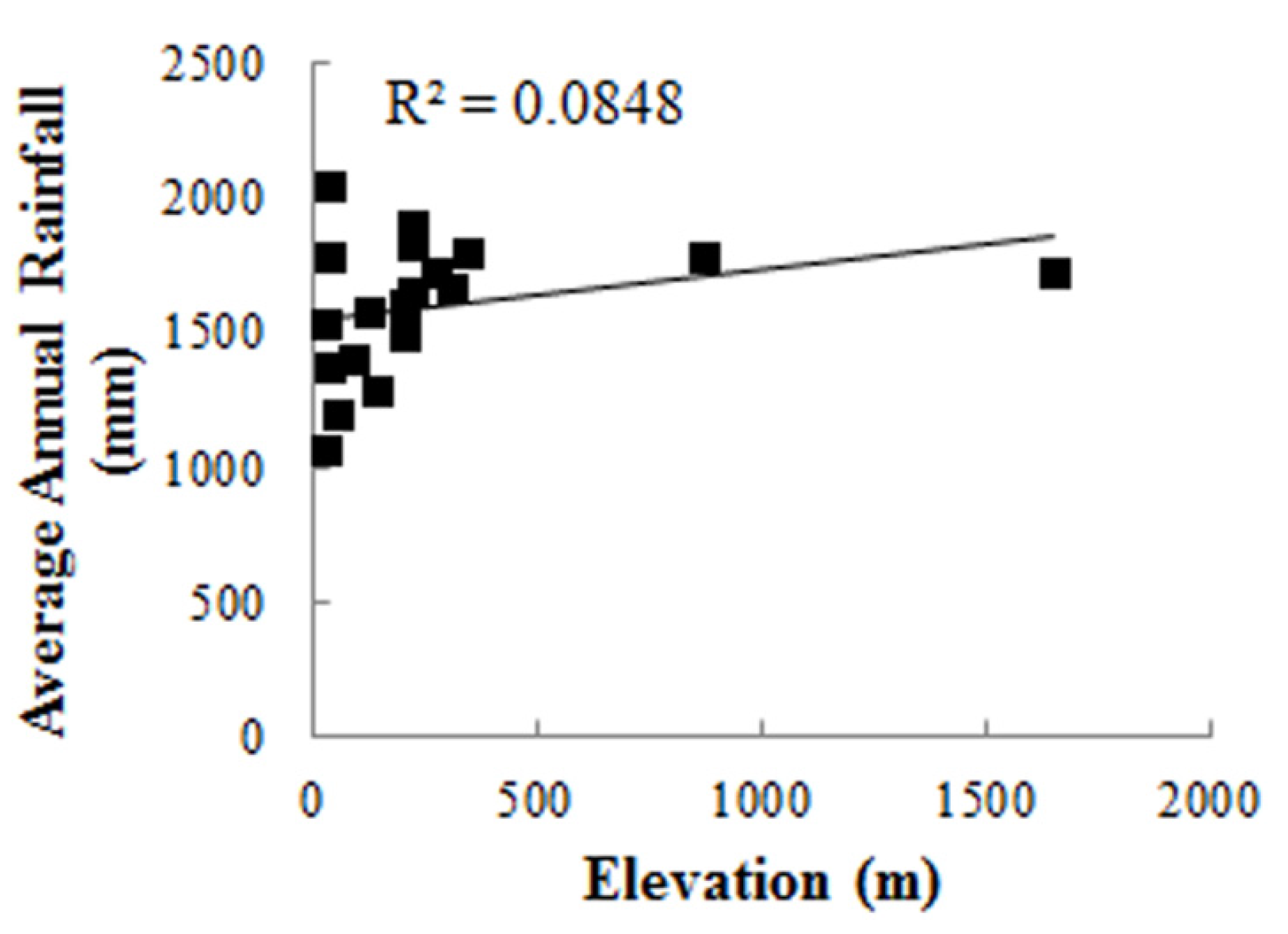
4.1. Rain Gauge Data Consistency Results and Analysis

For illustration purposes, Figure 4 shows the results of the DMC analysis at the Changting rain gauge station, in which the horizontal axis denotes the cumulative average annual rainfall of five rain gauge stations around Changting and the vertical axis denotes the cumulative rainfall at the Changting station during 13 years. These results demonstrated the very high consistency of the Changting rain gauge station. Results for other gauge-measured rainfall generally showed similarly high consistencies with minimum and maximum R² values of 99.6% and 99.9%.

Specifically, the DMC results for all stations show that the records are consistent at all 20 stations identified in Figure 1, although the points scatter slightly on both sides of the line. This implies that the observed marginal differences in gauge-based data were not the result of meteorological influences. Therefore, there are no inconsistencies to be adjusted for the candidate 20 gauge stations during the 13 years considered in the present study.

Figure 4. Double-mass curve for Changting rain gauge station (the locations of the station numbers can be seen in Figure 1).

Figure 4. Double-mass curve for Changting rain gauge station (the locations of the station numbers can be seen in Figure 1).

4.2. Evaluation of TRMM 3B42 Estimates

Figure 5 shows scatter plots and linear regression equations (with 99% significance) of data from rain gauge stations vs. TRMM 3B42 estimates at two temporal scales, annual and monthly. Excellent agreement with the rain gauge data was observed for the TRMM 3B42 estimates at both annual and monthly scales with R² values equal to 0.78 and 0.84, respectively. However, the TRMM 3B42 estimates were overall slightly smaller than the rain gauge observed values. This result is probably related to spatiotemporal inconsistencies between TRMM 3B42 estimates and ground-based rain gauge data. TRMM/TMI data products are the retrieval results of observed microwave brightness temperature, combined with a cloud numerical model and a radiative transfer model. The underlying surface background radiation has an impact on the TMI retrievals. For example, the TMI overestimates deep convective rain and stratiform rain, whereas it underestimates shallow convective rain [50]. Accordingly, the underestimation of TRMM 3B42 in the Fujian area is likely caused by its shallow convective rain [51]. However, the high consistency of rain gauge data and TRMM 3B42 estimates indicates that the rainfall of the TRMM 3B42 estimates is reliable at both the annual and the monthly scales.

Figure 5. Scatter plots of annual (left) and monthly (right) rainfall at 20 rain gauge stations vs. TRMM 3B42 estimates (2000 to 2012).

Figure 5. Scatter plots of annual (left) and monthly (right) rainfall at 20 rain gauge stations vs. TRMM 3B42 estimates (2000 to 2012).

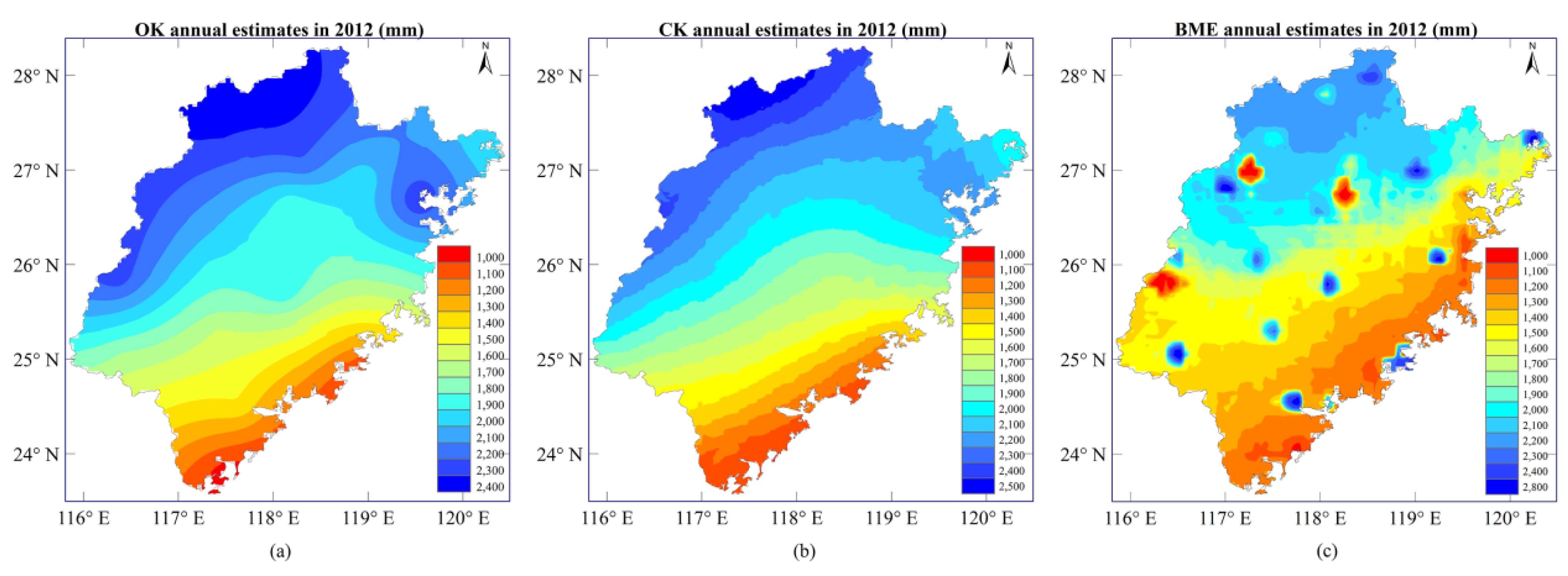
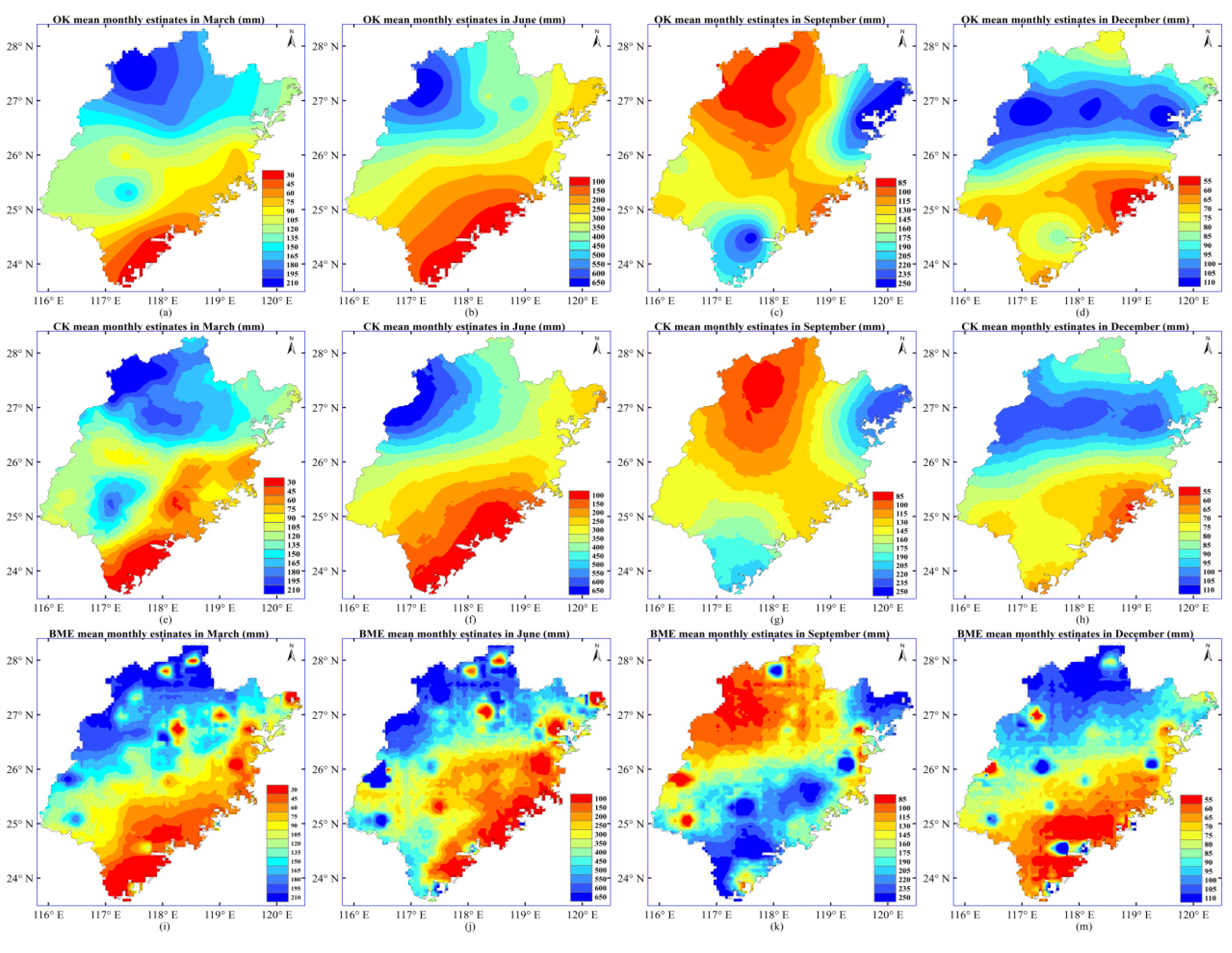
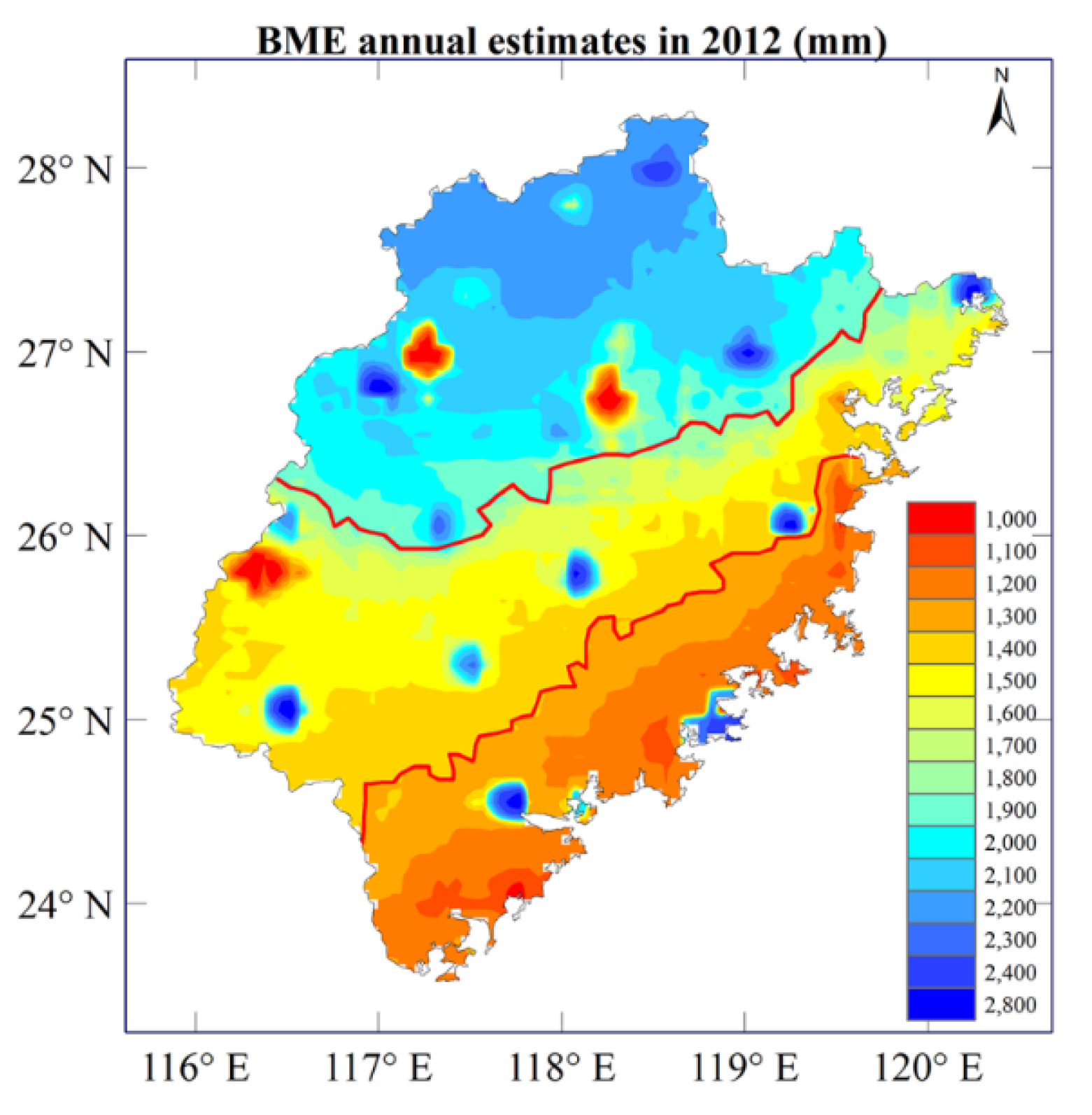
4.3. Comparative Spatiotemporal Rainfall Mapping

Figure 6 shows the correlation between average annual rainfall from 2000 to 2012 and the elevation of the 20 stations. The correlation coefficient (R) between the graphs of two datasets is only about 0.29.

Figure 6. The relationship between average annual rainfall (y) and elevation (x) before estimation.

Figure 6. The relationship between average annual rainfall (y) and elevation (x) before estimation.

Due to the low-level spatiotemporal correlation between elevation and the average annual rainfall calculated in the study area, the effect of altitude on rainfall was not considered in this work. This means that spatiotemporal mapping can focus on annual and monthly rainfalls over the entire study area according to the aforementioned data analysis by means of the BME-TRMM method. Then, the results can be compared to those of the OK and CK techniques. In order to facilitate the discussion, below, we present and discuss the comparisons separately (OK vs. CK vs. BME, monthly vs. annual rainfall, etc.).

4.3.1. Spatiotemporal Distribution of Annual Rainfall

Since one of the goals of the present study is to compare the performance of different space-time modeling and mapping techniques, the annual rainfall dataset for the entire period of study consisted of two parts:

(1) Primary hard data (observations at 20 stations during 13 years), X_a-hard, and the secondary hard data, Y_a-hard (fitted annual TRMM data obtained by the empirical model of Equation (2)).

(2) Soft data of the Gaussian probabilistic form, Y_a-soft, computed by Equations (3) to (4) with input parameters the TRMM data obtained from Equation (2).

Experimental variograms were calculated based on the hard data above, using standard geostatistics [52]. Then, primary fitting of experimental variograms (primary theoretical variogram) was carried out using the GS + software. The resulting experimental variogram together with the fitted theoretical variogram (Gaussian model) are plotted in Figure 7. The parameters of the Gaussian model were calculated based on the goodness of fit (maximum correlation coefficient) criterion, as follows: nugget = 18,700, sill = 248,400 and range = 404,433. The parabolic shape of the variogram at the lag origin indicates a rather smooth variation of the rainfall values across space.

Figure 7. Experimental variogram (squares) and theoretical (Gaussian) variogram (continuous line) for annual rainfall.

Figure 7. Experimental variogram (squares) and theoretical (Gaussian) variogram (continuous line) for annual rainfall.

In the OK method, only X_a-hard were directly used to interpolate and generate rainfall prediction maps. In the CK method, a linear combination of data including X_a-hard and Y_a-hard was used in rainfall interpolation. Finally, the BME mapping method incorporated X_a-hard and a set of probabilistic soft data Y_a-soft to account for the empirical relationship of Equation (2). For illustration purposes, Figure 8 shows the annual rainfall maps during 2012 generated by the three methods.

Figure 8. A subset of ordinary kriging (OK) (left), cokriging (CK) (middle) and BME (right) annual rainfall maps (year 2012).

Figure 8. A subset of ordinary kriging (OK) (left), cokriging (CK) (middle) and BME (right) annual rainfall maps (year 2012).

Comparing the rainfall maps (OK, CK, BME) in Figure 8, it is clear that all three maps display a definite rainfall pattern over the region: rainfall decreases progressively from the northwestern mountains to the southeastern coast. One can observe a rather uneven spatial distribution of rainfall values with significant differences in magnitude. High rainfall occurs in the regions between 117° and 119° longitude and 27° and 28° latitude with average annual rainfall exceeding 2000 mm, whereas low values occur between 117° and 119° longitude and 23° and 25° latitude with average annual rainfall below 1500 mm. Intermediate values occur in the middle region with average annual rainfall between 1500 and 1700 mm.

The spatial distribution of the OK rainfall estimates is represented by a continuous and smooth surface, which, though, does not accurately represent the thermal and dynamic forcing mechanisms of the local topography. In contrast, the map produced by the BME method is more informative, represented by a surface with reduced smoothness (compared to the maps produced by OK and CK) and reflecting accurately the local variations of rainfall throughout the region.

4.3.2. Spatiotemporal Distribution of Monthly Rainfall

Similar to the annual rainfall dataset, the monthly rainfall datasets were grouped into hard and soft data. The monthly hard data, X_m-hard, consisted of average monthly rainfall values at 20 stations during a 13-year period, and the average fitted monthly TRMM data, Y_m-hard. The monthly rainfall soft data, Y_m-soft, were calculated from Equations (3) and (4) based on TRMM average monthly rainfall estimates.

Figure 9 shows the results obtained by the three methods of rainfall mapping considered in this work (OK, CK and BME). What the three methods share is that they all provide valuable space-time visualizations of the considerable geographical variation and temporal seasonality of rainfall throughout the study region. The change in the spatial rainfall pattern from month to month is clearly depicted in all maps. The spatial trend in the rainfall distribution decreases from the northwest to the southeast, with the maximum exceeding 200 mm during spring (March to May), whereas an inverse trend is evident during autumn (September to November). Abundant rainfall was observed throughout the region with the maximum value (>600 mm) occurring during the summer months (July to August), whereas the opposite is true during the winter months (December to January). Variation in the temporal rainfall pattern is also clearly visible, with much higher rainfall levels during spring and summer and much lower rainfall levels during autumn and winter. Important differences between the three methods of space-time modeling and interpolation are also evident in the maps.

Figure 8 and Figure 9 also show that the BME-TRMM model predicts noticeable spikes (high levels) of rainfall at individual stations surrounded by much lower rainfall estimates. These spikes appear because of the dense gradient between them and the values at the surrounding grid nodes. We consider these isolated high levels as a natural consequence of the significant spatial heterogeneity of the observations (at the specified stations and at neighboring points). To test the spatial rainfall heterogeneity, the q-statistic [53] approach was applied to the BME results with three strata partitioned by rainfall. The results are presented in Figure 10. The q-statistic approach is used to measure the degree of spatially-stratified heterogeneity and to test its significance. There are many spatially-stratified heterogeneous phenomena, such as administrative units, differences in the population densities in different areas, climates or ecological zones or the distribution of soil types, land use and land cover.

Unlike OK, the BME successfully identifies important local variations in the rainfall distribution. Furthermore, the theoretical differences between the three space-time methods lead to quantitative differences between the OK, CK and BME maps of rainfall distribution, which are assessed numerically in the following section.

Figure 9. A subset of OK (top), CK (middle) and BME (bottom) mean monthly rainfall maps (month of March, June, September and December, from left to right).

Figure 9. A subset of OK (top), CK (middle) and BME (bottom) mean monthly rainfall maps (month of March, June, September and December, from left to right).

Figure 10. Spatial heterogeneity of BME rainfall estimates in the Fujian area in 2012. Red lines divide the data into three strata, q = 0.67*** (p = 2.13 × 10⁻⁵). p is the probability of q-statistic; the value of the statistic must be within [0, 1], where zero denotes zero spatial heterogeneity and one denotes complete heterogeneity; *** denotes statistical significant at level smaller than 10⁻³.

Figure 10. Spatial heterogeneity of BME rainfall estimates in the Fujian area in 2012. Red lines divide the data into three strata, q = 0.67*** (p = 2.13 × 10⁻⁵). p is the probability of q-statistic; the value of the statistic must be within [0, 1], where zero denotes zero spatial heterogeneity and one denotes complete heterogeneity; *** denotes statistical significant at level smaller than 10⁻³.

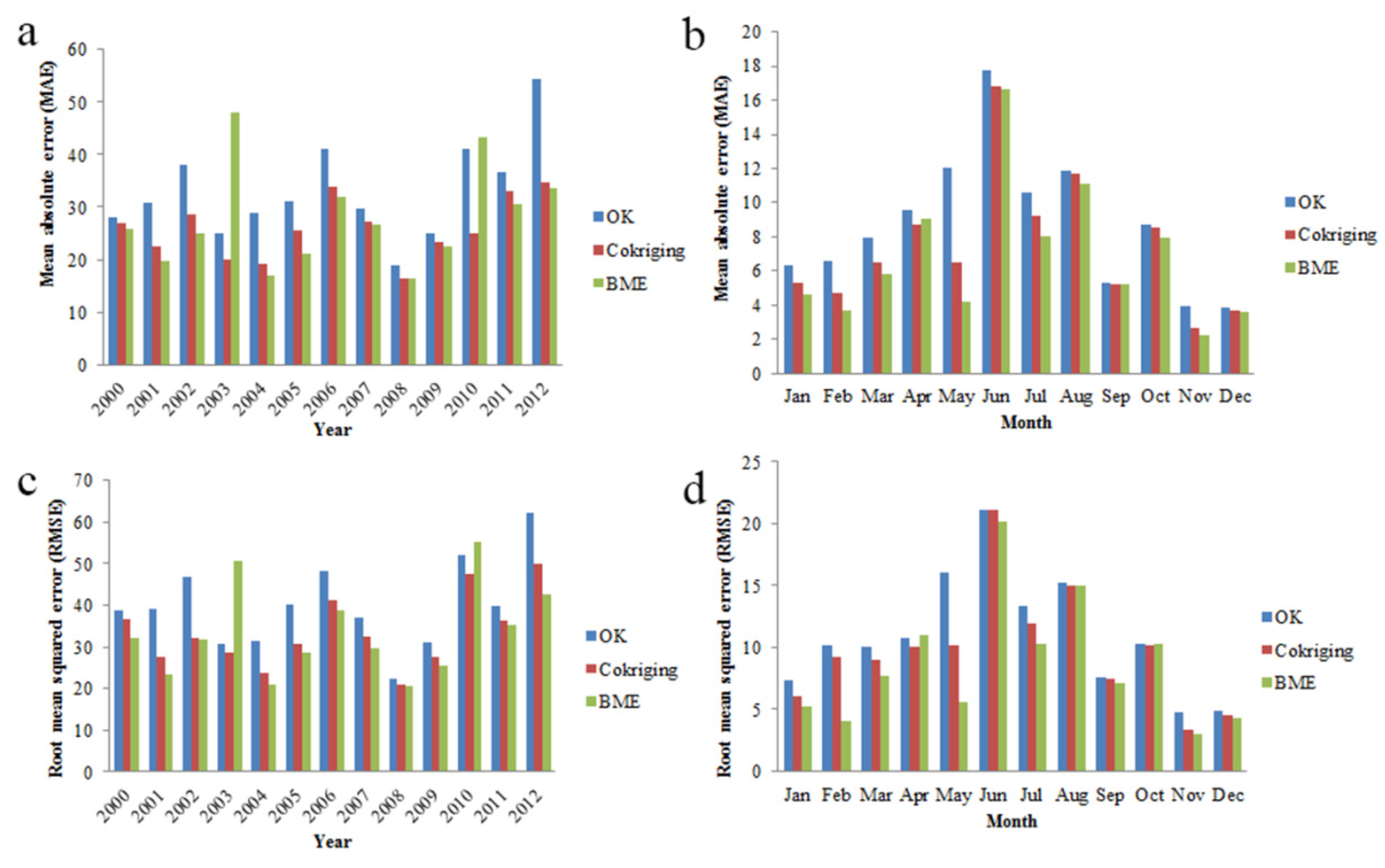
4.4. Cross-Validation Assessment Results

In this section, the observations obtained by rain gauges are used to validate the results obtained by the three methods. BME’s performance is further assessed by comparing it to the commonly-used OK and CK interpolation methods.

The results of the cross-validation approach are shown in Figure 11. In this figure, the left and right columns display annual and monthly rainfall estimates, respectively. Overall, there are no considerable differences between the results of the three methods. As is seen in Figure 11a and c, compared to OK, the CK with TRMM as a covariant leads to lower MAE and RMSE values during all years considered, which indicates that the CK-TRMM performs better than OK in estimating annual rainfall in Fujian province. This happens because the TRMM estimates effectively complement the rainfall observations. On the other hand, the BME with TRMM as soft data performs better than CK during most years, except for the years 2003 and 2010, when BME-TRMM gives higher (2003) or similar (2010) MAE and RMSE values compared to those of given by CK-TRMM. To gain some computational insight, the absolute error of the BME estimates was compared to that of the CK estimates at each station during the years 2003 and 2010. It was found that the absolute BME interpolation error was rather high at some stations. As it turned out, this was due to the inadequate fit between the TRMM estimates and the gauge data for the specific two years that were subsequently used as an input to BME. Indeed, following a careful analysis of the results of the linear regression model fitted to the auxiliary variable TRMM estimates vs. the host variables rain gauge data, it was found that the relative error was high in the years 2003 and 2010 compared to the errors during the other years (although the coefficient of determination, R2, of the model was very high). In addition, the stations used for modeling purposes were too few to provide accurate fit results; therefore, when these results were converted into the soft format used in BME mapping, the absolute error of the estimated values was particularly high at some stations.

Figure 11. Results of the cross-validation approach for annual/monthly rainfall for (a) MAE-annual, (b) MAE-monthly, (c) RMSE-annual and (d) RMSE-monthly.

Figure 11. Results of the cross-validation approach for annual/monthly rainfall for (a) MAE-annual, (b) MAE-monthly, (c) RMSE-annual and (d) RMSE-monthly.

Similar conclusions were drawn regarding the MAE and RMSE values of the monthly rainfall estimated by OK, CK and BME between January and December of 2002 (see Figure 11b,d). Moreover, the same trend in the MAE and RMSE values was observed in the annual rainfall results. All of the comparisons above show that, in general, BME-TRMM produces more accurate rainfall estimates than CK-TRMM and OK over the region of interest.

In summary, based on the numerical comparisons above, the two evaluation criteria demonstrated the considerable advantage of using TRMM estimates to complement rain gauge data deficiencies. It was also shown that the BME-TRMM technique produces results that are clear improvements in rainfall estimation in Fujian province compared to the OK and CK techniques (e.g., BME-TRMM generated realistic and more accurate spatiotemporal rainfall maps in most years and months, with the exception of two years in which estimation suffered from soft data inadequacy).

5. Conclusions

TRMM 3B42 rainfall estimates were validated in terms of ground observations at 20 independent rain gauges, and soft data derived from TRMM 3B42 rainfall estimates were generated by regression modeling. The spatiotemporal patterns of annual and monthly rainfall between the years 2000 and 2012 were analyzed by BME, which adequately integrates hard data from the 20 rain gauge data with the soft TRMM 3B42 estimates mentioned above. The study of the BME-TRMM maps revealed the existence of spatiotemporal rainfall trends in Fujian region. Firstly, there is a distinct spatial variation in the rainfall levels throughout the region of interest. The different interpolation techniques considered in the present work revealed strong regional trends, with a rainfall decrease from the northwest to the southeast parts of the region. Secondly, annual rainfall fluctuations were clearly observed (in the Fujian region, the rainfall amount varied between 690 and 2800 mm/year.). Secondly, seasonal patterns were very strong, with rainfall differences between the dry and wet seasons exceeding 500 mm. An increasing trend is observed from March to August, with most rainfall occurring during May and June. Lastly, a decreasing rainfall trend occurs between September and December.

The performance of the combined BME-TRMM method was further assessed by comparing it to the commonly-used OK and CK techniques. It was demonstrated that TRMM rainfall estimates (covering most parts of the Earth) can improve spatiotemporal interpolation accuracy by effectively complementing the low density of rain gauge networks. BME with TRMM as soft data offered a more realistic picture of the phenomenon by accounting for more local variations than did OK and CK, at both the annual and monthly scales. The MAE and RMSE results showed that the rainfall maps generated by the BME-TRMM method are more accurate and informative than those generated by the OK method and also superior to those produced by the CK method with TRMM as a covariant, during most years and months.

In sum, the comparative analysis of the three methods considered in this work demonstrates that rainfall interpolation reliability can be improved by accounting for satellite-derived estimates (e.g., TRMM estimates). Furthermore, the analysis shows that the BME method with TRMM as soft data has certain advantages in the modeling and mapping of spatiotemporal rainfall patterns.

References

1. Beven, K.J. Rainfall-Runoff Modelling: The Primer, 2nd ed.; John Wiley & Sons: Chichester, UK, 2011. [Google Scholar]
2. Thiessen, A.H. Precipitation averages for large areas. Mon. Weather Rev. 1911, 39, 1082. [Google Scholar] [CrossRef]
3. Dingman, S.L. Physical Hydrology, 2nd ed.; Prentice Hall: Upper Saddle River, NJ, USA, 2002. [Google Scholar]
4. Tabios, G.Q.; Salas, J.D. A comparative analysis of techniques for spatial interpolation of precipitation1. J. Am. Water Resour. Assoc. 1985, 21, 365–380. [Google Scholar] [CrossRef]
5. Parajka, J. Mapping long-term mean annual precipitation in slovakia using geostatistical procedures. In Proceedings of the International Conference on Problems in Fluid Mechanics and Hydrology, Prague, Czech Republic, 23–26 June 1999; pp. 424–430.
6. Basistha, A.; Arya, D.; Goel, N. Spatial distribution of rainfall in indian himalayas—A case study of uttarakhand region. Water Resour. Manag. 2008, 22, 1325–1346. [Google Scholar] [CrossRef]
7. Wang, J.-F.; Stein, A.; Gao, B.-B.; Ge, Y. A review of spatial sampling. Spat. Stat. 2012, 2, 1–14. [Google Scholar] [CrossRef]
8. Christakos, G. A bayesian/maximum-entropy view to the spatial estimation problem. Math. Geol. 1990, 22, 763–777. [Google Scholar] [CrossRef]
9. Christakos, G. Random Field Models in Earth Sciences; Academic Press: New York, NY, USA, 1992. [Google Scholar]
10. Christakos, G. Modern Spatiotemporal Geostatistics; Oxford University Press: Oxford, UK, 2000. [Google Scholar]
11. Christakos, G.; Bogaert, P.; Serre, M.L. Temporal Gis; Springer: New York, NY, USA, 2002; Volume 1. [Google Scholar]
12. Lee, S.-J.; Balling, R.; Gober, P. Bayesian maximum entropy mapping and the soft data problem in urban climate research. Ann. Assoc. Am. Geogr. 2008, 98, 309–322. [Google Scholar] [CrossRef]
13. Orton, T.; Lark, R. Estimating the local mean for bayesian maximum entropy by generalized least squares and maximum likelihood, and an application to the spatial analysis of a censored soil variable. Eur. J. Soil. Sci. 2007, 58, 60–73. [Google Scholar] [CrossRef]
14. Orton, T.; Lark, R. Accounting for the uncertainty in the local mean in spatial prediction by bayesian maximum entropy. Stoch. Env. Res. Risk Assess. 2007, 21, 773–784. [Google Scholar] [CrossRef]
15. Bogaert, P. Spatial prediction of categorical variables: The bme approach. In Geoenv iv—Geostatistics for Environmental Applications; Springer: New York, NY, USA, 2004; pp. 271–282. [Google Scholar]
16. Hristopulos, D.T.; Christakos, G. Practical calculation of non-gaussian multivariate moments in spatiotemporal bayesian maximum entropy analysis. Math. Geol. 2001, 33, 543–568. [Google Scholar] [CrossRef]
17. Papantonopoulos, G.; Modis, K. A BME solution of the stochastic three-dimensional laplace equation representing a geothermal field subject to site-specific information. Stoch. Env. Res. Risk Assess. 2006, 20, 23–32. [Google Scholar] [CrossRef]
18. Brus, D.; Bogaert, P.; Heuvelink, G. Bayesian maximum entropy prediction of soil categories using a traditional soil map as soft information. Eur. J. Soil Sci. 2008, 59, 166–177. [Google Scholar] [CrossRef]
19. D’Or, D. Spatial Prediction of Soil Properties, the Bayesian Maximum Entropy Approach. Ph.D. dissertation, University Catholique de Louvain, Louvain, Belgium, 2003. [Google Scholar]
20. Douaik, A.; Van Meirvenne, M.; Tóth, T. Soil salinity mapping using spatio-temporal kriging and bayesian maximum entropy with interval soft data. Geoderma 2005, 128, 234–248. [Google Scholar] [CrossRef]
21. Quilfen, Y.; Chapron, B.; Collard, F.; Serre, M. Calibration/validation of an altimeter wave period model and application to topex/poseidon and jason-1 altimeters. Mar. Géod. 2004, 27, 535–549. [Google Scholar] [CrossRef]
22. LoBuglio, J.N.; Characklis, G.W.; Serre, M.L. Cost-effective water quality assessment through the integration of monitoring data and modeling results. Water Resour. Res. 2007, 43. [Google Scholar] [CrossRef]
23. Coulliette, A.D.; Money, E.S.; Serre, M.L.; Noble, R.T. Space/time analysis of fecal pollution and rainfall in an eastern north carolina estuary. Environ. Sci. Technol. 2009, 43, 3728–3735. [Google Scholar] [CrossRef] [PubMed]
24. Bogaert, P.; Christakos, G.; Jerrett, M.; Yu, H.-L. Spatiotemporal modelling of ozone distribution in the state of california. Atmos. Environ. 2009, 43, 2471–2480. [Google Scholar] [CrossRef]
25. Nazelle, A.d.; Arunachalam, S.; Serre, M.L. Bayesian maximum entropy integration of ozone observations and model predictions: An application for attainment demonstration in north carolina. Environ. Sci. Technol. 2010, 44, 5707–5713. [Google Scholar] [CrossRef] [PubMed]
26. Pang, W.; Christakos, G.; Wang, J.F. Comparative spatiotemporal analysis of fine particulate matter pollution. Environmetrics 2010, 21, 305–317. [Google Scholar] [CrossRef]
27. Wang, J.; Guo, Y.-S.; Christakos, G.; Yang, W.-Z.; Liao, Y.-L.; Li, Z.-J.; Li, X.-Z.; Lai, S.-J.; Chen, H.-Y. Hand, foot and mouth disease: Spatiotemporal transmission and climate. Int. J. Health Geogr. 2011, 10, 1–10. [Google Scholar] [CrossRef] [PubMed]
28. Christakos, G.; Olea, R.A.; Serre, M.L.; Wang, L.-L.; Yu, H.-L. Interdisciplinary Public Health Reasoning and Epidemic Modelling: The Case of Black Death; Springer: New York, NY, USA, 2005. [Google Scholar]
29. Gesink Law, D.C.; Bernstein, K.T.; Serre, M.L.; Schumacher, C.M.; Leone, P.A.; Zenilman, J.M.; Miller, W.C.; Rompalo, A.M. Modeling a syphilis outbreak through space and time using the bayesian maximum entropy approach. Ann. Epidemiol. 2006, 16, 797–804. [Google Scholar] [CrossRef] [PubMed]
30. Douaik, A.; Van Meirvenne, M.; Tóth, T.; Serre, M. Space-time mapping of soil salinity using probabilistic bayesian maximum entropy. Stoch. Env. Res. Risk Assess. 2004, 18, 219–227. [Google Scholar] [CrossRef]
31. Yang, Y.; Zhang, C.; Zhang, R. BME prediction of continuous geographical properties using auxiliary variables. Stoch. Env. Res. Risk Assess. 2014. [Google Scholar] [CrossRef]
32. Akita, Y.; Carter, G.; Serre, M.L. Spatiotemporal nonattainment assessment of surface water tetrachloroethylene in New Jersey. J. Env. Qual. 2007, 36, 508–520. [Google Scholar] [CrossRef] [PubMed]
33. Messier, K.P.; Akita, Y.; Serre, M.L. Integrating address geocoding, land use regression, and spatiotemporal geostatistical estimation for groundwater tetrachloroethylene. Env. Sci. Technol. 2012, 46, 2772–2780. [Google Scholar] [CrossRef] [PubMed]
34. Hussain, I.; Pilz, J.; Spoeck, G. Hierarchical bayesian space-time interpolation versus spatio-temporal bme approach. Adv. Geosci. 2010, 25, 97–102. [Google Scholar] [CrossRef]
35. Kolovos, A. Comment on" hierarchical bayesian space-time interpolation versus spatio-temporal bme approach" by hussain et al. (2010). Adv. Geosci. 2010, 25, 179–179. [Google Scholar] [CrossRef]
36. Ashiq, M.W.; Zhao, C.; Ni, J.; Akhtar, M. Gis-based high-resolution spatial interpolation of precipitation in mountain–plain areas of upper pakistan for regional climate change impact studies. Theor. Appl. Climatol. 2010, 99, 239–253. [Google Scholar] [CrossRef]
37. Garcia, M.; Peters-Lidard, C.D.; Goodrich, D.C. Spatial interpolation of precipitation in a dense gauge network for monsoon storm events in the southwestern united states. Water Resour. Res. 2008, 44. [Google Scholar] [CrossRef]
38. Xie, P.; Xiong, A.Y. A conceptual model for constructing high-resolution gauge-satellite merged precipitation analyses. J. Geophys. Res. Atmos. 2011, 116. [Google Scholar] [CrossRef]
39. Goovaerts, P. Using elevation to aid the geostatistical mapping of rainfall erosivity. Catena 1999, 34, 227–242. [Google Scholar] [CrossRef]
40. Goovaerts, P. Geostatistical approaches for incorporating elevation into the spatial interpolation of rainfall. J. Hydrol. 2000, 228, 113–129. [Google Scholar] [CrossRef]
41. Matos, J.; Cohen Liechti, T.; Juízo, D.; Portela, M.; Schleiss, A. Can satellite based pattern-oriented memory improve the interpolation of sparse historical rainfall records? J. Hydrol. 2013, 492, 102–116. [Google Scholar] [CrossRef]
42. Xu, S.-G.; Niu, Z.; Kuang, D.; Shen, Y.; Huang, W.-J.; Wang, Y. Estimating summer precipitation over the tibetan plateau with geostatistics and remote sensing. Mt. Res. Dev. 2013, 33, 424–436. [Google Scholar] [CrossRef]
43. China Meteorological Data Network. Available online: http://data.cma.gov.cn/ (accessed on 31 August 2015).
44. Huffman, G.J.; Adler, R.F.; Bolvin, D.T.; Gu, G.; Nelkin, E.J.; Bowman, K.P.; Hong, Y.; Stocker, E.F.; Wolff, D.B. The TRMM multisatellite precipitation analysis (TMPA): Quasi-global, multiyear, combined-sensor precipitation estimates at fine scales. J. Hydrometeorol. 2007, 8, 38–55. [Google Scholar] [CrossRef]
45. McCuen, R.H. Hydrologic Analysis and Design; Prentice-Hall: Englewood Cliffs, NJ, USA, 1989. [Google Scholar]
46. Searcy, J.K.; Hardison, C.H. Double-Mass Curves; Tenique Report; United States Government Printing Office: Washington, DC, USA, 1960. [Google Scholar]
47. Su, F.; Hong, Y.; Lettenmaier, D.P. Evaluation of TRMM multisatellite precipitation analysis (TMPA) and its utility in hydrologic prediction in the La Plata Basin. J. Hydrometeorol. 2008, 9, 622–640. [Google Scholar] [CrossRef]
48. Zeng, H.; Li, L.; Li, J. The evaluation of TRMM multisatellite precipitation analysis (TMPA) in drought monitoring in the lancang river basin. J. Geogr. Sci. 2012, 22, 273–282. [Google Scholar] [CrossRef]
49. Zheng, D.; Bastiaanssen, W.G.M.; Junzhi, L. Monthly and Annual Validation of TRMM Mulitisatellite Precipitation Analysis (TMPA) Products in the Caspian Sea Region for the Period 1999–2013. In Proceedings of 2012 IEEE International Geoscience and Remote Sensing Symposium (IGARSS), Munich, Germany, 22–27 July 2012; pp. 3696–3699.
50. Furuzawa, F.A.; Nakamura, K. Differences of rainfall estimates over land by tropical rainfall measuring mission (trmm) precipitation radar (pr) and trmm microwave imager (tmi)-dependence on storm height. J. Appl. Meteorol. 2005, 44, 367–383. [Google Scholar] [CrossRef]
51. Luo, S.; Miao, J.F.; Niu, T.; Wei, C.X.; Wang, X. A Comparison of TRMM 3B42 Products with Rain Gauge Observations in China. Meteorol. Mon. 2011, 37, 1081–1090. [Google Scholar]
52. Olea, R.A. A six-step practical approach to semivariogram modeling. Stoch. Env. Res. Risk Assess. 2006, 20, 307–318. [Google Scholar] [CrossRef]
53. Wang, J.F; Zhang, T.L; Fu, B.J. A detector of spatial stratified heterogeneity. Geogr. Anal. 2015, in press. [Google Scholar]