Short-Term Soil Moisture Forecasting via Gaussian Process Regression with Sample Selection

Abstract

Soil moisture is a critical limiting factor for crop growth. Accurate soil moisture prediction helps to schedule irrigation and improve the crop production. A soil moisture prediction method based on Gaussian Process Regression (GPR) is proposed in this paper. In order to reduce the computation time of the GPR model, the Radially Uniform (RU) design algorithm was incorporated into the sample selection during the training procedure. Thus, representative training samples are identified and less training time is required. To validate the proposed prediction model, the soil moisture data collected in Beijing, China, was fully utilized. The experimental results demonstrate that the forecasting performance of the GPR model with the RU design algorithm is generally better than that of the generic GPR model in terms of less forecasting errors for both deterministic and probabilistic forecasting, while less computing time is needed for the model training.

1. Introduction

The structure and function of the natural hydrological system rests with the soil moisture in the hydrological cycle [1,2,3,4]. The distribution of mass and energy flux over land and atmosphere is decided by soil moisture. Thus, soil moisture is a vital indicator for evaluating water and energy balance [5].

Drought is one of the main natural disasters for agriculture all over the world. Different from other natural disasters, it has the characteristics of frequent occurrence, wide coverage and long duration. As a consequence, agriculture production is significantly influenced by drought. Soil moisture is an important variable for drought assessment and forecasting [6,7,8], as well as flood and landslide simulation and prediction [9,10,11,12]. By analyzing and predicting changes in soil moisture, it is possible to predict the potential drought and schedule irrigation [13]. Besides predicting droughts, soil moisture forecasting is also of great importance to flood management. Soil moisture in the functional landscape describes initial conditions of the watershed well and may provide valuable information for flood forecasting and early warning systems [14].

In addition to preventing drought and flood, soil moisture and agricultural constants are also closely linked, since soil moisture indicates the water content in soil for plant growth. Therefore, soil moisture is a critical limiting factor for crop growth. The accurate collection of soil moisture information is the base and guarantee for water-saving irrigation, optimal regulation of farmland, as well as the effective implementation of water-saving technologies [15]. Soil moisture also plays a significant role in the agricultural system. Continuous monitoring and prediction of soil moisture is an ideal strategy to develop the sustainability and productivity of the agricultural system and make positive plans and decision-making measures for agriculture.

Compared with traditional soil moisture forecasting models, such as autoregressive moving average model (ARMA) [13], empirical formula of the model [16], the water balance model [17], the dynamic model of soil water [18], remote sensing model [19,20], and the neural network model [21,22] hybrid model which incorporates the superior features of several algorithms could overcome the deficiency of any single method and reduce the prediction error. Thus, hybrid prediction methods were widely discussed in the literature. Ramendra [23] presented a hybrid machine learning technique in which extreme learning machine (ELM) models were explored to predict the monthly soil moisture. Huang et al. [24] proposed a hybrid genetic algorithm-backpropagation algorithm, which has a good practical value in soil moisture prediction. The weights and threshold values of the backpropagation network were optimized with the Genetic Algorithm (GA), which is able to obtain the global optimal solution.

The general regression algorithms, reported in the above-mentioned literature, fit the relationship between the independent variable x and the dependent variable y in the training set and predicts the new corresponding dependent variable y* according to the new independent variable x*. Differently, Gaussian Process Regression (GPR) algorithm can provide the distribution of predicted values, including the predictive mean value and predictive variance. As a result, the confidence interval of the predictive value can be derived and the relationship between the predicted and actual values is more clearly described. Recently, the GPR algorithm has received great attention from both academia and industry. It has been widely used in forecasting and inferring industrial variables. Liu [25] proposed auto-switch probabilistic soft sensors for industrial multi-stage processes with transitions according to the GPR model. In addition, the GPR model was applied in different industrial domains, such as fouling formation [26] and soft sensors [27]. These applications have proved that the GPR model can achieve good performance in real systems. Due to the abovementioned reasons, the GPR model is applied to predict the soil moisture in this paper.

Besides point forecasting of soil moisture, the prediction intervals (PIs) of soil moisture are built to quantify the uncertainty in connection with point forecasts in this paper. The forecasting variance of GPR is employed to develop the PIs for the probabilistic interval forecasting of soil moisture. Since matrix inversion is included in the GPR model, the large training dataset may induce the significance computation time in model training and inferring. To address this issue, the Radially Uniform (RU) design algorithm is employed to select training samples and thus reduce the computational time. Meanwhile, it improves the accuracy of soil moisture point prediction, which improves the efficiency and accuracy of the forecasting model simultaneously. Soil moisture data were collected from Beijing, China. The date range is from 28 February 2012 to 8 November 2016. In order to analyze the effects of the season factor on soil moisture prediction, comparative experiments were conducted with test datasets on different seasons. The main contributions of this paper are summarized as follows:

(1) A novel GPR-based soil moisture forecasting model is proposed. In the proposed model, both the deterministic and probabilistic forecasts are generated for different levels of decisions.

(2) The GPR computation is accelerated with the RU design algorithm and the most representative training samples are selected accordingly.

(3) The effectiveness and the efficiency of the proposed model are thoroughly evaluated based on real collected soil moisture data.

The remaining part of this paper is arranged as follows. In Section 2, the proposed forecasting model is introduced. Section 3 shows the experimental results of the proposed model, including the error analysis of point prediction and PI assessment. Finally, the conclusions are depicted in Section 4.

2. Prediction Model

To improve the forecasting performance of the GPR model, the training dataset is processed and only the most representative subset is selected. The RU algorithm is employed to sample the most representative subset from the full dataset.

2.1. Gaussian Process Regression

Gaussian process (GP) is a data-driven model according to the Bayesian theory and statistics. It is applied to addressing complex regression issues such as high dimensional, small sample size and highly non-linear while it has mighty generalization performance. Different from neural networks and support vector machines, GP has numerous advantages, including easy implementation, hyper-parametric adaptive acquisition, non-parametric inference flexibility, and output probabilistic significance.

GP is a random variable set, and the linear combination of discretionary random variables in the GP follows the normal distribution. Moreover, each finite-dimensional distribution is a joint normal distribution [28]. The GP is totally derived from its mean and covariance functions and has many similar properties to the Gaussian distribution [29] Given N groups of dataset, D = {( $X_{\mathrm{i}}$ , $y_i$ ), i = 1,2,…,N}, where $X_{\mathrm{i}}$ is the input and $y_i$ is the noisy output. For the simplest case, the noise is assumed to be independent, normal and additive, so that the relation between the latent function f(X) and the observed noisy target y is

$$y=f(X)+\epsilon ,\mathrm{where}\epsilon \sim N(0,{\sigma }_{noise}^2)$$

(1)

where ε is the noise, ${\sigma }_{noise}^2$ is the variance of the noise.

Given a random process with mean function μ(X) and covariance function $k(X,X^{’})$ in real value, they satisfy Equations (2) and (3).

$$\mu (X)=E[f(X)]$$

(2)

$$k(X,X^{’})=E[(f(X)-\mu (X))(f(X^{’})-\mu (X^{’}))]$$

(3)

The random process f(X) is a Gaussian process, which can be described as:

$$f(X)\sim GP(\mu (X),k(X,X^{’}))$$

(4)

In general, μ(x) is set to 0 and formula (4) can be rewritten as:

$$f(X)\sim GP(0,k(X,X^{’}))$$

(5)

where X is the learning sample whose measure in the GP is the finite-dimensional distribution of the GP. As defined by the GP, the finite-dimensional distribution is a joint normal distribution as:

$${[f(X_1),f(X_2),\dots ,f(X_n)]}^T\sim N(\mu ,K)$$

(6)

The predictive distribution of the function values f* is computed at the test location X*. The probability distribution of $f*$ is described in Equation (7).

$$f*\sim N\left(0,k(X*,X*\right)$$

(7)

If taking the effects of noise into account, the probability distribution of the observed noisy target y is shown in Equation (8):

$$y\sim N(0,k(X,X)+{\sigma }_{noise}^{2}I)$$

(8)

The joint probability distribution is depicted in Equation (9),

$$\left[\begin{array}{c}y\\ f*\end{array}\right]\sim N\left(0,\left[\begin{array}{c}\begin{array}{cc}k(X,X)+{\sigma }_{noise}^{2}I& k(X,X*)\end{array}\\ \begin{array}{cc}k(X*,X)& k(X*,X*)\end{array}\end{array}\right]\right)$$

(9)

Using the conditional distribution properties of the Gaussian distribution, equations are obtained in Equation (10).

$$\begin{array}{l}p(f*|X,y,X*)=N(\widehat{\mu },\widehat{\mathsf{\Sigma }})\\ p(y*|X,y,X*)=N(\widehat{\mu },\widehat{\mathsf{\Sigma }}+{\sigma }_{noise}^{2}I)\end{array}$$

(10)

where $\widehat{\mu }=k(X*,X){(k(X,X)+{\sigma }_{noise}^{2}I)}^{-1}y$ and $\widehat{\mathsf{\Sigma }}=k(X*,X*)-k(X*,X){(k(X,X)+{\sigma }_{noise}^{2}I)}^{-1}k(X,X*)$ .

The above formulas give the prediction form of GPR, which is also the finite-dimensional distribution of the test sample for the test space posterior. The prediction of the response corresponding to X* assumes to be:

$$y*=\widehat{\mu }$$

(11)

Covariance function K is a covariance matrix, whose entries are given by the covariance function $K_{i,j}=k(X_i,X_j)$ . The covariance matrix is required to be a semi-positive definite matrix, and the kernel functions are semi-positive definite matrices so that the covariance matrix can be obtained by the kernel function. The Radial Basis Function (RBF) kernel [30] is employed in this paper.

$$k(x_i,x_j)=\exp \left(-\frac{1}{2}d{(x_i/l,x_j/l)}^2\right)$$

(12)

Since the large dataset may increase the kernel size and further significantly increase the computation time, controlling the size of the dataset can help to execute the GPR algorithm in a reasonable time. In this study, RU design was employed to select the most representative subset from large datasets so that the new training dataset is obtained and the kernel size is better controlled. In the meantime, as the newly selected subset is the characteristic concentration of the previous complete dataset, the prediction accuracy is hardly affected. Therefore, RU design can improve the prediction performance of the GPR model for large dataset problems.

2.2. Radially Uniform Design

2.2.1. Description of RU Design

Suppose that we have $T=\left\{\{\right.x_1,Y_1),\dots ,(x_N,Y_N)\}$ , where N is the number of a big dataset, and each $x_i$ is a normalized vector of d-dimensional inputs. If N is very big, the training time of the GPR model built with the full training dataset will be too long. Thus, a representative subset (the chosen data) $D=\left\{\left.(x^1,Y^1),\dots ,(x^n,Y^n)\right\}\right.$ is generated, and it can greatly improve the model training speed without inducing the loss of the accuracy. If D is randomly chosen from T, it is possible that the chosen data are not representative, so the prediction accuracy is influenced. It shows that the chosen data D ought to be representative of T and there must be a design point nearby each point in the full training data T.

RU algorithm is proposed in [31] and pursues to maintain the density of $x_1,\dots ,x_N$ in the radial direction while minimizing the difference between the distributions of the response values in full training data and those of the chosen data.

The chosen data are featured by minimizing a standard φ if the following conditions are met: the radial distribution of the response values in the chosen data $F(r)={\displaystyle {\sum }_{i=1}^{n}I({‖x^i-m‖}_2\le r)/n}$ is adequately close to the radial distribution of the response values in full training data $G(r)={\displaystyle {\sum }_{i=1}^{N}I({‖x_i-m‖}_2\le r)/}N$ , where m is the median of the training data. This standard φ evaluates the difference between the distributions of response points in the chosen data and the full training data.

2.2.2. Procedure of RU Design

(1) Sort $x_1,\dots ,x_N$ in ascending order according to the distances from the median ${‖x_i-m‖}_2$ , i = 1,…,N. $x_i$ is the point with i-th smallest distance to the median, i.e., $x_1$ is the point which is closest to the median.

(2) Set $(k_1,\dots ,k_n)=(\lceil \frac{n}{N}\rceil ,\lceil \frac{2n}{N}\rceil ,\dots \lceil \frac{Nn}{N}\rceil )$. The notation $\lceil \frac{in}{N}\rceil$ demonstrates the $\frac{in}{N}$ rounded up. Then, take the N sorted training data into n teams, where $x_i$ is allocated to the team $k_i$ .

(3) Select the design points at random from each team to constitute the initial chosen data $D^0=\{x^1,\dots ,x^n\}$ , where $x^j$ is from team j. Next, set up t = 1.

(4) Put up $D^t=D^{t-1}$ . For each j = 1, …, n, run step 5).

(5) If $x_{best}$ from group j satisfies $D_j=\{x^1,\dots ,x^{j-1},x_{best},x^{j+1},x^n\}$ which has the best standard value $\phi (D_j)$ , take place of $D^t$ with $D_j$ .

(6) Stop the execution if $D^t=D^{t-1}$ . Else, put up t = t + 1 and back to step (4).

In RU design, $x_1,\dots ,x_N$ are always standardized that can assure $x_i\in {[0,1]}^d$ . If the chosen data and full training data meet the condition (13), it demonstrates that the radial distribution of the chosen data F(r) is an approach to the radial distribution of the full training data G(r).

$${\sup }_{r\ge 0}|F(r)-G(r)|\le \frac{1}{2}$$

(13)

2.2.3. Choice of the Optimization Standard

Given G different responses: Y(1), …, Y(G), define the $\frac{1}{n+1},\frac{2}{n+1},\dots ,\frac{n}{n+1}$ quantiles of Y(g) in the full training data as $Y_{(1)}(g),\dots ,Y_{(n)}(g)$ . $Y^i(g)$ indicates the value of Y(g) corresponding to the i-th design point $x_i$ , and $Y^{(1)}(g),\dots ,Y^{(n)}(g)$ indicates the sorted values of $Y^1(g),\dots ,Y^n(g)$ . The proposed standard value is computed in Equation (14).

$$\phi (D)={\displaystyle \sum _{g=1}^G\sqrt{\frac{{\displaystyle {\sum }_{i=1}^n\left\{\frac{{\left[Y_{(i)}(g)-Y^{(i)}(g)\right]}^2}{n}\right\}}}{\left\{\frac{{{\displaystyle {\sum }_{i=1}^n\left[Y_{(i)}(g)\right]}}^2}{n}\right\}}}}$$

(14)

$\phi (D)$ evaluates the representativeness of the response points chosen by the RU design algorithm. In this paper, $x_1,\dots ,x_N$ denote N soil moisture time series data for 8 consecutive days. Y(1), Y(2), and Y(3) indicate the daily average soil moisture on day 9, day 10, and day 11, respectively.

2.3. Prediction Interval Formulation

Suppose a collection of observed points ${\left\{(x_i,t_i)\right\}}_{i=1}^N$ , the forecasting target can be presented as

$$t_i=g(x_i)+\epsilon (x_i)$$

(15)

where $t_i$ is the i-th forecasting target corresponding to $x_i$ , the vector of the input, $\epsilon (x_i)$ indicates the noise whose mean is zero and $g(x_i)$ is the true regression mean. The prediction of the GPR model $\widehat{g}(x_i)$ is an assessment of the true regression value $g(x_i)$ .

If the evaluated error and noise are independent in statistics, the variance of the total prediction errors ${\widehat{\sigma }}_t^2(x_i)$ is able to be gained from the variance of model uncertainty ${\widehat{\sigma }}_g^2(x_i)$ and the variance of noise ${\widehat{\sigma }}_{\epsilon }^2(x_i)$ , shown in Equation (19),

$${\widehat{\sigma }}_t^2(x_i)={\widehat{\sigma }}_g^2(x_i)+{\widehat{\sigma }}_{\epsilon }^2(x_i)$$

(16)

Given a time series $\left\{(x_i,t_i)\right\}$ , $\left[L_t^{(\alpha )}(x_i),U_t^{(\alpha )}(x_i)\right]$ is the 100(1−α)% confidence level prediction interval (PI) of $t_i$ , where $U_t^{(\alpha )}(x_i)$ and $L_t^{(\alpha )}(x_i)$ are the upper and lower bounds of PI respectively, denoted as:

$$L_t^{(\alpha )}(x_i)=\widehat{g}(x_i)-z_{1-\alpha /2}\sqrt{{\widehat{\sigma }}_t^2(x_i)}$$

(17)

$$U_t^{(\alpha )}(x_i)=\widehat{\mathrm{g}}(x_i)+z_{1-\alpha /2}\sqrt{{\widehat{\sigma }}_t^2(x_i)}$$

(18)

where $z_{1-\alpha /2}$ is the critical value of the standard Gaussian distribution, depending on the prospective confidence level 100(1−α)%, and α is the significant level. The future target $t_i$ is expected to lie in the constructed PI with the nominal probability as,

$$P\left(t_i\in \left[L_t^{(\alpha )}(x_i),U_t^{(\alpha )}(x_i)\right]\right)=100(1-\alpha )\%$$

(19)

2.4. Performance Assessment

2.4.1. Point Prediction Evaluation

To better evaluate the accuracy of point predictive results, three different assessment metrics, root-mean-squared-error (RMSE), mean absolute error (MAE) and mean absolute percentage error (MAPE) are utilized to compute the prediction errors of the proposed model. The formulations are listed in Equations (15)–(17), respectively.

$$RMSE=\sqrt{\frac{1}{M}{\displaystyle \sum _{i=1}^M{(y_i-{\widehat{y}}_i)}^2}}$$

(20)

$$MAE=\frac{1}{M}{\displaystyle \sum _{i=1}^M\left|\left(y_i-{\widehat{y}}_i\right)\right|}$$

(21)

$$MAPE=\frac{1}{M}{\displaystyle \sum _{i=1}^M(|\frac{{\widehat{y}}_i-y_i}{{\overline{y}}_i}|})\times 100\%$$

(22)

where $y_i$ is the actual value of the soil moisture, ${\widehat{y}}_i$ is the predictive value of the soil moisture, ${\overline{y}}_i$ is the mean value of the actual value of test dataset, and M is the number of the test dataset.

2.4.2. Interval Prediction Evaluation

Reliability

The reliability is a significant attribute for assessing the accuracy of the approximated PIs. According to the previous introduction of PI, the feature target $t_i$ is supposed to be included in the constructed interval with the nominal probability 100(1−α)%, known as the PI nominal confidence (PINC). Given N test data points, PI coverage probability (PICP) indicates the pragmatic coverage probability of the corresponding PIs, defined in Equations (23) and (24).

$$PICP=\frac{1}{N}{\displaystyle \sum _{i=1}^N{I}_i^{(\alpha )}}$$

(23)

$$I_i^{(\alpha )}=\left\{\begin{array}{c}1,t_i\in \left[L_t^{(\alpha )}(x_i),U_t^{(\alpha )}(x_i)\right]\\ 0,t_i\notin \left[L_t^{(\alpha )}(x_i),U_t^{(\alpha )}(x_i)\right]\end{array}\right.$$

(24)

The closer the obtained PICP is to the corresponding PINC, the higher the reliability of PIs. Therefore, the average coverage error (ACE) is able to evaluate the reliability of PIs.

$$ACE=PICP-PINC$$

(25)

With the reliability increasing, the ACE is getting near to zero.

Sharpness

Increasing the width of PIs can easily improve the reliability of PIs, but it makes no sense for practical applications. The reliability index, PICP, is also interrelated to the sharpness, which is applied to evaluating the quality of PIs in this study.

The width of $\mathrm{PI}[L_t^{(\alpha )}(x_i),U_t^{(\alpha )}(x_i)]$ , $w_t^{(\alpha )}(x_i)$ , is calculated according to Equation (26).

$$w_t^{(\alpha )}(x_i)=U_t^{(\alpha )}(x_i)-L_t^{(\alpha )}(x_i)$$

(26)

The interval score can assess the overall skill of soil moisture PIs and reflect the sharpness perspective in Equation (27).

$$S_t^{(\alpha )}(x_i)=\left\{\begin{array}{c}-2\alpha w_t^{(\alpha )}(x_i)-4\left[L_t^{(\alpha )}(x_i)-t_i\right],if{t}_i<L_t^{(\alpha )}(x_i)\\ -2\alpha w_t^{(\alpha )}(x_i),if{t}_i\in \left[L_t^{(\alpha )}(x_i),U_t^{(\alpha )}(x_i)\right]\\ -2\alpha w_t^{(\alpha )}(x_i)-4\left[t_i-U_t^{(\alpha )}(x_i)\right],if{t}_i>U_t^{(\alpha )}(x_i)\end{array}\right.$$

(27)

The overall score value ${\mathsf{\Omega }}_t^{(\alpha )}$ can be computed as,

$${\mathsf{\Omega }}_t^{(\alpha )}=\frac{1}{N}{\displaystyle \sum _{i=1}^N{S}_t^{(\alpha )}(x_i)}$$

(28)

The interval score grants the narrow PI and gives penalties when the target is not in the PI. Thus, it takes both reliability and sharpness into consideration and it can play a significant role in evaluating the overall skill of PIs. When the reliabilities of PIs are similar, the larger score is equivalent to the higher sharpness and overall skill [32].

3. Experiment Results and Analysis

3.1. Data Description

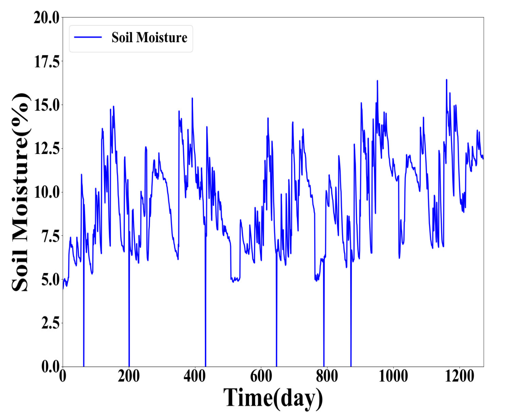
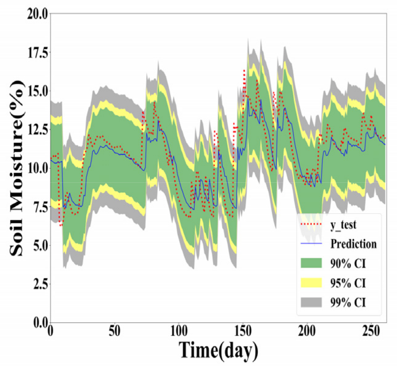
In this paper, the soil moisture data were collected during the period from 28 February 2012 to 8 November 2016, in Beijing, China. The collected original daily average soil moisture data were utilized to form the soil moisture time series as training and test datasets for analysis and prediction. The collected soil moisture data are plotted in Figure 1.

During the experiment, the 8 continuous historical soil moisture data points and its corresponding response points (the 9th, 10th, 11th data points) form a data item. In other words, the continuous soil moisture of 8 days is used to forecast the soil moisture in the following 3 days. The full dataset consists of 1272 data items. The first 1000 data items make up the complete training set, and the rest of the 272 data items form the test set.

Y(1), Y(2), and Y(3) indicate the daily average soil moisture of the 9th, 10th, 11th days, respectively. The full training dataset makes it very time-consuming to develop the GPR model, and thus the RU algorithm is applied to sample the representative dataset from the large full dataset. The sample sizes of 100 and 500 are considered for the sample selection to examine the performance of the proposed method. Finally, the GPR models built with the full training data and the chosen data separately are tested on the same test dataset.

3.2. Point Prediction Analysis

The prediction performance of the proposed model built with the full training data and the chosen training data in predicting Y(1), Y(2), and Y(3) are evaluated. Meanwhile, the published forecasting model based on ARMA algorithm [13] is considered as a benchmark. Four metrics, RMSE, MAE, MAPE, and time, are utilized to assess the forecasting performance, and experimental results are shown in

Table 1. Comparison of the proposed models built with two datasets in Y(1) prediction.

Model	RMSE	MAE	MAPE	Time(s)
GPR + full dataset	0.908	0.459	4.209	10.204
GPR + 100 data samples	0.878	0.446	4.092	0.339
GPR + 500 data samples	0.918	0.478	4.380	2.594
ARMA	0.920	0.590	5.626	1.058

Note: RMSE (root-mean-squared-error); MAE (mean absolute error); MAPE (mean absolute percentage error). Statistics in bold indicate best results.

,

Table 2. Comparison of the proposed models built with two datasets in Y(2) prediction.

Training Dataset Size	RMSE	MAE	MAPE	Time(s)
GPR + full dataset	1.267	0.792	7.255	14.795
GPR + 100 data samples	1.233	0.775	7.101	0.393
GPR + 500 data samples	1.280	0.816	7.480	3.833
ARMA	1.168	0.824	7.816	1.091

Statistics in bold indicate best results.

and

Table 3. Comparison of the proposed models built with two datasets in Y(3) prediction.

Training Dataset Size	RMSE	MAE	MAPE	Time(s)
GPR + full dataset	1.508	1.028	9.413	12.579
GPR + 100 data samples	1.457	0.970	8.886	0.324
GPR + 500 data samples	1.505	0.997	9.131	3.148
ARMA	1.636	1.271	9.880	1.119

Statistics in bold indicate best results.

. It can be seen from Table 1, Table 2 and Table 3 that the GPR model with the training sample sizes of 100 obtained the best performance over three models in terms of the lowest RMSE, MAE, and MAPE values. The GPR model trained using the 500 selected training samples yielded worse prediction results for Y(1) and Y(2) compared to the GPR model based on the full training dataset. However, the error difference is minor between these two models, and the forecasting performance of the GPR model trained using the 500 selected training samples is better for Y(3) prediction.

The point prediction results from Table 1, Table 2 and Table 3 show that using the chosen data can improve the prediction accuracy and much less computation time is required. Thanks to the RU design algorithm, the most representative subset is selected from the original training dataset. The better setting of the selected sample size can assist in improving the prediction performance of the GPR model and reducing the computation time simultaneously. Therefore, the proposed method is applicable for GPR point prediction using the large dataset. Compared with the ARMA-based model, the GPR model with the training sample sizes of 100 yields better forecasting performance in terms of lower RMSE, MAE, and MAPE values as well as shorter computing time.

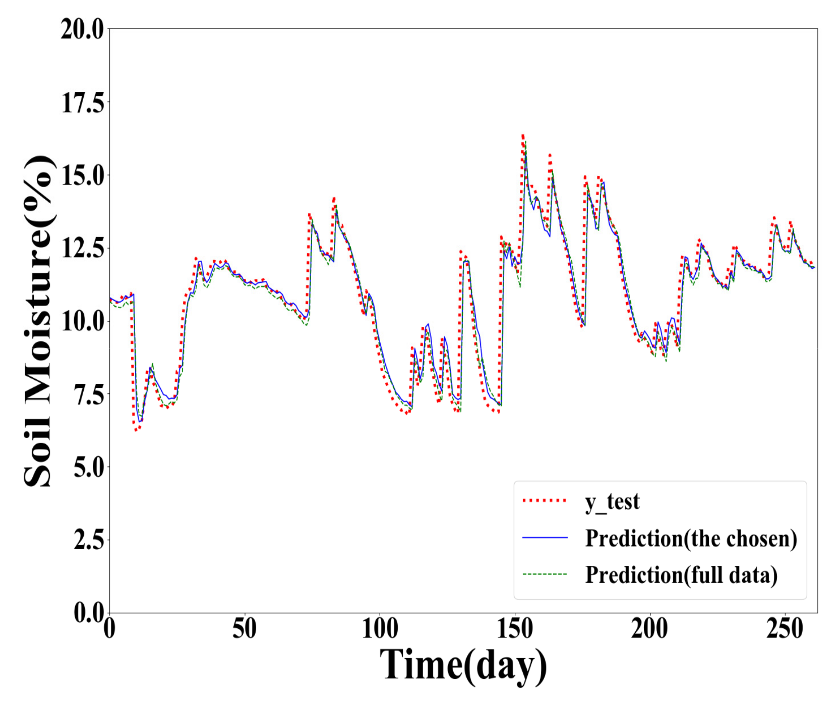
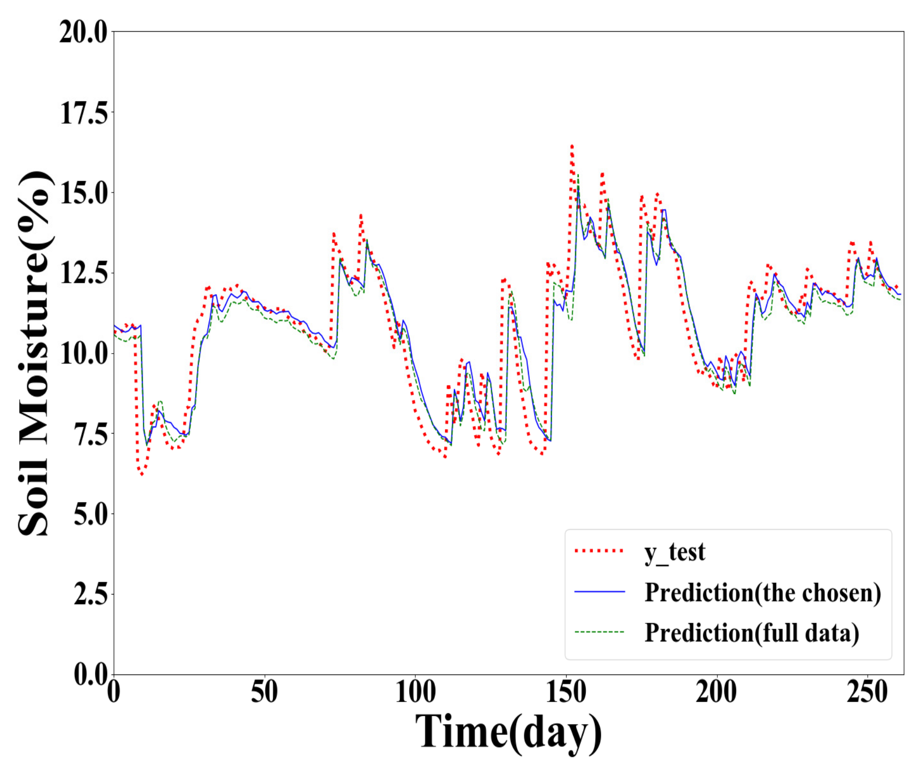
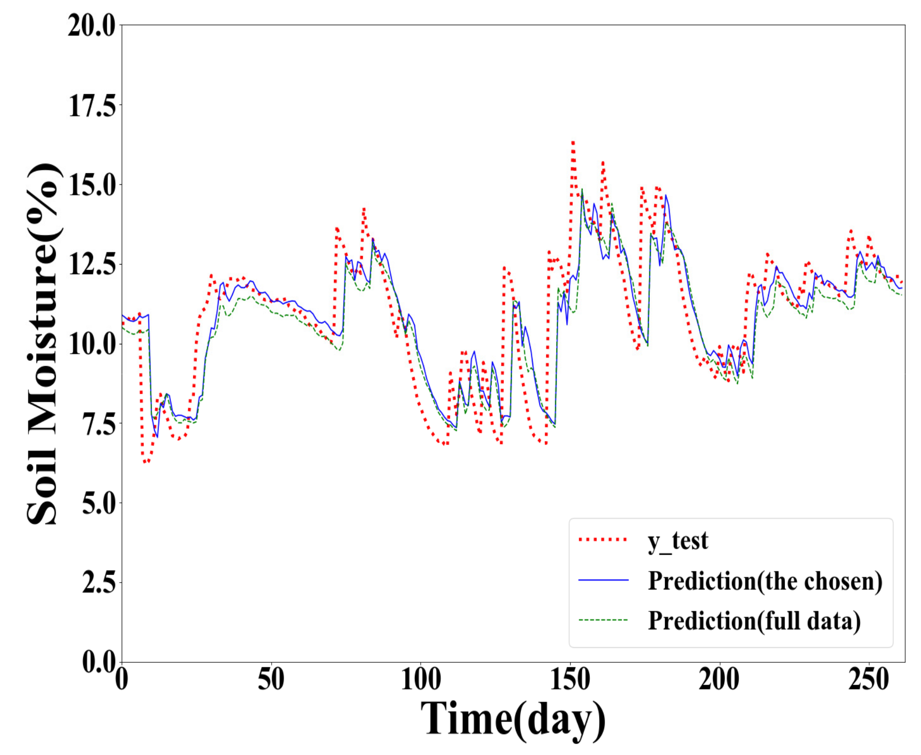
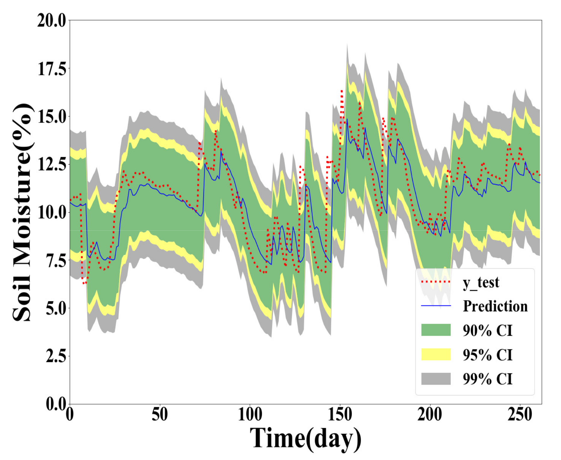
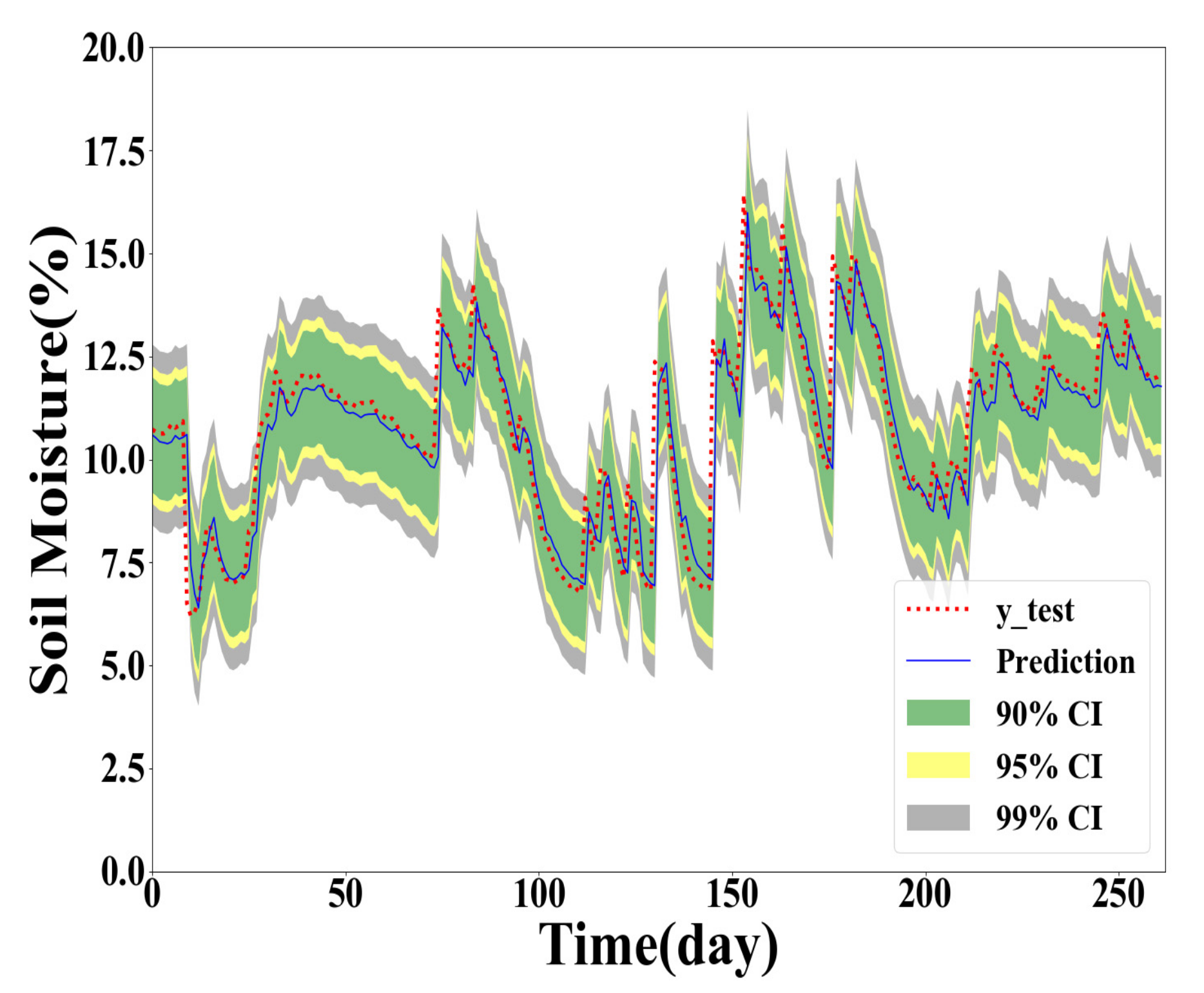
To further illustrate the performance of the proposed method, the results of the GPR models built with different training samples for Y(1), Y(2), and Y(3) prediction are plotted in Figure 2, Figure 3 and Figure 4. In point prediction, the 100 training samples were selected as the chosen data.

Compared with the prediction results shown in Figure 3 and Figure 4, the prediction results in Figure 2 are closer to the actual soil moisture. It indicates that the prediction accuracy decreases with the increasing of the forecasting horizon.

From Figure 2, Figure 3 and Figure 4, the red dotted line denotes the actual value curve, the blue line demonstrates the forecasting value curve of the GPR model trained in the chosen data whose size is 100, and the green intermittent line indicates the forecasting value curve of the GPR model trained in the full training dataset. It can be seen that the blue curve is closer to the red curve, showing that the prediction accuracy of the GPR model trained using the chosen training samples is higher than the GPR model based on the full training dataset.

3.3. Interval Prediction Result Analysis

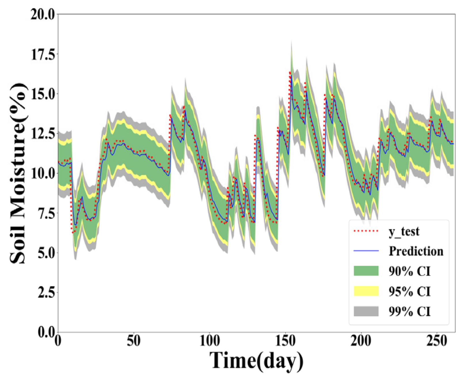
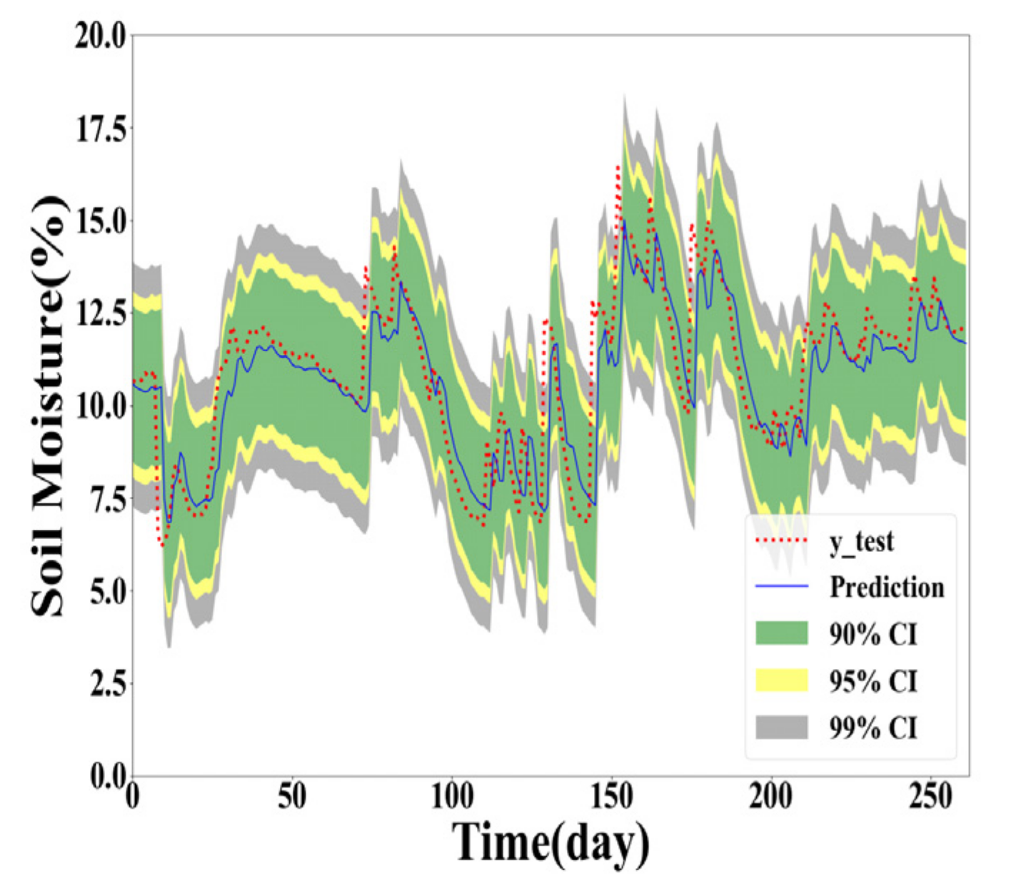
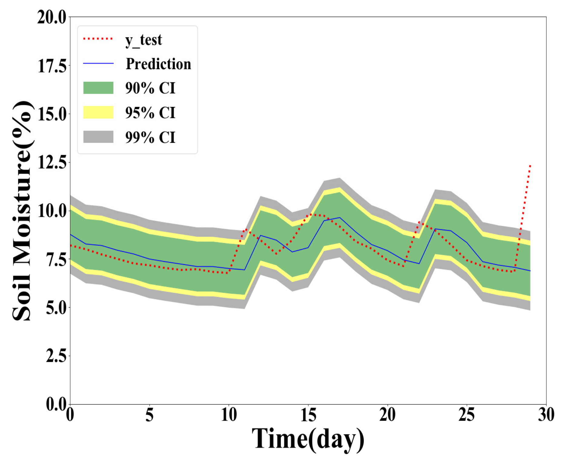
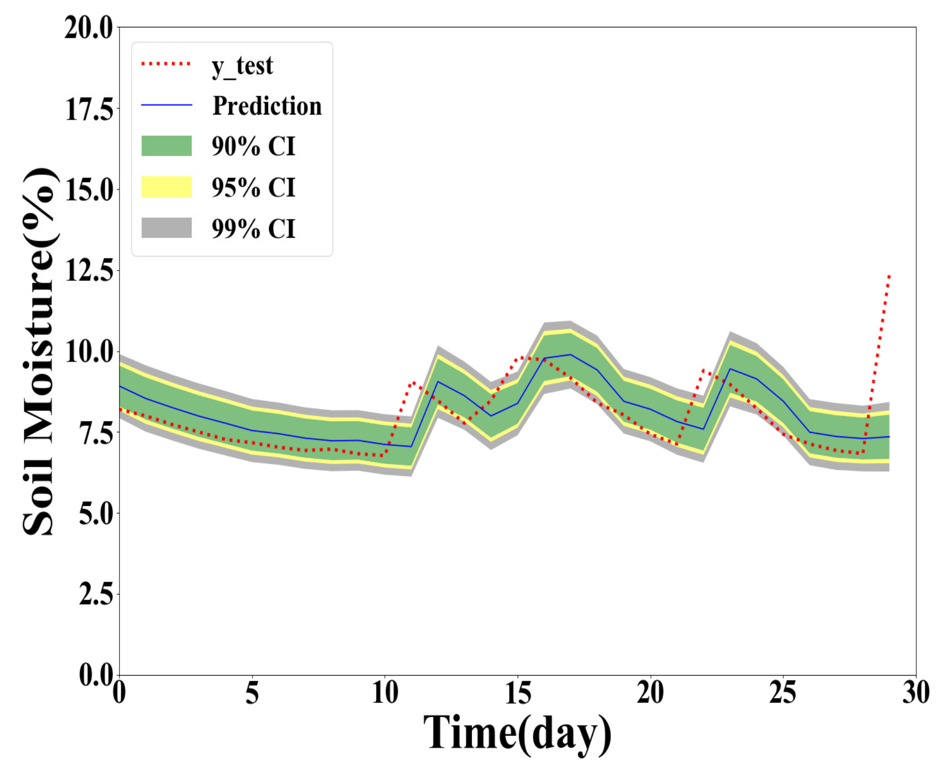
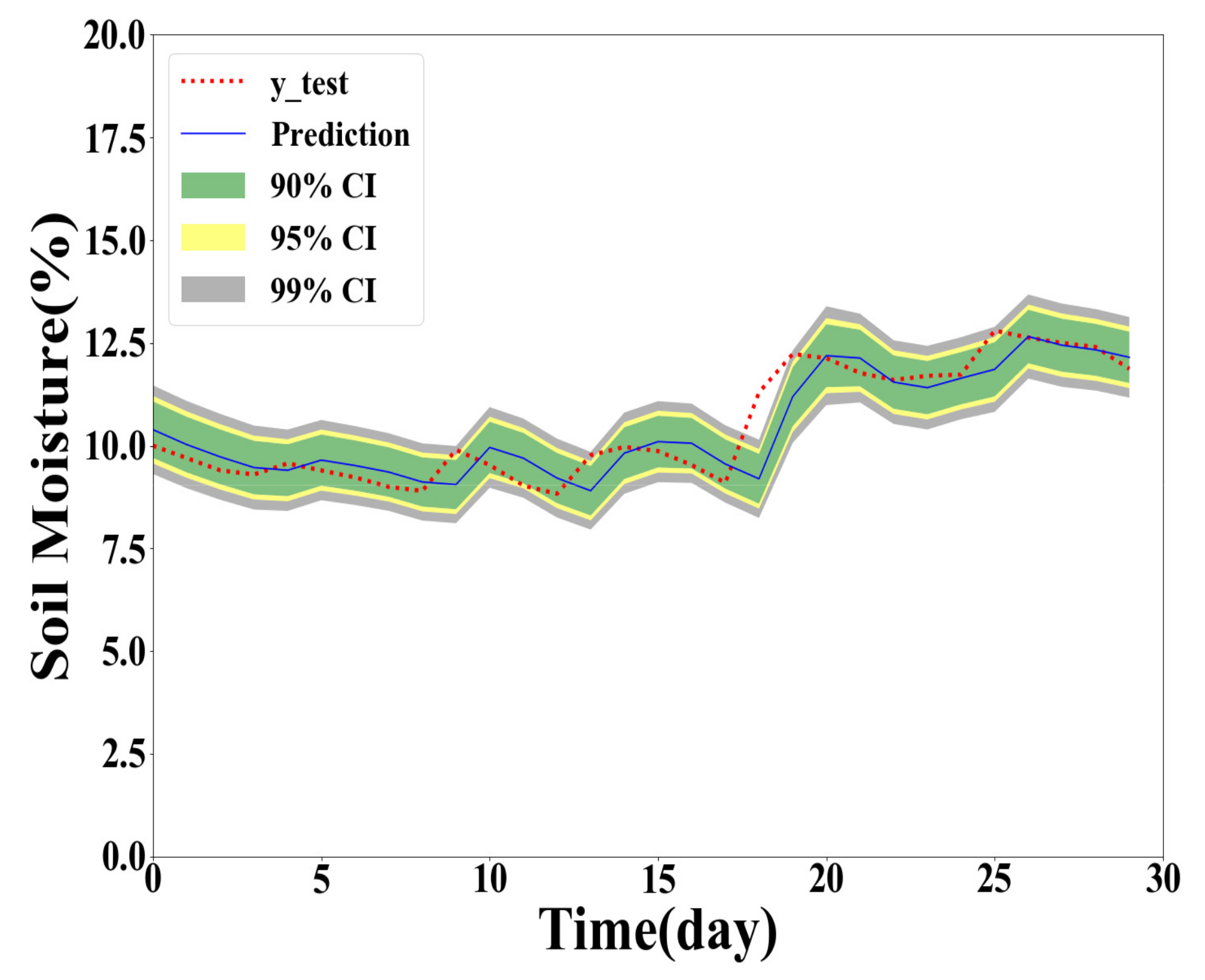
As shown in

Table 4. Evaluation results of PIs in Y(1) prediction.

PINC (%)	Training Dataset Size	PICP (%)	ACE (%)	Score
90	Full	93.130	3.130	−0.945
	100	83.969	−6.03	−0.889
95	500	93.129	3.129	−0.970
	Full	93.893	−1.107	−0.670
	100	87.786	−7.213	−0.702
	500	93.893	−1.106	−0.670
99	Full	95.802	−3.198	−0.340
	100	93.511	−5.488	−0.494
	500	96.564	−2.435	−0.321

Statistics in bold indicate best results.

,

Table 5. Evaluation results of PIs in Y(2) prediction.

PINC (%)	Training Dataset Size	PICP (%)	ACE (%)	Score
90	Full	92.366	2.366	−1.296
	100	85.496	−4.503	−1.262
95	500	93.129	3.129	−1.311
	Full	94.275	−0.725	−0.874
	100	89.312	−5.687	−0.921
	500	95.038	0.038	−0.870
99	Full	95.420	−3.580	−0.381
	100	93.511	−5.488	−0.519
	500	95.801	−3.198	−0.351

Statistics in bold indicate best results.

and

Table 6. Evaluation results of PIs in Y(3) prediction.

PINC (%)	Training Dataset Size	PICP (%)	ACE (%)	Score
90	Full	90.839	0.839	−1.518
	100	80.152	−9.847	−1.551
95	500	91.984	1.984	−1.507
	Full	92.748	−2.252	−0.975
	100	86.641	−8.358	−1.114
	500	92.748	−2.251	−0.960
99	Full	94.656	−4.344	−0.317
	100	91.221	−7.778	−0.603
	500	95.419	−3.580	−0.304

Statistics in bold indicate best results.

, the GPR model built with the training dataset size of 500 generally performs the best for Y(1), Y(2), and Y(3) prediction. However, the GPR model based on the full training dataset generates better PICP and ACE values for confidence level 90% in Y(2) and Y(3) prediction. The GPR model trained with the 100 samples obtained the worst interval prediction performance over the three models. A reasonable reason is that the GPR model cannot learn the true distribution well with fewer training data samples. To demonstrate the interval predication results, the PIs of the proposed method are provided in Figure 5, Figure 6, Figure 7 and Figure 8. In interval prediction, the 500 training samples are selected as the chosen data.

3.4. Discussion

In terms of point prediction, it can be seen from Table 1, Table 2 and Table 3 that the GPR model with the training sample sizes of 100 obtained the best performance based on the two datasets. Thus, the extracted subset training dataset includes the most representative training samples and the well-performed forecasting model is developed. Meanwhile, because only 100 data samples are utilized, two benefits can be observed: (1) since noise data is less likely to be sample, the forecasting accuracy can be improved; (2) the computational time is significantly reduced due to the small size of the kernel matrix. The GPR model trained using the 500 selected training samples yielded worse prediction results for Y(1) and Y(2) compared to the GPR model based on the full training dataset. However, regarding the Y(3) forecasting, the GPR model trained using the 500 selected training samples performed better than the latter model. A possible reason is that some noise points are included in the 500 samples, and thus the model performance degrades. Compared with the widely applied ARMA algorithm [16], the proposed model has achieved better performance. The execution time of the GRP model based on the 100 training samples is much less than that of the ARMA model. Therefore, the proposed model is more suitable for real-time forecasting applications.

For interval prediction, as shown in Table 4, Table 5 and Table 6, the GPR model built with the training dataset size of 500 generally performs the best for Y(1), Y(2), and Y(3) prediction. However, the GPR model based on the full training dataset generates better PICP and ACE values for confidence level 90% in Y(2) and Y(3) prediction. The GPR model trained with the 100 samples obtained the worst interval prediction performance over the three models. This phenomenon may occur because the GPR model cannot learn the true distribution well when the training data sample is small, and 500 sample points are enough for the model to learn the sample distribution, and the entire data set is not required. The interval prediction verifies the effectiveness of the RU design algorithm in selecting representative samples.

3.5. Seasonal Factor Analysis

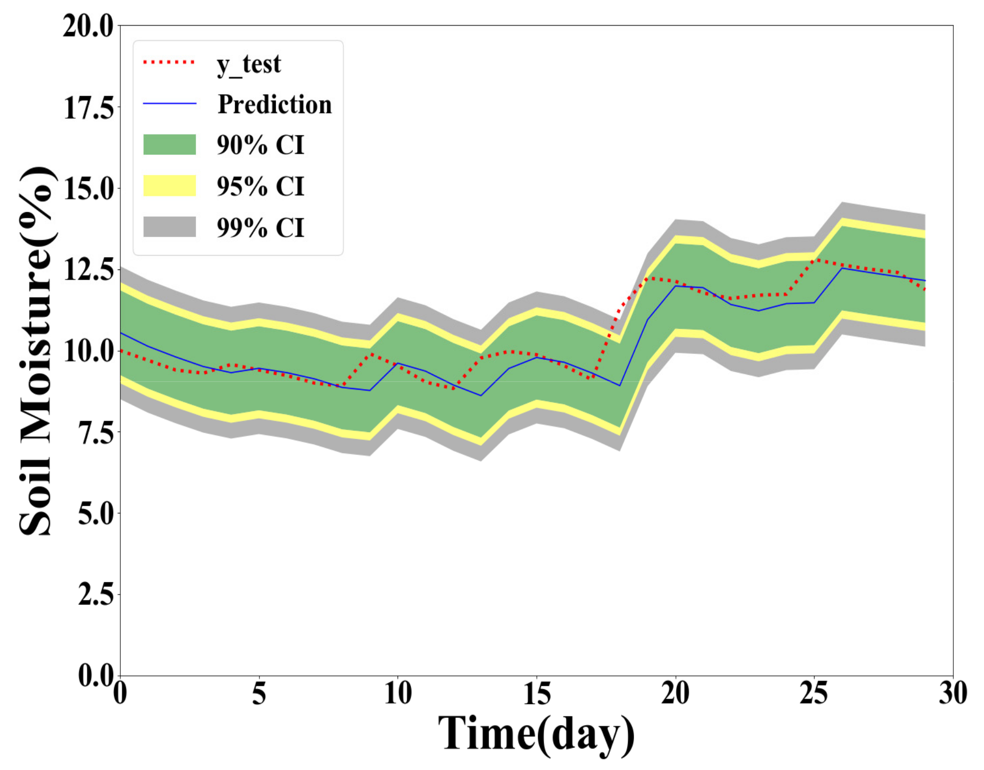
Taking the impact of the season factor on the forecasting performance into account, 30-day data of June (Summer) and September (Fall) was used as the test dataset respectively to compare the prediction performance based on different training sample size. The test data of June and September are noted as test June and test Sep.

From

Table 7. Y(1) Prediction of the proposed models built with full training dataset.

Test Dataset	RMSE	MAE	MAPE	Time(s)
full test	0.908	0.459	4.209	10.204
test June	1.253	0.719	8.940	10.686
test Sep	0.670	0.425	4.054	9.529

Statistics in bold indicate best results.

and

Table 8. Y(1) Prediction of the proposed models built with the chosen data whose size is 100.

Test Dataset	RMSE	MAE	MAPE	Time(s)
full test	0.878	0.446	4.092	0.339
test June	1.206	0.816	10.156	0.187
test Sep	0.584	0.414	3.947	0.207

Statistics in bold indicate best results.

, it is observed that the RMSE, MAE, MAPE values of the GPR models for test June are all higher than those of models for full test data. However, the performance of GPR models for test Sep is better than that of GPR models for full test data. The interval prediction results of the two selected months are drawn in Figure 8, Figure 9, Figure 10 and Figure 11.

It is demonstrated in Figure 11, Figure 12, Figure 13 and Figure 14 that the seasonal factor has an impact on the prediction performance of the GPR models. In June, the weather changes dramatically with much rainfall. Therefore, compared with September, the prediction in June is more difficult. It is more challenging to forecast soil moisture in summer.

4. Conclusions

In this paper, an RU design algorithm was applied to sample representative data points to develop the GPR model in predicting the soil moisture. The following conclusions are drawn from this study.

(1) Through the RU design algorithm, the most representative subset (the chosen data) was sampled from the complete training dataset. Based on the chosen data with proper sample size setting, the performance of the GPR model was improved and much less computing time was required.

(2) The RMSE, MAE, and MAPE values of the GPR model built with the chosen data were smaller compared with the GPR model based on the full training data in terms of the point prediction.

(3) Regarding the interval prediction, PIs of the GPR model built with the chosen data were better considering the reliability, sharpness and overall skill.

In future work, the integration of the RU design algorithm and other learning algorithms, such as deep neural networks [33] and boosted regression trees [34], will be investigated for the soil moisture prediction.

References

- Seneviratne, S.I.; Corti, T.; Davin, E.L.; Hirschi, M.; Jaeger, E.B.; Lehner, I.; Orlowsky, B.; Teuling, A.J. Investigating soil moisture–climate interactions in a changing climate: A review. Earth Sci. Rev. 2010, 99, 125–161. [Google Scholar] [CrossRef]
- Garg, A.; Gadi, V.K.; Feng, Y.C.; Lin, P.; Qinhua, W.; Ganesan, S.; Mei, G. Dynamics of soil water content using field monitoring and AI: A case study of a vegetated soil in an urban environment in China. Sustain. Comput. Inform. Syst. 2019, 100301. [Google Scholar] [CrossRef]
- Chatterjee, S.; Dey, N.; Sen, S. Soil moisture quantity prediction using optimized neural supported model for sustainable agricultural applications. Sustain. Comput. Inform. Syst. 2018. [Google Scholar] [CrossRef]
- Corradini, C. Soil moisture in the development of hydrological processes and its determination at different spatial scales. J. Hydrol. 2014, 516, 1–5. [Google Scholar] [CrossRef]
- Brocca, L.; Ciabatta, L.; Massari, C.; Camici, S.; Tarpanelli, A. Soil moisture for hydrological applications: Open questions and new opportunities. Water 2017, 9, 140. [Google Scholar] [CrossRef]
- Sehgal, V.; Venkataramana, S. Watershed-scale retrospective drought analysis and seasonal forecasting using multi-layer, high-resolution simulated soil moisture for Southeastern US. Weather Clim. Extrem. 2019, 23, 100191. [Google Scholar] [CrossRef]
- Ford, T.W.; Quiring, S.M. Comparison of contemporary in situ, model, and satellite remote sensing soil moisture with a focus on drought monitoring. Water Resour. Res. 2019, 55, 1565–1582. [Google Scholar] [CrossRef]
- Pendergrass, A.G.; Meehl, G.A.; Pulwarty, R.; Hobbins, M.; Hoell, A.; AghaKouchak, A.; Bonfils, C.J.; Gallant, A.J.; Hoerling, M.; Hoffmann, D.; et al. Flash droughts present a new challenge for subseasonal-to-seasonal prediction. Nat. Clim. Chang. 2020, 10, 191–199. [Google Scholar] [CrossRef]
- Brocca, L.; Melone, F.; Moramarco, T.; Wagner, W.; Naeimi, V.; Bartalis, Z.; Hasenauer, S. Improving runoff prediction through the assimilation of the ASCAT soil moisture product. Hydrol. Earth Syst. Sci. 2010, 14, 1881–1893. [Google Scholar] [CrossRef] [Green Version]
- Koster, R.D.; Mahanama, S.P.; Livneh, B.; Lettenmaier, D.P.; Reichle, R.H. Skill in streamflow forecasts derived from large-scale estimates of soil moisture and snow. Nat. Geosci. 2010, 3, 613. [Google Scholar] [CrossRef]
- Brocca, L.; Ponziani, F.; Moramarco, T.; Melone, F.; Berni, N.; Wagner, W. Improving landslide forecasting using ASCAT-derived soil moisture data: A case study of the Torgiovannetto landslide in central Italy. Remote Sens. 2012, 4, 1232–1244. [Google Scholar] [CrossRef] [Green Version]
- Bittelli, M.; Valentino, R.; Salvatorelli, F.; Pisa, P.R. Monitoring soil-water and displacement conditions leading to landslide occurrence in partially saturated clays. Geomorphology 2012, 173, 161–173. [Google Scholar] [CrossRef]
- Yang, S.; Yiming, W.; Zhengqin, G. Research on soil moisture forecast based on ARIMA model. Agric. Res. Arid Areas 2006, 24, 114–118. [Google Scholar]
- Chifflard, P.; Kranl, J.; Zur Strassen, G.; Zepp, H. The significance of soil moisture in forecasting characteristics of flood events. A statistical analysis in two nested catchments. J. Hydrol. Hydromech. 2018, 66, 1–11. [Google Scholar] [CrossRef] [Green Version]
- Graham, S.L.; Laubach, J.; Hunt, J.E.; Eger, A.; Carrick, S.; Whitehead, D. Predicting soil water balance for irrigated and non-irrigated lucerne on stony, alluvial soils. Agric. Water Manag. 2019, 226, 105790. [Google Scholar] [CrossRef]
- Chen, H. Research on Soil Moistrue Prediction Models of Inadequate Irrigation Rice Field in South China. Ph.D. Thesis, Yangzhou University, Yangzhou, China, 2004. [Google Scholar]
- Mahmood, R.; Hubbard, K.G. An analysis of simulated long-term soil moisture data for three land uses under contrasting hydroclimatic conditions in the Northern Great Plains. J. Hydrometeorol. 2004, 5, 160–179. [Google Scholar] [CrossRef] [Green Version]
- Liang-chen, Z. Study on Estimation of Soil-water Content by Using Soil-Water Dynamics Model. Water Sav. Irrig. 2007, 3, 10–13. [Google Scholar]
- Ines, A.V.; Das, N.N.; Hansen, J.W.; Njoku, E.G. Assimilation of remotely sensed soil moisture and vegetation with a crop simulation model for maize yield prediction. Remote Sens. Environ. 2013, 138, 149–164. [Google Scholar] [CrossRef] [Green Version]
- Zhang, X.; Tang, Q.; Liu, X.; Leng, G.; Li, Z. Soil moisture drought monitoring and forecasting using satellite and climate model data over southwestern China. J. Hydrometeorol. 2017, 18, 5–23. [Google Scholar] [CrossRef]
- Xiao-gang, M.A. Forecast of Soil Moisture Content during Critical Period of Spring Sowing Based on Precipitation in Last Autumn. Chin. J. Agrometeorol. 2008, 29, 55–57. [Google Scholar]
- Sukhwinder, S.; Kaur, S.; Kumar, P. Forecasting soil moisture based on evaluation of time series analysis. In Advances in Power and Control Engineering; Springer: Singapore, 2020; pp. 145–156. [Google Scholar]
- Prasad, R.; Deo, R.C.; Li, Y.; Maraseni, T. Soil moisture forecasting by a hybrid machine learning technique: ELM integrated with ensemble empirical mode decomposition. Geoderma 2018, 330, 136–161. [Google Scholar] [CrossRef]
- Huang, C.; Li, L.; Ren, S.; Zhou, Z. Research of soil moisture content forecast model based on genetic algorithm BP neural network. In International Conference on Computer and Computing Technologies in Agriculture; Springer: Berlin/Heidelberg, Germany, 2010. [Google Scholar]
- Yi, L.; Tao Chen, T.; Chen, J. Auto-switch Gaussian process regression-based probabilistic soft sensors for industrial multigrade processes with transitions. Ind. Eng. Chem. Res. 2015, 54, 5037–5047. [Google Scholar]
- Liu, Y.; Chou, C.P.; Chen, J.; Lai, J.Y. Active learning assisted strategy of constructing hybrid models in repetitive operations of membrane filtration processes: Using case of mixture of bentonite clay and sodium alginate. J. Membr. Sci. 2016, 515, 245–257. [Google Scholar] [CrossRef]
- Yi, L.; Wu, Q.-Y.; Chen, J. Active selection of informative data for sequential quality enhancement of soft sensor models with latent variables. Ind. Eng. Chem. Res. 2017, 56, 4804–4817. [Google Scholar]
- Huang, C.; Zhao, Z.; Wang, L.; Zhang, Z.; Luo, X. The Point and Interval Forecasting of Solar Irradiance with an Active Gaussian Process. IET Renew. Power Gener. 2020, 14, 1020–1030. [Google Scholar] [CrossRef]
- Long, W.; Zhang, Z. Automatic detection of wind turbine blade surface cracks based on UAV-taken images. IEEE Trans. Ind. Electron. 2017, 64, 7293–7303. [Google Scholar]
- Rasmussen, C.E. Gaussian processes in machine learning. In Summer School on Machine Learning; Springer: Berlin/Heidelberg, Germany, 2003. [Google Scholar]
- Matthias, T.; Zhang, Z. Wind turbine modeling with data-driven methods and radially uniform designs. IEEE Trans. Ind. Inform. 2016, 12, 1261–1269. [Google Scholar]
- Huang, C.; Zhao, Z.; Wang, L.; Zhang, Z.; Luo, X. A hybrid approach for probabilistic forecasting of electricity price. IEEE Trans. Smart Grid 2013, 5, 463–470. [Google Scholar]
- Wang, L.; Zhang, Z.; Long, H.; Xu, J.; Liu, R. Wind Turbine Gearbox Failure Identification with Deep Neural Networks. IEEE Trans. Ind. Inform. 2017, 13, 1360–1368. [Google Scholar] [CrossRef]
- Huang, C.; Wang, L.; Lai, L.L. Data-Driven Short-Term Solar Irradiance Forecasting Based on Information of Neighboring Sites. IEEE Trans. Ind. Electron. 2019, 66, 9918–9927. [Google Scholar] [CrossRef]
Figure 1.
Full data of daily average soil moisture.
Figure 2.
Points forecasting results in Y(1) prediction.
Figure 3.
Points forecasting results in Y(2) prediction.
Figure 4.
Points forecasting results in Y(3) prediction.
Figure 5.
GPR model built with full training data in Y(1) prediction.
Figure 6.
GPR model built with full training data in Y(2) prediction.
Figure 7.
GPR model built with full training data in Y(3) prediction.
Figure 8.
GPR model built with the chosen data in Y(1) prediction.
Figure 9.
GPR model built with the chosen data in Y(2) prediction.
Figure 10.
GPR model built with the chosen data in Y(3) prediction.
Figure 11.
Y(1) prediction with full training data and testing in test June.
Figure 12.
Y(1) prediction with the chosen training data and testing in test June.
Figure 13.
Y(1) prediction with full training data and testing in test Sep.
Figure 14.
Y(1) prediction with the chosen training data and testing in test Sep.