An Integrated Approach for Assessing Flood Risk in Historic City Centres


1
ISISE, Institute of Science and Innovation for Bio-Sustainability (IB-S), Department of Civil Engineering, University of Minho, 4800-058 Guimarães, Portugal
2
Centre for Geographical Studies, Institute of Geography and Spatial Planning, University of Lisbon, 1600-276 Lisbon, Portugal
*
Author to whom correspondence should be addressed.
Water 2020, 12(6), 1648; https://0-doi-org.brum.beds.ac.uk/10.3390/w12061648
Submission received: 9 May 2020
/
Revised: 2 June 2020
/
Accepted: 7 June 2020
/
Published: 9 June 2020
(This article belongs to the Special Issue Recent Advances in the Assessment of Flood Risk in Urban Areas)
Abstract
:Historic city centres near watercourses are a specific type of urban area that are particularly vulnerable to flooding. In this study, we present a new methodology of flood risk assessment that crosses hazard and physical vulnerability information. We have selected the Historic City Centre of Guimarães (Portugal), a UNESCO Heritage Site, for developing and testing the defined methodology. The flood hazard scenario was obtained through the hydrologic–hydraulic modelling of peak flows with a 100-year return period, which provided flood extent, depths, and velocities. A decomposition of the momentum equation, using depth and velocity, allowed reaching a final hazard score. Flood vulnerability was assessed through combining an exposure component and a sensitivity component, from field-collected data regarding wall orientation, heritage status, age, number of storeys, condition, and material of buildings. By combining the results of the hazard and vulnerability modules in a risk-matrix, three qualitative levels of flood risk were defined. The individual and crossed analysis of results proved to be complementary. On one hand, it allows the identification of the more relevant risk factors—from the hazard or vulnerability modules. On the other hand, the risk-matrix identified other buildings with a high risk that otherwise would remain unnoticed to risk managers.
1. Introduction
The dizzying rate of urbanisation over the last few decades has led to an exponential increase in the magnitude of losses caused by natural and technological hazards worldwide. According to the risk-related literature, these losses can be understood as the consequence of a certain level of risk associated with a specific community or society over some specified time period [1]. In a broader sense, disaster risk is a compound concept determined by the combination of the hazard, exposure, and intrinsic vulnerability. Moreover, because vulnerability and hazard may change over time, disaster risk is highly dynamic [2,3]. For this reason, it is fundamental to have ways of monitoring this risk and, when necessary, supporting the definition and implementation of risk mitigation actions.
As a result of their heritage value and high physical vulnerability, historical centres are particularly critical areas and, therefore, deserve particular attention. According to the literature [4,5], in the last few decades, the impact of flooding events in historic centres has indeed increased steadily. As reported by Miranda and Ferreira [6], examples of recent high-impacting flooding events in historical centres include those that occurred in Central Europe, back in 2002 and 2010, in South Asia, in 2007 and 2008, and the New Orleans flood of 2005, caused by Hurricane Katrina. In a recent attempt to study this phenomenon, Marzeion and Levermann [7] investigated the number of cultural heritage sites worldwide that, due to global warming, are at risk of being flooded in the next two millennia. The results of this study are quite conclusive, pointing out that approximately 6% of current UNESCO sites (about 40 sites) will be flooded, particularly in China and India.
The present article addresses this challenge by discussing the application of an integrated flood risk assessment approach, which combines flood hazard and building vulnerability indicators to identify and classify risk and to narrow intervention priorities. The Historic City Centre of Guimarães (Portugal)—a World Heritage Site inscribed by UNESCO since 2001 due to its extraordinary authenticity and well-preserved condition—is explored here to illustrate the application of the methodology. After modelling the flood hazard using the hydrologic–hydraulic method and evaluating the flood vulnerability of the buildings by resorting to a simplified vulnerability assessment method, we provide a comprehensive analysis of the outputs, both in an individual and integrated manner. Finally, we used a risk-matrix approach to aggregate these hazard and vulnerability outputs and categorise the buildings into three qualitative levels of risk.
More than the results themselves—which are indeed very important for the Municipality of Guimarães, but eventually will be of little relevance to the reader—the interest and the innovation of this paper lies in how this integrated flood risk assessment approach (which results from the original combination of two already existing methods) can be used to individualise and guide intervention decisions. It is this analysis that, we believe, can be of great interest and direct relevance to the reader’s own practice.
2. The Historic City Centre of Guimarães
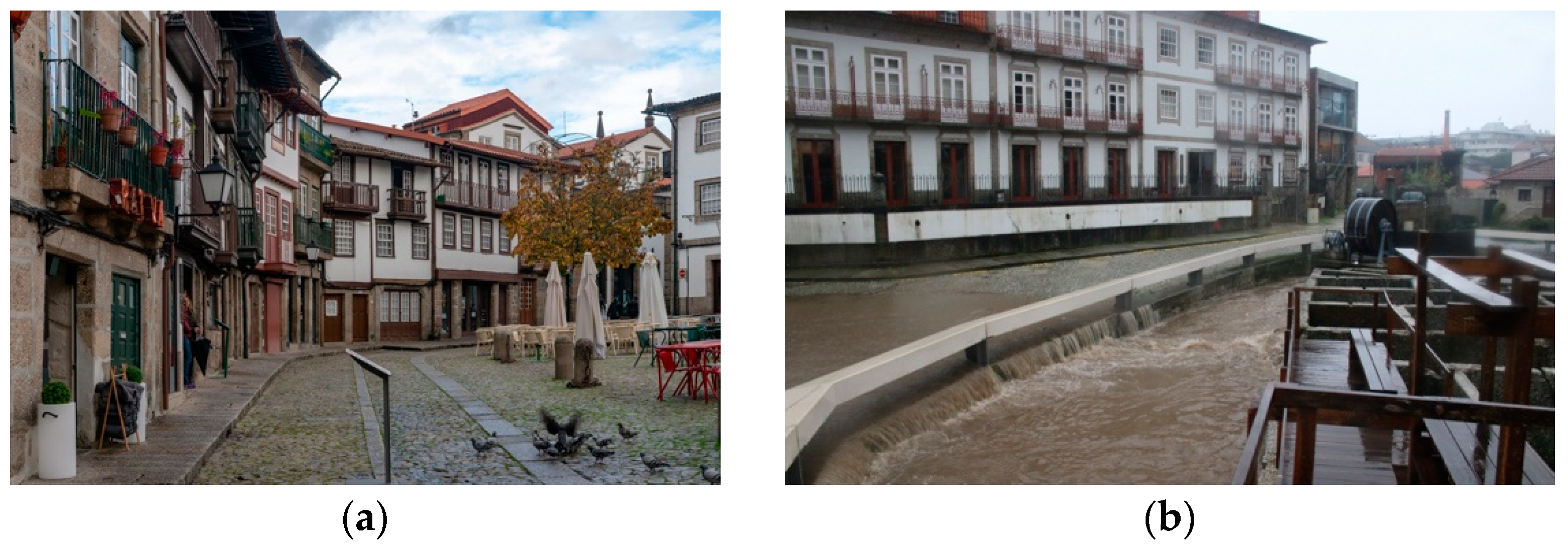
Located in northern Portugal, the city of Guimarães is usually referred to as the cradle of the Portuguese nationality [8]. The Historic City Centre of Guimarães is a World Heritage Site, deemed as such in 2001. According to the classification committee, the Historic City Centre of Guimarães is an exceptionally well-preserved and authentic example of the evolution of a Medieval settlement into a modern town, see Figure 1a. The architectural characteristics of the Historic City Centre of Guimarães, marked by a rich diversity of construction typologies associated with different evolution periods of the place, as well as its unity and integration with the landscape setting, compounds outstanding universal values.
According to Miranda and Ferreira [6], in recent decades, the city of Guimarães has been subjected to intense anthropogenic pressure as a result of a steady increase of urban and industrial occupation. This has led to the depreciation of the Couros river basin, which was once a central part of the population’s life and a vital element for the development of the leather industry [9]. As a result, the levels of pollution and contamination in the Couros creek, as well as the severity of flood events in the Historic City Centre of Guimarães, have increased substantially, Figure 1b.
The coexistence of the aspects mentioned above makes the assessment of the flood risk in the Historic City Centre of Guimarães a particularly challenging and relevant work, constituting, therefore, the justification for the selection of this case study.
Past Flood Events in the Historic City Centre of Guimarães
The Couros river basin (11.2 km2) is part of the Selho river basin (67.7 km2), which is a sub-basin of the Ave river basin (1390 km2) which drains to the Atlantic Ocean. The Couros river (5.6 km length) is thus a small left tributary of Selho river, located entirely in the Municipality of Guimarães.
Water availability soon became a relevant driver of human occupancy along the Couros river valley that crosses the Historic City Centre of Guimarães.
According to the DISASTER database [10], there are 10 flood occurrences in the municipality. This database covers the period from 1865 to 2015 and includes only the most severe cases of flooding (i.e., when at least one casualty, injured, missing, displaced, or evacuated person is registered in the data sources). In the study area, along the Couros river, there are two flood occurrences of the DISASTER type, both occurring during the flood event of 28 February 1978: in the elder residential structure “Lar dos Santos Passos”, where 23 persons were evacuated; and a few hundred meters downstream, at the trucking station, where three families were evacuated.
Despite this apparently modest record of severe losses, the dense artificialisation and imperviousness of the basin—particularly in the Historic City Centre—has been causing frequent episodes of flooding with only material consequences and economic losses. The most recent occurred on 20 December 2019, which was associated with the Elsa atmospheric depression.
3. Materials and Methods
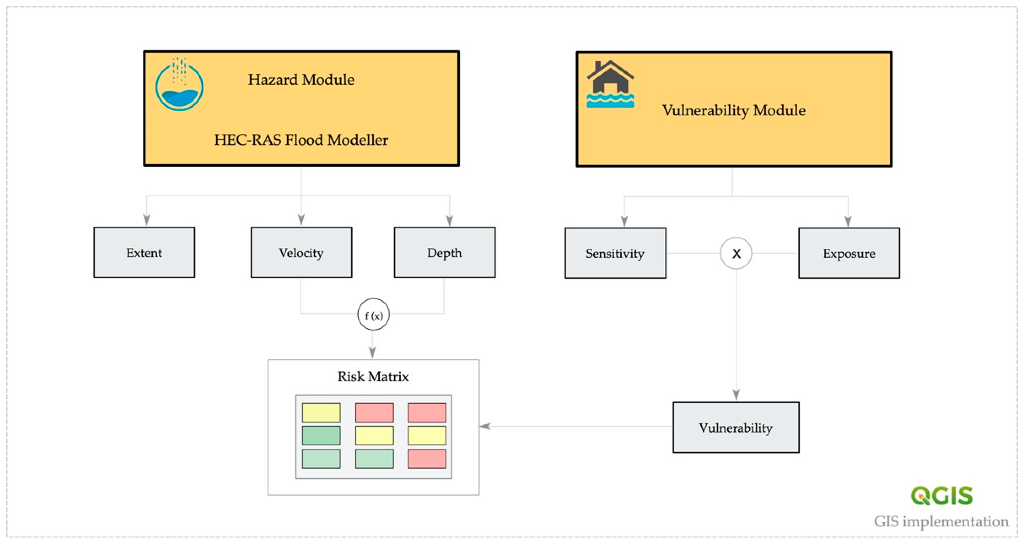
To better explain the methodological framework adopted in this work, this section presents and discusses the fundamentals of the applied flood risk assessment method. As schematically illustrated in Figure 2, the approach is composed of two main modules, the hazard and the vulnerability module. The bases of these two modules are detailed in Section 3.1 and Section 3.2. Finally, Section 3.4 introduces the study area and the approach adopted in this research to collect, manage, and explore data.
3.1. Hazard Module
The flood hazard was assessed using the hydrologic–hydraulic method. The assessment process involved the acquisition and preparation of geometric data, the estimation of the peak flow, the hydraulic modelling, and the GIS post-processing and mapping.
In the first step, we obtained the geometric data, representing the morphological features of the floodplain from a base map at a scale of 1:1000, contour lines 1 m equidistant, and a dense cover of mass points. Such data allowed us to create a detailed digital elevation model (DEM) with 1 m cell size, covering the entire valley of the Couros river, oriented E-W and crossing the Historic City Centre of Guimarães, illustrating how significantly modified by human intervention the natural morphology of the study area has been. The DEM features a topographic obstruction crossing the floodplain– and the Couros river—with an orientation N-S. At this section, flow occurs through a hydraulic passage of 30 m length, with a rectangular shape of 4.0 m 3.5 m, which was geometric and hydraulically modelled as a bridge. Roughness was represented through the Manning’s n value: 0.025 in the channel and 0.05 in overbank areas.
Flow data were estimated for the 100-year flood, based on the results obtained from the hydrologic study of Ramísio, Duarte, and Vieira [11,12], in which peak flows were obtained using empirical, kinematic, and statistical methods. The adopted 100-year peak flow results from a simple average of the estimates presented in the cited study, regarding four methods. Three of the methods are kinematic: the Giandotti, the rational method (using Kirpich concentration-time), and the rational method (using the Chow concentration-time). As for the rational method, we used the rainfall Intensity-Duration-Frequency (IDF) curve parameters from a rain gauge station located 45 km ENE of the study area, with a time series of 25 years. Although the gauge is located 45 km from the study area, it represents the same climatological and pluviogenic context found at the Couros river basin. Although the rain gauge is located at an elevation of 95 m, its 10 km radius has a mean elevation of 331.4 m, which is circa 70 m above the mean basin’s elevation of 258.8 m. Considering the mountainous context where both areas are located, such a difference can be considered as not relevant. Of the several rainfall durations for which those parameters are valid, we have adopted the interval 30 min to 6 h, which frames the concentration-time found in the upstream sub-basin that drains to the modelled reach—30.8 min and 71.7 min according to the Kirpich and Chow formulas, respectively. The rainfall duration is assumed to equal the concentration-time obtained from the simple average of the applied methods. The runoff coefficient C was estimated from the slope angle, land use data, and the degree of imperviousness [11]: 0.56 in the upstream basin and 0.73 in the basin crossed by the modelled stream of the Couros river.
The fourth method is a statistical one, designated as the Loureiro’s formula. This method uses the area of the basin and regional parameters, valid for the Portuguese context only, calculated from peak flow data fitted to the Gumbel distribution. The average of the four estimations was used from the Ramísio, Duarte, and Vieira [12] study in two sections: one, defined at the upstream inlet (35.95 m3/s, corresponding to a contributing basin of 3.75 km2); the other, estimated at the downstream outlet of the modelled reach (54.15 m3/s), the difference (18.2 m3/s) of which we have distributed along the 1786 m length of the modelled reach, proportionally to the drainage area of 11 pour points, Table 1.
By adopting this approach, we have intended to consider the effect of the complex sewer system that drains the small urban basins directly to the Couros river along the modelled reach.
Pre-processing of geometric data was performed at the HEC-RAS 5.0.7 environment [13], using the RAS Mapper tool. The modelled reach goes further downstream from the area to which the vulnerability of buildings was available. This is explained by the existence of the mentioned obstruction near the study area, leading us to model a flood pathway long enough to allow a proper elongation of floodwaters downstream of the obstruction. A normal depth slope of 0.015 m/m was used to define the downstream reach boundary conditions. A steady flow water surface computation was initiated at the upstream boundary using the 35.95 m3/s peak flow, to which the mentioned 11 flow change locations were sequentially added. In the modelling plan, we selected a mixed flow regime and requested the optional floodplain mapping.
Finally, we sequentially exported the HEC-RAS modelling results to SDF, XML, and GIS formats. Velocity and depth data were exported as GRID files (ESRI raster format) and the flood boundary as shapefile (vector polygon), both for the 100-year flood.
3.2. Vulnerability Module
Flood vulnerability is assessed through the application of the simplified flood vulnerability assessment methodology, which was initially proposed by Miranda and Ferreira [6]. This methodology consists of the evaluation of two vulnerability components, an exposure and a sensitivity component (Figure 2), which, through an index, quantify the vulnerability of the building to flood inundation.
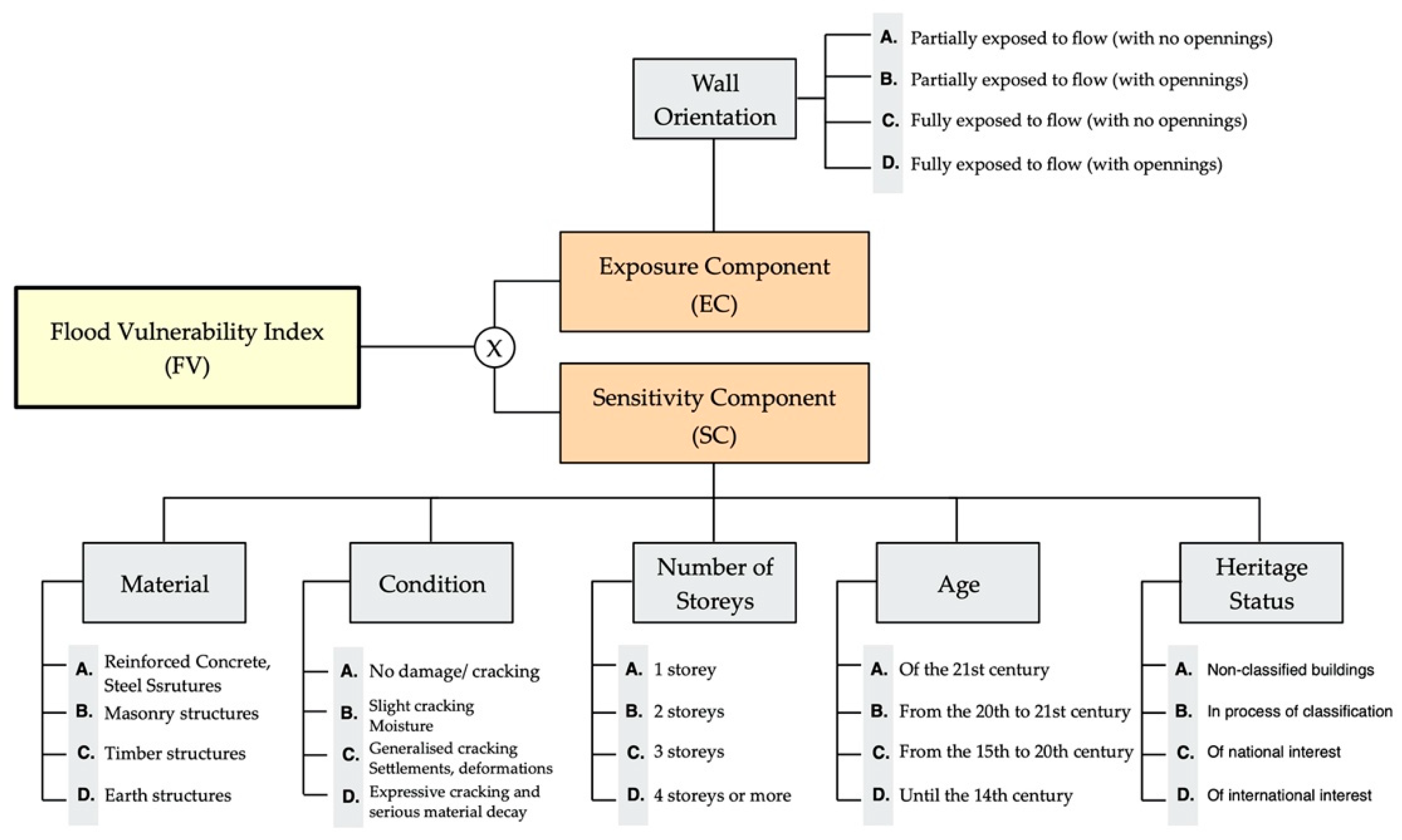
As presented in Figure 3, the Exposure Component is composed of one single parameter (Wall Orientation), which evaluates the influence of the orientation of the main façade wall of the building to the water flow. This parameter intends to bring together the multiple aspects behind this phenomenon: the location of the building, the orientation of its main façade wall, and the existence of openings, knowing that buildings located in low-lying areas are theoretically more susceptible to inundation due to runoff. Regarding the Sensitivity Component, this focusses on the physical characteristics of the building by evaluating its Material characteristics, Condition (or conservation state), Number of Storeys, Age, and Heritage Status. It is worth noting that these indicators were defined from a comprehensive review of analogous indicators proposed for assessing similar building typologies and structural characteristics under similar conditions [6].
We obtained the values of the exposure (EC) and the sensitivity (SC) components, which was done based on the vulnerability classes identified in Figure 3 (where A = 10, B = 40, C = 70, and D = 100), and individual flood vulnerability (FV) can be obtained using Equation (1).
For simplicity’s sake, the values of these three indices (EC, SC, and FV)—which range, respectively, from 10 to 100, 50 to 500, and 500 to 50,000—are normalised to fall within the range of 0 to 100; the lower the value of the index, the lower the level of exposure, sensitivity, or vulnerability of the building. According to Miranda and Ferreira [6], despite the fact that this approach was primarily intended for assessing the flood vulnerability of single buildings, its simple formulation makes it particularly suitable to evaluate large urban areas, such as historic city centres. It is precisely in this context that we apply this methodology herein.
3.3. Risk Matrix
Finally, flood risk is computed from the combination of the hazard and vulnerability results obtained by using the above-presented approaches. This is done through a vulnerability–hazard matrix, which relates each building’s vulnerability with the level of hazard to which it is exposed (see Table 2).
Regarding the vulnerability level, this is measured directly by the flood vulnerability index. For such, 20 and 40 were conservatively defined here as plausible threshold values for “moderate” and “high” vulnerability, respectively. Although this criterion may be debatable, it is important to note that the value of 40 (the boundary value between “moderate” and “high”) is frequently used in index-based vulnerability assessment approaches as a threshold for high vulnerability, see, for example, [14]. Concerning the level of hazard, this is obtained by combining flood velocity () and water depth () results according to the criterion given in Equation (2):
3.4. Study Area, Building Assessment, and Implementation of a Geographic Information System (GIS) Tool
The study area includes nine blocks with 116 buildings in total. Each one of these buildings was comprehensively assessed onsite to collect the data required for applying the flood vulnerability assessment approach, by using a detailed checklist. After being digitalised and systematised, the data that were contained in the checklists were manually inputted into a spreadsheet database to create a digital record and to automate some later steps of the work.
Once all the indices and flood indicators were computed, the results were plotted and analysed spatially using the open-source Geographic Information System software QGIS [17]. Geo-referenced graphical data (i.e., vectorised information and orthophoto maps) and specific information related to the hazard and the characteristics of the buildings were combined within the software to obtain first- and second-order outputs. In this case, each polygon (corresponding to a building) is associated with several features and attributes, allowing for their visualisation, selection, and search.
Because this GIS tool can efficiently combine highly-relevant hazard, vulnerability, and risk outputs in a very flexible and dynamic environment (easily updatable or modified at any time), it is undoubtedly a significant asset for risk management purposes, allowing the local authorities to define more consequent risk mitigation strategies.
4. Results and Discussion
Before getting into the integrated risk assessment outputs in Section 4.3, it is worth exploring the individual hazard and vulnerability results (in Section 4.1 and Section 4.2, respectively), which we define as first-order results.
4.1. Hazard Modelling
The flood modelling process described in Section 3.1 allowed us to obtain a broad set of primary hazard indicators, which, alone, give us good insight into the potential magnitude of a flood event in the study area. As already noticed in Section 3, we focused on three primary hazard indicators: flood extent, velocity, and water depth.
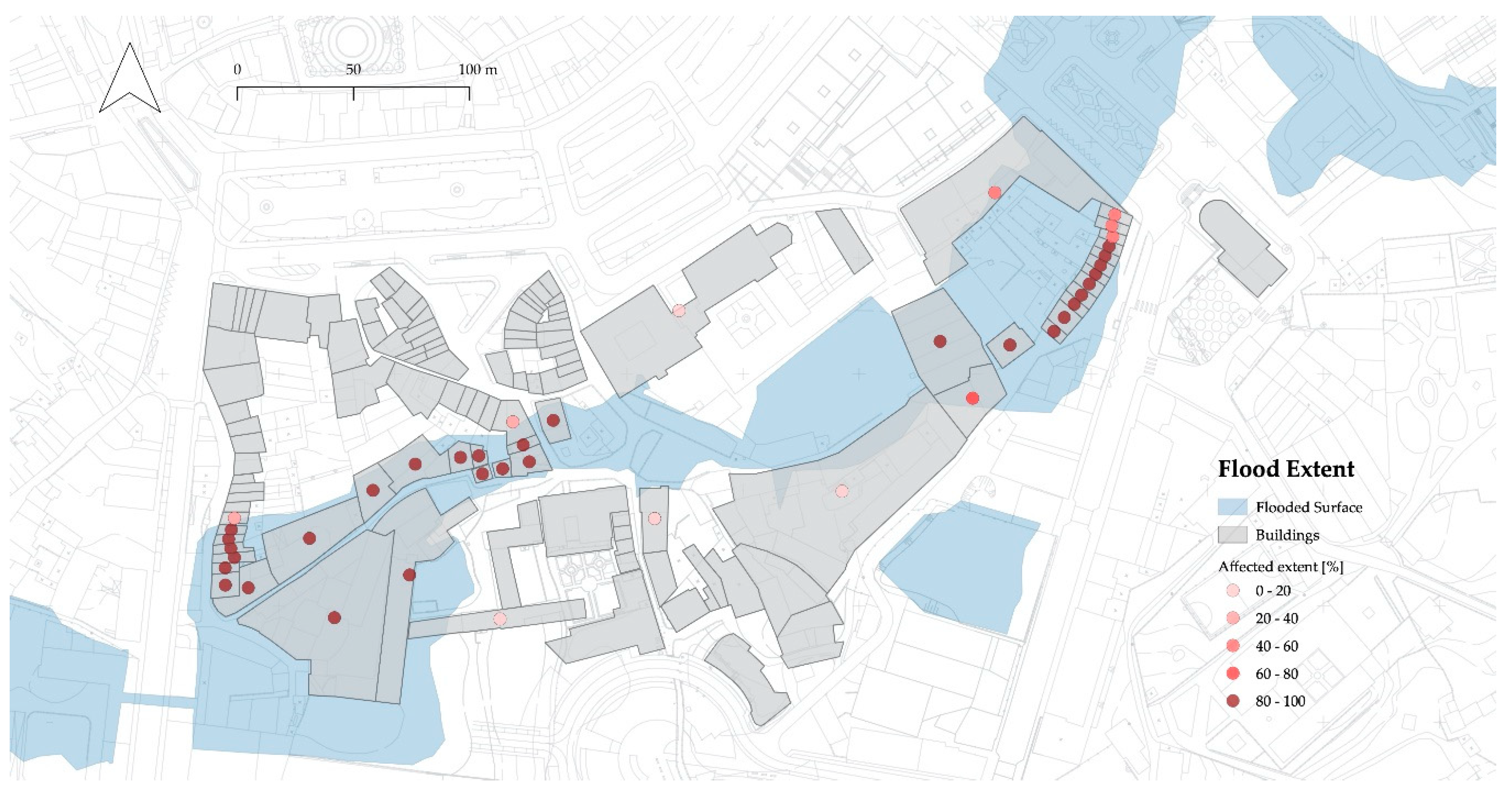
As for the flood extent, we found that for the adopted 100-year peak flow scenario, the study area was significantly affected by the flood. As illustrated in Figure 4, 41 out of the 116 buildings considered in this analysis are potentially affected by the flood.
Of these 41 buildings, 23 are affected to the fullest extent, whereas the other 18 are partially flooded, see Table 3. In absolute numbers, about 11,000 m2 of a total of about 32,000 m2 of built-up area are affected, which corresponds to about 34%.
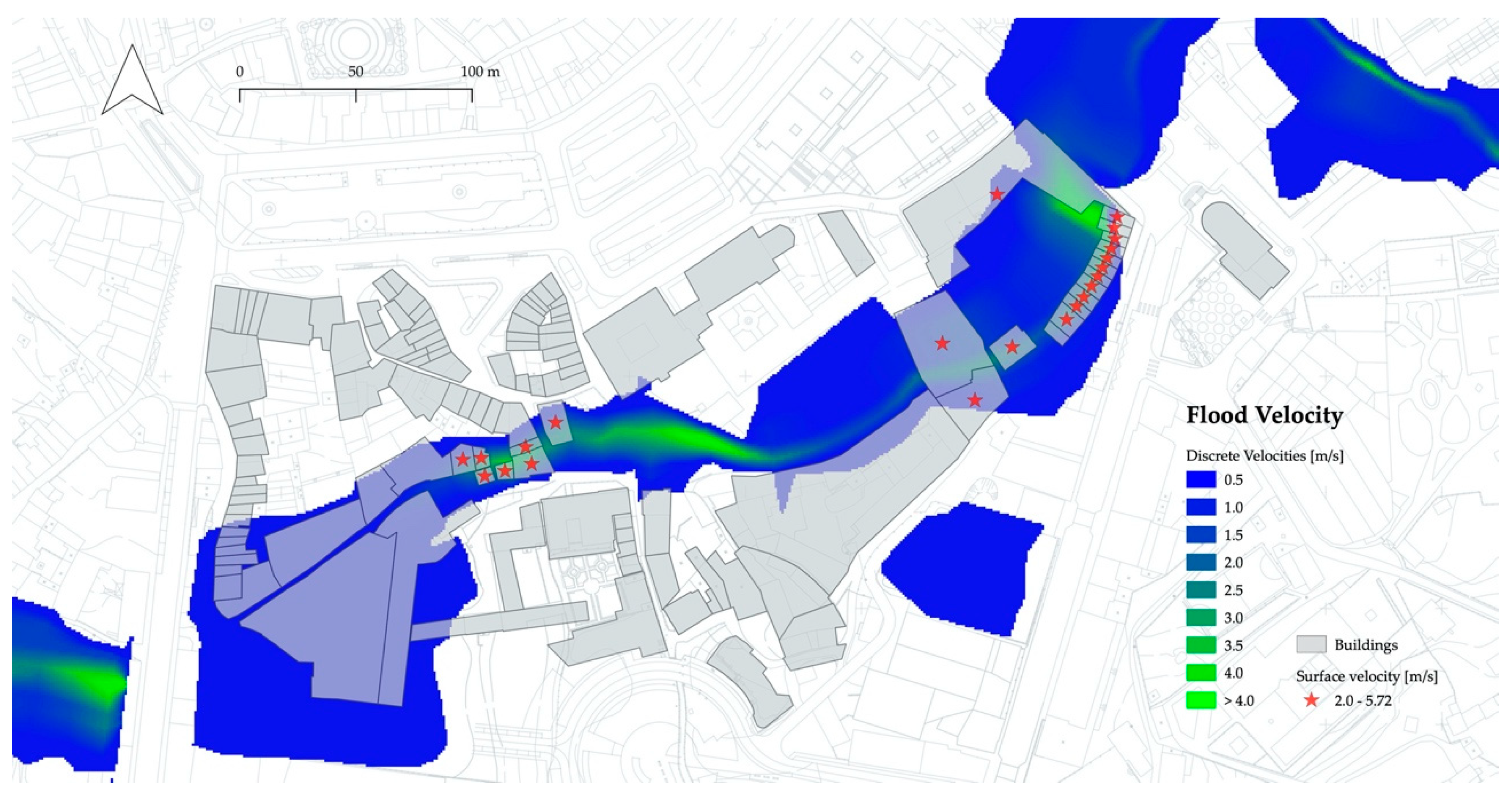
Concerning the flood velocity, presented in Figure 5, it ranges between 0.01 m/s and 5.72 m/s. The average velocity value at the surface of the 41 buildings affected by the flood is about 2.15 m/s—with a standard deviation value (STD) of 1.68—being that 22 of these 41 building are exposed to surface velocities higher than 2 m/s. As can be observed in Figure 5, there are two blocks that are particularly affected: one located in the northeast zone (15 buildings) and the other roughly at the central zone of the study area (7 buildings).
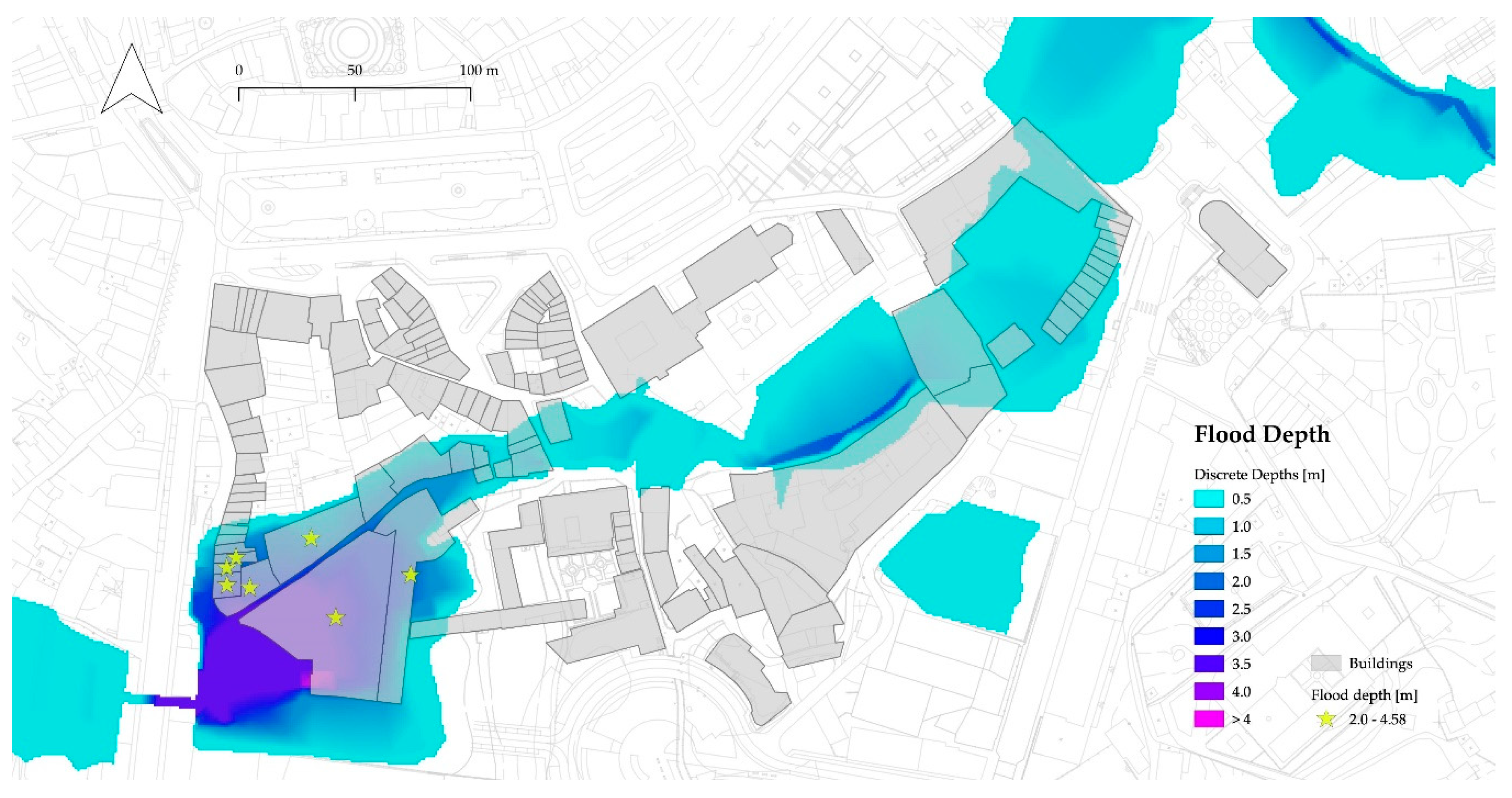
As for the water depth, from our hazard analysis, it was found that for the considered 100-year peak flow scenario, the buildings will expectably be exposed to an average depth of about 1.20 m (STD = 0.97). As illustrated in Figure 6, 31 out of the 41 buildings affected—which is slightly more than 75%—present a water height of more than 0.5 m, which is a very significant value. The maximum water depth value was obtained at the triangular shape building located at the southwest zone of the study area (4.58 m), see Figure 6.
Table 4 summarises the above-discussed results, presenting the absolute and relative number of potentially affected buildings for different ranges of flood velocity and water depth.
4.2. Flood Vulnerability
From the application of the flood vulnerability assessment approach detailed in Section 3.2, we found that 60% of the 116 buildings evaluated present a flood vulnerability value (FV) between 0 and 30. As presented in Figure 7, the remaining 40% present values ranging between 30 and 100. Statistically, the dataset has an average value of 25.70 (STD = 15.95).
Although flood damages cannot be estimated directly from these vulnerability values, the distribution shown in Figure 7 seems to demonstrate that a significant proportion of the buildings assessed are potentially very vulnerable to a flood event. We will provide more insight into this in Section 4.3.
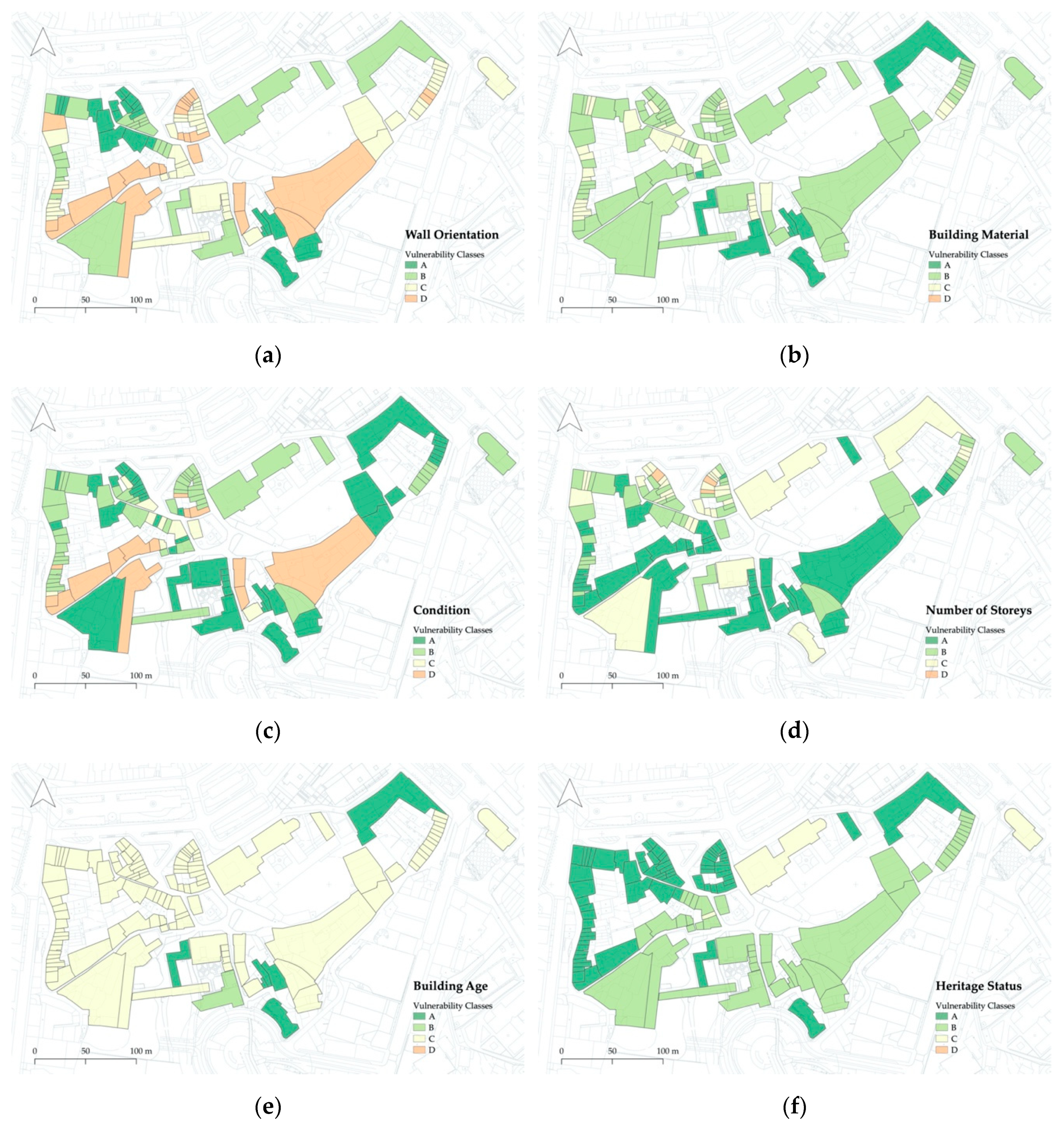
When exploring vulnerability results, it is often relevant to dive into the analysis of the specific parameters of the methodology. Such analysis allows for a better understanding of the vulnerability sources, which is a fundamental prerequisite to defining more consequent and effective risk mitigation measures. Figure 6 presents a set of six maps associated with the spatial distribution of the parameters that compose the flood vulnerability index.
A comprehensive discussion of the maps gathered in Figure 7 would be of little interest. However, we find it relevant to highlight some main results.
Firstly, the general conservation state of the buildings: As it is apparent in Figure 7c, in general, the buildings are either in good condition (Vulnerability Class A, 34%) or have minor conservation issues (Class B, 46%). Most of these minor conservation issues are related to small cracks or coating decay. Further, 20% of the buildings are in poor condition, presenting a significant cracking and moisture phenomena.
Secondly, the distribution of the number of storeys, in Figure 7d: This aspect is especially relevant since, according to several authors [18,19], the number of storeys has a direct influence on the vulnerability of the building to flooding. We will go into further detail regarding this when discussing the second-order risk results. For now, let us emphasise that 113 out of the 116 buildings evaluated have between 1 and 3 floors, distributed as follows: 38% are single-storey buildings, 33% have two storeys, and 27% have three.
Finally, the Heritage Status, in Figure 7f: This is a relevant aspect in the sense that buildings with heritage value deserve particular attention when it comes to risk assessment. Thus, regarding this aspect, 59% of the buildings assessed are ordinary buildings (i.e., non-classified). Then, 38% are currently in the process of classification and only 3% correspond to classified buildings.
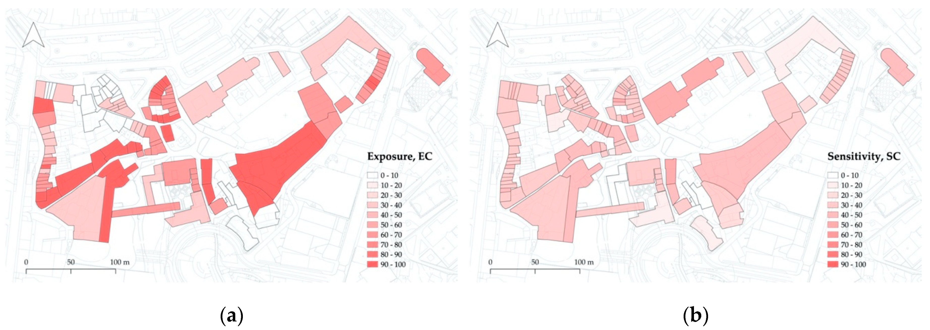
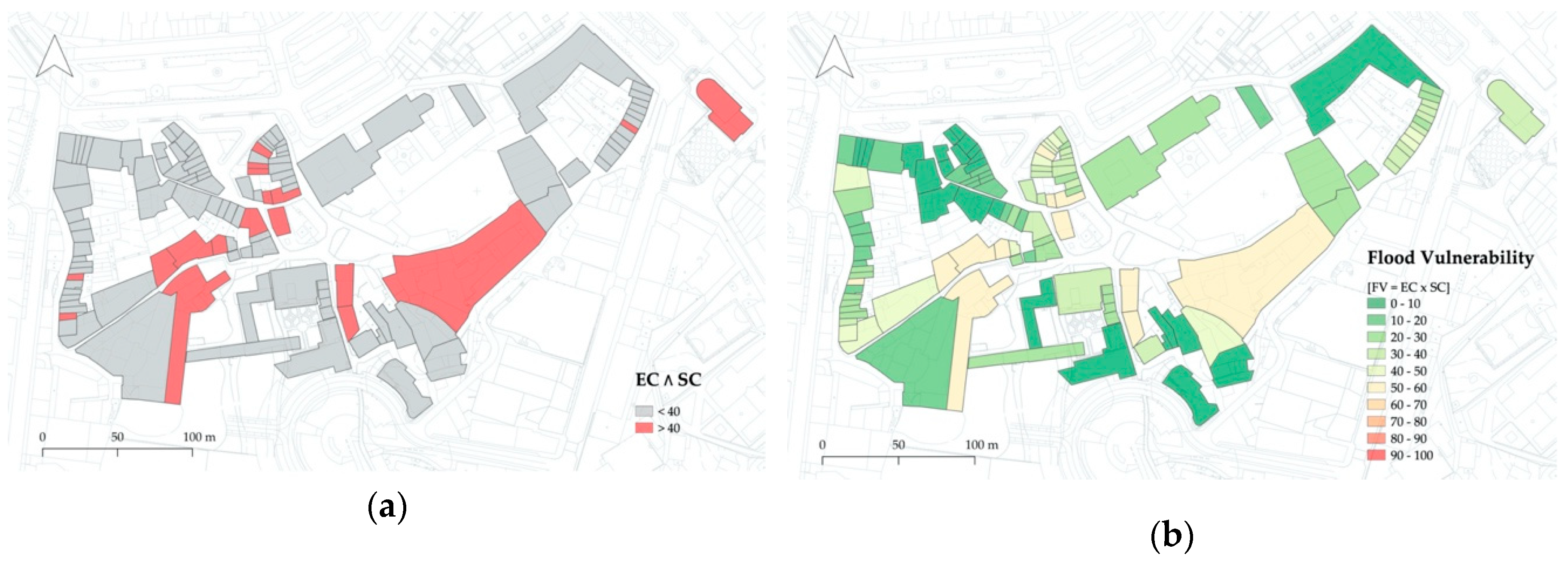
When getting into the discrete exposure, sensitivity, and vulnerability results, it is possible to gain a much better understanding of the overall vulnerability of the buildings. As illustrated in Figure 8a,b, respectively, spatial analysis reveals a scattered distribution of exposure and the sensitivity indicators over the study area. Comparatively, it is also clear that the exposure values are generally higher than sensitivity values. Despite this, and although there is no correlation between these two indicators, it is interesting to see that some of the most exposed buildings are also those that revealed to be more sensitive. This cross analysis is presented in Figure 9a, where we identify the buildings to which the exposure and the sensitivity values are cumulatively higher than 40. For vulnerability reduction purposes, these buildings are the most critical ones.
Figure 9b presents the distribution of the vulnerability index results. Although we have already commented on the most significant aspects when addressing the exposure and the sensitivity results, it is worth emphasising two further points. First, the fact that a significant part of the most vulnerable buildings is located in the central part of the study area. As we will have the opportunity to prove afterwards, this aspect may be essential, taking into account that these more vulnerable buildings are located coincidentally within the most hazardous area. Second, the fact that some of these buildings are abandoned. Keeping the social aspects out of the discussion, buildings’ abandonment is one of the main factors of rapid degradation and, as a result, increased physical vulnerability. During the discussion of the risk results, we will provide further insight into these critical issues.
4.3. Integrated Risk Assessment
After having discussed the main outputs resulting from the hazard and the vulnerability analysis, we are in an excellent position to integrate these results in order to obtain more comprehensive flood risk indicators. As detailed in Section 3.3, this integration will ultimately result in a risk matrix that correlates the level of vulnerability with the level of hazard to which each building is exposed. However, before going into such an outcome, we would like to analyse a set of second-order results obtained by crossing some of the above-discussed indicators.
4.3.1. Second-Order Analysis
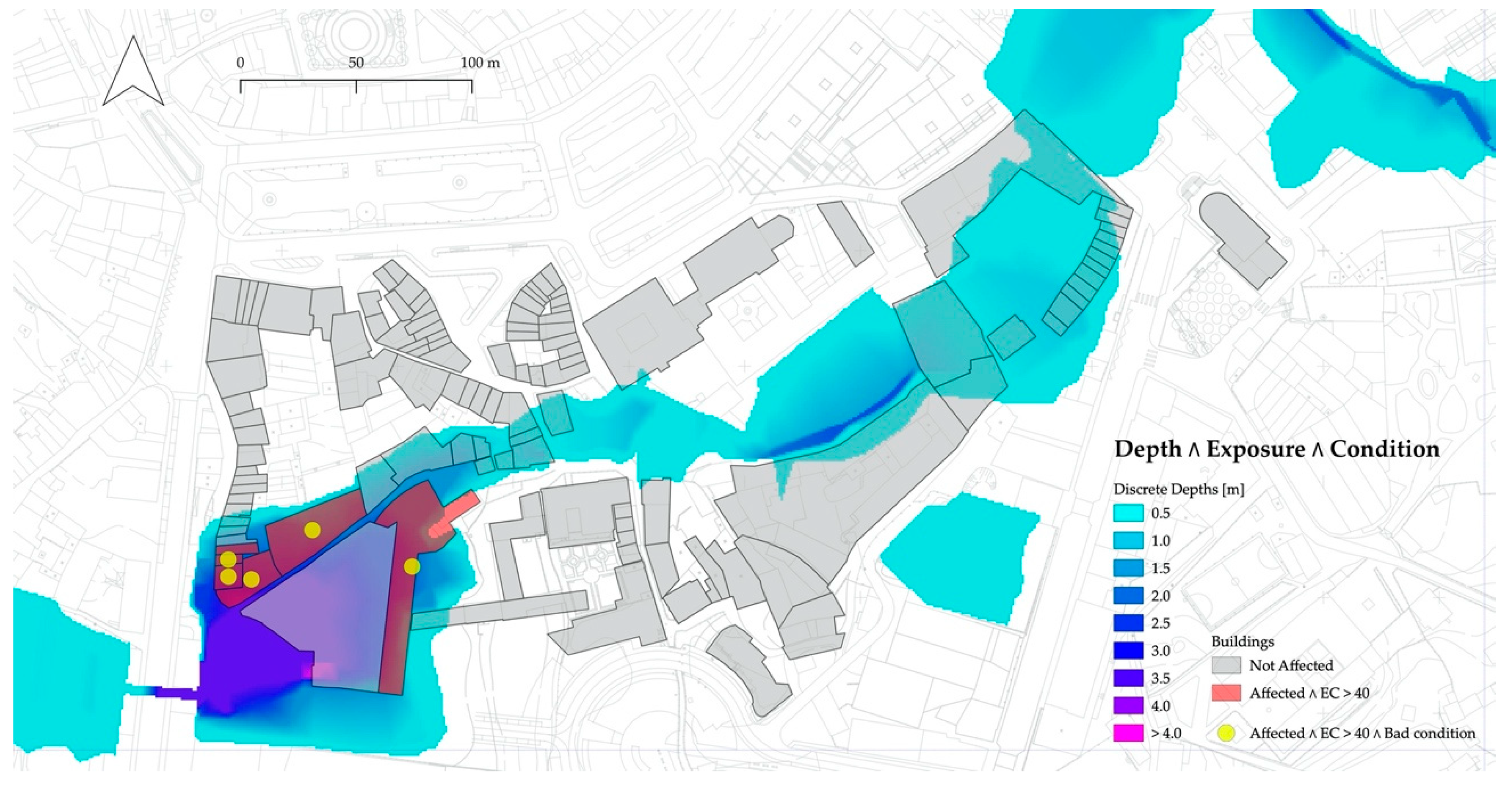
The first second-order result that we think is of great interest is the joint analysis of the water depth, the exposure component of the vulnerability index, and the conservation state of the buildings. Before going into the result, it is worth justifying the selection of these particular indicators. Water depth is recognised as the most relevant hazard indicator when analysing the impact of flood actions on buildings [15]: depth is usually used to produce vulnerability curves associated with flood events, which is also known as depth-damage curves [20,21,22]. In fact, although some studies note the importance of flood parameters other than depth [16], those are barely analysed so comprehensively. Equally important is the fact that water depth is directly related to flow velocity and, therefore, with the effects of the hydrodynamic actions. The impact of these hydrodynamic actions on the buildings are, of course, very dependent on their level of exposure—a building of which its façade wall is perpendicular to the direction of the water flow is potentially much more affected than another where its façade is parallel to the direction of the flow. As referred to in Section 3, this is exactly what the sensitivity component of the flood vulnerability index seeks to evaluate and that is why it is considered in this second-order analysis. It is also known that the weaker the state of conservation of the building, the higher the impact of the flood (due to hydrostatic and hydrodynamic actions). This fact rationalises the inclusion of this aspect in the present analysis.
Justifying the three indicators considered herein, Figure 10 presents the map resulting from their integrated analysis. We want to highlight a couple of interesting conclusions from the analysis of this map. The first one is the identification of highly-exposed buildings (i.e., with an EC value higher than 40) that, for the adopted 100-year peak flow scenario, are subject to a water depth over 2 m. Based on this first criterion, it is possible to identify six buildings—about 5% of the building stock within our study area—which are highlighted in red in Figure 10. However, when including the conservation state into the analysis, this number can be further reduced to 5 (about 4% of the building stock), making this result even more informative for decision-making purposes.
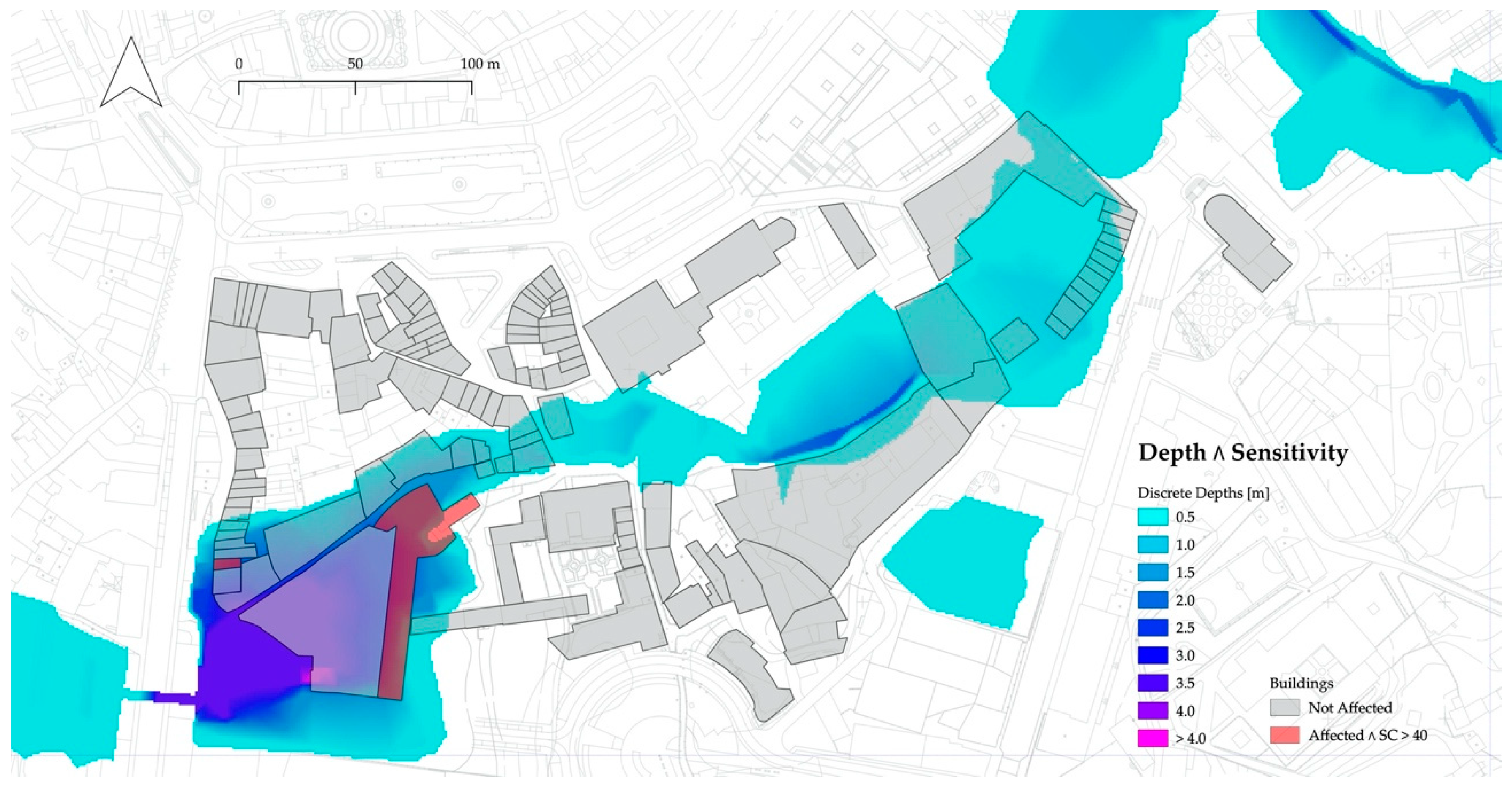
Another second-order result that we find worthy of particular discussion herein is the joint analysis of the water depth and the sensitivity component of the flood vulnerability index methodology. Since this component assesses the intrinsic characteristics of the buildings that make them sensitive to the impact of flood actions, it is undoubtedly relevant to consider these two indicators together. We would like to note that the conservation sate of the buildings is already part of the sensitivity component, which is why we now choose not to consider this aspect explicitly. Figure 11 presents the maps resulting from this analysis.
As can be inferred from the analysis of Figure 11, the number of buildings identified from the joint analysis of the water depth and the buildings’ sensitivity (for the very same 100-year peak flow scenario) is reduced to 2, which is a little less than 2%. It is also interesting to note that these two buildings are among the five already identified in Figure 10, which, from a decision-making standpoint, pushes them to the top of the intervention priorities.
4.3.2. Matrix-Based Analysis
After the above preliminary second-order analysis—through which we have already gained a deeper understanding about the potential impact of the considered flood scenario in some particular buildings—we got to the point of combining the obtained hazard and vulnerability results into a single flood risk indicator. As a result, the level of hazard and vulnerability associated with each building are related through a risk matrix, wherein the vulnerability is inputted directly using the flood vulnerability index (FV) and the hazard is derived from the velocity and water depth results, using Equation (2).
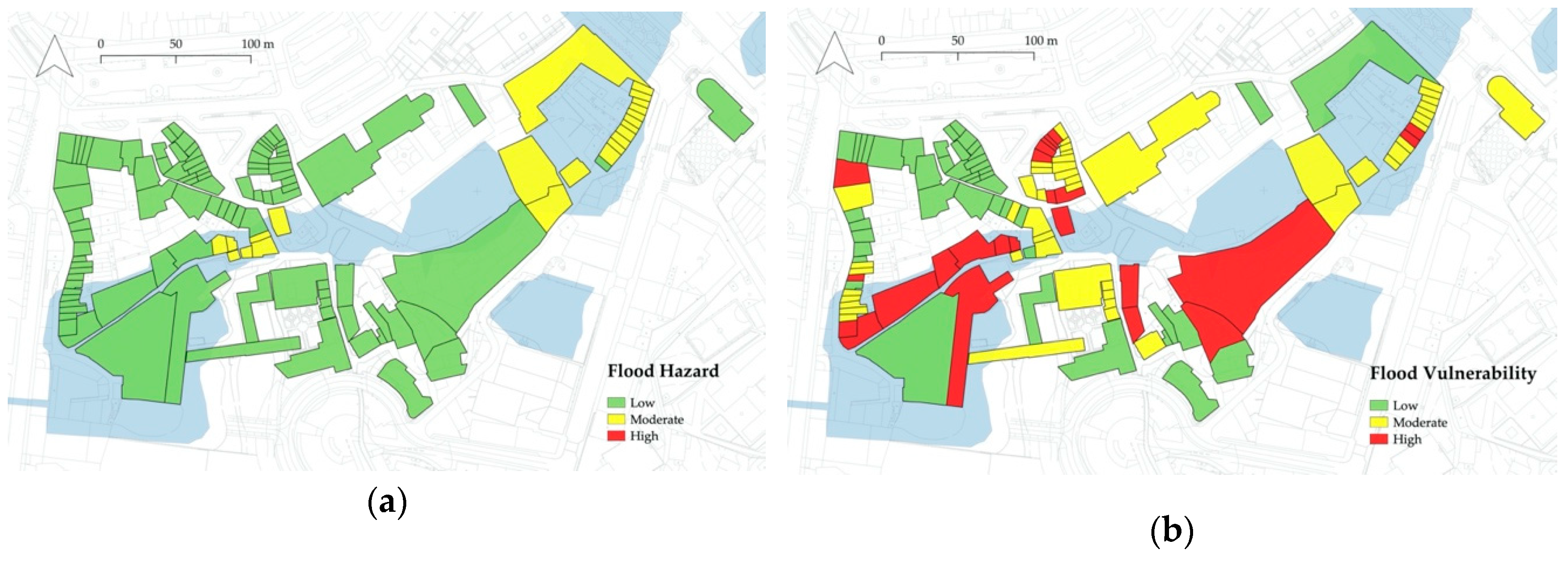
Thus, before diving deeper into the results obtained from the flood risk matrix, it is useful to map and analyse the spatial distribution of the hazard and vulnerability results. These maps are presented in Figure 12a,b. According to the criterion adopted in this matrix-based analysis, the level of flood hazard throughout the study area is quite homogeneous, see Figure 12a. Further, 22 out of the 116 buildings assessed (about 19%) were identified as having a “Moderate” flood hazard, whereas all the remaining were labelled with “Low” hazard. In terms of spatial distribution, it is possible to identify two blocks that can be particularly affected. Let us notice that although the hazard is being evaluated differently in this section—here, velocity and water depth are combined into a single hazard indicator—this result is in essential agreement with the discussion provided in Section 4.1. As for the spatial distribution of the flood vulnerability results, given in Figure 12b, it is visibly more heterogeneous: 37.9% (44), 41.4% (48), and 20.7% (24) of the buildings were identified as having a “Low”, “Moderate”, and “High” flood vulnerability, respectively.
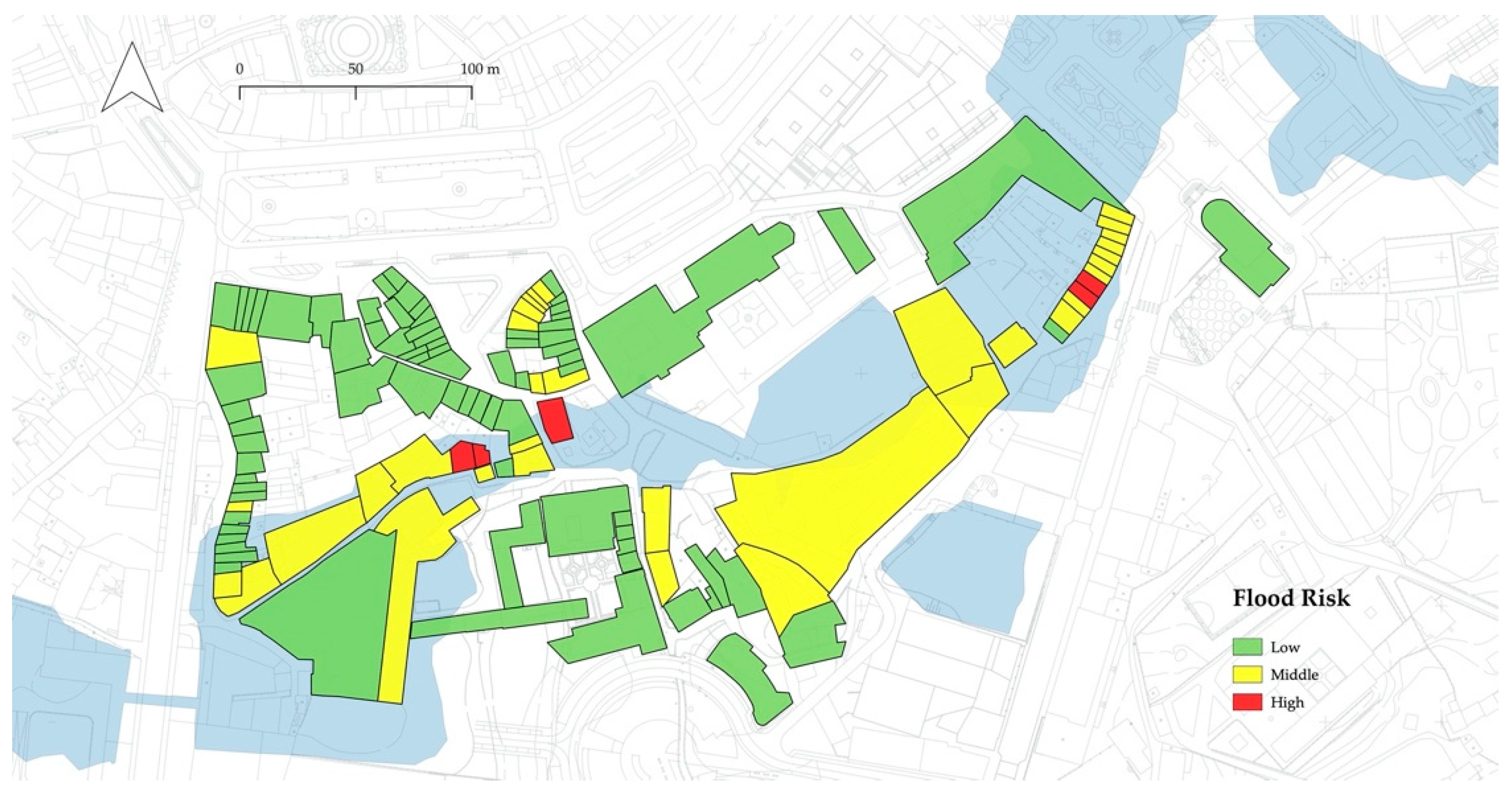
Contextualising the hazard and the vulnerability results, it remains for us to present and discuss the final flood risk results. They are illustrated in Figure 13 and quantified in Table 3.
As shown in the flood risk matrix provided in Table 5, 66.4% of the buildings (77) were identified with “Low” flood risk, 29.3% (34) with “Middle” risk, and 4.3% (5) with “High” risk for the same 100-year peak flow scenario considered in this work.
Complementarily to the main conclusions drawn from the second-order analysis discussed in Section 4.3.1, this outcome allows us to recognise some additional buildings that, because the hydrodynamics effects of the flood have been disregarded in that analysis (only water depth was considered explicitly), are not identified there. In fact, none of the building previously highlighted in Figure 10 and Figure 11 are identified in this final analysis as having a “High” flood risk. If in a less thoughtful consideration these two results may seem divergent, in fact, they prove to us the importance of considering different criteria and approaches to assess flood risk in urban areas. Still, in this regard, we would like to stress that these results are obviously conditioned by the criterion used to define the levels of hazard and vulnerability. If, for example, we had used a different criterion from that given by Equation (2)—which, as is always the case, was proposed by Clausen [15] from a set of specific conditions—the results could be very different. This said, the five buildings identified in this analysis, together with those five identified in Section 4.3.1, should be the priority targets of future flood risk mitigation programs.
5. Conclusions
This paper presents a new method for assessing the flood risk of the built environment, specifically adapted to areas classified by their heritage value. For the effect, the Historic City Centre of Guimarães (Portugal) was selected as a study area.
We have defined a hazard scenario for the 100-year flood by hydraulic modelling with HEC-RAS, of which its outputs are flood extent, depth, and velocity. Such outputs, derived from a steady flow analysis, must assume the limitation of not providing information that ultimately would allow for a better understanding of the flooding process, namely that from a flood hydrograph (time to peak and duration of inundation), an unsteady analysis would result. The vulnerability has been assessed by considering an exposure component (based on wall orientation) and a sensitivity component (based on heritage status, age, number of storeys, condition, and material of buildings). They define the hazard and vulnerability modules of a GIS tool, which later provided a cross-analysis of information, culminating in a flood risk matrix. A total of 116 buildings were evaluated with the developed methodology.
The first insight into each module’s results provided a detailed understanding of flood risk roots or causes, which gives decision-makers and planners information on which risk factors are more relevant in each block or building. This highlighted wall orientation and condition as the most concerning aspects, with exposure being more relevant than sensitivity in explaining physical vulnerability. The second-order analysis evaluated evidence risk contexts that otherwise would go unnoticed, namely a) the analysis of flood depths, conservation state (from the sensitivity component of FV), and wall orientation (from the exposure component of FV) and b) the overlay of flood depths with the sensitivity component of FV. Complementarily, the risk-matrix analysis identified other buildings as high risk, some of them not coincident with the individualised analysis of risk components (hazard and vulnerability).
It is the ability to characterise the potential impacts of hazardous processes that allows us to prepare and promote the necessary formal and informal changes, which, ultimately, will contribute to risk reduction [23]. In that sense, we expect the generated knowledge to be applicable in different fields of flood risk management.
If the individual first-order results are used, resources’ assignment will prove to be more efficient in addressing the particular risk factors identified as more relevant in each building. Combined with the risk-matrix classification, the results are capable of informing municipal decision-makers and planners regarding the intervention priorities of urban rehabilitation projects. Civil protection agents will be capable of planning efficient and safe evacuation routes, in case of flash flooding. The business sector will be able to prepare for recurrent flooding with minor consequences, defined by some as nuisance flooding. Finally, medium- to long-term strategies of spatial planning and design can be drawn from the risk-matrix results: the eventual relocation of buildings classified as high risk; the retrofitting of their physical characteristics in order to reduce their physical vulnerability while maintaining their functionality, if possible, even during flood events, in the areas of low risk. Intermediate contexts of flood risk require, in terms of spatial and design planning, pondering the range of possible interventions, specifically those that better combine urbanity and safety in distinct degrees of flood adaptation [24].
When coupled with social vulnerability data, the provided risk assessment will significantly contribute to increasing the resilience of the built environment. The historical centres of cities represent places of high sensitivity of their exposed elements. In addition to their heritage and cultural value, the mandated authorities need to consider the functions that these buildings provide, both for the resident population and the transient population.
The analysis we have presented, although focused on flood risk, can be replicated with some adaptation, concerning other hazard processes, not exclusively of hydro-geomorphologic origin. Moreover, provided that the evaluated buildings can be grouped typologically, we believe that this framework can be easily applied in larger-scale risk assessments, keeping a very reasonable balance between accuracy and applicability. In that case, blocks of buildings or even entire neighbourhoods can be used as the basic assessment units. An interesting example of using neighbourhoods as the basic assessment unit to evaluate fire risk can be found in [25].
Author Contributions
Conceptualisation, T.M.F. and P.P.S.; methodology, T.M.F. and P.P.S.; hazard analysis, P.P.S.; vulnerability analysis, T.M.F.; investigation, T.M.F. and P.P.S.; writing—original draft preparation, T.M.F. and P.P.S.; writing—review and editing, T.M.F. and P.P.S.; funding acquisition, T.M.F. and P.P.S. All authors have read and agreed to the published version of the manuscript.
Funding
Tiago M. Ferreira is funded by the Portuguese Foundation for Science and Technology (FCT) through the postdoctoral grant SFRH/BPD/122598/2016 and Pedro P. Santos is funded through the project with the reference CEEIND/00268/2017.
Acknowledgments
The authors would like to acknowledge the City Council of Guimarães, particularly the Architect Filipe Fontes, for his generous support and contribution to the development of this work.
Conflicts of Interest
The authors declare no conflict of interest.
References
- UNISDR. 2009 UNISDR Terminology on Disaster Risk Reduction; International Strategy for Disaster Reduction: Geneva, Switzerland, 2009; ISBN 978-600-6937-11-3. [Google Scholar]
- Rana, I.A.; Routray, J.K. Integrated methodology for flood risk assessment and application in urban communities of Pakistan. Nat. Hazards 2018, 91, 239–266. [Google Scholar] [CrossRef]
- Birkmann, J.; Cardona, O.D.; Carreño, M.L.; Barbat, A.H.; Pelling, M.; Schneiderbauer, S.; Kienberger, S.; Keiler, M.; Alexander, D.; Zeil, P.; et al. Framing vulnerability, risk and societal responses: The MOVE framework. Nat. Hazards 2013, 67, 193–211. [Google Scholar] [CrossRef]
- Ortiz, R.; Ortiz, P.; Martín, J.M.; Vázquez, M.A. A new approach to the assessment of flooding and dampness hazards in cultural heritage, applied to the historic centre of Seville (Spain). Sci. Total Environ. 2016, 551–552, 546–555. [Google Scholar] [CrossRef] [PubMed]
- Wang, J.-J. Flood risk maps to cultural heritage: Measures and process. J. Cult. Herit. 2015, 16, 210–220. [Google Scholar] [CrossRef]
- Miranda, F.N.; Ferreira, T.M. A simplified approach for flood vulnerability assessment of historic sites. Nat. Hazards 2019, 96, 713–730. [Google Scholar] [CrossRef]
- Marzeion, B.; Levermann, A. Loss of cultural world heritage and currently inhabited places to sea-level rise. Environ. Res. Lett. 2014, 9, 34001. [Google Scholar] [CrossRef]
- Granda, S.; Ferreira, T.M. Assessing Vulnerability and Fire Risk in Old Urban Areas: Application to the Historical Centre of Guimarães. Fire Technol. 2019, 55, 105–127. [Google Scholar] [CrossRef]
- Ramísio, P.; Duarte, A.; Vieira, J. Integrated flood management in urban environment: A case study. In Proceedings of the XIV World Water Congress “Bridging Science and Policy”, Porto-da-Galinhas, Brazil, 25–29 September 2011. [Google Scholar]
- Zêzere, J.L.; Pereira, S.; Tavares, A.O.; Bateira, C.; Trigo, R.M.; Quaresma, I.; Santos, P.P.; Santos, M.; Verde, J. DISASTER: A GIS database on hydro-geomorphologic disasters in Portugal. Nat. Hazards 2014, 72, 503–532. [Google Scholar] [CrossRef]
- Ramísio, P.; Duarte, A.; Vieira, J. Estudo Hidrológico e Modelação Hidrodinâmica: Estudo hidrológico da bacia hidrográfica da ribeira de Couros; University of Minho: Guimarães, Portuga, 2011. [Google Scholar]
- Ramísio, P.; Duarte, A.; Vieira, J. Estudo Hidrológico e Modelação Hidrodinâmica: Modelação hidrodinâmica da ribeira de Couros—Situação de referência; University of Minho: Guimarães, Portugal, 2012. [Google Scholar]
- USACE HEC-RAS. River Analysis System. In Hydraulic Reference Manual; US Army Corps of Engineers, Hydrologic Engineering Center: Davis, CA, USA, 2016; p. 547. Available online: https://www.hec.usace.army.mil/software/hec-ras/documentation/HEC-RAS%205.0%20Reference%20Manual.pdf (accessed on 8 June 2020).
- Vicente, R.; Parodi, S.; Lagomarsino, S.; Varum, H.; Silva, J.A.R.M. Seismic vulnerability and risk assessment: Case study of the historic city centre of Coimbra, Portugal. Bull. Earthq. Eng. 2011, 9, 1067–1096. [Google Scholar] [CrossRef]
- Clausen, L. Potential Dam Failure: Estimation of Consequences, and Implications for Planning. Unpublished Master’s Thesis, School of Geography and Planning at Middlesex Polytechnic Collaborating with Binnie and Partners, Redhill, UK, 1989. [Google Scholar]
- Kelman, I.; Spence, R. An overview of flood actions on buildings. Eng. Geol. 2004, 73, 297–309. [Google Scholar] [CrossRef]
- QGIS Development Team. QGIS Geographic Information System; Open Source Geospatial Foundation: Beaverton, OR, USA, 2017. [Google Scholar]
- Stephenson, V.; D’Ayala, D. A new approach to flood vulnerability assessment for historic buildings in England. Nat. Hazards Earth Syst. Sci. 2014, 14, 1035–1048. [Google Scholar] [CrossRef] [Green Version]
- Mebarki, A.; Valencia, N.; Salagnac, J.L.; Barroca, B. Flood hazards and masonry constructions: A probabilistic framework for damage, risk and resilience at urban scale. Nat. Hazards Earth Syst. Sci. 2012, 12, 1799–1809. [Google Scholar] [CrossRef]
- McBean, E.A.; Gorrie, J.; Fortin, M.; Ding, J.; Moulton, R. Flood Depth—Damage Curves By Interview Survey. J. Water Resour. Plan. Manag. 1988, 114, 613–634. [Google Scholar] [CrossRef]
- Pistrika, A.; Tsakiris, G.; Nalbantis, I. Flood Depth-Damage Functions for Built Environment. Environ. Process. 2014, 1, 553–572. [Google Scholar] [CrossRef] [Green Version]
- Velasco, M.; Cabello, À.; Russo, B. Flood damage assessment in urban areas. Application to the Raval district of Barcelona using synthetic depth damage curves. Urban Water J. 2016, 13, 426–440. [Google Scholar] [CrossRef]
- Birkmann, J.; Buckle, P.; Jaeger, J.; Pelling, M.; Setiadi, N.; Garschagen, M.; Fernando, N.; Kropp, J. Extreme events and disasters: A window of opportunity for change? Analysis of organisational, institutional and political changes, formal and informal responses after mega-disasters. Nat. Hazards 2010, 55, 637–655. [Google Scholar] [CrossRef]
- Hobeica, L.; Santos, P. Design with floods: From defence against a ‘Natural’ threat to adaptation to a human-natural process. Int. J. Saf. Secur. Eng. 2016, 6, 616–626. [Google Scholar] [CrossRef] [Green Version]
- Granda, S.; Ferreira, T.M. Large-scale Vulnerability and Fire Risk Assessment of the Historic Centre of Quito, Ecuador. Int. J. Archit. Herit. 2019, 1–15. [Google Scholar] [CrossRef]
Figure 1.
The Historic City Centre of Guimarães: (a) View to one of its squares; (b) Example of a flood event in the Couros’ river basin (source: Guimarães City Council).
Figure 1.
The Historic City Centre of Guimarães: (a) View to one of its squares; (b) Example of a flood event in the Couros’ river basin (source: Guimarães City Council).

Figure 2.
The conceptual framework of the integrated flood risk assessment approach.

Figure 3.
The schematisation of the vulnerability module.

Figure 4.
Flood inundation map for the adopted 100-year peak flow scenario.

Figure 5.
Flood velocities resulted from the adopted 100-year peak flow scenario.

Figure 6.
Water depth resulted from the adopted 100-year peak flow scenario.

Figure 7.
Mapping of the spatial distribution of the vulnerability classes: (a) Wall Orientation; (b) Building Material; (c) Condition (or conservation status); (d) Number of Storeys; (e) Building Age; (f) Heritage Status.
Figure 7.
Mapping of the spatial distribution of the vulnerability classes: (a) Wall Orientation; (b) Building Material; (c) Condition (or conservation status); (d) Number of Storeys; (e) Building Age; (f) Heritage Status.

Figure 8.
Spatial distribution of the exposure (a) and the sensitivity (b) indicators.

Figure 9.
Cross analysis of the exposure and the sensitivity indicators (a) and spatial distribution of the vulnerability index results (b).
Figure 9.
Cross analysis of the exposure and the sensitivity indicators (a) and spatial distribution of the vulnerability index results (b).

Figure 10.
Joint analysis of water depth, exposure, and condition indicators.

Figure 11.
Joint analysis of water depth and the sensitivity indicator.

Figure 12.
Spatial distribution of the flood hazard (a) and flood vulnerability results (b).

Figure 13.
Spatial distribution of the flood risk results.


Table 1.
Estimated flow data for use in the hydraulic model of the Couros river reach, in the Historic City Centre of Guimarães.
Table 1.
Estimated flow data for use in the hydraulic model of the Couros river reach, in the Historic City Centre of Guimarães.
| Pour Point | Upstream Inlet | A | B | C | D | E | F | G | H | I | J | K |
|---|---|---|---|---|---|---|---|---|---|---|---|---|
| Reach length (m) | 0.00 | 33.0 | 51.6 | 158.9 | 260.0 | 651.2 | 782.7 | 1013.7 | 1146.4 | 1252.6 | 1344.2 | 1495.1 |
| Affluent Qp (m3/s) | 35.95 | 0.45 | 1.53 | 0.60 | 2.00 | 1.16 | 0.32 | 1.97 | 7.55 | 0.38 | 0.97 | 1.27 |
| Sum Qp (m3/s) | 35.95 | 36.40 | 37.93 | 38.53 | 40.53 | 41.69 | 42.01 | 43.98 | 51.53 | 51.91 | 52.88 | 54.15 |
Table 2.
Flood risk matrix.
| Flood Risk | Hazard | |||
| Low | Moderate | High | ||
| Vulnerability | High | Middle Risk | High Risk | High Risk |
| Moderate | Low Risk | Middle Risk | High Risk | |
| Low | Low Risk | Low Risk | Middle Risk | |
Table 3.
Number of affected building distributed by ranges of the affected extent.
| Flood Extent | Range of Values | |||||
| >0–20 | 20–40 | 40–60 | 60–80 | 80–<100 | Fully affected | |
| Affected Buildings | 4 (9.76%) | 2 (4.88%) | 4 (9.76%) | 1 (2.44%) | 7 (17.07%) | 23 (56.10%) |
Table 4.
Number of affected buildings distributed by ranges of flood velocity and water depth.
| Hazard Indicator | Range of Values | ||||||||
| 0–0.5 | 0.5–1.0 | 1.0–1.5 | 1.5–2.0 | 2.0–2.5 | 2.5–3.0 | 3.0–3.5 | 3.5–4.0 | >4.0 | |
| Velocity (m/s) | 12 (29.3%) | 3 (7.3%) | 1 (2.4%) | 3 (7.3%) | 5 (12.2%) | 5 (12.2%) | 4 (9.8%) | 3 (7.3%) | 5 (12.2%) |
| Depth (m) | 10 (24.4%) | 15 (36.6%) | 4 (9.8%) | 5 (12.2%) | 2 (4.9%) | 2 (4.9%) | 1 (2.4%) | 1 (2.4%) | 1 (2.4%) |
Table 5.
Flood risk matrix.
| Flood Risk | Hazard | |||
| Low | Moderate | High | ||
| Vulnerability | High | 19 (16.4%) Middle Risk | 5 (4.3%) High Risk | 0 High Risk |
| Moderate | 33 (28.5%) Low Risk | 15 (12.9%) Middle Risk | 0 High Risk | |
| Low | 42 (36.2%) Low Risk | 2 (1.7%) Low Risk | 0 Middle Risk | |
© 2020 by the authors. Licensee MDPI, Basel, Switzerland. This article is an open access article distributed under the terms and conditions of the Creative Commons Attribution (CC BY) license (http://creativecommons.org/licenses/by/4.0/).
Share and Cite
MDPI and ACS Style
Ferreira, T.M.; Santos, P.P. An Integrated Approach for Assessing Flood Risk in Historic City Centres. Water 2020, 12, 1648. https://0-doi-org.brum.beds.ac.uk/10.3390/w12061648
AMA Style
Ferreira TM, Santos PP. An Integrated Approach for Assessing Flood Risk in Historic City Centres. Water. 2020; 12(6):1648. https://0-doi-org.brum.beds.ac.uk/10.3390/w12061648
Chicago/Turabian StyleFerreira, Tiago M., and Pedro P. Santos. 2020. "An Integrated Approach for Assessing Flood Risk in Historic City Centres" Water 12, no. 6: 1648. https://0-doi-org.brum.beds.ac.uk/10.3390/w12061648
Note that from the first issue of 2016, this journal uses article numbers instead of page numbers. See further details here.