Quantile Analysis of Long-Term Trends of Near-Surface Chlorophyll-a in the Pearl River Plume

Abstract

The concentration of chlorophyll-a (CHL) is an important proxy for the amount of phytoplankton biomass in the ocean. Characterizing the variability of CHL in the Pearl River Plume (PRP) is therefore of great importance for the understanding of the changes in oceanic productivity in the coastal region. By applying quantile regression analysis on 21-year (1998–2018) near-surface CHL data from satellite observations, this study investigated the long-term trend of CHL in the PRP. The results show decreasing trends (at an order of 10⁻² mg m⁻³ year⁻¹) for all percentiles of the CHL in the PRP, suggesting a decrease in productivity in the past two decades. The trends differ fundamentally from those in the open regions of the northern South China Sea with mixed signs and small magnitudes (10⁻⁴ mg m⁻³ year⁻¹). The magnitudes of the trends in high quantiles (>80th) are larger than those in low quantiles (<50th) in the PRP, indicative of a decrease in the variance of the CHL. The area with apparent decreasing trends is restricted to the PRP in summer and extends to the entire coastal region in winter. This decrease in CHL is possibly attributed to the decrease in nutrient input from the river runoff and the weakening of wind-forced mixing rather than the changes in sea surface temperature. This study extends our knowledge on the variability of CHL in the PRP and provides references to the investigation of the changes of the coastal ecological environment.

1. Introduction

The Pearl River (PR) is the second largest river in terms of water discharge in China [1]. The Pearl River Plume (PRP) is formed by the PR discharge, which expands hundreds of kilometers away from the estuary into the northern South China Sea (NSCS) (Figure 1). This river plume forms a critical area of intense physical and biogeochemical land–ocean interactions. The PR delivers terrestrial freshwater into the NSCS at an average annual discharge rate of 300 km³ year⁻¹ [1,2]. About 80% of the river runoff occurs during the wet season (from April to September) [2,3]. The discharged freshwater with a huge amount of terrestrial nutrient spreads over abroad the continental shelf and stimulates algal blooms, playing essential roles in modulating the biogeochemical environments in the PRP [4].

River plume generally yields a right-tilted bulge of terrestrial freshwater at the estuary due to the β effect (in the northern hemisphere) [5]. However, the northern coast of the SCS experiences seasonally inverse monsoon, which modifies the coastal currents and thus the extending of the PRP [6,7]. During winter, the prevailing northeast monsoon produces shoreward Ekman transport, which impedes the offshore dispersal of the plume and drives the plume spreading westward along with the current [8]. In summer, the southwest monsoon gives rise to offshore Ekman transport and coastal upwelling, which promote the offshore and eastward extending of the river plume [9,10]. The input of nutrients from the PR facilitates the growth of phytoplankton and enhances productivity in the coastal ocean [5,11,12]. As demonstrated by Gan et al. [13], wind-driven coastal currents can transport nutrient-rich water stretching eastward from the PR estuary over the middle shelf and form a long tongue-shaped phytoplankton bloom in summer. Other dynamical processes, such as tides, mesoscale eddies, and tropical cyclones, have also been reported to promote the expansion of the plume and initiate phytoplankton blooms [14,15,16].

The concentration of chlorophyll-a (CHL) has been widely used as a proxy for the amount of phytoplankton biomass in the ocean [17,18,19]. Characterizing the variability of CHL in the PRP is therefore of great importance for the understanding of the changes in oceanic productivity in the coastal region. Numerous studies have revealed that the concentrations of CHL in the NSCS are high in winter due to deep convective mixing and low in summer because of intense upper ocean stratification [19,20,21,22]. However, the input of nutrients from the PR adds complexity to the variability of biogeochemical environments in the northern coast of the NSCS. Few studies have focused on the temporal variation of CHL in the coastal regions yet. It is not clear whether the river discharge influences the seasonal cycles and the long-term variability of the CHL.

Quantifying the long-term variability of CHL is a challenging task. Previous studies often focused on regression analyses that compute the climate trend of the mean values of CHL based on the least-squares method [19,23,24]. However, this method only provides information about the trend of mean values. Variability in other parts of the CHL distribution can sometimes be equally or more important than the changes in mean values [25]. For example, changes in high CHL values that represent phytoplankton blooms can considerably impact coastal fisheries and aquaculture. Recently, quantile regression has been developed as an extension to the ordinary regression analysis [26]. The specificity of this method is that it estimates a range of trends of conditional quantiles of the dependent variable instead of the conditional mean [25]. The method provides a more complete description of the long-term variability of a time series and is especially useful in applications where extremes are important [27]. The quantile regression analysis has been widely used in the studies of the long-term trends of land temperature [27,28,29,30], precipitation [31], sea ice [32], and sea level [25].

In this work, we apply the quantile regression analysis on 21-year (1998–2018) near-surface CHL data from satellite observations to derive a comprehensive description of the long-term variability of CHL in the PRP. Simultaneous variations of PR discharge, sea surface wind, and sea surface temperature (SST) are also analyzed to reveal the possible factors responsible for the long-term changes in the CHL.

2. Data and Methods

2.1. Data

The merged CHL data with a temporal resolution of 8 days and a spatial resolution of 4 km between 1998 and 2019 were derived from the GlobColour Project. The data were constructed by merging observations from multiple satellites (i.e., Sea-viewing Wide Field-of-view Sensor (SeaWiFS), Moderate Resolution Imaging Spectroradiometer (MODIS), Medium Resolution Imaging Spectrometer (MERIS) and Visible Infrared Imaging Radiometer Suite (VIIRS)) using the Garver-Siegel-Maritorena (GSM) semianalytical ocean color algorithm [33]. These merged data were used because satellite ocean color observations are often soiled by clouds and result in data gaps. The merging of data from multiple satellites that have various transit times significantly increases (by 23%–80%) the spatial coverage of the data from any single mission [33]. Although the uncertainty of remotely-sensed CHL rises in coastal regions due to increased turbidity, studies have confirmed that the observations can capture the general spatial and temporal variations of the CHL distributions [13,34,35,36].

The sea surface wind data used in this study were the version 7.0.1 products of WindSat data produced by Remote Sensing Systems (RSS). The data have a spatial resolution of 25 km and a temporal resolution of 7 days. The data are available between February 2003 and December 2019. Although the time length of this data is shorter than that of the CHL data, it is longer than those of the wind data form Quick Scatterometer (QuikSCAT, 1999–2009) and Advanced Scatterometer (ASCAT, 2007–2019). The SST data used in this study were the level-4 products of the Group for High Resolution Sea Surface Temperature (GHRSST). The dataset was generated by combining complementary satellite and in situ observations within Optimal Interpolation systems. These data were chosen because they are gap-free, which means they have a much higher spatial coverage than the SST data from single satellites, such as MODIS. These data have a spatial resolution of 4 km and a temporal resolution of 1 day and are available between April 2006 and December 2019. The annual mean PR discharge and sediment data were derived from the Bulletins of Chinese River Sediment (1998–2018).

2.2. Methods

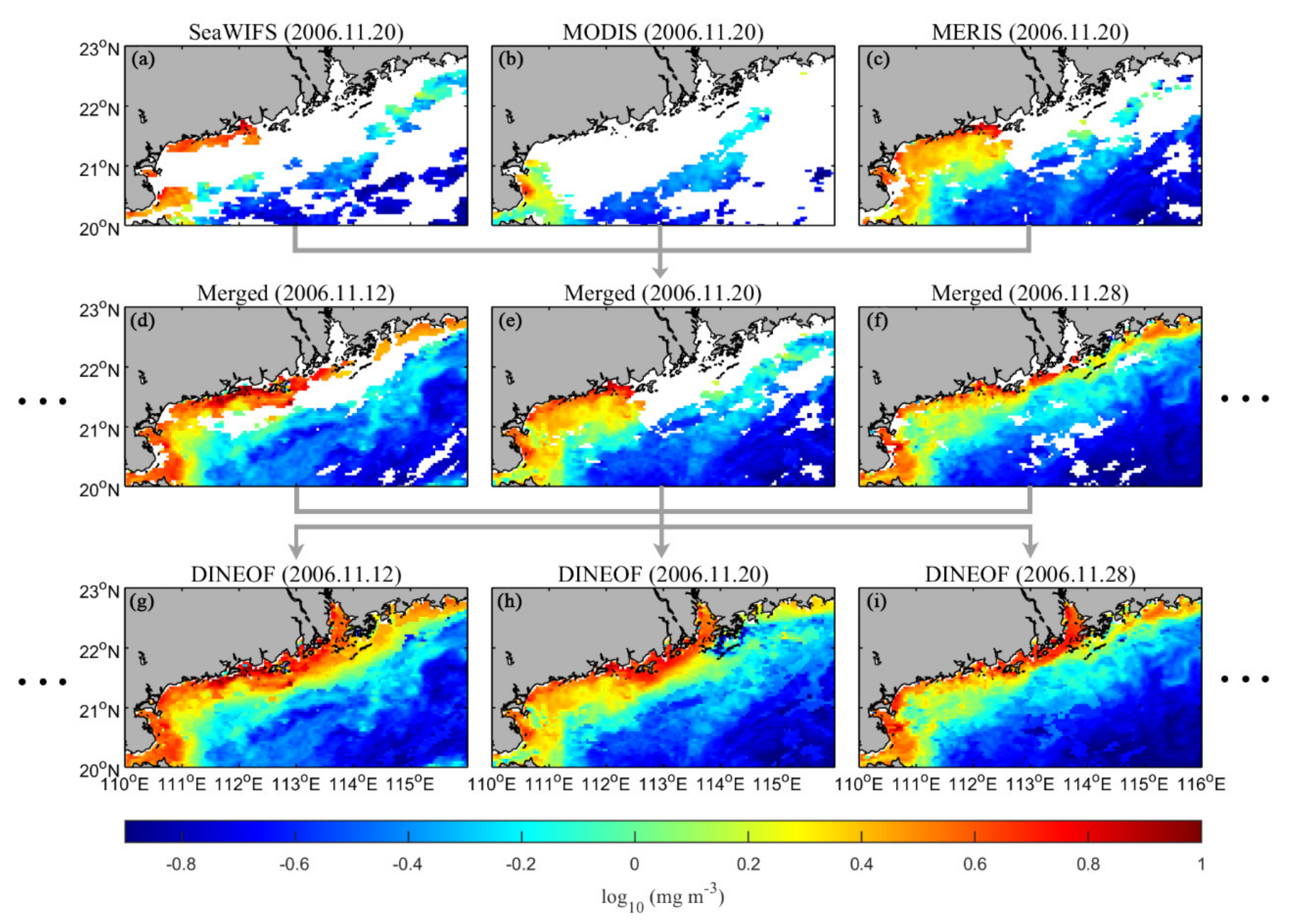
The quantile regression favors a complete time series of input data without missing values. Although the data coverage is improved, the merged CHL data still have data gaps (Figure 2, top two rows). We, therefore, applied the Data Interpolating Empirical Orthogonal Functions (DINEOF) to reconstruct the missing values before the quantile analysis (Figure 2, bottom row). The DINEOF is an EOF-based approach to reconstruct missing data in geophysical datasets [37]. It exploits an optimal number of EOFs determined by a cross-validation technique to infer values at missing locations. The method has a distinct advantage as a self-consistent, parameter-free technique without the need for a priori information [38]. This technique has been widely used to infer the missing values in ocean color data [39,40,41,42] and has been demonstrated able to reproduce the high spatial and temporal oceanic variability signals in the reconstructed data [43]. A detailed introduction to the DINEOF can be found in Beckers and Rixen [37] and Alvera-Azcárate et al. [38].

Quantile regression can be considered as an extension of ordinary regression based on the least square method [44]. For linear regression, the response variable (y) is linearly correlated with the independent variable (x): y = αx + β, where α is the linear slope and β the intercept. This is an estimate of conditional expectation function E(y|x). The parameters α and β are estimated by solving the problem of minimizing the sum of squared residuals:

$$\min {\displaystyle \sum }_{i=1}^n{\left(y_i-\left(\alpha {\mathrm{x}}_i+\beta \right)\right)}^2$$

(1)

Quantile regression can be easily understood if we replace the conditional mean function by a conditional quantile function [25]. That is replacing the mean of the response variable by the quantile of the response variable: y = ${\alpha }_{\tau }$x + ${\beta }_{\tau }$, where ${\alpha }_{\tau }$ is the quantile slope and ${\beta }_{\tau }$ the intercept for quantile τ [45]. Then, for each quantile ranging from 0 to 1, the two parameters are estimated by solving the problem of minimizing the sum of asymmetrically weighted absolute residuals instead of squared residuals:

$$\min {\sum }_{i=1}^n{\rho }_{\tau }\left(y_i-\left({\alpha }_{\tau }{\mathrm{x}}_i+{\beta }_{\tau }\right)\right),$$

(2)

where ${\rho }_{\tau }$ is the tilted absolute value function, which gives different weights to positive and negative residuals [25,44]:

$${\rho }_{\tau }=\left\{\begin{array}{cc}\tau ,& y_i\ge \left({\alpha }_{\tau }{\mathrm{x}}_i+{\beta }_{\tau }\right)\\ 1-\tau ,& y_i<\left({\alpha }_{\tau }{\mathrm{x}}_i+{\beta }_{\tau }\right)\end{array}\right.$$

(3)

3. Results

The northern coast of the NSCS is characterized by especially high concentrations of CHL in the PRP (Figure 1a). The annual mean concentration of CHL in the PR estuary is 3.3 mg m⁻³, which is approximately 50% higher than those in the western and eastern coastal regions. The concentrations of CHL decrease dramatically offshore to 1 mg m⁻³ at 50 m isobaths and to 0.3 mg m⁻³ at 100 m isobaths, resulting in markedly CHL fronts meandering along the shelf. These features present the importance of PR discharge in increasing productivity in the coastal regions.

The PR discharge not only results in high CHL in the river plume but also modifies the seasonality of the CHL. As presented in Figure 1c, the concentrations of CHL in the PRP are high in summer and low in winter, opposing to the seasonality of CHL in the open regions of the NSCS (Figure 1d). For most regions south of 21.3° N, the concentrations of CHL reach the maximum in December or January (winter) (Figure 1b). However, for the northern regions, the concentrations of CHL reach the maximum in June or July (summer). The feature indicates that the influence of the river discharge on regional biogeochemical environments can extend southward for 100 km from the estuary.

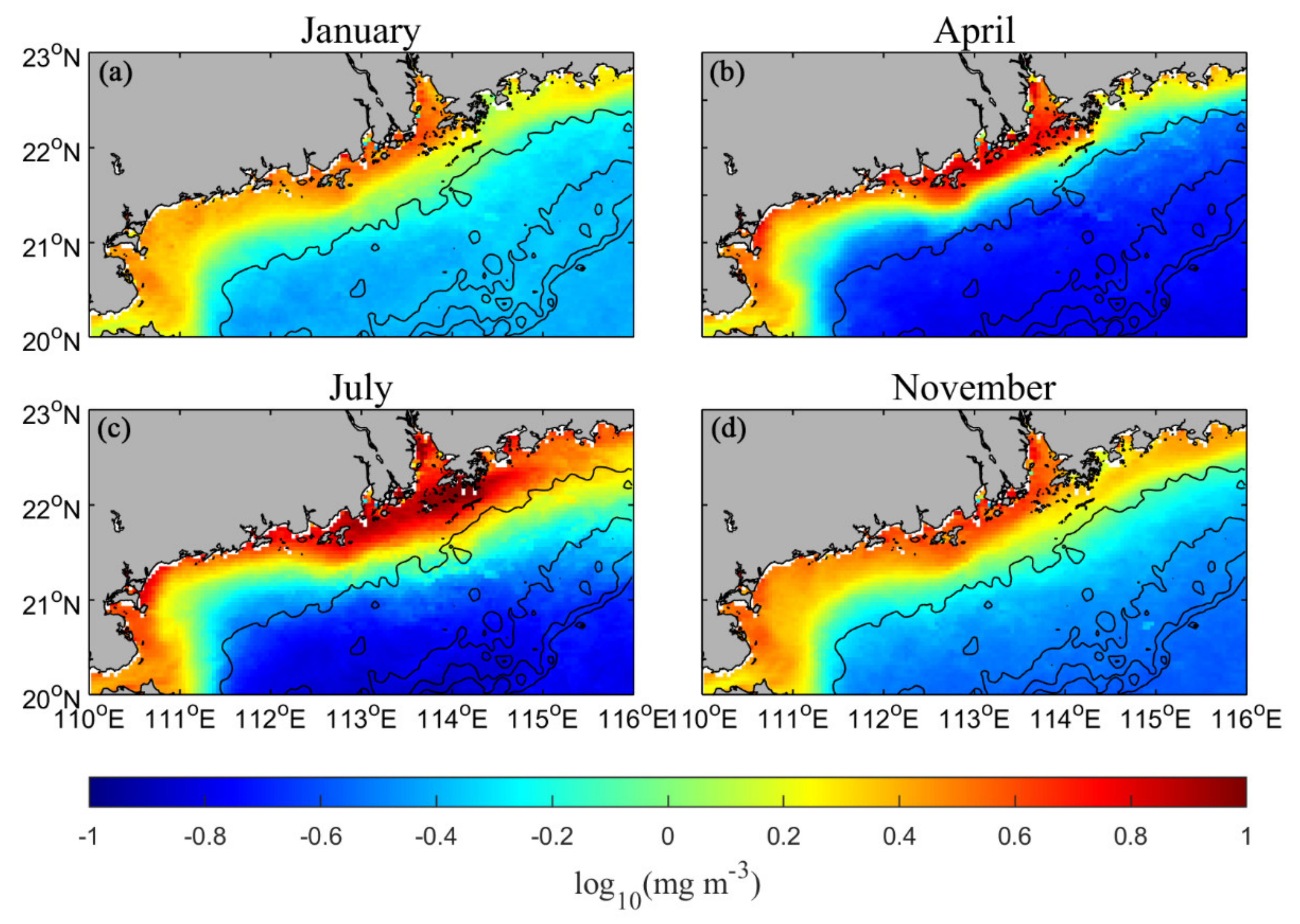
The area of high CHL also presents apparent seasonal variability (Figure 3). The concentrations of CHL to the west of the PR estuary are higher than those to the east of it in winter (Figure 3a). The feature maintains in spring, except for a larger increase in CHL in the PRP than in the far western coastal regions. This region of high CHL extends eastward to the east of the PRP in summer (Figure 3c), and the concentrations of CHL reach their annual maximum during this period. When it comes to autumn, the high CHL region shrinks back to the west of the PR estuary due to a large decrease in CHL to the east of the PR estuary.

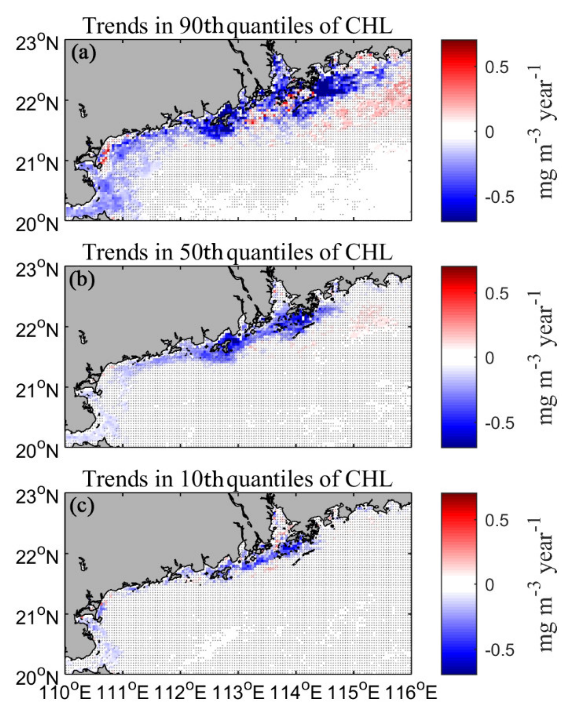
By employing quantile regression analysis on the time series of CHL at each 4 km grid across the NSCS, we mapped the spatial distributions of linear CHL trends in 90th, 50th, and 10th percentiles, and compared them with the trends in mean CHL values. The quantiles in the 90th, 50th, and 10th percentiles generally represent high, median and low CHL events, respectively. The results show noticeable negative trends in 90th percentiles along the northern coast of the NSCS (Figure 4a). The trends in this region are most apparent in the PRP (−0.1 mg m⁻³ year⁻¹) and least apparent to the east of the PR estuary (−0.02 mg m⁻³ year⁻¹). The area with noticeable trends narrows northeastward from approximately 80 km off the coast of Zhanjiang to approximately 40 km off the coast of Shanwei. A similar pattern is derived for quantile trends in 50th percentiles, but with much more moderate intensities (50% smaller than those in 90th percentiles). The trends in 50th percentiles are almost the same as those in mean CHL concentrations (Figure 4b,d). Noticeable negative trends in 10th percentiles are detected only in the PRP and east of Zhanjiang, with magnitudes smaller than those in 50th percentiles (Figure 4c). This difference suggests a more moderate decrease in low CHL events than that in mean values. In contrast, the greater negative trends in 90th percentiles indicate a larger decrease in high CHL events compared to that in mean values (Figure 4a,c). Taken together, these results suggest that not only the mean values but also the variance of CHL are decreased in the PRP during the past 21 years.

The differences in the variability of CHL between the PRP and the open NSCS are analyzed in detail by comparing the CHL trends in all quantiles, ranging from 5th to 95th percentiles in steps of 5%, between these two regions (represented by the regions in black boxes in Figure 4a). As demonstrated in Figure 5, negative trends are detected for all percentiles in the PRP, indicative of a decrease in CHL (for −0.04 mg m⁻³ year⁻¹ on average) during the past 21 years. The trends for different percentiles are not uniform, implying a change in the shape of CHL distribution. Specifically, the trends are similar (-0.04 ± 0.005 mg m⁻³ year⁻¹) for quantiles <50th, whereas the intensity of the trends enlarges dramatically to −0.06 mg m⁻³ year⁻¹ in 80th percentiles and <−0.07 mg m⁻³ year⁻¹ for quantiles >85th. The larger CHL decrease in high percentiles than in low percentiles indicates a decrease in the variance of the CHL. A negative trend of −0.05 mg m⁻³ year⁻¹ is derived by applying a linear regression on the CHL series. The trend is close to the quantile trend in 50th percentiles, which corresponds to the regression for the medians of the CHL series. In contrast, trends are of mixed signs for the series of CHL in the open NSCS regions. Although uniform negative trends are detected for quantiles <40th, the magnitudes of these trends (3–6 × 10⁻⁴ mg m⁻³ year⁻¹) are two orders of magnitude smaller than those of the trends in the PRP.

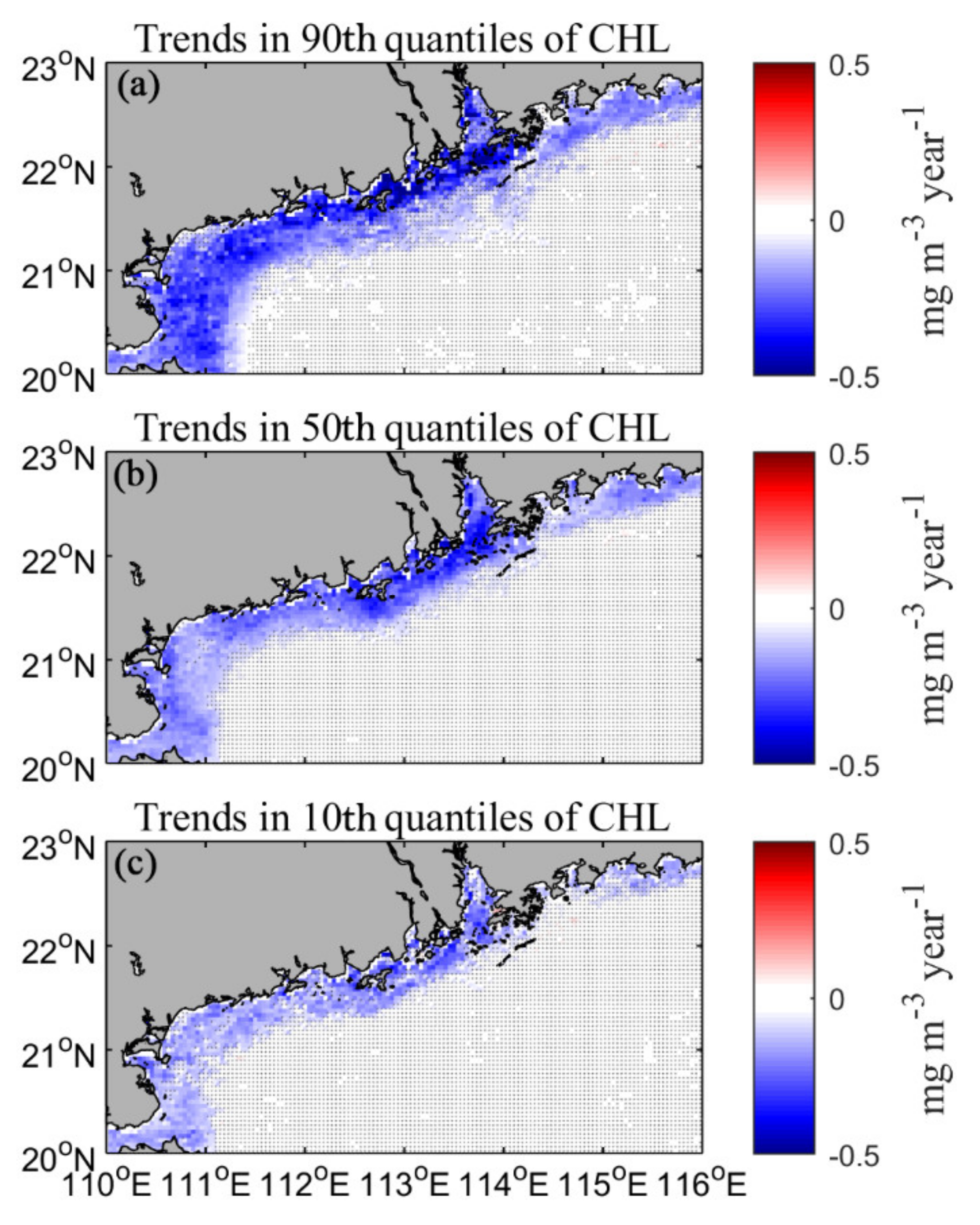
It is demonstrated in Figure 3 that the concentrations of CHL are high in summer and low in winter in the PRP. This means that the CHL trends in 90th percentiles may represent the variability of the high CHL in summer, while the trends in 10th percentiles represent the variability of the low CHL in winter. To better describe the long-term trends of CHL in different seasons, we applied the quantile regression analysis on the time series of CHL in summer (June, July, and August) and winter (December, January, and February), respectively. The results show negative trends in 90th percentiles along the coast in summer (Figure 6a). The magnitudes of the trends in the PRP are much larger than those in the eastern and western regions (−0.5 vs. −0.2 mg m⁻³ year⁻¹). The trends weaken with the decrease of quantiles from 90th to 10th percentiles (Figure 6). And the area of noticeable trends narrows to the PRP in 50th percentiles and only the PR estuary in 10th percentiles. These results suggest that the long-term decrease of the summertime CHL is restricted to the PRP, indicative of a close relation to the PR discharge.

The results are different for the quantile regression of wintertime CHL (Figure 7). Noticeable negative trends in 90th percentiles are detected in the entire coastal regions. The magnitudes of the trends to the east of the PR estuary (−0.3 mg m⁻³ year⁻¹) are smaller than those to the west of it (−0.2 mg m⁻³ year⁻¹). Similar patterns are derived for the trends in the 50th and 10th percentiles. The intensities of the trends in 90th percentiles are generally greater than those of the trends in 50th and 10th percentiles, indicative of a decrease in the variance of the CHL. Whereas, the differences in the CHL trends among the PRP, the western coasts, and the eastern coasts are not as apparent as the differences among them in summer.

4. Discussion

The high CHL in the PRP in summer is attributable to river discharge (Figure 3c). As presented by Harrison et al. [2], the PR discharge reaches its maximum in summer. The input of nutrients from the PR facilitates the growth of phytoplankton [46,47], thus leading to the concentrations of CHL being much higher than those in the western and eastern coastal regions. The seasonal migration of the high CHL patch in the PRP is possibly associated with the interactions between the monsoon and river discharge. During winter, the northeast monsoon produces shoreward Ekman transport, which promotes the westward spreading of terrestrial nutrients and facilitates the growth of phytoplankton [8], resulting in higher concentrations of CHL to the west than to the east of the PR estuary (Figure 3a). In contrast, the southwest monsoon produces offshore Ekman transport in summer [9,10]. The Ekman transport promotes the eastward spreading of terrestrial nutrients [5,11], thus resulting in the eastward extending of high CHL in the PRP (Figure 3c).

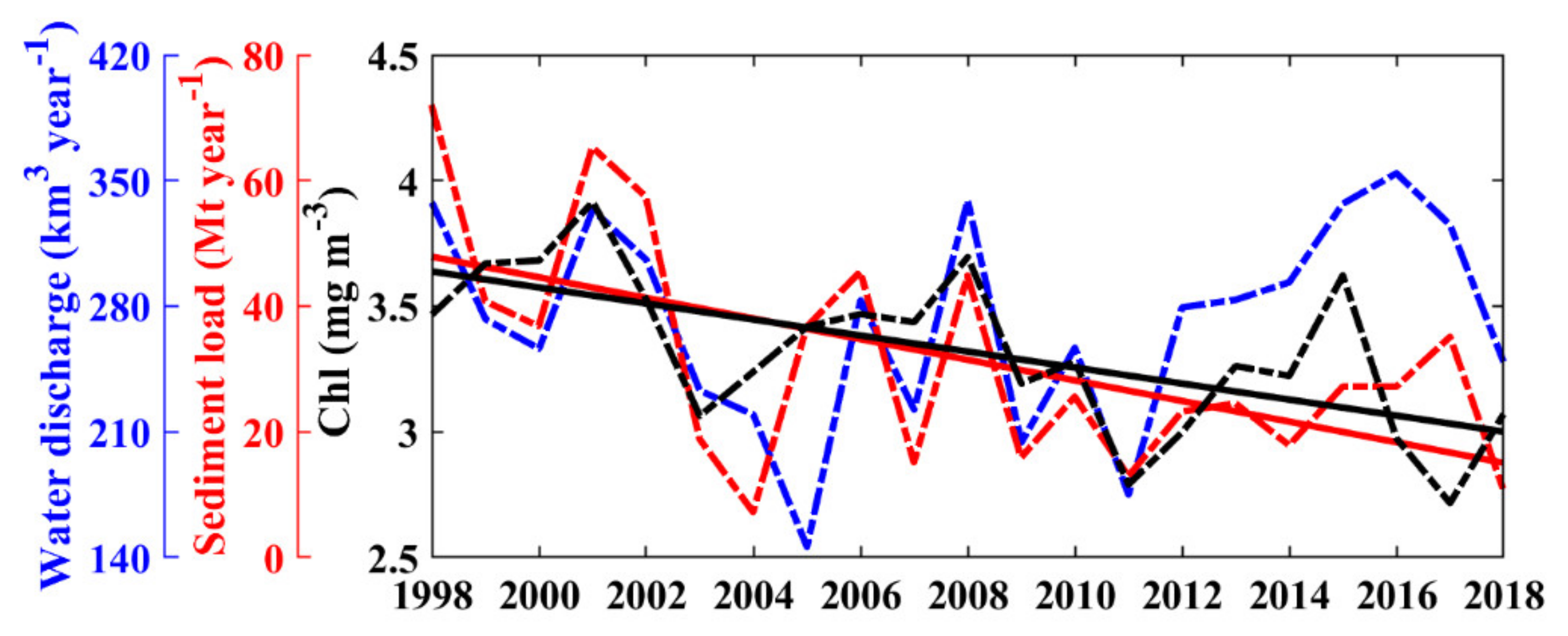
The decreasing trends of the CHL are most apparent in the PRP (Figure 4), especially in summer (Figure 6). This feature demonstrates the importance of river discharge in modulating the variability of the CHL. The amount of nutrients injected into the ocean is determined by the volume of river runoff and the content of nutrients in the water. Since we do not have long-term nutrients observations, we compared the annual variations of mean CHL in the PRP with those of mean PR water discharge and sediment load. The temporal variation of the CHL shows a positive correlation with that of the water discharge (R = 0.21, p = 0.36), especially before 2011 (R = 0.66, p <0.01) (Figure 8). Both the CHL and water discharge were increased in 2001, 2006, 2008, and 2010, and decreased in 2003, 2007, 2009, and 2011. After 2011, the water discharge increased to an extent much larger than the increase of the CHL. However, the sediment load did not increase apparently during this period, which suggests moderate changes in substances in the river water. The temporal variation of the CHL presents a high correlation (R = 0.56, p < 0.01) with that of the sediment load in the past 21 years. The decreasing trend of the CHL is also consistent with the decreasing of sediment load. As proposed by Liu et al. [1] and Zhan et al. [48], although the PR discharge did not show noticeable trends in the past decades, the sediment load decreased apparently in the past decades. Since both sediment and nutrients in the river originate from soil erosion, the decrease in the sediment may possibly imply a decrease in nutrients, which may be responsible for the decrease in the CHL.

It has been widely recognized that the variation of CHL in the SCS is influenced by wind forcing [49]. Numerous studies have demonstrated that wind-forced convective mixing alters the vertical flux of nutrients, thus modulates the growth of phytoplankton and the variation of CHL [19,49,50,51]. To determine the potential influence of wind on the decreasing trend of the CHL, we applied the same quantile regression analysis on weekly wind data from the WindSat between 2004 and 2019 (Figure 9). Considering the time length of the wind data is shorter than that of the CHL data, we checked the quantile trends of the CHL between 2004 and 2019. The results show similar trends to those between 1998 and 2019 (Figures not shown, could also be seen from the dashed black line in Figure 8). The resultant trends for median (as well as mean) wind speeds are negative (on average −0.05 m s⁻¹ year⁻¹) in the NSCS (Figure 9d,e). The intensities of the trends for quantiles >50th percentiles are greater than those for quantiles <50th percentiles. These features are in agreement with the large decreasing trends in high quantiles and small decreasing trends in low quantiles of the PRP CHL (Figure 5a,c). The decreasing trends of winds to the west of the PRP are higher than those to the east of it in 90th percentiles (Figure 9a). The pattern is consistent with the high decreasing trends of CHL to the west of the PRP (Figure 4a). The consistency in both spatial and temporal variability between the wind speeds and the CHL suggests that the weakening of winds may be a factor responsible for the decrease in CHL. As demonstrated by Zhang et al. [50], a weakening in wind indicates a decrease in convective mixing and vertical nutrient flux, thus a decrease in concentrations of phytoplankton and CHL. Whereas, the decrease in the wind is not significant in most regions for quantiles <50th percentiles (Figure 9c,e). This result suggests that the changes in moderate and low wind speeds may not be intense enough to induce apparent changes in CHL. The influence of wind might be secondary to that of the PR discharge.

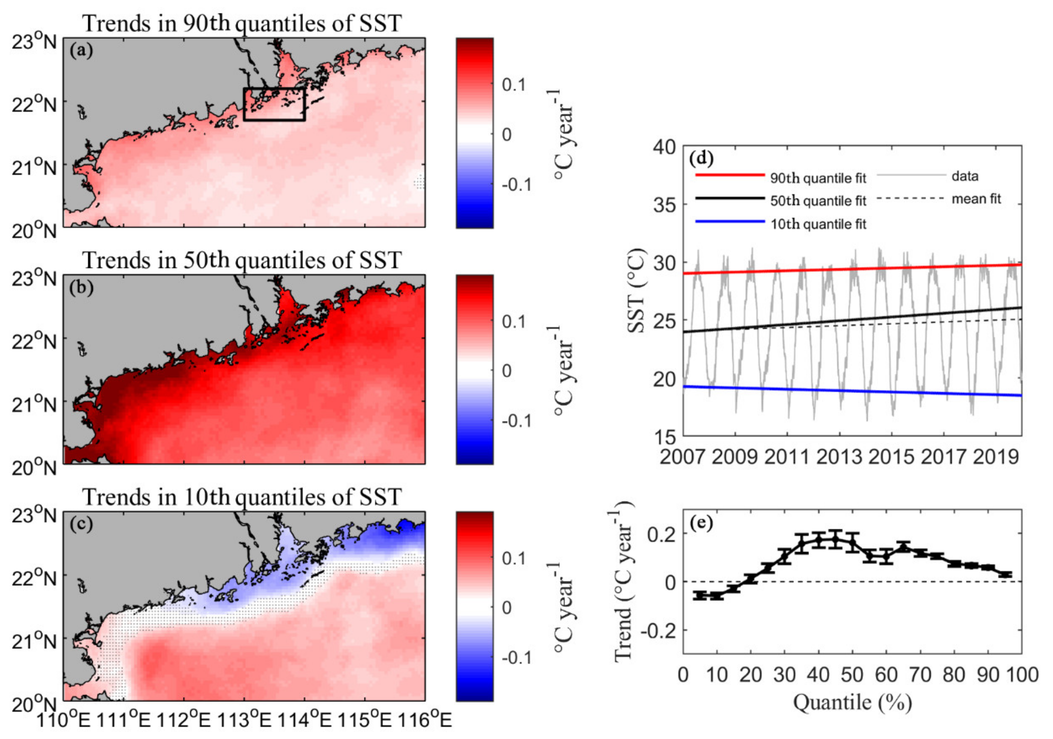
Sea surface temperature (SST) is also suggested to be able to modulate the variation of CHL. Recent studies suggested that the warming of the sea surface enhances the vertical stratification of the upper ocean, impedes the vertical flux of nutrients, and thus results in a decrease in CHL [21,52,53]. We mapped the trends for different quantiles of SST between 2007 and 2019 (Figure 10). During this period, the mean CHL in the PRP also presents a decreasing trend similar to that between 1998 and 2019 (dashed black line in Figure 8). In comparison, the trends of median (50th percentiles) and mean SST are positive (approximately 0.14 °C year⁻¹) (Figure 10d). Moreover, the SST trends in 50th percentiles are positive in the entire NSCS, with especially high values in the northwestern coast (Figure 10b). The feature is consistent with the large CHL decrease in 50th percentiles in the northwestern coast (Figure 4b). However, the SST trends in 90th percentiles are almost uniform in the entire NSCS (Figure 10a), contrasting to the intense spatial variability of the CHL trends (Figure 4a). The SST trends in 10th percentiles are negative in the PRP (Figure 10c), indicative of a decrease in SST and thus an increase in convective mixing, which is in contrast to the decrease in the CHL (Figure 4c). These results suggest that SST may not be a dominant factor responsible for the decrease in the CHL. Nevertheless, it is worthy to note that the annual mean SST was increased while annual low SST was decreased in the PRP during the past 13 years. The mechanisms and consequences for these changes are interesting questions that merit further investigation.

5. Conclusions

In summary, we applied the DINEOF to reconstruct the missing values in merged CHL data from multiple satellite observations between 1998 and 2018. The reconstructed data are complete in the spatial and temporal domain, apt for the analysis of the spatial and temporal variability of CHL. The resultant CHL images present high CHL values in the PRP, indicating the increase of productivity by the input of nutrients from the PR. The seasonality of the CHL in the PRP is markedly influenced by the seasonality of the river runoff. The PR discharge peaks in summer. During this period, the huge amount of terrestrial nutrients facilitate the growth of phytoplankton and increase the concentrations of CHL in the PRP. As a consequence, the CHL level is larger in summer than in winter, opposing to the seasonality of CHL in the open regions of the NSCS. The influence of the PR discharge on the CHL is modulated by the seasonally inverse monsoon. The northeast monsoon in winter promotes the westward spreading of PR water and results in high CHL to the west of the PR estuary. Whereas, the southwest monsoon in summer promotes the eastward extending of the PR water with high CHL. The quantile regression analysis on the CHL data reveals that both the mean values and the variance of the CHL in the PRP are decreased in the past 21 years. The CHL in this region decreases at a rate of 10⁻² mg m⁻³ year⁻¹, which is two orders of magnitudes greater than change rates of CHL in the open regions of the NSCS. The area with apparent decreasing trends is restricted to the PRP in summer and extends to the entire coastal region in winter. The decreasing trends in the CHL may be possibly attributed to the decrease in nutrient input from the river runoff and the weakening of wind-forced mixing. Whereas, the changes in SST do not appear to be a major factor responsible for the trends in the CHL.

References

- Liu, F.; Yang, Q.; Chen, S.; Luo, Z.; Yuan, F.; Wang, R. Temporal and spatial variability of sediment flux into the sea from the three largest rivers in China. J. Asian Earth Sci. 2014, 87, 102–115. [Google Scholar] [CrossRef]
- Harrison, P.J.; Yin, K.; Lee, J.H.W.; Gan, J.; Liu, H. Physical–biological coupling in the Pearl River Estuary. Cont. Shelf Res. 2008, 28, 1405–1415. [Google Scholar] [CrossRef]
- Zhai, W.; Dai, M.; Cai, W.-J.; Wang, Y.; Wang, Z. High partial pressure of CO2 and its maintaining mechanism in a subtropical estuary: The Pearl River estuary, China. Mar. Chem. 2005, 93, 21–32. [Google Scholar] [CrossRef]
- Liao, X.; Du, Y.; Wang, T.; Hu, S.; Zhan, H.; Liu, H.; Wu, G. High-Frequency Variations in Pearl River Plume Observed by Soil Moisture Active Passive Sea Surface Salinity. Remote Sens. 2020, 12, 563. [Google Scholar] [CrossRef] [Green Version]
- Gan, J.; Li, L.; Wang, D.; Guo, X. Interaction of a river plume with coastal upwelling in the northeastern South China Sea. Cont. Shelf Res. 2009, 29, 728–740. [Google Scholar] [CrossRef]
- Shu, Y.; Wang, D.; Zhu, J.; Peng, S. The 4-D structure of upwelling and Pearl River plume in the northern South China Sea during summer 2008 revealed by a data assimilation model. Ocean Model. 2011, 36, 228–241. [Google Scholar] [CrossRef]
- Ou, S.; Zhang, H.; Wang, D.-X. Dynamics of the buoyant plume off the Pearl River Estuary in summer. Environ. Fluid Mech. 2009, 9, 471–492. [Google Scholar] [CrossRef] [Green Version]
- Xue, H.; Chai, F. Coupled physical-biological model for the Pearl River Estuary: A phosphate limited subtropical ecosystem. In Estuarine and Coastal Modeling (2001); ASCE: Reston, VA, USA, 2002; pp. 913–928. [Google Scholar] [CrossRef] [Green Version]
- Chen, Z.; Pan, J.; Jiang, Y. Role of pulsed winds on detachment of low salinity water from the Pearl River Plume: Upwelling and mixing processes. J. Geophys. Res. Ocean. 2016, 121, 2769–2788. [Google Scholar] [CrossRef] [Green Version]
- Fong, D.A.; Geyer, W.R. Response of a river plume during an upwelling favorable wind event. J. Geophys. Res. Ocean. 2001, 106, 1067–1084. [Google Scholar] [CrossRef]
- Huang, B.; Lan, W.; Cao, Z.; Dai, M.; Huang, L.; Jiao, N.; Hong, H. Spatial and temporal distribution of nanoflagellates in the northern South China Sea. Hydrobiologia 2008, 605, 143–157. [Google Scholar] [CrossRef]
- Li, K.Z.; Yin, J.Q.; Huang, L.M.; Tan, Y.H. Spatial and temporal variations of mesozooplankton in the Pearl River estuary, China. Estuar. Coast. Shelf Sci. 2006, 67, 543–552. [Google Scholar] [CrossRef]
- Gan, J.; Lu, Z.; Dai, M.; Cheung, A.Y.Y.; Liu, H.; Harrison, P. Biological response to intensified upwelling and to a river plume in the northeastern South China Sea: A modeling study. J. Geophys. Res. 2010, 115. [Google Scholar] [CrossRef]
- He, X.; Xu, D.; Bai, Y.; Pan, D.; Chen, C.-T.A.; Chen, X.; Gong, F. Eddy-entrained Pearl River plume into the oligotrophic basin of the South China Sea. Cont. Shelf Res. 2016, 124, 117–124. [Google Scholar] [CrossRef]
- Zu, T.; Wang, D.; Gan, J.; Guan, W. On the role of wind and tide in generating variability of Pearl River plume during summer in a coupled wide estuary and shelf system. J. Mar. Syst. 2014, 136, 65–79. [Google Scholar] [CrossRef]
- Zhao, H.; Tang, D.; Wang, D. Phytoplankton blooms near the Pearl River Estuary induced by Typhoon Nuri. J. Geophys. Res. 2009, 114. [Google Scholar] [CrossRef]
- Boyce, D.G.; Lewis, M.R.; Worm, B. Global phytoplankton decline over the past century. Nature 2010, 466, 591–596. [Google Scholar] [CrossRef] [PubMed]
- Boyer, J.N.; Kelble, C.R.; Ortner, P.B.; Rudnick, D.T. Phytoplankton bloom status: Chlorophyll a biomass as an indicator of water quality condition in the southern estuaries of Florida, USA. Ecol. Indic. 2009, 9, S56–S67. [Google Scholar] [CrossRef]
- Palacz, A.P.; Xue, H.; Armbrecht, C.; Zhang, C.; Chai, F. Seasonal and inter-annual changes in the surface chlorophyll of the South China Sea. J. Geophys. Res. 2011, 116. [Google Scholar] [CrossRef]
- Liu, M.; Liu, X.; Ma, A.; Li, T.; Du, Z. Spatio-temporal stability and abnormality of chlorophyll-a in the Northern South China Sea during 2002–2012 from MODIS images using wavelet analysis. Cont. Shelf Res. 2014, 75, 15–27. [Google Scholar] [CrossRef]
- Shen, S.; Leptoukh, G.G.; Acker, J.G.; Yu, Z.; Kempler, S.J. Seasonal Variations of Chlorophyll Concentration in the Northern South China Sea. IEEE Geosci. Remote Sens. Lett. 2008, 5, 315–319. [Google Scholar] [CrossRef]
- He, Q.; Zhan, H.; Cai, S.; Li, Z. Eddy effects on surface chlorophyll in the northern South China Sea: Mechanism investigation and temporal variability analysis. Deep Sea Res. Part I Oceanogr. Res. Pap. 2016, 112, 25–36. [Google Scholar] [CrossRef]
- Gregg, W.W. Recent trends in global ocean chlorophyll. Geophys. Res. Lett. 2005, 32. [Google Scholar] [CrossRef] [Green Version]
- Boyce, D.G.; Dowd, M.; Lewis, M.R.; Worm, B. Estimating global chlorophyll changes over the past century. Prog. Oceanogr. 2014, 122, 163–173. [Google Scholar] [CrossRef]
- Barbosa, S.M. Quantile trends in Baltic sea level. Geophys. Res. Lett. 2008, 35. [Google Scholar] [CrossRef]
- Koenker, R.; Bassett, G., Jr. Regression quantiles. Econom. J. Econ. Soc. 1978, 46, 33–50. [Google Scholar] [CrossRef]
- Lee, K.; Baek, H.-J.; Cho, C. Analysis of changes in extreme temperatures using quantile regression. Asia-Pac. J. Atmos. Sci. 2013, 49, 313–323. [Google Scholar] [CrossRef]
- Gao, M.; Franzke, C.L.E. Quantile Regression–Based Spatiotemporal Analysis of Extreme Temperature Change in China. J Clim. 2017, 30, 9897–9914. [Google Scholar] [CrossRef]
- Franzke, C.L.E. Local trend disparities of European minimum and maximum temperature extremes. Geophys. Res. Lett. 2015, 42, 6479–6484. [Google Scholar] [CrossRef] [Green Version]
- McKinnon, K.A.; Rhines, A.; Tingley, M.P.; Huybers, P. The changing shape of Northern Hemisphere summer temperature distributions. J. Geophys. Res. Atmos. 2016, 121, 8849–8868. [Google Scholar] [CrossRef]
- Fan, L.; Chen, D. Trends in extreme precipitation indices across China detected using quantile regression. Atmos. Sci. Lett. 2016, 17, 400–406. [Google Scholar] [CrossRef] [Green Version]
- Tareghian, R.; Rasmussen, P. Analysis of Arctic and Antarctic sea ice extent using quantile regression. Int. J. Clim. 2013, 33, 1079–1086. [Google Scholar] [CrossRef]
- Maritorena, S.; D’Andon, O.H.F.; Mangin, A.; Siegel, D.A. Merged satellite ocean color data products using a bio-optical model: Characteristics, benefits and issues. Remote Sens. Environ. 2010, 114, 1791–1804. [Google Scholar] [CrossRef]
- Acker, J.G.; McMahon, E.; Shen, S.; Hearty, T.; Casey, N. Time-Series Analysis of Remotely-Sensed Seawifs Chlorophyll in River-Influenced Coastal Regions. 2009. Available online: https://ntrs.nasa.gov/search.jsp?R=20090042747 (accessed on 9 March 2020).
- Shang, S.; Dong, Q.; Hu, C.M.; Lin, G.; Li, Y.; Shang, S. On the consistency of MODIS chlorophyll a products in the northern South China Sea. Biogeosciences 2014, 11, 269. [Google Scholar] [CrossRef] [Green Version]
- Tang, D.; Kawamura, H.; Lee, M.-A.; Van Dien, T. Seasonal and spatial distribution of chlorophyll-a concentrations and water conditions in the Gulf of Tonkin, South China Sea. Remote Sens. Environ. 2003, 85, 475–483. [Google Scholar] [CrossRef]
- Beckers, J.-M.; Rixen, M. EOF calculations and data filling from incomplete oceanographic datasets. J. Atmos. Ocean. Technol. 2003, 20, 1839–1856. [Google Scholar] [CrossRef]
- Alvera-Azcárate, A.; Barth, A.; Rixen, M.; Beckers, J.M. Reconstruction of incomplete oceanographic data sets using empirical orthogonal functions: Application to the Adriatic Sea surface temperature. Ocean Model. 2005, 9, 325–346. [Google Scholar] [CrossRef] [Green Version]
- Hilborn, A.; Costa, M. Applications of DINEOF to Satellite-Derived Chlorophyll-a from a Productive Coastal Region. Remote Sens. 2018, 10, 1449. [Google Scholar] [CrossRef] [Green Version]
- Miles, T.N.; He, R. Temporal and spatial variability of Chl-a and SST on the South Atlantic Bight: Revisiting with cloud-free reconstructions of MODIS satellite imagery. Cont. Shelf Res. 2010, 30, 1951–1962. [Google Scholar] [CrossRef]
- Ji, C.; Zhang, Y.; Cheng, Q.; Tsou, J.; Jiang, T.; Liang, X.S. Evaluating the impact of sea surface temperature (SST) on spatial distribution of chlorophyll-a concentration in the East China Sea. Int. J. Appl. Earth Obs. Geoinf. 2018, 68, 252–261. [Google Scholar] [CrossRef]
- Wang, Y.; Liu, D. Reconstruction of satellite chlorophyll-a data using a modified DINEOF method: A case study in the Bohai and Yellow seas, China. Int. J. Remote Sens. 2013, 35, 204–217. [Google Scholar] [CrossRef]
- Alvera-Azcárate, A.; Vanhellemont, Q.; Ruddick, K.; Barth, A.; Beckers, J.-M. Analysis of high frequency geostationary ocean colour data using DINEOF. Estuar. Coast. Shelf Sci. 2015, 159, 28–36. [Google Scholar] [CrossRef] [Green Version]
- Koenker, R.; Hallock, K.F. Quantile regression. J. Econ. Perspect. 2001, 15, 143–156. [Google Scholar] [CrossRef]
- Fan, L. Quantile trends in temperature extremes in China. Atmos. Ocean. Sci. Lett. 2014, 7, 304–308. [Google Scholar]
- Li, J.; Jiang, X.; Jing, Z.; Li, G.; Chen, Z.; Zhou, L.; Zhao, C.; Liu, J.; Tan, Y. Spatial and seasonal distributions of bacterioplankton in the Pearl River Estuary: The combined effects of riverine inputs, temperature, and phytoplankton. Mar. Pollut. Bull. 2017, 125, 199–207. [Google Scholar] [CrossRef] [PubMed]
- Lee Chen, Y.-l.; Chen, H.-Y. Seasonal dynamics of primary and new production in the northern South China Sea: The significance of river discharge and nutrient advection. Deep Sea Res. Part I Oceanogr. Res. Pap. 2006, 53, 971–986. [Google Scholar] [CrossRef]
- Zhan, W.; Wu, J.; Wei, X.; Tang, S.; Zhan, H. Quantile trend analysis for suspended sediment concentration in the Pearl River Estuary based on remote sensing. J. Trop. Oceanogr. 2019, 38, 32–42. [Google Scholar] [CrossRef]
- Liu, K.K.; Wang, L.W.; Dai, M.; Tseng, C.M.; Yang, Y.; Sui, C.H.; Oey, L.; Tseng, K.Y.; Huang, S.M. Inter-annual variation of chlorophyll in the northern South China Sea observed at the SEATS Station and its asymmetric responses to climate oscillation. Biogeosciences 2013, 10, 7449–7462. [Google Scholar] [CrossRef] [Green Version]
- Zhang, W.; Wang, H.; Chai, F.; Qiu, G. Physical drivers of chlorophyll variability in the open South China Sea. J. Geophys. Res. Oceans 2016, 121, 7123–7140. [Google Scholar] [CrossRef]
- Xian, T.; Sun, L.; Yang, Y.J.; Fu, Y.F. Monsoon and eddy forcing of chlorophyll-a variation in the northeast South China Sea. Int. J. Remote Sens. 2012, 33, 7431–7443. [Google Scholar] [CrossRef]
- Duan, R.; Yang, K.; Ma, Y.; Hu, T. A study of the mixed layer of the South China Sea based on the multiple linear regression. Acta Oceanol. Sin. 2012, 31, 19–31. [Google Scholar] [CrossRef]
- Tang, S.; Liu, F.; Chen, C. Seasonal and intraseasonal variability of surface chlorophyll a concentration in the South China Sea. Aquat. Ecosyst. Health Manag. 2014, 17, 242–251. [Google Scholar] [CrossRef]
Figure 1.
(a) Geographic distributions of climatological mean concentrations of near-surface chlorophyll-a (CHL) in the northern South China Sea (NSCS) (between 1998 and 2018). (b) Months when the concentrations of CHL reach the maximum. (c) and (d) Climatological monthly averages (lines) and corresponding standard deviations (shadings) of CHL in the Pearl River Plume (PRP) (113° E–114° E, 21.7° N–22.2° N) and open regions of the NSCS (113° E–114° E, 20.2° N–20.7° N) (black boxes in (a)). The black contours in (a) are isobaths with an interval of 50 m.
Figure 2.
Comparison of CHL data from single satellites (top, left to right are data from Sea-viewing Wide Field-of-view Sensor (SeaWiFS), Moderate Resolution Imaging Spectroradiometer (MODIS) and Medium Resolution Imaging Spectrometer (MERIS), respectively), the merged data from the GlobColour (middle) and the reconstructed data by the Data Interpolating Empirical Orthogonal Functions (DINEOF) (bottom).
Figure 3.
Climatological averages of CHL in (a) January, (b) April, (c) July, and (d) November (between 1998 and 2019). The black contours are isobaths as defined in Figure 1a.
Figure 4.
Geographic distributions of quantile regression trends in (a) 90th, (b) 50th, and (c) 10th percentages of CHL between 1998 and 2019. (d) presents the linear trends of mean CHL. The black boxes are the PRP and open NSCS regions, as in Figure 1. The superposed stippling show areas where the trends are not significant at a 5% level.
Figure 5.
Time series of mean CHL (gray) and CHL trends in quantiles of 90th (red), 50th (black), and 10th (blue) in (a) the PRP and (b) the open NSCS (black boxes in Figure 4a) between 1998 and 2019. The black dashed lines denote the linear regression of the mean CHL. (c) and (d) present the corresponding trends (slopes) in all quantiles ranging from 5th to 95th percentages in steps of 5%. The vertical bars are standard errors in each regression.
Figure 6.
Geographic distributions of quantile regression trends in (a) 90th, (b) 50th, and (c) 10th percentages of CHL in summer (June, July, and August) between 1998 and 2019. The superposed stippling show areas where the trends are not significant at a 5% level.
Figure 7.
Geographic distributions of quantile regression trends in (a) 90th, (b) 50th, and (c) 10th percentages of CHL in winter (December, January, and February) between 1998 and 2019. The superposed stippling show areas where the trends are not significant at a 5% level.
Figure 8.
Annual variations of Pearl River (PR) discharge (dashed blue line), sediment load (dashed red line) and mean CHL in the PRP (dashed black line). The solid black and red lines are linear regressions of the time series of the CHL and sediment load, respectively.
Figure 9.
Geographic distributions of quantile regression trends in (a) 90th, (b) 50th, and (c) 10th percentages of wind speeds between 2004 and 2019. The superposed stippling show areas where the trends are not significant at a 5% level. (d) Time series of mean wind speed (gray) and trends of the wind speeds in quantiles of 90th (red), 50th (black) and 10th (blue) in the NSCS. The black dashed line denotes the linear regression of the mean wind speeds. (e) Slopes of the trends of the wind speeds in (d) for all quantiles ranging from 5th to 95th percentages in steps of 5%. The vertical bars are standard errors in each regression. Note that since the wind data is not available near the coast, the plots in (d) and (e) are based on the series of mean wind speed in the entire region in (a).
Figure 10.
Geographic distributions of quantile regression trends in (a) 90th, (b) 50th, and (c) 10th percentages of sea surface temperature (SST) between 2007 and 2019. The superposed stippling show areas where the trends are not significant at a 5% level. (d) Time series of mean SST (gray) and trends of the SSTs in quantiles of 90th (red), 50th (black), and 10th (blue) in the PRP (black box in (a)). The black dashed line denotes the linear regression of the mean SSTs. (e) Slopes of the trends of the SSTs in (d) for all quantiles ranging from 5th to 95th percentages in steps of 5%. The vertical bars are standard errors in each regression.
© 2020 by the authors. Licensee MDPI, Basel, Switzerland. This article is an open access article distributed under the terms and conditions of the Creative Commons Attribution (CC BY) license (http://creativecommons.org/licenses/by/4.0/).
Share and Cite
MDPI and ACS Style
Gao, N.; Ma, Y.; Zhao, M.; Zhang, L.; Zhan, H.; Cai, S.; He, Q. Quantile Analysis of Long-Term Trends of Near-Surface Chlorophyll-a in the Pearl River Plume. Water 2020, 12, 1662. https://0-doi-org.brum.beds.ac.uk/10.3390/w12061662
AMA Style
Gao N, Ma Y, Zhao M, Zhang L, Zhan H, Cai S, He Q. Quantile Analysis of Long-Term Trends of Near-Surface Chlorophyll-a in the Pearl River Plume. Water. 2020; 12(6):1662. https://0-doi-org.brum.beds.ac.uk/10.3390/w12061662
Chicago/Turabian StyleGao, Na, Yi Ma, Mingli Zhao, Li Zhang, Haigang Zhan, Shuqun Cai, and Qingyou He. 2020. "Quantile Analysis of Long-Term Trends of Near-Surface Chlorophyll-a in the Pearl River Plume" Water 12, no. 6: 1662. https://0-doi-org.brum.beds.ac.uk/10.3390/w12061662
Note that from the first issue of 2016, this journal uses article numbers instead of page numbers. See further details here.