
Fragility Curves for Slope Stability of Geogrid Reinforced River Levees


Faculty of Civil Engineering, University of Zagreb, 10000 Zagreb, Croatia
*
Author to whom correspondence should be addressed.
Water 2021, 13(19), 2615; https://0-doi-org.brum.beds.ac.uk/10.3390/w13192615
Submission received: 9 September 2021
/
Revised: 15 September 2021
/
Accepted: 16 September 2021
/
Published: 23 September 2021
(This article belongs to the Special Issue Dam Safety. Overtopping and Geostructural Risks)
Abstract
:When constructing flood protection structures such as river levees, oftentimes due to various factors engineers must design composite structures, i.e., reinforced earthen structures which comply with all the stability criteria. The most common way of reinforcing such structures is the usage of geosynthetics, or mostly geogrids when talking about stability. Since geosynthetics are man-made materials produced in a controlled environment and go through quality control measures, their characteristics contain a negligible amount of uncertainty compared to natural soils. However, geosynthetic handling, their installation in the levee, and their long-term degradation can all have significant effects of variable magnitude on geosynthetic characteristics. These effects and their variability can be considered as random variables, which can then be used in probabilistic analyses together with soil properties. To investigate the effects of the geogrid’s resistance variability on slope stability compared to soil properties variability, probabilistic analyses are conducted on a river levee in northern Croatia. It is found that the geogrid’s variability generally has very little effect on the total uncertainty compared to the friction angle’s variability, but out of the three geogrid layers used the top grid has the most influence.
1. Introduction
River levees for flood protection are structures usually made from earthfill material, and their cross section can be made up of multiple distinct parts, which serve specific purposes in the protection from high waters. However, as Wang et al. [1] noted, levees cannot completely exclude flood disasters, and living behind a levee poses unique flood risks since levees are designed to reduce the impact of a flood event at a certain scale.
Their stability is mostly affected by the material used for the levee body, the foundation material, and is also a function of the water level on the riverside. Often, due to cadastral parcels owned by the investor, stability cannot be ensured for required crown heights corresponding to defined return periods of flood events by using conventional solutions due to the need of building steep slopes to fit the levee into the parcel width. This issue is commonly solved by introducing ground reinforcement techniques that allow for steeper slopes. One common technique in such structures is the reinforced fill built by placing geosynthetic layers during the construction or reconstruction of a levee. The use of geosynthetic materials generally in reinforced earth structures started to increase after 1971 when the first geotextile reinforced wall was constructed in France, and their beneficial effect was noticed. At a later date, around 1980, geogrids were developed [2]. Nowadays, geosynthetics are widely used in various fields of geotechnical engineering, such as shallow footing to increase bearing capacity and decrease settlement [3,4,5], retaining walls [6,7,8], and road construction [9,10]. When used in levees, their benefit has also been shown in decreasing settlement of levees on soft soil [11] and increasing slope stability [12], or both. Their effects have been studied under undrained [13,14], partially drained [14], and drained [15] conditions, during and after embankment construction. Hird and Kwok [13] studied the stress distribution in the geosynthetic element depending on its stiffness, and the strength and stiffness of the embankment material. As the levees can be made from various materials, Balakrishnan and Viswanadham [16] studied the tensile load-strain behaviour of geogrids embedded in different soil types and under variable normal stress. Other ground reinforcement methods can also be combined with geosynthetics. For example, Zheng et al. [17] have used stone columns in conjunction with geosynthetics to achieve stable embankments on soft soil and have studied their interaction.
Studies have shown the stability benefit of using geosynthetics to ensure embankment stability, as well as the economic advantages, with the help of limit equilibrium based methods [18,19,20] and numerical methods [14,21,22] in 2D and 3D [23], physical models [24], as well as various other methods mentioned by Tandjiria et al. [25]. In practice, the most used method is the limit equilibrium due to its simplicity, despite all the limitations and assumptions, which has shown good performance in real-life problems [25].
The introduction of geosynthetics for stability, mostly geogrids, is significant not only because it means a higher stability, but also because it is a reinforcement element which can be made from various materials (polyester, polypropylene, polyethylene, polyamide, polyester, and polyvinyl chloride) [26], and whose characteristics can be controlled during their production, which in turn means a higher reliability in their parameters’ values and less variability. Nevertheless, some variability within geogrid parameters can still arise from various sources, namely biases regarding strength reduction factors, which consider installation damage, creep, and durability.
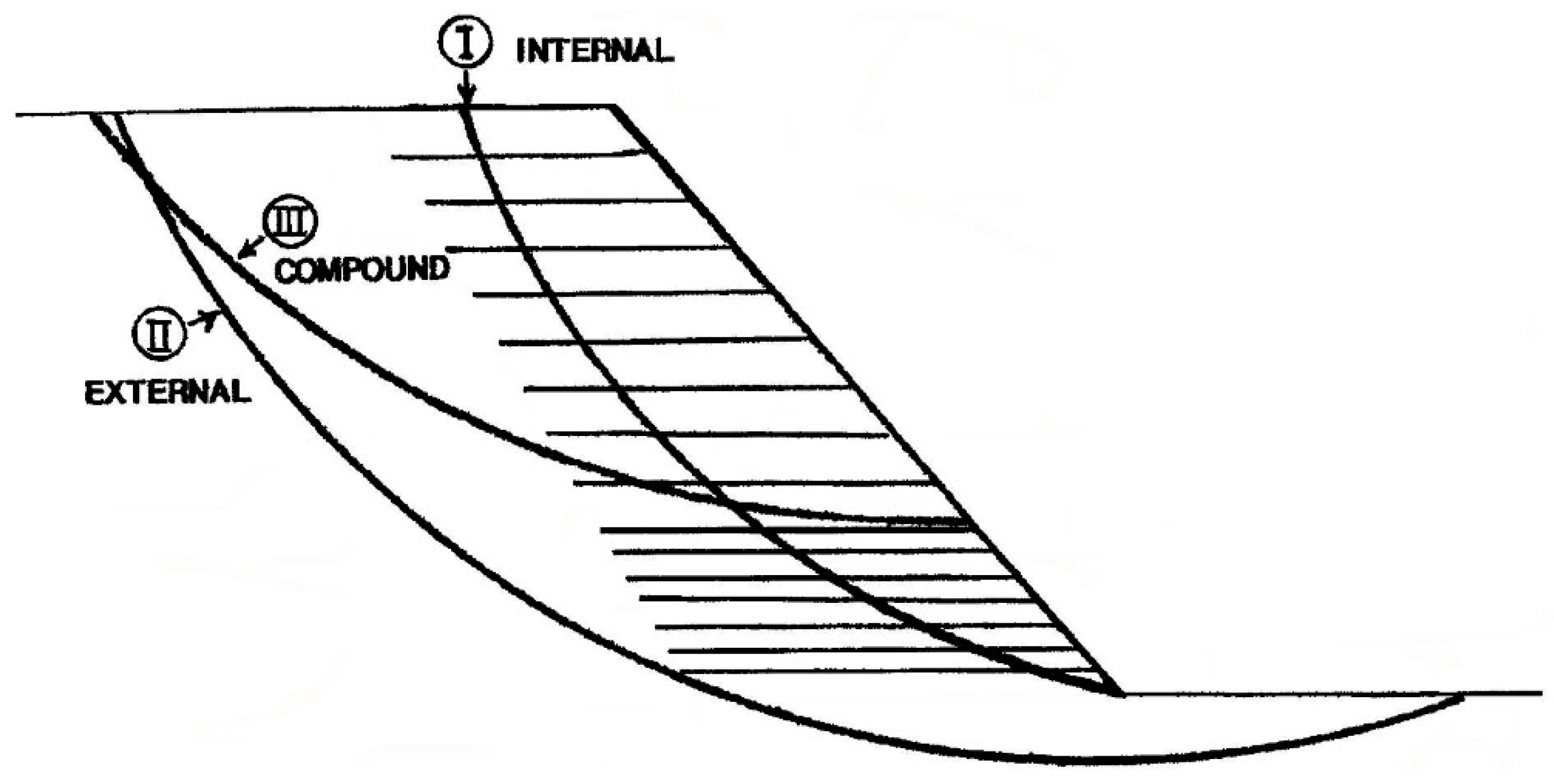
As Rowe and Soderman [18] stated, geosynthetics can fail by two mechanisms, either on the soil-reinforcement interface, or internally as the rupture of the reinforcement element itself. To resist the tensile rupture of the element, the resistance is straightforwardly calculated by using the material’s parameters and the cross section. To resist pull out, multiple effects are in place, whose relative contribution to the total pull-out resistance effect has been studied by various authors [24,27,28]. When such elements are placed within a levee, a few failure modes can be expected, namely internal, external, and compound [29], as shown in Figure 1. Internal stability refers to slip surfaces which pass entirely through the reinforcement layers, which means that the reinforcement failed either by tensile rupture, or by pull out. External failure refers to deeper slip surfaces which go around all the reinforcement layers. The compound failure is the most common type, where the slip surface goes around and through various reinforcement layers. On top of those mentioned failure modes, if the spacing between neighbouring reinforcement layers is too big and secondary reinforcement is not provided, failure can initiate by soil sliding between those layers, which then leads to a global failure. Thus, geogrid reinforced slope sections usually consist of primary or principal, and secondary or intermediate, geogrid layers [2,29,30,31]. Failure of the slope can also occur without the need of reinforcement failure, i.e., if the reinforcement is a low stiffness geosynthetic whose failure strain is much larger than the strain at which the slope fails, then the whole slope might fail without reaching any of the previously defined geosynthetic failure mechanisms [18]. Which failure mechanism will occur in a levee highly depends on the cross section of the levee and whether it is a newly constructed levee or a reconstructed one, because these parameters will dictate the placement of geogrids.
Even though levees are characterized by a number of failure mechanisms [32,33], and that about half of earth embankment failures occur as a result of processes related to piping [34], this study considers only the slope stability of a reconstructed and additionally reinforced river levee. The primary purpose of this study is to investigate the sensitivity of reinforced levees to rising water levels and uncertainties in geotechnical materials, while also promoting the usage of probabilistic analyses which can take those uncertainties into consideration. Thus, probabilistic analyses are conducted with the objective of quantifying the effects of uncertainties related to geogrid reinforcement on the slope stability of levees, and to construct fragility curves which show the probability of failure of the levee for any water level. Such probabilistic slope stability analyses can be conducted using numerous methods [35,36,37,38,39,40,41,42,43]. In this study, the limit equilibrium method is adopted due to its simplicity and wide usage in geotechnical practice, while results are further processed with programmed probabilistic methods to find the probabilities of unwanted behavior of the levee subjected to various water levels with steady state conditions. The statistical techniques and probabilistic methods used in this study are the Surface Response Method (SRM) and the First Order Reliability Method (FORM), which have been programmed with MATLAB. The variability values of random variables used for probabilistic calculations are selected as reported in literature. Since the considered sources of variability of geogrids include the long-term degradation, and no seismic event is considered, the conditions considered for the whole levee are drained. The case study is described in Section 3.
Fragility curves, which will be constructed as a result of this study, are curves showing the conditional probability of an unwanted behaviour occurring as a result of increasing the design event intensity. Their usage in civil engineering began in, at least, 1980 with the work of Kennedy et al. [44] related to the safety of a nuclear power plant. Later, their usage in flood protection started in 1991 with a USACE Policy Guidance Memorandum [45], followed by a further explanation in a 1993 USACE Engineer Technical Letter [46], as reported by [47]. Today, their usage in slope stability is widespread [35,39,47], with regards to seismic events, rainfall, and rising water level.
2. Methodology
In this study, the Hasofer-Lind method is employed [48], also known as the First Order Reliability Method (FORM), together with the surface response method (SRM) for approximatively calculating the reliability of the flood protection embankment. The SRM is a statistical technique used to approximate the response of a model to input variables by using a suitable function when the true relationship is unknown. The approximation is done by fitting the selected function to the original model evaluated at multiple sample points, i.e., the coefficients of the function are determined by an error minimization technique. It is chosen as a relatively simple tool to complement the FORM by defining the required performance function. In this study it is used to construct an n-dimensional surface which approximates the response of the levee, where n is the number of random variables, based on known function values and on regression analysis. The surface used in this study is a quadratic function defined by a second-order polynomial, as shown in Equation (4). The coefficients of the function are obtained by minimizing the error between the original and approximated functions [49]. After that, the probability of failure is obtained through FORM optimization. The FORM is an upgrade to the First Order Second Moment (FOSM) method with its geometrical interpretation of the reliability index, which is invariant to the performance function format. To employ it, the first step is to convert all random variables to independent variables in the standard normal space with zero mean and unit standard deviation, and the performance function needs to be known. It offers a solution which defines the reliability index () as the shortest distance from the failure function (defined by SRM and the performance function) to the origin of the standard variable space, which is the mean of the joint probability distribution, and is the most efficient method for estimating for problems involving one dominant failure mode [50]. Rackwitz [51] noted that, for 90% of all application, the FORM fulfils all practical needs, and its numerical accuracy is usually more than sufficient. Since all the random variables are normally distributed and independent, the transformation to the standard normal space is simply done by Equation (1) [52].
where is the standard normal variable value, μ the mean value of the original variable, and σ the standard deviation of the original variable.
The first step in the analyses is to determine the number of random variables to be used, and their respective statistics. The mechanisms of failure of the geogrids are the rupture of the elements, or the pull out of the grid from the soil. Regarding the tensile strength, as there are three rows of geogrids reinforcing the body, the ultimate tensile strength of each of them is simulated as an independent random variable. The interaction between reinforcement and soil depends on various factors, including grid parameters such as roughness, grid opening dimensions, thickness of transverse ribs and deformability characteristics, as well as soil parameters such as friction angle, grain size distribution, particle shape, density, water content, cohesion, and stiffness [2]. For the pull-out parameters in this study, the soil-grid interface friction is taken as a fraction of the soil internal friction angle, while the cohesion is ignored. As the soil-grid interface friction depends on the friction angle of the material which covers the grid, the internal friction angle of that material is also taken as a random variable. Thus, a total of 4 random variables are considered (Table 3). Since there is no face anchorage, the sliding of the soil on the soil-grid interface can happen on either end of the grid, i.e., inside the body or at the face. Throughout the analyses, a specific soil-grid friction ratio is kept constant to investigate the behaviour at various ratios. The analyses are performed for three design cases with different interface friction, named here as SIF (small interface friction), MIF (mean interface friction) and HIF (high interface friction). Sia and Dixon [53] analysed the variability of interface strength parameters between soil and geotextiles or geomembranes in coarse- and fine-grained soils. In this paper, the ratio is held constant as a deterministic parameter. For the MIF case, a contact friction angle of 2/3 φ is used, which is the recommended conservative value for geosynthetics [2]. This is closely in agreement with values obtained by Yu and Bathurst [54] who used a reduction factor applied to the tangent of backfill friction angle of 0.5–0.8, with the best agreement between pull out tests and numerical model results being 0.67 or 2/3. Other studies propose different values, e.g., Ferreira et al. [12] define the interface friction angle as 6/7 φ, while Jewell [55] takes a factor of 0.8 as the “direct sliding coefficient” as a value to “safely encompass most practical cases”. In this study, the factor 0.67 is used as the mean value but applied directly to the friction angle instead of its tangent (which is equivalent to applying a factor of 0.63 to the tangent). For the other two cases, SIF and HIF, interface friction ratios of 0.5 and 1 are used, respectively.
Next, an arbitrary number of different deterministic slope stability analyses are conducted for each water level by varying the random variables’ values. In this study, this is achieved with the help of Latin Hypercube simulations, which varied the grids’ strength for each chosen friction angle. All the variables’ values are then transformed into the standard normal variable space by Equation (1), and the resulting safety factor is corrected accordingly with the appropriate performance function, as follows. The performance function is defined for two cases and shown in Equations (2) and (3), one for failure condition where FS = 1 (ULS), and one for an arbitrary safety factor value of FS = 1.5. The “probability of failure” calculated for the second case actually refers to the probability of reaching the defined threshold. When the performance functions defined by the left and middle terms in Equations (2) and (3) are equated to zero, this becomes the limit state function which defines failure or unwanted behaviour. Deterministic slope stability analyses, as well as steady seepage analyses, are conducted using Slide2 v9.009, Rocscience Inc., Toronto, ON, Canada.
Such defined groups consisting of standard normal variables’ values and the respective performance function values for each water level are fitted with a polynomial shown in Equation (4) [56].
The symbolizes an approximation of the real performance function, where “c”, “b”, and “a” are its coefficients, N is the number of random variables, and “x” the random variables’ values. The fitting is done in MATLAB by minimizing the sum of squared residuals with the lsqcurvefit function, where the value or the performance function and the random variables are known. The results of such minimization are the coefficients “c”, “b”, and “a” for a polynomial, which approximates the performance function in the vicinity of the design point (1 or 1.5). Now that the coefficients are known, a constrained optimization (minimization) is run. What we are searching for is the minimal value of the Euclidean norm of the standard normal variables which satisfies the condition that . This is done by minimizing the vector of standard normal variables with the constraint , by using the MATLAB function fmincon.
The result is, (1) the reliability index β defined as the shortest value of the radius vector xi which defines the limit state function, and (2) the standard normal variables’ values xi which give the previously defined distance. After a few iterations, these values converge towards the true limit state function. When the difference between two iterations becomes negligible, the procedure stops. This is usually achieved within 2–4 iterations for this study. Each iteration contains new deterministic slope stability analyses with new random variables’ values, which resulted from previous iterations. To calculate the probability of failure from the resulting reliability index, the cumulative standard normal distribution is calculated for the reliability index with inversed sign. As the optimization needs a set of starting values, they are varied for the same calculation to check for the robustness of the result and for local minima. Another quality check is made by plotting surfaces in a 3-dimensional space by ignoring 2 of the random variables. To accept the result, not only is a small change in consecutive iterations needed, but also the quality of regression between the real performance function and the approximated one, as shown in Equation (6) [56], needs to be ≥0.95.
where is the expected value of the performance function, simply taken as the arithmetic mean of all the deterministic performance function values. On top of that, the mean square error (MSE) is also calculated by Equation (7), and the results varied between 5 × 10⁻⁶ and 2 × 10⁻¹⁹.
The whole process is repeated for various water levels, and fragility curves are constructed.
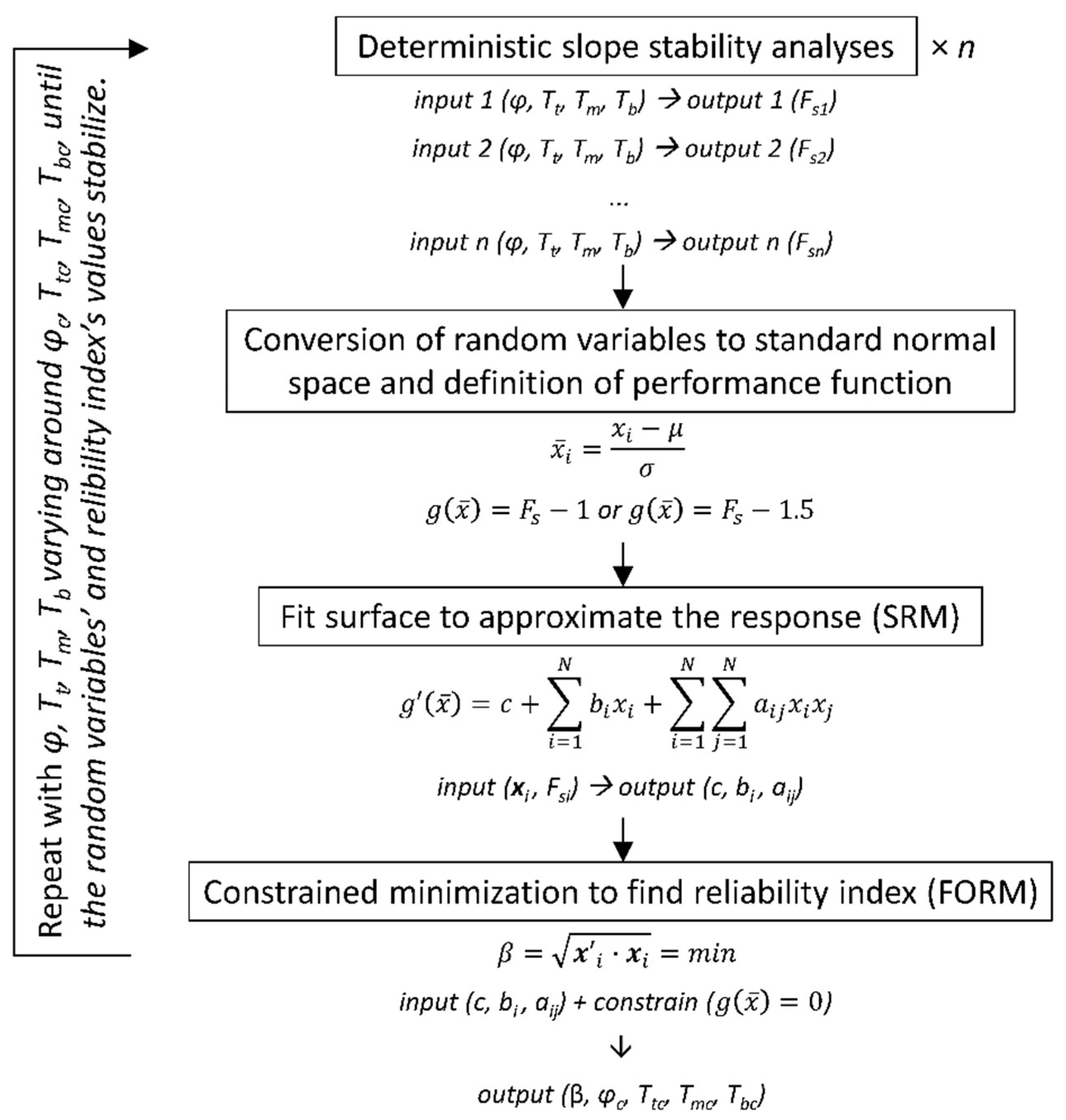
The previously discussed methodology for the development of fragility curves for levee stability, summarized in Figure 2, requires the proper water pressure state to be established. For the design situations which include water level up to the top of levee crown, numerical analyses include commonly used boundary conditions of properly defined hydraulic heads on the riverside and landside. However, as Librić et al. [57] found in their study, the overtopping of the case study levee has a high risk exposure compared to other risks, thus overflow is also considered in this study. Overtopping (i.e., overflow) is usually a result of a high-water event (surge), or it can occur due to wave overtopping. The combined effect of surge and wave overflow is discussed by many authors [58,59,60]. However, for the river levee considered, only a surge type of overflow is relevant. When the water level rises higher than the crown, the stress analyses are supplemented with the additional boundary shear stress along the crown and landside slope. Additionally, a trapezoidal stress is applied over the crown during overflow to simulate water pressure, corresponding to the height of water on the upstream side, and to the water height on the downstream side calculated by Equation (10). Given that this aspect goes beyond standard analyses, a cautious evaluation of these shear stresses is required. The boundaries of both analyses are defined far from the levee region, enough to not affect the results. Seepage analyses require only hydraulic boundary conditions, which in this case consist of constant or varying hydraulic head values applied on lateral boundaries and on the top boundary of the model, up to the required height. During surge overflow, the water velocity increases down the slope until a terminal velocity is reached at equilibrium between water momentum and slope frictional resistance, after which the flow becomes steady and the velocity can be calculated by the following equation:
where v0 (m/s) is the steady flow velocity, θ (°) is the landside slope angle, n (-) is the Manning’s coefficient, and q0 (m2/s) is the steady discharge [58]. For supercritical flow, which develops on the landside slope—as shown in Figure 3—Hewlett et al. [61] proposed a value of Manning’s coefficient of n = 0.02, relevant for slopes of 1:3.
The discharge over the levee crown can be calculated using the equation for flow over a broad-crown weir, which gives slightly conservative results due to not taking into consideration frictional losses [63]:
where g (m/s2) is the gravitational acceleration and h1 (m) is the upstream head (elevation over the levee crown). If a steady flow is assumed, the discharge is constant along the slope. Therefore, the height of water perpendicular to the slope in the steady, uniform flow area for unit length of the levee can be calculated from Equations (8) and (9) as:
Finally, when steady, uniform, flow is reached, the shear stress resulted from surge overflow, is equal to:
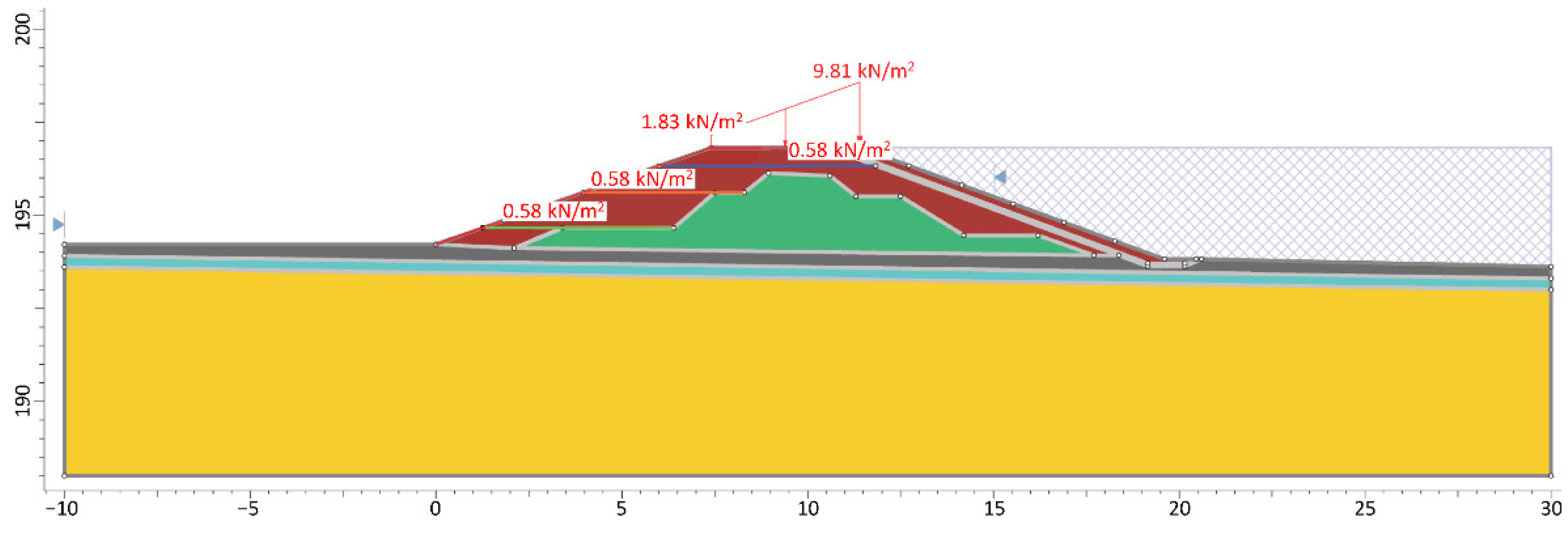
where γw (kN/m3) is the unit weight of water. Equation (11) conservatively overestimates results, since the resulting pressure is a little bit higher than the pressure in area above the steady flow [60]. Shear stresses calculated this way are applied along the crown and landside slope, as shown in Figure 4 for the case study numerical model.
Stability analyses aim to find the critical slip surface by using a population-based stochastic algorithm, Cuckoo Search, which searches for non-circular slip surfaces, together with Monte Carlo optimization to potentially find even more critical surfaces [64]. All the slope stability analyses are deterministic with values of the four random variables previously described varied over appropriate ranges, while probabilistic analyses are conducted after the results of deterministic analyses are obtained. The variation is manually performed for the friction angle, while for the geogrids it is performed with the help of Latin Hypercube simulations. It was initially conducted over a range of ±3σ with steps of 1σ to detect the approximate location of the design point and was then corrected to smaller steps closely spaced around the design point.
3. Case Study
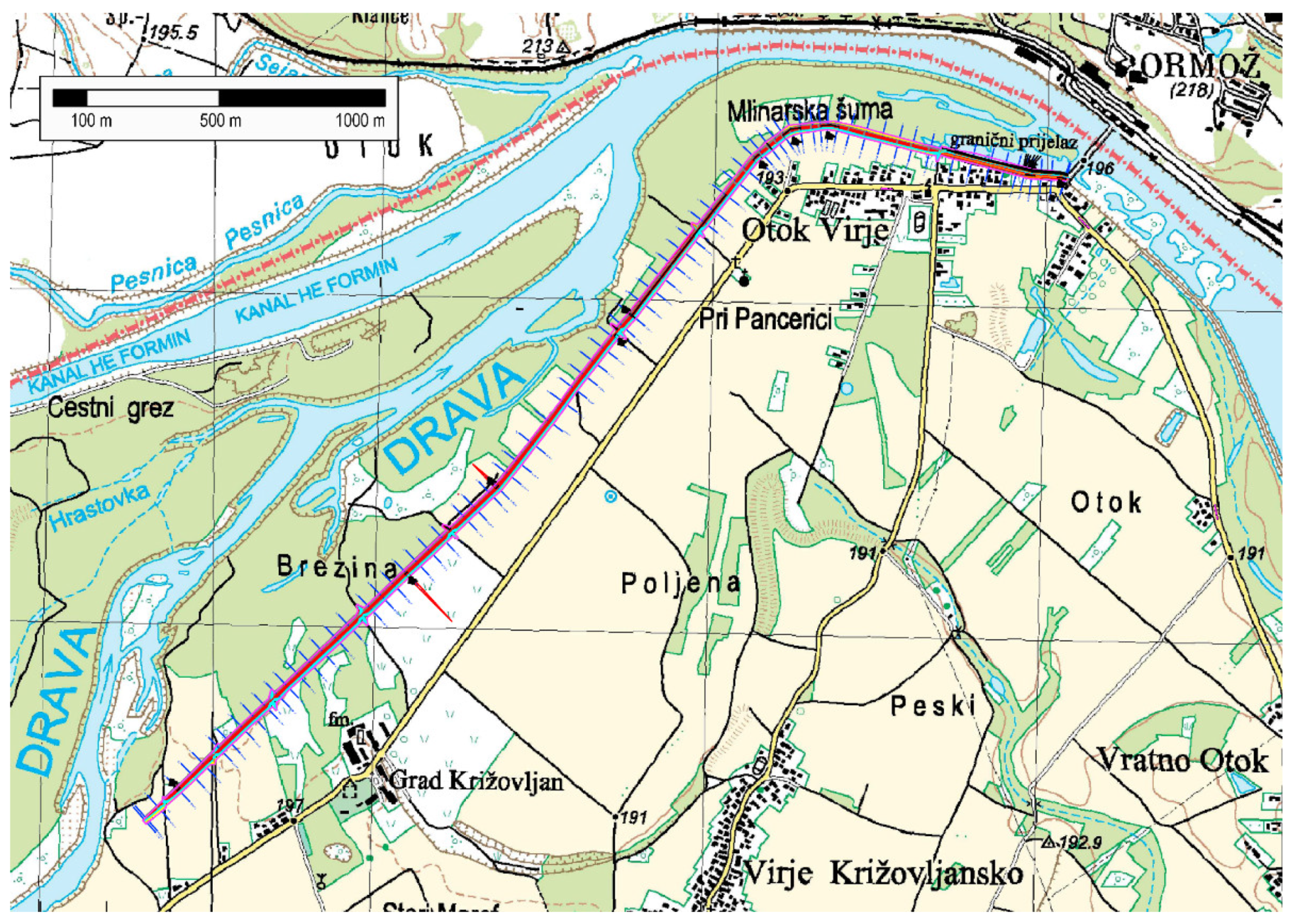
River Drava, with the overall length of 710 km, flows from Italy to eastern Croatia where it merges with Danube, and is historically known for major flood events [65], where prominent events occurred in last several years. For this case study, a reach of a 3.7 km long section of flood protection embankment running from Otok Virje to Brezje on the Drava River in Croatia is analysed. The reach lies on sediments from the Holocene period. They are mostly sediments of the first alluvial terraces of Drava, composed of large amounts of sand and gravel, which at places surpass 100 m in depth. Closer to the surface, layers of silty material can be found.
In 2012, a water level of 1000-year return period was measured in the Drava River, which caused the overflow of the embankment over a length of more than 1 km, and breaching over a length of 50 m, causing huge damages to the surrounding area. Since the original embankment was built in 1968 with the design high water level from 1965 [66], a reconstruction of the existing embankment is required for raising its crown height to new design water levels. The new required height corresponds to the new 100-year return period water level +1 m, which is between a few cm and 1 m above the old crown. Raising the height also implies a widening of the embankment cross section, which can be accomplished in three ways: by keeping the existing embankment on the landward side of the new one (i.e., reconstructing towards the river side), keeping the existing embankment on the river side (i.e., reconstructing towards the landward side), and by coinciding the existing and new axes (i.e., reconstructing on both sides). The selected reach for this case study is defined by the reconstruction direction and subsoil stratigraphy—the reconstruction on both sides is chosen. A situational view of the embankment section on the Drava River is shown in Figure 5.
To prove the stability of the newly reconstructed embankment in all the relevant design situations, calculations are made using deterministic limit equilibrium analyses, and all according to valid norms for geotechnical design, i.e., EN 1997-1:2012 Eurocode 7: Geotechnical design—Part 1: General rules and its respective Croatian national annex for static design situations, EN 1998-1:2011 Eurocode 8: Design of structures for earthquake resistance—Part 1: General rules, seismic actions and rules for buildings and its respective national annex for seismic design. The analyses resulted in the deterministic safety factors shown in Table 1. It can be seen that safety factor values for all design situations are acceptable.
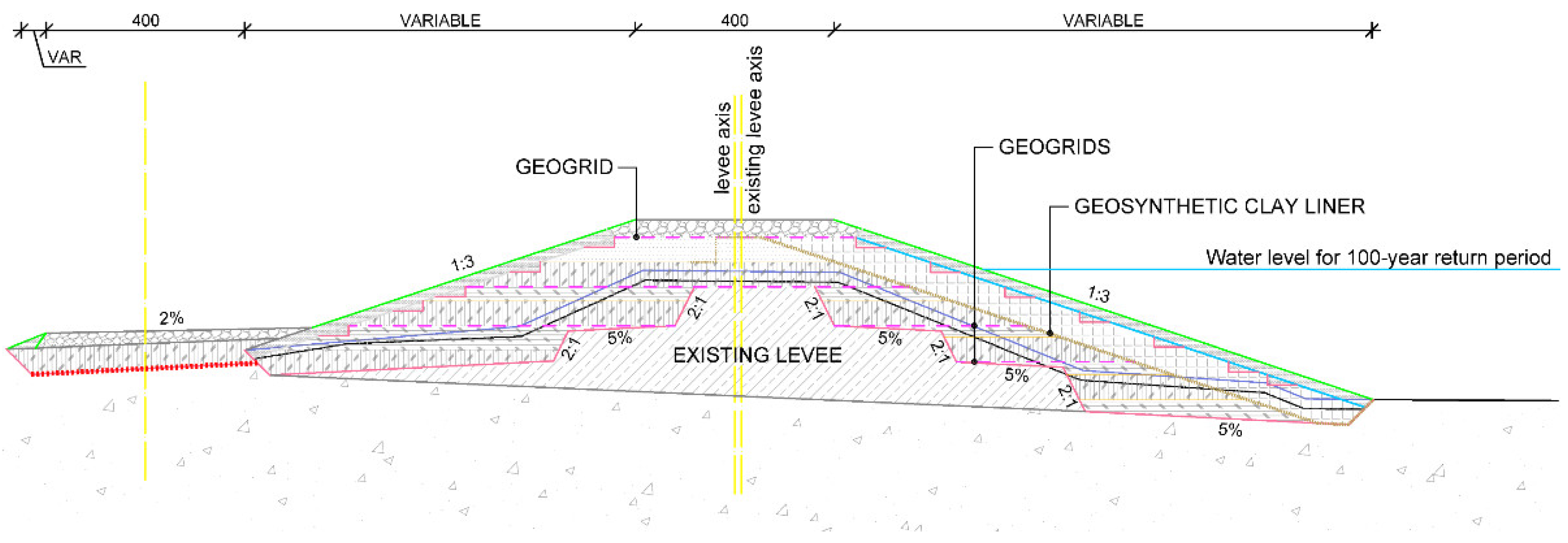
The reconstruction of the levee is made with well graded gravel (GW by USCS classification). Since gravel is highly permeable, GCL membranes are used to make sure the free water surface stays inside the levee body during high water events. Suzuki et al. [67] performed field and laboratory tests with various types of GLC to find their effect on the stability of the embankments. However, since the GCL in this study is located on the riverside of the levee, while the stability of the landside is analysed, their effect is not relevant for this study. Other than that, the body is further strengthened using TENAX TT 045 GS, HDPE uniaxial geogrids. The embankment’s cross section used in calculations is shown in Figure 6. Geogrids are placed on 0.7 and 0.9 m distance from one another to fit the height of the embankment, while the maximum suggested height for reinforced slopes as per [31] is 1 m due to local face stability. This way, local face instabilities are partly mitigated. Instabilities on the landside may also be initiated by surface erosion during overflow. The resistance against such action can be increased by placing a reinforcing layer of standard geosynthetics or other specific products [68] such as biopolymers [69,70] over the slope, but in this case, there is no such additional protection. The same applies for the riverside slope where surface erosion might be caused by the flow of the river and during the rapid decrease of water level in the river (RDD).
Variability of Materials’ Parameters
Deterministic parameters for all soils are carefully chosen from the available laboratory and field data conducted by the authors of this paper. The mean values of geogrid parameters are taken from the manufacturer’s specification sheet. Statistics for the parameters assigned as random variables are chosen from literature. Table 2 shows the design values of deterministic parameters for each material, while Table 3 shows the statistics of the random variables. As all three grids inside the embankment are the same, their statistics are also the same, but each grid is modelled as an independent random variable.
The statistical parameters for the geogrids are determined as follows. The mean value is taken from the manufacturer’s specification sheet where the characteristic value is divided by a series of factors, namely the factor for installation damage (RFID), creep (RFC), and degradation due to chemical and/or biological processes (RFD), to obtain a design tensile strength of 18.5 kN/m. To transform the manufacturer’s proposed long term design strength into a random variable, it is first multiplied with the mean values of bias factors for installation damage (), creep () and durability (), whose statistics are determined from literature [71,72,73,74] to obtain the mean, while the CoVs of different bias factors are together taken as the CoV for tensile strength (Equation (12)). Theoretically, this is valid for uncorrelated log-normal random variables, but with small CoVs it is sufficiently accurate for uncorrelated normal random variables [75]. Since the durability factor is mostly project-specific, it is taken with an arbitrary CoV = 0.1 [72]. Chosen statistics for all factor’s bias values are shown in Table 4. The chosen geogrids are made from HDPE (High Density Polyethylene), which showed the lowest mean and CoV of the bias factors values, and their statistics are found to be independent of soil type [72]. As the random variables of the geogrids are normally distributed [72] and uncorrelated, the simple conversion to standard normal variables as shown in Equation (1) can be employed.
Since partial factors in various design approaches are calibrated using reliability analyses [76], the mean friction angle of the reconstruction material is left at its characteristic value and the variability is applied to it, while all the other deterministic values are factored using partial factors from Eurocode 1997 DA3.
4. Results and Discussion
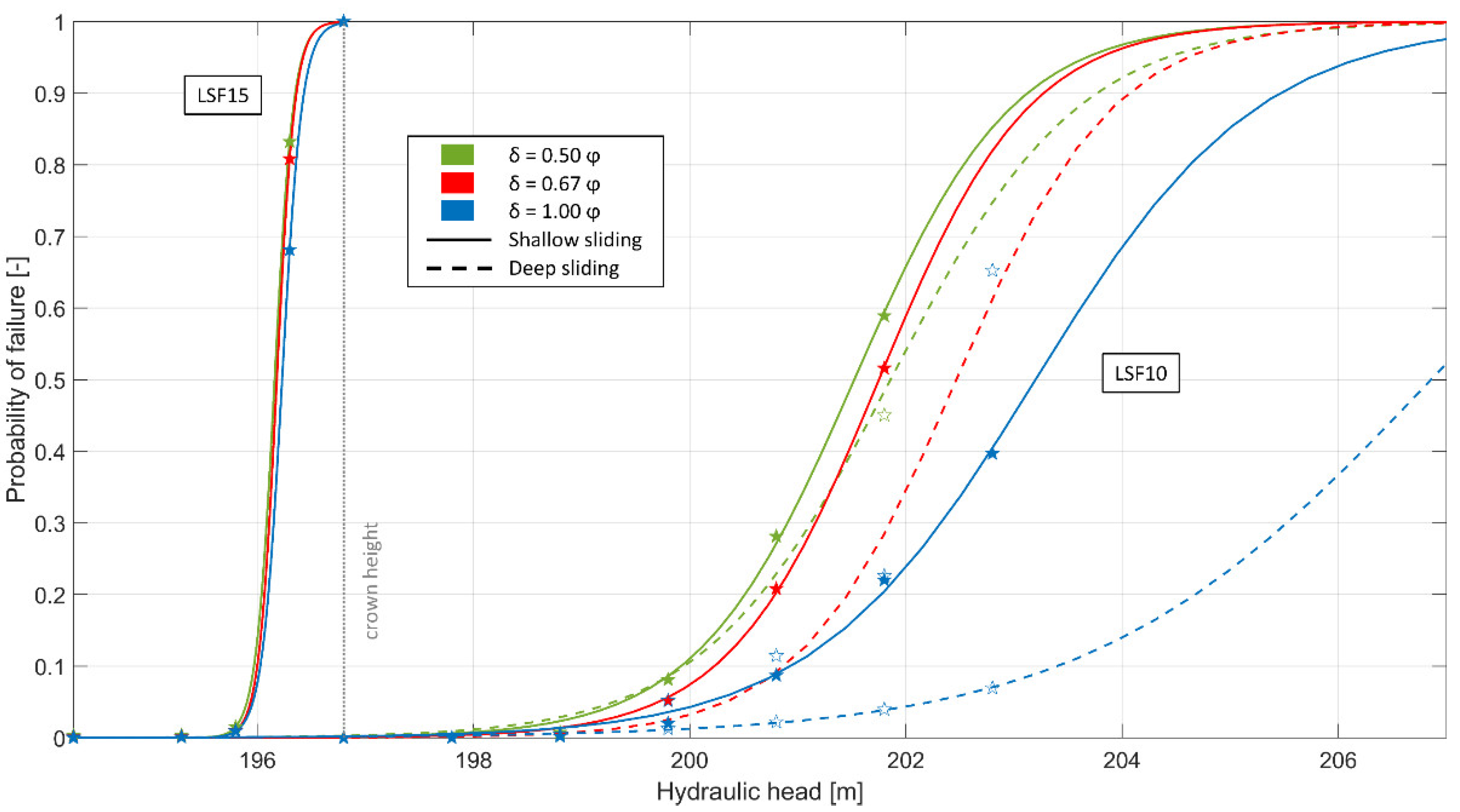
During slope stability calculations at higher water levels, small variations in random variables’ values resulted in shallow and deep sliding surfaces with highly different safety factors, such as those shown in Figure 7. In such cases, the shallow and deep surfaces are separated, and two probabilities of failure are calculated, one pertaining to the shallow sliding and the other to deep sliding. Fragility curves are then constructed for two limit states defined by safety factors 1 and 1.5 (LSF10 and LSF15 respectively), for both types of failures. Figure 8 shows the resulting fragility curves for the two limit states, for varying water levels from the toe to the crown of the levee (located at 196.8 m.a.s.l.), and over to simulate surge overflow. The water level is increased until almost certain failure is ensured. However, Rackwitz [51] noted that FORM works well only for sufficiently large reliability indices, which he defined as β > 1, as otherwise it might not be the best linearization point [77], which in this case corresponds to water level of around 200.5 m.a.s.l. for LSF10, and 196 m.a.s.l. for LSF15. The curves used to fit the points are represented by general sigmoid function with the following equation [78]:
where pf,min and pf,max are minimum and maximum values of the function respectively, the mean hydraulic head, and k is the slope of the curve at the mean value. The curve is fitted to the points using least-squares. By using such a function, a curve can be defined even by not having the whole range of points from zero to one probability of failure. As can be seen from the figures, for the cases where the limit state function is defined by FS = 1.5 (LSF15), the probabilities of failure occur over the whole range, and certain limit-state-behaviour with probability of one is already reached at the crown water level. For the limit state function defined by FS = 1 (LSF10), the maximum calculated probabilities of failures reach from around 65% to as low as 10%, while the rest of the curve is based just on the fitting to those smaller values.
From the diagrams it is seen that with increasing interface friction, the distinction between shallow and deep surfaces starts to show earlier, i.e., at lower water levels, for LSF10. For , the distinction occurs at pf > 0.3, for at pf > 0.05, and for at pf > 0.002. Regardless, this effect never reached water levels as low as the levee crown for this case. For the LSF15, the distinction occurs at lower water levels rather than higher and is not so large, which is the reason why it is not noticeable on the normal scale. Also, the interface friction in this regard does not have any noticeable effect in this case. At water levels where there is no distinction between deep and shallow surfaces, this happens because of two reasons. One is that all the failures occurred as either deep or shallow failures, and the other is that there is little distinction between safety factors of deep and shallow surfaces. The first reason indicates that the curves are constructed for the stability of the slope regardless of the failure mode, as long as all the surfaces followed the same mode. Only when different modes appear, the curves become separated.
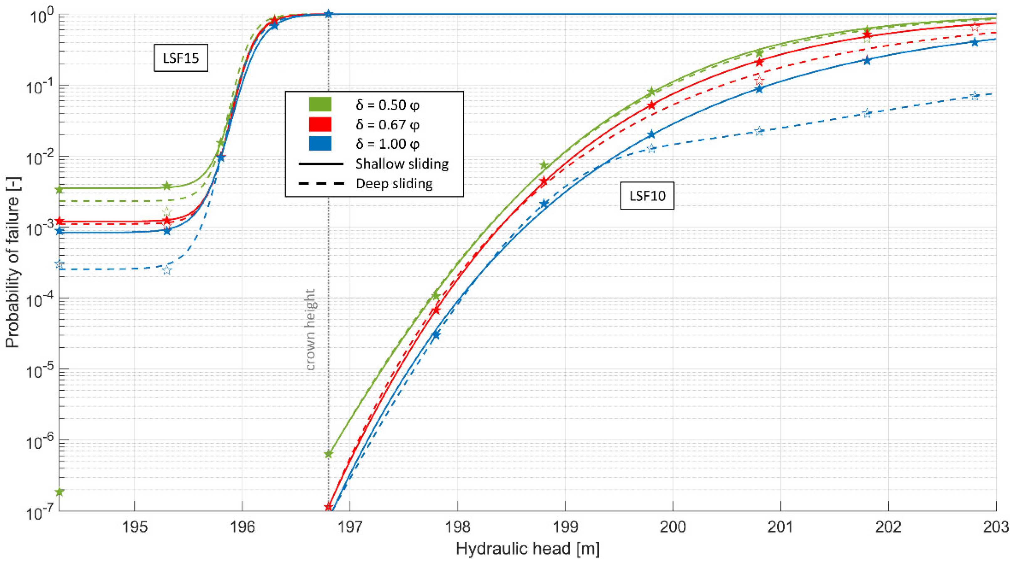
Even though the diagrams for both limit states seem to merge at lower water levels, obviously this is not the case because the diagrams refer to different limit states which cannot be achieved with the same strength parameters for a specific water level. Thus, Figure 9 shows the diagram in a logarithmic scale to see the difference at lower water levels. The LSF15 points can still be approximated as relatively good by the same sigmoid function. For LSF15 the probability of failure starts to noticeably increase only after the water level reaches circa 60% of the levee height. On the other hand, the LSF10 points have a worse fit which is caused by the fact that the pf stays almost the same for water levels between 0 and the levee crown, and start to substantially change only for the surge overflow. Thus, to fit the LSF10 points, the first point referring to a no-water situation is ignored. The reason for the constant probability of failure is that the parameters needed to achieve the defined limit state are such that they produce small slip surfaces on which water has no effect in this case. This means that regardless of the water level up to the crown, the pf of the levee stays the same. It can be noted from the figures that deeper failure surfaces are generally less likely to occur during failure than shallower surfaces. This is certainly conditioned by the fact that the levee body through which the deeper surfaces pass has been modelled as a deterministic material. An interesting thing to note for the minimum friction LSF15 case is that the points which refer to deep surfaces show a slight decrease of pf with the increase of the water level at the beginning of the curve. This means that for the lower water level there is a higher probability that the levee will fail overall, than there is for the higher water level that the levee will fail through deep sliding. The reason for such behaviour is because, for the smaller water level, no deep surfaces are found. For other interface friction angles, these two values are quite similar.
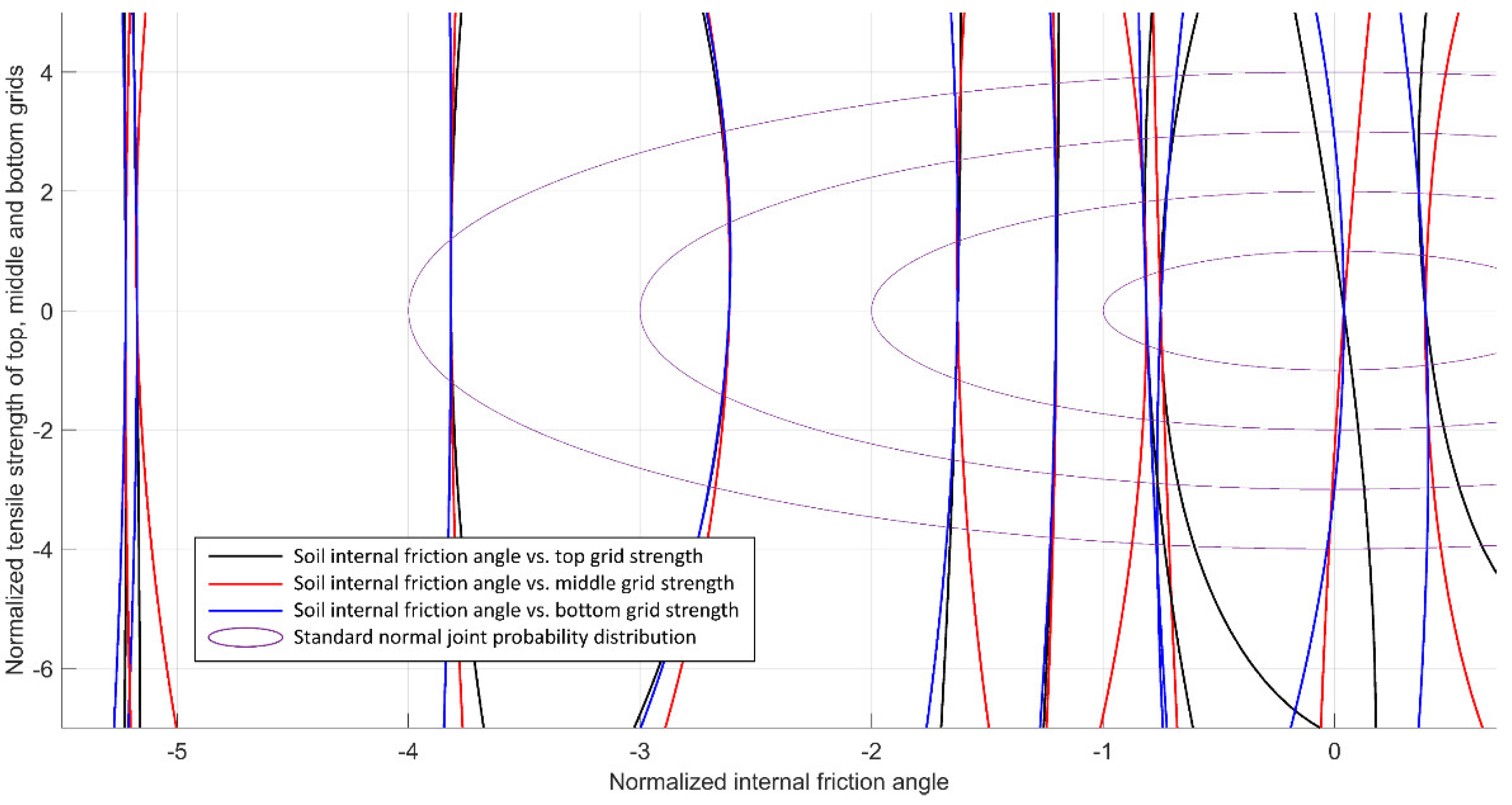
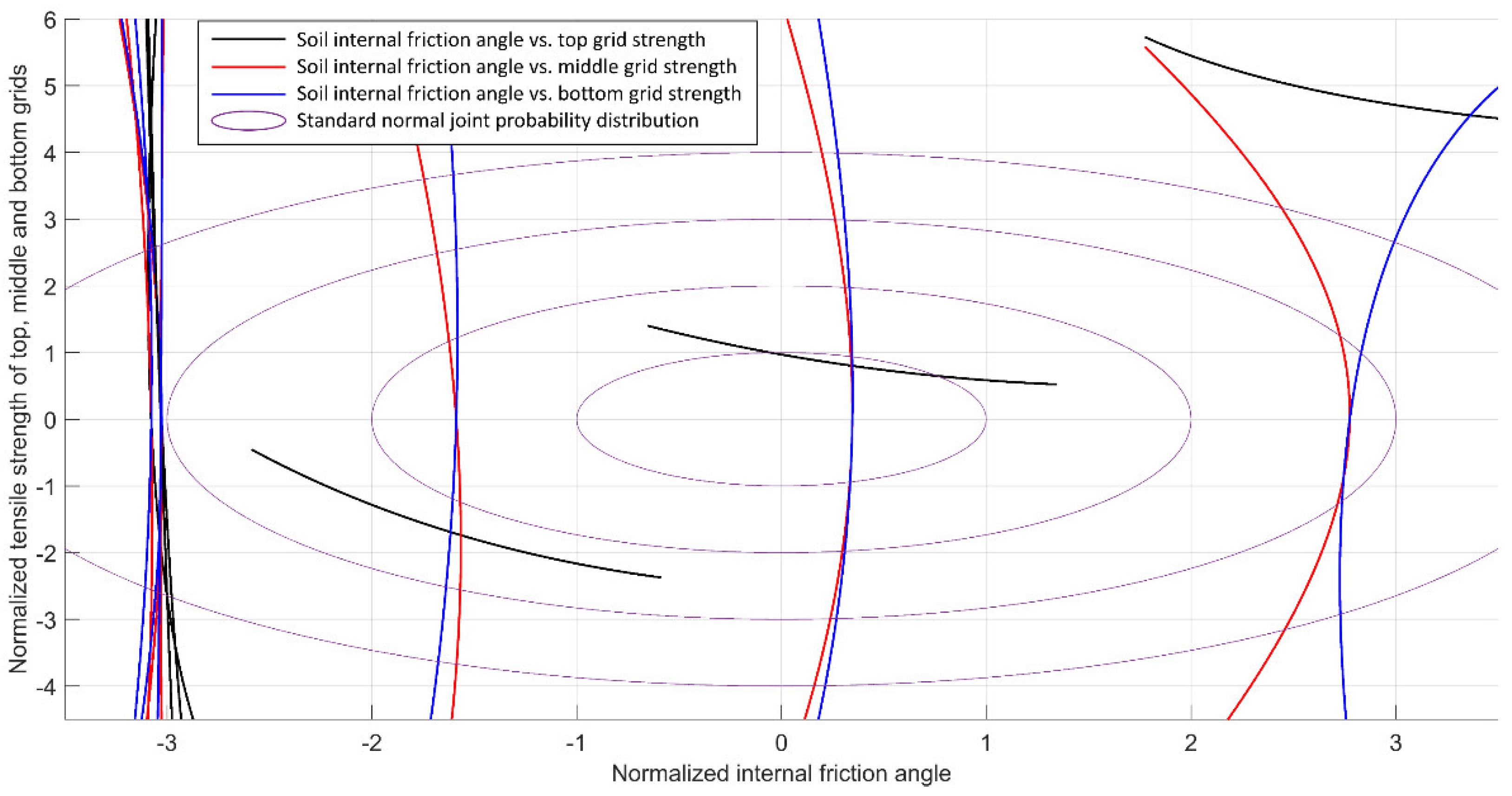
While interpreting the results of computed conditional probabilities of failure, it must be kept in mind that they are calculated based on only one point closest to the origin, defined by the reliability index. This implies the linearization of the limit state function for integration below the standard normal joint distribution, which can lead to an overestimation or underestimation of the real probability, depending on the true shape of the limit state function [52]. To investigate their shapes, 2D representations of the limit state functions for mean interface friction, and for LSF10 and LSF15, are shown in Figure 10, where the black lines represent LSFs for soil internal friction and top grid strength as random variables, red lines LSFs for soil internal friction and middle grid strength as random variables, and blue lines LSFs for soil internal friction and bottom grid strength as random variables. The rightmost curves correspond to higher water levels, decreasing towards the leftmost curves. The circles in Figure 10 represent the standard normal joint distribution, i.e., each circle corresponds to one standard deviation. From the figures it can be seen that LSFs are slightly curved in either direction, without any notable trend, thus giving mixed results in terms of conservativeness. However, the effect of linearization is not expected to be high in most cases due to the curvatures being relatively mild. Similar shapes are noted for all interface friction angle values and are not shown here.
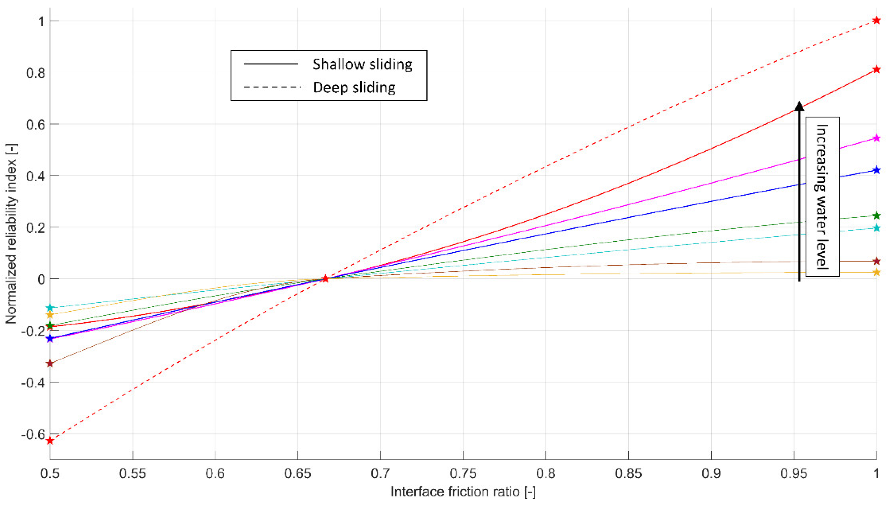
To better investigate the effect of increasing reliability with increase of interface friction ratio, defined as δ/φ, graphs are plotted in Figure 11 showing these trends for LSF10 with the normalized reliability index on the vertical axis. The normalized reliability index is simply the reliability index for the mean interface friction ratio for each respective water level subtracted from the reliability indices at other friction ratios (βn = β − β0.67). This way all the curves are translated over the vertical axis for better comparison. From Figure 11 two characteristics are noticed, one being that the trend is approximately linear, changing from a power law for the lower water levels (i.e., higher β, lower pf) to a positive parabola for the higher water levels (i.e., lower β, higher pf). The second relates to the increase of steepness of the curve from lower to higher water levels, which is more pronounced on the higher friction ratio than on the lower. Also, the same increasing effect is seen for deeper versus shallow surfaces for the same water level (the two highest curves). For the LSF15 case (not shown on figures), even though some differences apparently exist between pfs for different friction ratios, there are no visible trends, except for the deep sliding curve being steeper than the corresponding shallow sliding curves.
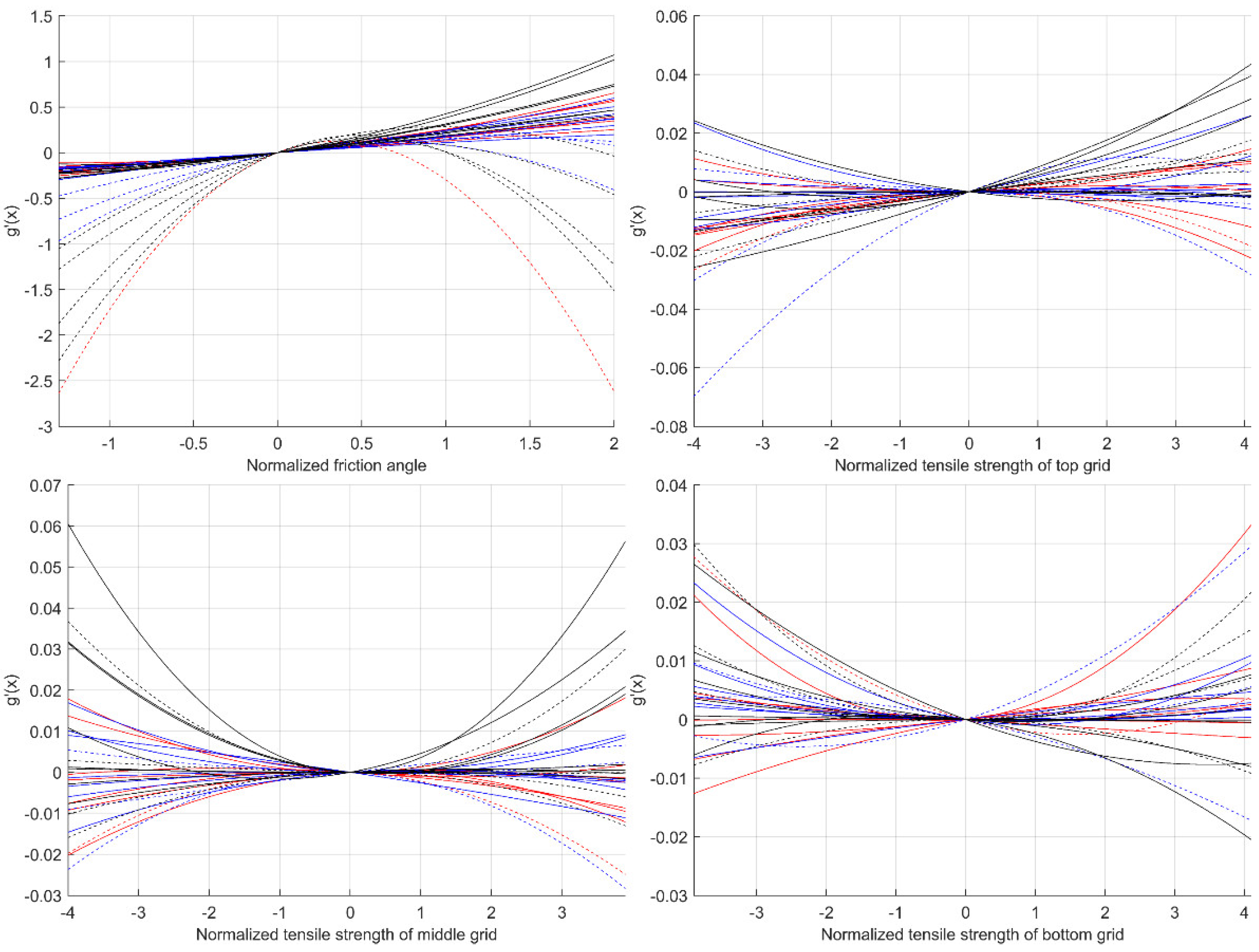
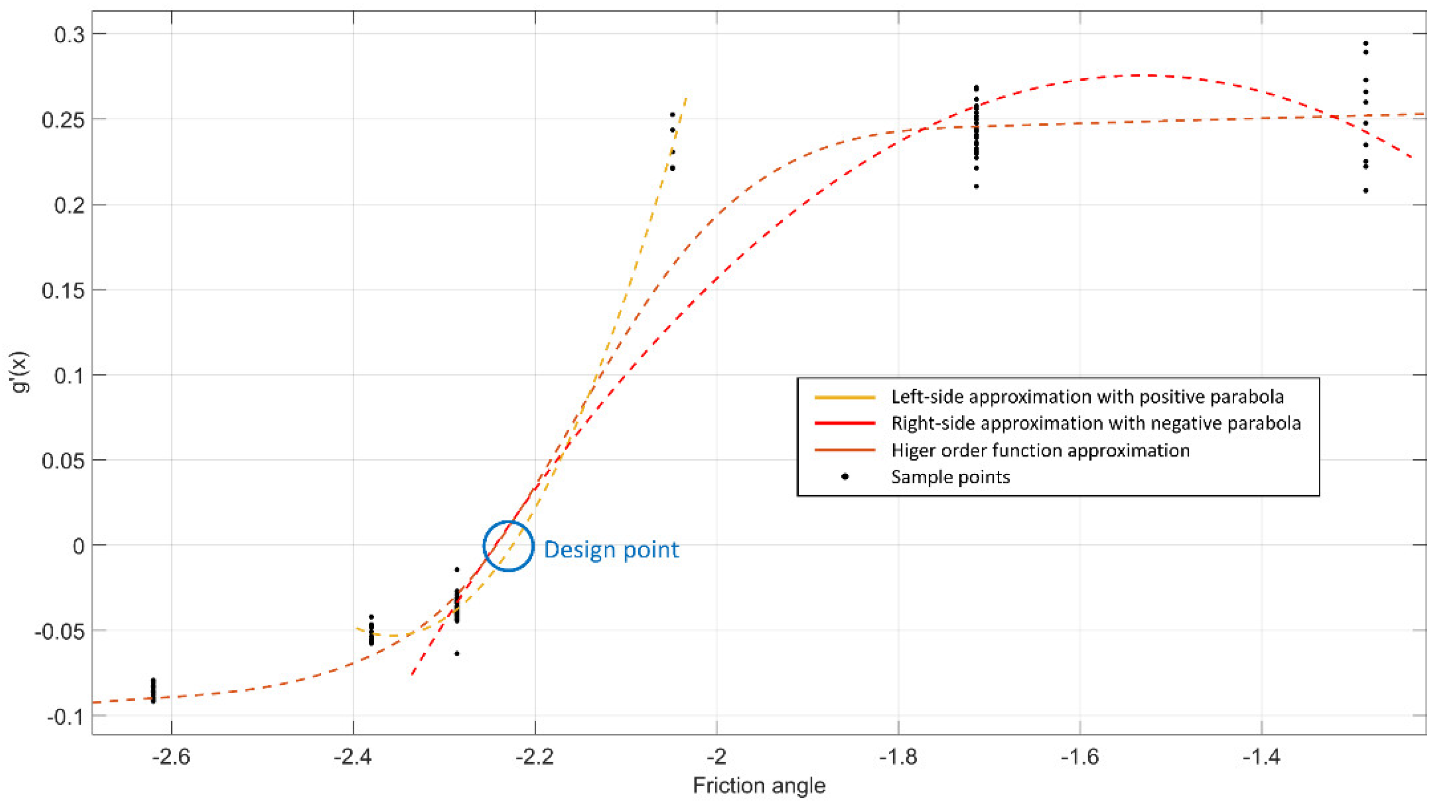
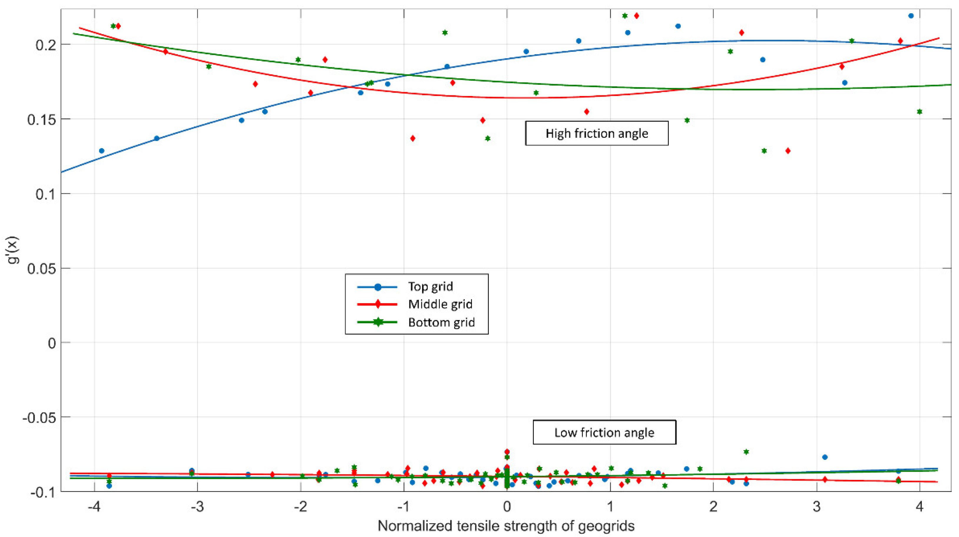
To analyse the sensitivity of the slope stability to each of the defined random variables, 2D sections of the response surfaces through the design point are plotted on Figure 12. For each graph, one variable of interest is varied in the vicinity of the design point, while the other random variables are held at their respective design point values. The horizontal axes on the graphs are normalized such that the design point value is at zero and show the number of standard deviations away from the point. In other words, the curves are shifted from values obtained through Equation (1) to align all the design points at zero. This helps comparing the trends of the response surface at various water levels. From the response surfaces, it is found that two main trends exist, namely parabolic (positive or negative) and linear. This is of course constrained by the function used to approximate the response surface (Equation (4)), which is a quadratic polynomial. It is intuitive that the increase of any strength or resistance parameter’s value causes the stability of a slope to increase by increasing the safety factor. However, some curves shown in Figure 12 seem to contradict this statement as they are parabolas which have maxima and minima at, or close to, the design point. This is just an apparent problem caused only by the chosen approximation function and does not show any inconsistencies considering the friction angle because all the maxima are found on the right side of the design point, while all the minima are found on the left side, and the curves are fitted to the data by their increasing parts. This mostly occurred when smaller friction angles did not have a distinction between deep and shallow sliding, but higher friction angles did have it. In those cases, a sudden increase in safety factor occurs and a parabolic response surface cannot be generated with the whole range of data for deep sliding. This means that to achieve a good fit of the data to a parabola, one needs to discard all but the closest sample points on either side of the design point, while only keeping all the points on the opposite side. An example of such situation is shown in Figure 13. It is obvious that a higher order function should be used to approximate such data. It could be argued that if only a narrow range of data around the design point is used, then there would be no need to approximate the data using higher order function. While this may be true in some cases, in other cases the range which would be needed to avoid higher order functions is relatively narrow, and would complicate the analysis to find values only inside that narrow range.
For the geogrids’ tensile strengths, the trends are generally constant, which means they do not affect the safety factor. However, there are multiple increasing curves, and others which actually do show a decrease of the safety factor with a strength increase. Regarding the latter, it should be noted that the range of safety factors on Figure 12 for the grids is from 0.95 to 1.05, and thus such trends cannot be deemed as true trends. They can instead be attributed to data scatter in both deep and shallow surfaces, as well as to the shape limitations of the selected approximation function. This data scatter occurs mostly for the bottom and middle grid layers, and only at the higher end of friction angles. In the same region of friction angles, the top grid’s strength start showing a linear to parabolic trend, as shown in Figure 14. This kind of data, however, also did not cause any inconsistencies with results, as the design point tensile strengths are practically at the mean values for most cases (Figure 15).
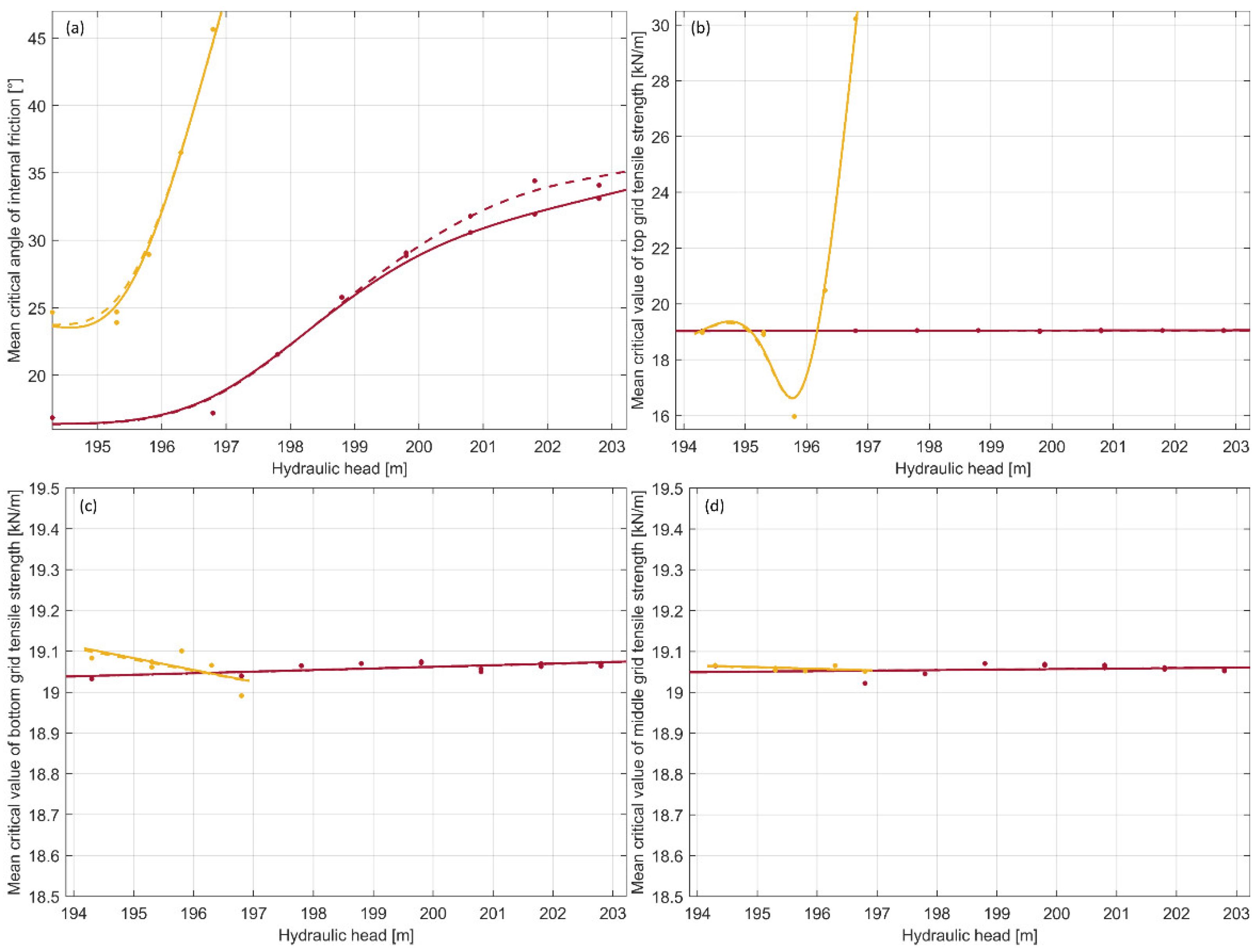
With each increment in water level there is change in probability of failure/reliability index, which is caused by the different critical values of random variables needed to reach a specific LSF at that specific water level. Even though the critical values differ when the same water level is evaluated with different interface friction ratios, because the difference is not large, Figure 15 shows the mean critical value of each random variable. Figure 15 is a representation of Equation (5), where the total reliability index can also be calculated for each water level by knowing the corresponding critical values of each random variable. Even though Figure 15b shows a decrease in critical tensile strength for the LSF15 at hydraulic head near 196 m.a.s.l. compared to lower heads, the reliability index still decreases (Figure 8 and Figure 9) due to an increase in critical friction angle. On the other hand, the critical value for the LSF10 shows practically no change with the increase of water level. This is also true for both LSFs for the middle and bottom grids.
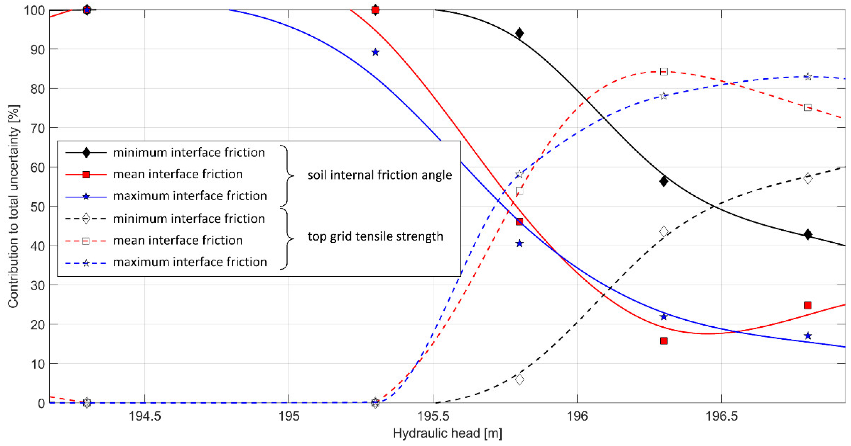
To investigate the relative contribution of the uncertainty of each random variable to the total uncertainty, the direction cosines (or sensitivity factors) are calculated as the ratio of each random variable’s critical value to the reliability index. The squared sensitivity factors give us the values of interest [79]. For all interface friction angles (low, mean, high) for LSF10, the contribution of the internal friction angle is >99.84%, with a mean value of 99.97%. The small remainder (<0.15% of total uncertainty) belongs to all three layers of geogrids, with almost 3/4 of that belonging to the top grid, and the rest somewhat evenly distributed between the middle and bottom grids. For LSF15, the relative contribution of the internal friction angle decreases with the increase of water level, from almost 100% to 17%, while the rest is attributed to the top grid, as shown in Figure 16. The middle and bottom grid’s contribution stayed close to zero at all times.
5. Conclusions
It should be noted that conclusions drawn from this study are only valid for systems similar to the analyzed levee, where local face stability in ensured between geogrid layers, and where there is no anchorage on the front face, which would increase stability even more at the cost of additional material for the anchorage. From the presented results, a few conclusions can be drawn:
- Close to the ULS, at higher water levels (in this case pf > 0.002), small variations in random variables cause deep and shallow sliding surfaces with highly different safety factors and pfs. With the increase of interface friction angle, the water level at which this distinction becomes visible decreases. Farther from the ULS, this effect occurs at low water levels rather than higher, and the interface friction doesn’t have any noticeable effect on the occurrence. Shallow sliding is shown to be more likely to occur for both limit states.
- Linearization of the performance function required for calculation of the probability of failure with the FORM does not influence the results greatly as the curvatures of the limit state functions are generally not large.
- The increase of reliability with increase in interface friction ratio is approximately linear in proximity of the ultimate limit state, with higher steepness for higher water levels. Also, deep surfaces seem to have a steeper curve than shallow surfaces. This is not true farther away from the ULS.
- Constant, linear, and parabolic trends, and those of higher order, are found for the performance function dependency to the reconstruction material friction angle and to the geogrid layers. The order of the function tends to increase with water level, i.e., with probability of failure. The higher order trends occur mostly for deep sliding when a sudden increase of safety factor occurs as a result of small increase in friction angle of the levee body. For this reason, quadratic functions should be used with care, and perhaps a function with an inflection point (e.g., cubic function) should be employed in some cases.
- The internal friction angle contributes almost completely to the total uncertainty when close to the ULS (the contribution of the grids is negligible). However, it seems that geogrids placed near the top contribute the most out of all the geogrids.The contribution of the internal friction angle seems to diminish going farther away from the ULS (e.g., LSF15), and it transfers to the grid placed near the top, while the other grids’ contribution remains negligible.This importance of the top grid, however, needs to be considered carefully, because in this study the top grid is the only one that goes from one slope of the levee to the other, while the middle and bottom grids are only placed on one side. The relative contribution might be different in case all grids are the same length.
- The reason for the grids’ extremely low contribution to the total uncertainty lies with the small variability of their tensile strengths. But as seen in the LSF15 case, as the required critical tensile strength reaches the actual tensile strength, their variability has more effect on the stability, which indicates a way of determining the required strength for each grid layer. Moreover, since the increase of both the soil friction angle and the soil-grid interface friction individually tend to generate deeper surfaces, it is implied that a balance between these parameters can be found. Both procedures would lead to a balanced reinforced slope design with regard to geogrid rupture strength and geogrid pull out.
At this time, deterministic analyses are still the dominant type of analyses when it comes to designing levees for flood protection in terms of slope stability. These calculations require safety factors >1 to be acceptable by definition of the safety factor. However, it is rarely deemed acceptable to reach safety factors around one, and higher values are often targeted. This study deals with slope stability of a geogrid reinforce levee in a probabilistic manner, and shows trends in the response of the levee and behaviour of the reinforcement components for two target safety factors of one and 1.5. Even though some trends are not as clear as others, and/or they are not quantitatively defined, and for which further investigations are needed, the identified trends might still serve as guidelines for design and can be loosely interpolated (where applicable) to increase understanding of the system behaviour for a targeted safety level.
Author Contributions
Conceptualization, N.R. and M.S.K.; Formal analysis, N.R.; Investigation, N.R., M.B., M.S.K. and L.L.; Methodology, N.R. and M.S.K.; Software, N.R.; Supervision, M.S.K.; Validation, N.R., M.B. and M.S.K.; Visualization, N.R.; Writing—original draft, N.R. and M.B.; Writing—review and editing, M.S.K. and L.L. All authors have read and agreed to the published version of the manuscript.
Funding
This research was funded by European Union Civil Protection Mechanism, under UCPM-2019-PP-AG call, Grant Agreement Number 874421, oVERFLOw project (Vulnerability assessment of embankments and bridges exposed to flooding hazard).
Conflicts of Interest
The authors declare no conflict of interest. The funders had no role in the design of the study; in the collection, analyses, or interpretation of data; in the writing of the manuscript, or in the decision to publish the results.
References
- Wang, X.; Wang, L.; Zhang, T. Geometry-Based Assessment of Levee Stability and Overtopping Using Airborne LiDAR Altimetry: A Case Study in the Pearl River Delta, Southern China. Water 2020, 12, 403. [Google Scholar] [CrossRef] [Green Version]
- Elias, V.; Christopher, B.R.; Berg, R.R. Mechanically Stabilized Earth Walls and Reinforced Soil Slopes Design and Construction Guidelines; National Highway Institute, Federal Highway Administration, U.S. Department of Transportation: Washington, DC, USA, 2001.
- Avesani Neto, J.O.; Bueno, B.S.; Futai, M.M. A Bearing Capacity Calculation Method for Soil Reinforced with a Geocell. Geosynth. Int. 2013, 20, 129–142. [Google Scholar] [CrossRef]
- Kolay, P.K.; Kumar, S.; Tiwari, D. Improvement of Bearing Capacity of Shallow Foundation on Geogrid Reinforced Silty Clay and Sand. Available online: https://www.hindawi.com/journals/jcen/2013/293809/ (accessed on 16 November 2020).
- Wang, J.-Q.; Zhang, L.-L.; Xue, J.-F.; Tang, Y. Load-Settlement Response of Shallow Square Footings on Geogrid-Reinforced Sand under Cyclic Loading. Geotext. Geomembr. 2018, 46, 586–596. [Google Scholar] [CrossRef]
- Barani, O.R.; Bahrami, M.; Sadrnejad, S.A. A New Finite Element for Back Analysis of a Geogrid Reinforced Soil Retaining Wall Failure. Int. J. Civ. Eng. 2018, 16, 435–441. [Google Scholar] [CrossRef]
- Wang, J.-Q.; Xu, L.-J.; Xue, J.-F.; Tang, Y. Laboratory Study on Geogrid Reinforced Soil Wall with Modular Facing under Cyclic Strip Loading. Arab. J. Geosci. 2020, 13, 398. [Google Scholar] [CrossRef]
- Wang, H.; Yang, G.; Wang, Z.; Liu, W. Static Structural Behavior of Geogrid Reinforced Soil Retaining Walls with a Deformation Buffer Zone. Geotext. Geomembr. 2020, 48, 374–379. [Google Scholar] [CrossRef]
- Abu-Farsakh, M.Y.; Akond, I.; Chen, Q. Evaluating the Performance of Geosynthetic-Reinforced Unpaved Roads Using Plate Load Tests. Int. J. Pavement Eng. 2016, 17, 901–912. [Google Scholar] [CrossRef]
- Cuelho, E.V.; Perkins, S.W. Geosynthetic Subgrade Stabilization—Field Testing and Design Method Calibration. Transp. Geotech. 2017, 10, 22–34. [Google Scholar] [CrossRef] [Green Version]
- Varuso, R.J.; Grieshaber, J.B.; Nataraj, M.S. Geosynthetic Reinforced Levee Test Section on Soft Normally Consolidated Clays. Geotext. Geomembr. 2005, 23, 362–383. [Google Scholar] [CrossRef]
- Ferreira, F.B.; Topa Gomes, A.; Vieira, C.S.; Lopes, M.L. Reliability Analysis of Geosynthetic-Reinforced Steep Slopes. Geosynth. Int. 2016, 23, 301–315. [Google Scholar] [CrossRef]
- Hird, C.C.; Kwok, C.M. Finite Element Studies of Interface Behaviour in Reinforced Embankments of Soft Ground. Comput. Geotech. 1989, 8, 111–131. [Google Scholar] [CrossRef]
- Rowe, R.K.; Li, A.L. Reinforced Embankments over Soft Foundations under Undrained and Partially Drained Conditions. Geotext. Geomembr. 1999, 17, 129–146. [Google Scholar] [CrossRef]
- Rowe, R.K.; Gnanendran, C.T.; Landva, A.O.; Valsangkar, A.J. Calculated and Observed Behaviour of a Reinforced Embankment over Soft Compressible Soil. Can. Geotech. J. 1996. [Google Scholar] [CrossRef]
- Balakrishnan, S.; Viswanadham, B.V.S. Evaluation of Tensile Load-Strain Characteristics of Geogrids through in-Soil Tensile Tests. Geotext. Geomembr. 2017, 45, 35–44. [Google Scholar] [CrossRef]
- Zheng, G.; Yu, X.; Zhou, H.; Wang, S.; Zhao, J.; He, X.; Yang, X. Stability Analysis of Stone Column-Supported and Geosynthetic-Reinforced Embankments on Soft Ground. Geotext. Geomembr. 2020, 48, 349–356. [Google Scholar] [CrossRef]
- Rowe, R.K.; Soderman, K.L. An Approximate Method for Estimating the Stability of Geotextile-Reinforced Embankments. Can. Geotech. J. 1985. [Google Scholar] [CrossRef]
- Deng, M. Reliability-Based Optimization Design of Geosynthetic Reinforced Embankment Slopes. Ph.D. Thesis, Missouri S&T, Rolla, MO, USA, 2015. [Google Scholar]
- Sharma, P.; Mouli, B.; Jakka, R.S.; Sawant, V.A. Economical Design of Reinforced Slope Using Geosynthetics. Geotech. Geol. Eng. 2020, 38, 1631–1637. [Google Scholar] [CrossRef]
- Rowe, R.K.; Li, A.L. Geosynthetic-Reinforced Embankments over Soft Foundations. Geosynth. Int. 2005, 12, 50–85. [Google Scholar] [CrossRef]
- Derghoum, R.; Meksaouine, M. Coupled Finite Element Modelling of Geosynthetic Reinforced Embankment Slope on Soft Soils Considering Small and Large Displacement Analyses. Arab. J. Sci. Eng. 2019, 44, 4555–4573. [Google Scholar] [CrossRef]
- Avesani Neto, J.O.; Bueno, B.S.; Futai, M.M. Evaluation of a Calculation Method for Embankments Reinforced with Geocells over Soft Soils Using Finite-Element Analysis. Geosynth. Int. 2015, 22, 439–451. [Google Scholar] [CrossRef]
- Mehrjardi, G.T.; Ghanbari, A.; Mehdizadeh, H. Experimental Study on the Behaviour of Geogrid-Reinforced Slopes with Respect to Aggregate Size. Geotext. Geomembr. 2016, 44, 862–871. [Google Scholar] [CrossRef]
- Tandjiria, V.; Low, B.K.; Teh, C.I. Effect of Reinforcement Force Distribution on Stability of Embankments. Geotext. Geomembr. 2002, 20, 423–443. [Google Scholar] [CrossRef]
- Mulabdić, M.; Kaluđer, J.; Minažek, K.; Matijević, J. Priručnik za Primjenu Geosintetika u Nasipima za Obranu od Poplava (Manual for Application of Geosynthetics in Flood Protection Embankments); Faculty of Civil Engineering Osijek: Osijek, Croatia, 2016. [Google Scholar]
- Moraci, N.; Cardile, G.; Gioffrè, D.; Mandaglio, M.C.; Calvarano, L.S.; Carbone, L. Soil Geosynthetic Interaction: Design Parameters from Experimental and Theoretical Analysis. Transp. Infrastruct. Geotech. 2014, 1, 165–227. [Google Scholar] [CrossRef] [Green Version]
- Skejic, A.; Medic, S.; Ivšić, T. Numerical Investigations of Interaction between Geogrid/Wire Fabric Reinforcement and Cohesionless Fill in Pull-out Test. Gradevinar 2020, 72, 237–252. [Google Scholar] [CrossRef]
- Strata Systems, Inc. Reinforced Soil Slopes and Embankments; Strata Systems, Inc.: Cumming, GA, USA, 2010. [Google Scholar]
- Yamanouchi, T.; Fukuda, N. Design and Observation of Steep Reinforced Embankments. In Proceedings of the Third International Conference on Case Histories in Geotechnical Engineering, St. Louis, MO, USA, 1–6 June 1993. [Google Scholar]
- GEO. Guide to Reinforced Fill Structure and Slope Design; Geotechnical Engineering Office, Civil Engineering and Development Department, HKSAR Government: Hong Kong, China, 2017; p. 218.
- Wolff, T.F. Reliability of levee systems. In Reliability-Based Design in Geotechnical Engineering; Phoon, K.-K., Ed.; Taylor & Francis: Abingdon, UK, 2008; pp. 448–496. [Google Scholar]
- Kirca, V.S.O.; Kilci, R.E. Mechanism of Steady and Unsteady Piping in Coastal and Hydraulic Structures with a Sloped Face. Water 2018, 10, 1757. [Google Scholar] [CrossRef] [Green Version]
- Bujakowski, F.; Falkowski, T. Hydrogeological Analysis Supported by Remote Sensing Methods as a Tool for Assessing the Safety of Embankments (Case Study from Vistula River Valley, Poland). Water 2019, 11, 266. [Google Scholar] [CrossRef] [Green Version]
- Martinović, K.; Reale, C.; Gavin, K. Fragility Curves for Rainfall-Induced Shallow Landslides on Transport Networks. Can. Geotech. J. 2017, 55, 852–861. [Google Scholar] [CrossRef] [Green Version]
- Li, Y.; Qian, C.; Fu, Z.; Li, Z. On Two Approaches to Slope Stability Reliability Assessments Using the Random Finite Element Method. Appl. Sci. 2019, 9, 4421. [Google Scholar] [CrossRef] [Green Version]
- MacKillop, K.; Fenton, G.; Mosher, D.; Latour, V.; Mitchelmore, P. Assessing Submarine Slope Stability through Deterministic and Probabilistic Approaches: A Case Study on the West-Central Scotia Slope. Geosciences 2019, 9, 18. [Google Scholar] [CrossRef] [Green Version]
- Far, M.S.; Huang, H. A Hybrid Monte Carlo-Simulated Annealing Approach for Reliability Analysis of Slope Stability Considering the Uncertainty in Water Table Level. Procedia Struct. Integr. 2019, 22, 345–352. [Google Scholar] [CrossRef]
- Hu, H.; Huang, Y.; Chen, Z. Seismic Fragility Functions for Slope Stability Analysis with Multiple Vulnerability States. Environ. Earth Sci. 2019, 78, 690. [Google Scholar] [CrossRef]
- Pan, Q.; Qu, X.; Wang, X. Probabilistic Seismic Stability of Three-Dimensional Slopes by Pseudo-Dynamic Approach. J. Cent. South Univ. 2019, 26, 1687–1695. [Google Scholar] [CrossRef]
- Wang, L.; Wu, C.; Gu, X.; Liu, H.; Mei, G.; Zhang, W. Probabilistic Stability Analysis of Earth Dam Slope under Transient Seepage Using Multivariate Adaptive Regression Splines. Bull. Eng. Geol. Environ. 2020, 79, 2763–2775. [Google Scholar] [CrossRef]
- Zhang, S.; Li, Y.; Li, J.; Liu, L. Reliability Analysis of Layered Soil Slopes Considering Different Spatial Autocorrelation Structures. Appl. Sci. 2020, 10, 4029. [Google Scholar] [CrossRef]
- Rossi, N.; Bačić, M.; Kovačević, M.S.; Librić, L. Development of Fragility Curves for Piping and Slope Stability of River Levees. Water 2021, 13, 738. [Google Scholar] [CrossRef]
- Kennedy, R.P.; Cornell, C.A.; Campbell, R.D.; Kaplan, S.; Perla, H.F. Probabilistic Seismic Safety Study of an Existing Nuclear Power Plant. Nucl. Eng. Des. 1980, 59, 315–338. [Google Scholar] [CrossRef]
- DePoto, W.; Gindi, I. Hydrology Manual; Los Angeles County Department of Public Works: Los Angeles, CA, USA, 1991.
- DePoto, W.; Gindi, I. Hydrology Manual; Los Angeles County Department of Public Works: Los Angeles, CA, USA, 1993.
- Jasim, F.H.; Vahedifard, F. Fragility Curves of Earthen Levees under Extreme Precipitation. In Proceedings of the Geotechnical Frontiers 2017 GSP 278, Orlando, FL, USA, 12–15 March 2017; American Society of Civil Engineers: Orlando, FL, USA, 2017; pp. 353–362. [Google Scholar]
- Hasofer, A.M.; Lind, M.C. An Exact and Invariant First Order Reliability Format. J. Eng. Mech. 1974, 100, 111–121. [Google Scholar]
- Singh Arora, J. Additional Topics on Optimum Design. In Introduction to Optimum Design; Academic Press: Cambridge, MA, USA, 2017; pp. 795–849. ISBN 978-0-12-800806-5. [Google Scholar]
- Phoon, K.-K. Numerical recipes for reliability analysis—A primer. In Reliability-Based Design in Geotechnical Engineering; Phoon, K.-K., Ed.; Taylor & Francis: Abingdon, UK, 2008; pp. 1–75. [Google Scholar]
- Rackwitz, R. Reliability Analysis—A Review and Some Perspectives. Struct. Saf. 2001, 23, 365–395. [Google Scholar] [CrossRef]
- Baecher, G.B.; Christian, J.T. The Hasofer-Lind Approach (FORM). In Reliability and Statistics in Geotechnical Engineering; Wiley: Chichester, UK, 2003; pp. 377–397. [Google Scholar]
- Sia, A.H.I.; Dixon, N. Distribution and Variability of Interface Shear Strength and Derived Parameters. Geotext. Geomembr. 2007, 25, 139–154. [Google Scholar] [CrossRef]
- Yu, Y.; Bathurst, R.J. Influence of Selection of Soil and Interface Properties on Numerical Results of Two Soil–Geosynthetic Interaction Problems. Int. J. Geomech. 2017, 17, 04016136. [Google Scholar] [CrossRef]
- Jewell, R.A. Application of Revised Design Charts for Steep Reinforced Slopes. Geotext. Geomembr. 1991, 10, 203–233. [Google Scholar] [CrossRef]
- Pendola, M.; Mohamed, A.; Lemaire, M.; Hornet, P. Combination of Finite Element and Reliability Methods in Nonlinear Fracture Mechanics. Reliab. Eng. Syst. Saf. 2000, 70, 15–27. [Google Scholar] [CrossRef]
- Librić, L.; Kovačević, M.S.; Ivoš, G. Determining of Risk Ranking for Otok Virje – Brezje Levee Reconstruction. In Proceedings of the ICONHIC2019, Chania, Greece, 23–26 June 2019. [Google Scholar]
- Hughes, S.A.; Nadal, N.C. Laboratory Study of Combined Wave Overtopping and Storm Surge Overflow of a Levee. Coast. Eng. 2009, 56, 244–259. [Google Scholar] [CrossRef]
- Hughes, S.A.; Shaw, J.M.; Howard, I.L. Earthen Levee Shear Stress Estimates for Combined Wave Overtopping and Surge Overflow. J. Waterw. Port Coast. Ocean. Eng. 2012, 138, 267–273. [Google Scholar] [CrossRef]
- Xu, Y.; Li, L.; Amini, F. Slope Stability of Earthen Levee Strengthened by Roller-Compacted Concrete under Hurricane Overtopping Flow Conditions. Geomech. Geoengin. 2013, 8, 76–85. [Google Scholar] [CrossRef]
- Hewlett, H.W.M.; Boorman, L.A.; Bramley, M.E. Design of Reinforced Grass Waterways; Construction and Industry Research and Information Association: London, UK, 1987; p. 116. [Google Scholar]
- Powledge, G.R.; Ralston, D.C.; Miller, P.; Chen, Y.H.; Clopper, P.E.; Temple, D.M. Mechanics of Overflow Erosion on Embankments. II: Hydraulic and Design Considerations. J. Hydraul. Eng. 1989, 115, 1056–1075. [Google Scholar] [CrossRef]
- Hughes, S.A. Combined Wave and Surge Overtopping of Levees: Flow Hydrodynamics and Articulated Concrete Mat Stability; USACE, Engineer Research and Developement Center, Coastal and Hydraulics Laboratory: Vicksburg, MS, USA, 2008. [Google Scholar]
- Wu, A. Locating General Failure Surfaces in Slope Analysis via Cuckoo Search; Rocscience Inc.: Toronto, ON, Canada, 2012. [Google Scholar]
- Krušelj, Ž. Katastrofalne Poplave u Koprivničkoj i Đurđevačkoj Podravini 1965., 1966. i 1972. Godine. Podrav. Časopis Za Multidiscip. Istraživanja 2017, 16, 5–35. [Google Scholar]
- Radni Obilazak Gradilišta Vodoopskrbnog Sustava Općine Cestica i Nasipa Otok Virje—Brezje|Hrvatske Vode. Available online: https://www.voda.hr/hr/radni-obilazak-gradilista-vodoopskrbnog-sustava-opcine-cestica-nasipa-otok-virje-brezje (accessed on 22 February 2021).
- Suzuki, M.; Koyama, A.; Kochi, Y.; Urabe, T. Interface Shear Strength between Geosynthetic Clay Liner and Covering Soil on the Embankment of an Irrigation Pond and Stability Evaluation of Its Widened Sections. Soils Found. 2017, 57, 301–314. [Google Scholar] [CrossRef]
- Vaníček, I.; Jirásko, D.; Vaníček, M. Modern Earth Structures for Transport Engineering; Taylor & Francis: London, UK, 2020; ISBN 978-0-367-20834-9. [Google Scholar]
- Ko, D.; Kang, J. Experimental Studies on the Stability Assessment of a Levee Using Reinforced Soil Based on a Biopolymer. Water 2018, 10, 1059. [Google Scholar] [CrossRef] [Green Version]
- Ko, D.; Kang, J. Biopolymer-Reinforced Levee for Breach Development Retardation and Enhanced Erosion Control. Water 2020, 12, 1070. [Google Scholar] [CrossRef] [Green Version]
- Hufenus, R.; Rüegger, R.; Flum, D.; Sterba, I.J. Strength Reduction Factors Due to Installation Damage of Reinforcing Geosynthetics. Geotext. Geomembr. 2005, 23, 401–424. [Google Scholar] [CrossRef]
- Bathurst, R.J.; Huang, B.; Allen, T.M. Analysis of Installation Damage Tests for LRFD Calibration of Reinforced Soil Structures. Geotext. Geomembr. 2011, 29, 323–334. [Google Scholar] [CrossRef]
- Bathurst, R.J.; Huang, B.-Q.; Allen, T.M. Interpretation of Laboratory Creep Testing for Reliability-Based Analysis and Load and Resistance Factor Design (LRFD) Calibration. Geosynth. Int. 2012, 19, 39–53. [Google Scholar] [CrossRef]
- Miyata, Y.; Bathurst, R.J. Reliability Analysis of Geogrid Installation Damage Test Data in Japan. Soils Found. 2015, 55, 393–403. [Google Scholar] [CrossRef] [Green Version]
- Ang, A.H.-S.; Tang, W.H. Probability Concepts in Engineering Planning and Design, Volume 1: Basic Principles; Wiley: New York, NY, USA, 1975; Volume 1. [Google Scholar]
- Orr, T.L.L.; Breysse, D. Eurocode 7 and reliability-based design. In Reliability-Based Design in Geotechnical Engineering; Taylor & Francis: Abingdon, UK, 2008. [Google Scholar]
- Phoon, K.-K.; Nadim, F. Modeling Non-Gaussian Random Vectors for FORM: State-of-the-Art Review. In Proceedings of the International Workshop on Risk Assessment in Site Characterization and Geotechnical Design, Indian Institute of Science, Bangalore, India, 26 November 2004; pp. 55–85. [Google Scholar]
- R P Sigm_fit. MATLAB Central File Exchange. 2016. Available online: Https://www.Mathworks.Com/Matlabcentral/Fileexchange/42641-Sigm_fit) (accessed on 24 November 2020).
- CISM Courses and Lectures; Griffiths, D.V.; Fenton, G.A. (Eds.) Probabilistic Methods in Geotechnical Engineering; Springer: New York, NY, USA, 2007. [Google Scholar]
Figure 1.
Failure modes of reinforced slopes [2].
Figure 1.
Failure modes of reinforced slopes [2].

Figure 2.
Flowchart of the applied methodology.

Figure 3.
Flow regimes during overflow of a dam, re-drawn from [62].
Figure 3.
Flow regimes during overflow of a dam, re-drawn from [62].

Figure 4.
Numerical model for analyses of case study levee.

Figure 5.
Situational view of levee section.

Figure 6.
Levee cross section.

Figure 7.
Shallow and deep surfaces on a characteristic slope stability analysis.

Figure 8.
Fragility curves for LSF10 and LSF15, for shallow and deep surfaces, and all interface friction angles.
Figure 8.
Fragility curves for LSF10 and LSF15, for shallow and deep surfaces, and all interface friction angles.

Figure 9.
Diagrams shown in logarithmic scale.

Figure 10.
Limit state functions for LSF10 (top) and LSF15 (bottom).


Figure 11.
Trend of reliability index increase with increase of interface friction ratio for LSF10.

Figure 12.
Trends of the response surface around the design point for LSF10 for low (red lines), mean (blue lines) and high interface friction angle (black lines), with full lines representing response for shallow sliding, and dashed lines for deep sliding.
Figure 12.
Trends of the response surface around the design point for LSF10 for low (red lines), mean (blue lines) and high interface friction angle (black lines), with full lines representing response for shallow sliding, and dashed lines for deep sliding.

Figure 13.
Situation where a cubic equation would be more appropriate (on the horizontal axis an interval of 0.1 = 0.35°).
Figure 13.
Situation where a cubic equation would be more appropriate (on the horizontal axis an interval of 0.1 = 0.35°).

Figure 14.
Effect of tensile strength of all geogrid layers on the performance function for mean interface friction angle, for two different values of reconstruction material friction angle.
Figure 14.
Effect of tensile strength of all geogrid layers on the performance function for mean interface friction angle, for two different values of reconstruction material friction angle.

Figure 15.
Critical values of random variables for various water levels; (a) friction angle (top left), (b) top grid (top right), (c) middle grid (bottom left), (d) bottom grid (bottom right); dark lines represent LSF10, light lines LSF15, full lines shallow sliding, and dashed lines deep sliding.
Figure 15.
Critical values of random variables for various water levels; (a) friction angle (top left), (b) top grid (top right), (c) middle grid (bottom left), (d) bottom grid (bottom right); dark lines represent LSF10, light lines LSF15, full lines shallow sliding, and dashed lines deep sliding.

Figure 16.
Relative contribution of internal friction’s and top grid’s uncertainty to total uncertainty for LSF15, for all three interface friction angles (full lines refer to internal friction angle, dashed lines refer to top grid).
Figure 16.
Relative contribution of internal friction’s and top grid’s uncertainty to total uncertainty for LSF15, for all three interface friction angles (full lines refer to internal friction angle, dashed lines refer to top grid).


Table 1.
Deterministic safety factors for the cross section of interest in various design situations.
Table 1.
Deterministic safety factors for the cross section of interest in various design situations.
| Design Situation | Safety Factor 1 | |||||
|---|---|---|---|---|---|---|
| Reconstruction on both sides of the existing levee | Low water | Riverside | Static + traffic | Drained | 1.79 | |
| Seismic | 475-year RP | Undrained | 1.47 | |||
| Landside | Static + traffic | Drained | 2.18 | |||
| Seismic | 475-year RP | Undrained | 1.48 | |||
| High water (100-year RP) | Landside | Static + traffic | Drained | 1.72 | ||
| Seismic | 475-year RP | Undrained | 1.49 | |||
| Water at crown height | Landside | Static + traffic | Drained | 1.66 | ||
| RDD | Riverside | Static | Drained | 1.21 | ||
1 Analyses are made using EC7, DA3, thus the minimum required safety factor is 1.
Table 2.
Deterministic values of parameters.
| Material | USCS Symbol | φd (°) | cd (kPa) | γd (kN/m3) | k (m/s) |
|---|---|---|---|---|---|
| Reconstruction material—GW | GW | Random | 0 | 20 | 2.5 × 10⁻² |
| Existing body | SM | 25.1 | 1.6 | 19 | 1.4 × 10⁻⁵ |
| Thin surface layer | MI | 18.8 | 3.3 | 19 | 5 × 10⁻⁶ |
| Second thin layer | SP-SM | 25.6 | 0 | 19 | 4.7 × 10⁻⁴ |
| Foundation soil | GP-GM | 28.4 | 0 | 19 | 8.6 × 10⁻⁴ |
| GCL 1 | - | - | - | 1 × 10⁻⁷ | |
1 GCL is only relevant in seepage modelling.
Table 3.
Statistics of random variables.
| Material | Tensile Strength (kN/m) | Friction Angle (°) | ||
|---|---|---|---|---|
| Mean | CoV | Mean | CoV | |
| Geogrids | 19.06 | 0.122 | - | - |
| Reconstruction material—GW | - | - | 35 | 0.1 |
| Distribution | Normal | Normal | ||
Table 4.
Statistics for reduction factor’s bias values.
| Statistic | XID | XC | XD |
|---|---|---|---|
| Mean | 1.03 | 1 | 1 |
| CoV | 0.06 | 0.036 | 0.1 |
Publisher’s Note: MDPI stays neutral with regard to jurisdictional claims in published maps and institutional affiliations. |
© 2021 by the authors. Licensee MDPI, Basel, Switzerland. This article is an open access article distributed under the terms and conditions of the Creative Commons Attribution (CC BY) license (https://creativecommons.org/licenses/by/4.0/).
Share and Cite
MDPI and ACS Style
Rossi, N.; Bačić, M.; Kovačević, M.S.; Librić, L. Fragility Curves for Slope Stability of Geogrid Reinforced River Levees. Water 2021, 13, 2615. https://0-doi-org.brum.beds.ac.uk/10.3390/w13192615
AMA Style
Rossi N, Bačić M, Kovačević MS, Librić L. Fragility Curves for Slope Stability of Geogrid Reinforced River Levees. Water. 2021; 13(19):2615. https://0-doi-org.brum.beds.ac.uk/10.3390/w13192615
Chicago/Turabian StyleRossi, Nicola, Mario Bačić, Meho Saša Kovačević, and Lovorka Librić. 2021. "Fragility Curves for Slope Stability of Geogrid Reinforced River Levees" Water 13, no. 19: 2615. https://0-doi-org.brum.beds.ac.uk/10.3390/w13192615
Note that from the first issue of 2016, this journal uses article numbers instead of page numbers. See further details here.