Article

Spatial Heterogeneity and Driving Factors of Soil Moisture in Alpine Desert Using the Geographical Detector Method

1
College of Resources and Environmental Sciences, Tibet Agriculture & Animal Husbandry University, Nyingchi 860000, China
2
Key Laboratory of Forest Ecology in Tibet Plateau, Tibet Agricultural & Animal Husbandry University, Nyingchi 860000, China
3
College of Resources and Environmental Engineering, Ludong University, Yantai 264025, China
4
State Key Laboratory of Cryospheric Science, Northwest Institute of Eco-Environment and Resources, Chinese Academy of Sciences, Lanzhou 730000, China
5
State Key Laboratory of Desert and Oasis Ecology, Xinjiang Institute of Ecology and Geography, Chinese Academy of Sciences, Urumqi 830011, China
6
Cele National Station of Observation and Research for Desert-Grassland Ecosystems, Cele, Hetian 848300, China
7
University of Chinese Academy of Sciences, Beijing 100049, China
*
Author to whom correspondence should be addressed.
Submission received: 8 August 2021 / Revised: 21 September 2021 / Accepted: 22 September 2021 / Published: 26 September 2021
(This article belongs to the Special Issue Soil Hydrological Processes in Desert Regions)

Abstract

:
Soil moisture is a vital factor affecting the hydrological cycle and the evolution of soil and geomorphology, determining the formation and development of the vegetation ecosystem. The previous studies mainly focused on the effects of different land use patterns and vegetation types on soil hydrological changes worldwide. However, the spatial heterogeneity and driving factors of soil gravimetric water content in alpine regions are seldom studied. On the basis of soil sample collection, combined with geostatistical analysis and the geographical detector method, this study examines the spatial heterogeneity and driving factors of soil gravimetric water content in the typical alpine valley desert of the Qinghai–Tibet Plateau. Results show that the average value of soil gravimetric water content at different depths ranges from 3.68% to 7.84%. The optimal theoretical models of soil gravimetric water content in 0–50 cm layers of the dune are different. The nugget coefficient shows that the soil gravimetric water content in the dune has a strong spatial correlation at different depths, and the range of the optimal theoretical model of semi-variance function is 31.23–63.38 m, which is much larger than the 15 m spacing used for sampling. The ranking of the influence of each evaluation factor on the alpine dune is elevation > slope > location > vegetation > aspect. The interaction detection of factors indicates that an interaction exists among evaluation factors, and no factors are independent of one another. In each soil layer of 0–50 cm, the interaction among evaluation factors has a two-factor enhancement and a nonlinear enhancement effect on soil gravimetric water content. This study contributes to the understanding of spatial heterogeneity and driving factors of soil moisture in alpine deserts, and guidance of artificial vegetation restoration and soil structure analysis of different desert types in alpine cold desert regions.

1. Introduction

Soil moisture is a vital factor affecting the hydrological cycle and the evolution of soil and geomorphology, determining the formation and development of the vegetation ecosystem, especially in alpine deserts [1]. The soil moisture distribution directly controls the carrying capacity of vegetation and the restoration and reconstruction of degraded ecosystems. However, the soil moisture distribution has high variability both spatially and temporally [2]. The spatial heterogeneity limits the understanding of the spatial pattern of soil moisture in water resource management and ecosystem restoration [3,4,5,6]. Therefore, examining the spatial heterogeneity of soil moisture and its response to environmental factors is important in ensuring the sustainability of alpine ecosystems.
In recent decades, research on soil moisture has permeated various ecological and environmental fields throughout the world, especially in the arid and semiarid areas. It was reported that the change of soil moisture in sandy soils is affected not only by topography and vegetation but also by the spatiotemporal variation of precipitation with a strong dependency. Meanwhile, the previous studies have mainly focused on the effects of different land use patterns, vegetation types, spatiotemporal factors, and soil properties on soil hydrological changes in sandy soils [7,8,9,10,11,12,13].
In addition, the influencing factors of the spatial heterogeneity of soil water in arid sandy soils have also been examined [14,15,16]. For example, ref [17] measured the soil gravimetric water content and analyzed the observation data in the Yarlung Zangbu River. Ref [18] identified the spatial patterns and temporal stability of topsoil gravimetric water content in a Mediterranean fallow cereal field. Ref. [19] analyzed the spatial distribution characteristics of soil gravimetric water content in the southern part of Iran. With respect to the spatial heterogeneity of soil water, a distributed parameter model has been proposed to link soil gravimetric water content as the system input to describe the spatiotemporal variability of soil gravimetric water content in arid regions [20]. Nevertheless, the spatial heterogeneity and driving factors of soil gravimetric water content in alpine cold deserts is seldom studied.
The geographical detector is an effective approach to detecting spatial differences and revealing the driving factors [21]. Many scholars have studied the spatial heterogeneity of soil gravimetric water content and its influencing factors through correlational analysis, stepwise linear regression, and principal component analysis [1]. However, few of them have used the superiority of the geographical detector method to explore spatial heterogeneity and driving factors.
The objective of this study is to elucidate the spatial heterogeneity of soil gravimetric water content and its driving factors in the alpine valley desert of the Qinghai–Tibet Plateau. Geostatistical analysis is conducted to detect the spatial heterogeneity of soil moisture. The Kriging method is used to draw the contour distribution map of soil moisture at different depths. The influences of different factors on the soil moisture changes in alpine dunes are quantified using the geographical detector method. The results of this study clarify the main influencing factors of soil moisture, the understanding of spatial heterogeneity, and the guidance of artificial vegetation restoration and soil structure analysis of different desert types in alpine cold desert regions.

2. Materials and Methods

2.1. Study Area and Data Sources

The study area is located in the northern part of the Himalaya mountains, the upper reaches of the Yiruzangpo River Basin, and Kamba County of Tibet, China. It covers a latitude of 28°21′25.51″ N to 28°24′8.66″ N and a longitude of 88°25′9.63″ E to 88°28′12.55″ E (Figure 1). The elevation is between 4418 and 4692 m. The area is a representative alpine desert steppe and sandy desertification land, belonging to the semiarid climate of the plateau sub-cold monsoon [22]. It is characterized by extreme coldness, with an annual mean temperature of 0.4 °C and an accumulated precipitation of 434.3 mm (Figure 1). The soil is classified as fluvisols, gleysols, and arenosols by the universal soil classification system [23]. The soil bulk density is approximately 1.53 g/cm3. Minimal shrubs are distributed in the wide valley of the study area.
A representative sand dune which runs from north to south was chosen as the study location to examine the spatial change of soil moisture of the alpine desert. The length of the dune is approximately 500 m from north to south and 117 m from east to west. The height is approximately 13.5 m. The west of the dune is a wide valley, and the east adjoins the mountain. The soil samples were collected on 23 September 2020, covering the bottom of the dune to the leeward slope. The sample plot size is 100 × 100 m. A grid spacing of approximately 15 × 15 m was used to lay 60 sampling points. The locations of the sampling points were recorded by GPS (Figure 2). The sampling depths are 0–10, 10–20, 20–30, 30–40, and 40–50 cm. The soil samples of each layer were evenly taken from top to bottom. Three time-repetition samples were placed into three aluminum boxes, which were immediately sealed and brought back to the laboratory for soil gravimetric water content. In addition, the soil gravimetric water content of 0–50 cm layer, which is the average in 0–10, 10–20, 20–30, 30–40, and 40–50 cm layers, is used to compare the changes of the overall soil gravimetric water content with other different soil layers.
Since the spatial heterogeneity of soil gravimetric water content in alpine deserts is reflected through the soil gravimetric water content change of a 0–50 cm soil layer in a 100 × 100 m quadrat in the sand dune, the soil gravimetric water content mainly changes in different locations of the sand dune. The location, elevation, slope, aspect, and vegetation coverage are the main factors controlling the soil water pattern [24]. Therefore, this study selected the location of dunes, elevation, slope, aspect, and vegetation coverage as explanatory variables to examine the driving factors of soil gravimetric moisture content. In the predictor variables, the location of dunes, elevation, and aspect are measured using real-time kinematic (RTK), while the slope is determined by the gradienter measurement tool. The vegetation coverage is measured by normalized difference index (NDI), which is defined as the proportion of the vertical projection of vegetation to the total area. The vegetation coverage value of each sampling point is the average of the three repeated quadrats from digital photographs [25,26].

2.2. Methods

2.2.1. Semi-Variogram Model and Kriging Method

The semi-variogram is a function of the semi-variation value of a data point and the distance among data points. In this study, the semi-variogram was used to illustrate the graphical spatial correlation representation of soil gravimetric water content. The expression is written as [27,28,29]:
γ ( h ) = 1 2 N ( h ) i = 1 N ( h ) [ Z ( x i ) Z ( x i + h ) ] 2
where γ ( h ) is the semi-distributed function, Z ( x i ) and Z ( x i + h ) are the measured values of sampling points ( x i ) and ( x i + h ) respectively, h is the interval distance between the sampling points, and N ( h ) is the number of interval distances of all observation points in the study area.
To describe the variation characteristics of soil gravimetric water content, three theoretical models of the variogram were established to select the theoretical and optimal curves:
(a)
Spherical model [29,30]:
γ ( h ) = { C 0 + C ( h > a ) C 0 + C [ 3 2 h a 1 2 ( h a ) 3 ] ( 0 < h a ) 0 ( h = 0 )
(b)
Exponential model [29,30]:
γ ( h ) = { C 0 + C ( 1 e h / a ) ( h > 0 ) 0 ( h = 0 )
(c)
Gaussian model [29,30]:
γ ( h ) = { C 0 + C ( 1 e h 2 / a 2 ) ( h > 0 ) 0 ( h = 0 )
where C 0 is the nugget value, C is the partial sill value, C 0 + C is the sill value, a is the range value, and C 0 / ( C 0 + C ) is the nugget coefficient, which describes the strong, medium, and weak heterogeneity, at <25%, 25–75%, and >75%, respectively.
To draw the contour distribution map of soil moisture at different depths, Kriging interpolation was used to obtain spatial interpolation of the soil moisture in the study area. The general formula can be given as [31]:
Z ^ ( s 0 ) = i = 1 N λ i Z ( s i )
where Z ( s ) is the measured value at the i th location, s is the prediction location, λ is an unknown weight for the measured value at the i th location, and N is the number of measured values. The interpolation results are illustrated by the contour map.

2.2.2. Geographical Detector Method

The geographical detector is a statistical approach to assessing the impact of different environmental factors on a target variable. It is composed of four geographical detectors: factor, ecological, risk, and interaction detectors [21]. In this study, the spatial heterogeneity of soil moisture is impacted by many environmental factors. The geographical detector method is used to explore the potential impact factors versus the spatial distribution of soil moisture and to identify each explanatory variable’s relative importance [32]. In this study, the elevation, slope, location, vegetation, and aspect were selected as explanatory variables for considering being the main driving factors [2,33,34,35].
If an explanatory factor X drives the spatial distribution of soil moisture at 0–10, 10–20, 20–30, 30–40, 40–50, and 0–50 cm depth, the spatial distribution of soil moisture is similar to that of X, which can present the pattern of soil moisture completely. The degree of spatial association between X and stratified heterogeneity of soil moisture can be quantified using the factor detector. The mathematical expression is shown by the q -statistic:
q = 1 h = 1 L N h δ h 2 N δ 2
where δ 2 is the population variance of soil moisture, δ h 2 is the variance of stratum h , N is the number of total samples with L strata, and N h is the number of sample units in strata h . The value of the q-statistic is within the range of 0–1. When the q value is 1, the factor X can completely explain the distribution of soil moisture, and vice versa [21].
The interactive detector can detect the interactions of multiple factors with soil moisture, namely, assess whether the mutual action of factors X 1 and X 2 could enhance or weaken the explanatory power to soil moisture, which depends on the relationship between   q ( X 1   X 2 ) and   q ( X 1 ) or q ( X 2 ) (Table 1). The ecological detector is applied to compare whether the influences of two factors X 1 and   X 2 have significant differences on the spatial distribution of soil moisture with F-statistics.

3. Results

3.1. Statistical Characteristics of Soil Moisture in the Alpine Valley Desert

The statistical characteristics of soil gravimetric water content in alpine valley dunes are shown in Table 2. In accordance with the extreme and average values of soil moisture content, the soil gravimetric water content of the sampling points first increases and then decreases with the increase in soil depth. On the contrary, the coefficient of variation of soil gravimetric water content in the sampling points first decreases and then increases with the increase in soil depth. The variation coefficients of soil gravimetric water content in different soil layers are between 130% and 169%, showing strong variability.
The normality test is a prerequisite for spatial analysis of soil gravimetric water content by using geostatistical methods. From Table 2, the kurtosis and skewness coefficients of soil gravimetric water content at different depths show an “increase–decrease–increase” trend with the increase in soil depths. According to the Kolmogorov–Smirnov test [37], the soil gravimetric water content at different depths does not obey a normal distribution but obeys a lognormal distribution.

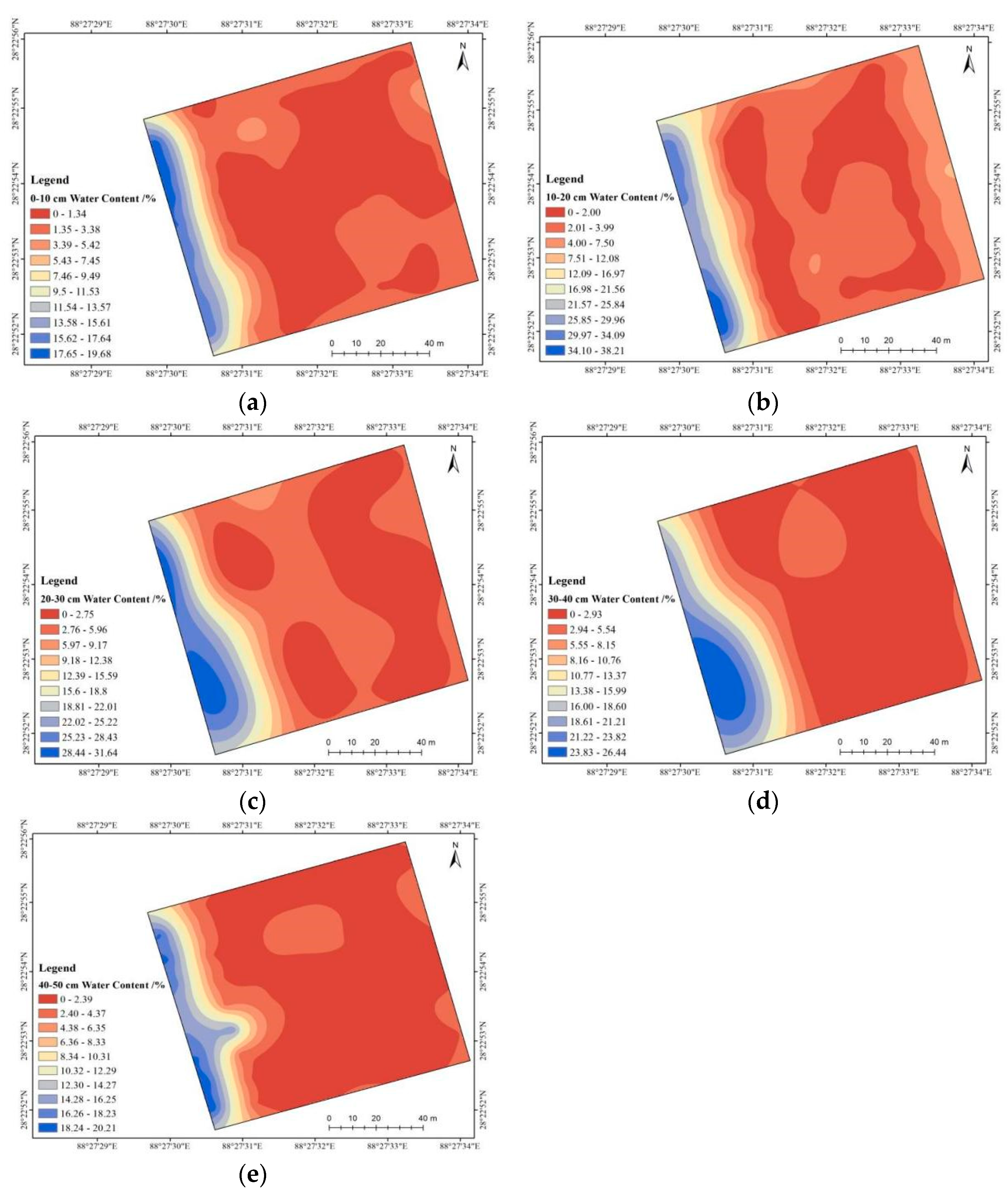
3.2. Spatial Heterogeneity of Soil Moisture in the Alpine Valley Desert

The structural parameters of three semi-variance function models are shown in Table 3. The optimal semi-variance function model for soil gravimetric water content in the 0–10 cm soil layer is determined as the Spherical model, and that for soil gravimetric water content in the 10–20 and 40–50 cm soil layers is selected as the Exponential model. The optimal theoretical model for soil gravimetric water content in the 20–30 and 30–40 cm soil layers is confirmed as the Gaussian model.
The nugget values of the different soil layers are between 0.1 and 0.34, the nugget value of the 10–20 cm soil layer is the smallest, and that of the 20–30 cm soil layer is the largest. This finding indicates that the spatial heterogeneity is smallest and largest in the 10–20 and 20–30 cm soil layers, respectively. The sill value of the dune soil first increases and then decreases with the increase in soil depths. The 0–30 cm layer is greatly affected by the elevation of the soil, while the 30–50 cm layer is weakened by the elevation. The different elevations affect the growth and distribution of vegetation in different soil layers of dunes, thus impacting the spatial distribution of soil moisture.
From Table 3, the nugget coefficients are 13.7% in the 0–10 cm, 0.1% in the 10–20 cm, 22.8% in the 20–30 cm, 26.4% in the 30–40 cm, and 13.4% in the 40–50 cm layer. This result indicates that the soil gravimetric water content in the 30–40 cm soil layer of the dune has a moderate spatial correlation, whereas the soil gravimetric water content in other soil layers has a strong spatial correlation. The spatial correlation of the 10–20 cm soil layer is stronger than those of the other soil layers. The range of soil gravimetric water content varies from 31.23 to 63.38 m, and is greater than the minimum sampling interval of this study (15 m). This finding suggests that the sample design is sufficient to reflect the entire sample soil moisture content of the spatial structure characteristics.
To describe the spatial distribution of soil gravimetric water content intuitively, the optimal semi-variance function model and its characteristic parameters in Table 3 were selected to draw spatial distribution maps of soil gravimetric water content at different levels through the Kriging interpolation, as shown in Figure 3. The spatial distribution of soil gravimetric water content in different soil layers is mostly patched and banded. The spatial distribution of soil gravimetric water content in the sampling points is higher in the southwest than in other areas. The dune elevation gradually increases from the southwest to the northeast parts. Conversely, the soil gravimetric water content declines from the bottom of the windward slope to the top of the dune. In the 0–10, 10–20, and 20–30 cm soil layers, the soil gravimetric water content presents a banded and patchy distribution, which can reflect the soil gravimetric water content heterogeneity of different parts (Figure 3).
Table 4 shows the correlation matrix of soil gravimetric water content at different layers based on Pearson correlation analysis. There is a high similarity observed among the layers of soil moisture. The soil gravimetric water content presents an extremely significant correlation among different depths (p < 0.01). In most cases, the correlation of soil gravimetric water content gradually decreases with the increase in soil depths.

3.3. Driving Factors of Soil Moisture in Alpine Valley Dunes

3.3.1. Factor Detector

The geographical detector can explain the influence of each factor on the change in soil moisture content in the dune. Table 5 shows the q values of evaluation factors. The ranking of the influence of the evaluation factors on the alpine valley dune is elevation > slope > location > vegetation > aspect.
The q values of elevation, slope, and vegetation coverage increase with depth. This result implies that these factors are the main influencing factors of soil gravimetric water content variation at different depths of the dune. The q values of the slope aspect do not exceed 0.05, indicating that the aspect has a minimal influence on the variability in soil gravimetric water content at different depths of the dune.

3.3.2. Interactive Detector

Table 6 indicates the evaluation factor interaction detection. The evaluation factors influence the soil gravimetric water content of the dune. An interaction was determined among the evaluation factors, but no independent factors were found. In the 0–10 cm soil layer, 60% of the evaluation factor interaction combinations show a two-factor enhancement relationship, and 40% present a nonlinear enhancement relationship (Appendix A). The most influential interactions were the dune location and elevation combination (0.8901), elevation and aspect combination (0.8901), elevation and slope combination (0.8901), and elevation and vegetation coverage combination (0.8834). The combination of slope aspect and vegetation coverage was less influential (0.5154).
In the 10–20 cm soil layer, 90% of the evaluation factor interaction combinations show a two-factor enhancement relationship, and 10% demonstrate a nonlinear enhancement relationship. The interaction influence is relatively considerable. The greatest combinations were position and elevation (0.9124), elevation and aspect (0.9124), and elevation and slope (0.9124). The slope aspect and vegetation combination was minimum (0.6880).
In the 20–30 cm soil layer, the interaction combination of evaluation factors shows a two-factor enhancement relationship. The influence of interaction is relatively remarkable. The strongest combinations were position and elevation (0.9288), elevation and aspect (0.9288), and elevation and slope (0.9288), and the weakest combination was slope aspect and vegetation (0.6880). In the 30–40 cm soil layer, the interaction combination of slope aspect and vegetation combination (0.7208) shows a nonlinear enhancement relationship, whereas the interaction combinations of other evaluation factors indicate a two-factor enhancement relationship. The influences of interaction were between 0.7891 and 0.9560.
In the 40–50 cm soil layer, 60% of the evaluation factor interaction combinations show a two-factor enhancement relationship, and the interaction influence was between 0.7423 and 0.9300. Among the evaluation factor interaction combinations, 40% show a nonlinear enhancement relationship, and the interaction influences were 0.6210–0.9300. In the 0–50 cm soil layer, 70% of the evaluation factor interaction combinations show a two-factor enhancement relationship, and 30% show a nonlinear enhancement relationship. The interaction among evaluation factors has a strong effect of dual factors and a nonlinear enhancement effect on soil gravimetric water content (Appendix A).

3.3.3. Ecological Detector

Ecological detection can be used to compare whether a significant difference exists between two factors on the independent variable of soil water change. In Table 6, “Y” means that a significant difference exists between the row factor and the column factor, and “N” means that no significant difference exists between them. The factor combinations in different soil layers have distinct significant effects on soil moisture changes. Among the factor combinations in the 0–10, 20–30, and 30–40 cm soil layers, 70% have significant differences in soil moisture changes, but no significant difference exists between position and slope, position and vegetation, and slope and vegetation combinations. In the 10–20, 40–50, and 0–50 cm soil layers, 90% of factor combinations have significant differences in soil gravimetric water content changes, but no significant difference exists in the positions and slope of these three soil layers.

4. Discussion

The influencing factors of soil gravimetric water content are mainly natural and human factors, but most of the Qinghai–Tibet Plateau is dominated by natural factors [38]. Among the natural factors, the primary driver of the vegetation coverage factor is soil gravimetric water content [35]. In a previous study on soil gravimetric water content, the influence of climate factors on soil moisture is mainly reflected in the difference between water infiltration and evapotranspiration caused by rainfall and solar radiation [39]. Under certain conditions, the local climate has an important influence on the spatial-temporal pattern of soil gravimetric water content, due to the differences in rainfall and temperature at different elevations, which may be an important factor affecting the soil water pattern [40]. On a small scale, soil types, topographic factors, and vegetation factors are the main factors affecting the soil water pattern; on a large scale, climatic factors, such as rainfall and evapotranspiration, are the main factors controlling the soil water pattern [24]. The impacts of soil types, vegetation factors, and topographic factors on soil water are generally consistent with depth, such that the variation in deep soil water mainly depends on soil types, vegetation, and topographic factors [2,35,41,42,43]. Therefore, the factors adopted in this study are mainly different dune locations, vegetation, elevation, aspect, and slope.
Many studies have also verified the special effect of vegetation cover on soil properties in the Tibetan Plateau [42,43]. Some scholars have conducted research to assess the spatial variability of soil gravimetric water content and the temporal and spatial variations in a typical alpine meadow in the Qinghai–Tibet Plateau by using a geostatistical approach. Studies on soil moisture in the Qinghai–Tibet Plateau have mainly focused on the following four aspects: (1) inversion of surface soil moisture by using remote sensing images, (2) spatial-temporal changes of soil temperature and humidity, (3) model simulation of hydrothermal characteristics, and (4) the impacts of soil moisture and physical properties. In this study, the ranking of the influence of each evaluation factor on the alpine dune was elevation > slope > location > vegetation > aspect. This result is different from that in the Loess Plateau (location on the hill slope, vegetation cover, slope, relative elevation, and sine of the aspect) [14]. This difference may be caused by harsh climate conditions and diverse natural landscapes under an average elevation of 4505 m. The results of this study can be compared with those in other arid regions. The differences in soil moisture in various regions can be clearly compared, providing research guidance for subsequent studies.
Compared with the previous studies, such as those of [35] and [44], the spatial heterogeneity of soil gravimetric water content in an alpine desert is higher than that in alpine meadows and shrubs. This condition depends mainly on the capability of soil water conservation and the sensitivity of vegetation cover to precipitation and perched aquifer. If the sample area is extremely small, it cannot contain all information to reflect the spatial heterogeneity of the entire community. If the sample plot is exceedingly large, the difference in variables among sample plots will disappear [38]. Certain scale and zoning effects occur in the selection of sample plots. This issue was also found in this study. Thus, selecting the size of sample plots and determining the direction of the plots are important in the spatial heterogeneity research of soil water.
According to the classification by coefficient of variation, the coefficient of variation less than 10% is weak variability, and that of 10–100% is moderate variability, while the coefficient of variation larger than 100% is strong variability [45]. In this study, the variation coefficients of soil gravimetric water content in different soil layers were between 130% and 169%, showing the strong variability. This may be affected by vegetation and topographic factors, as well as extreme rainfall, sand movement, strong evaporation, and groundwater table fluctuation, which is consistent with the conclusion of Li et al. [33]. Moreover, the uncertainty resulting from the random measured samples may increase such strong soil moisture variability [13,33,46]. In the geographical detector analysis, the interaction among evaluation factors had a strong effect of dual factors and a nonlinear enhancement effect on soil gravimetric water content in the 0–50 cm layer. This implies that there are no independent factors existing in the impacts of soil gravimetric water content [21].
In general, this study is of great significance to assess the soil water status in alpine desert regions. It provides basic research for artificial vegetation restoration and regeneration and soil structure analysis of different desert types in alpine cold regions. The current study applied a geographical detector to examine the influence of different factors on soil moisture and the interaction factors in a relatively small area. Owing to the harsh field conditions in the Qinghai–Tibet Plateau area, analysis of soil moisture through point distribution, drilling, and other methods requires time and effort. In the future study, remote sensing data are urgently needed to retrieve measurements of soil water, such that the spatial distribution of soil water in a large area can be verified.

5. Conclusions

Based on soil sample collection, combined with geostatistical analysis and a geographical detector method, this study detected the spatial heterogeneity and driving factors of soil gravimetric water content in typical alpine valley dunes of the Qinghai–Tibet Plateau. The results showed that the average value of soil gravimetric water content at different depths ranged from 3.68% to 7.84%. The coefficient of variation indicated that the soil moisture content in different soil layers of the sample plot shows strong variability.
The optimal theoretical models of soil gravimetric water content in 0–50 cm layers of dunes were different. The nugget coefficient shows that the soil gravimetric water content in the dune has a strong spatial correlation, and the range of the optimal theoretical model of semi-variance function was 31.23–63.38 m, which is much larger than the 15 m sampling distance. The ranking of the influence of each evaluation factor on the alpine dune was elevation > slope > location > vegetation > aspect.
The correlation analysis of soil gravimetric water content in different soil layers showed a significant correlation (p < 0.01). The interaction detection of factors indicated an interaction among evaluation factors, and no factors were independent of one another. In each soil layer of 0–50 cm, the interaction among evaluation factors had a strong dual effect and a nonlinear enhancement effect on soil gravimetric water content. The significance analysis of ecological detection indicated significant differences among the factor combinations of different soil layers on soil water change. In general, the analyses of spatial distribution, heterogeneity, and driving factors of soil gravimetric water content have implications for understanding the spatial heterogeneity and driving factors of soil moisture, and guiding artificial vegetation restoration and soil structure analysis of different desert types in alpine cold desert regions. The remote sensing data is urgently recommended to retrieve measurements of soil gravimetric water content in a large area for the vegetation restoration of alpine cold regions in further work.

Author Contributions

Conceptualization, Z.Z., H.Y. and J.X.; methodology, H.Y., J.H. and B.Y.; formal analysis, H.Y., J.H. and B.Y.; writing—original draft preparation, Z.Z.; writing—review and editing, Y.Z., S.W. and J.X. All authors have read and agreed to the published version of the manuscript.

Funding

This research was financially supported by the Investigation on resource environment and biodiversity of typical mountainous areas in different climatic zones (2019FY101601-2), the original innovation project of the basic frontier scientific research program, Chinese Academy of Sciences (ZDBS-LY-DQC031), the National Natural Science Foundation of China (42071259), the Natural Science Foundation of Tibet Autonomous Region (XZ2019ZR G-61), Natural Science Foundation of Xinjiang Uygur Autonomous Region (2021D01E01), the Young Talent Growth Fund Project of Northwest Institute of Ecological Environment and Resources, Chinese Academy of Sciences (FEYS2019016), and the Youth Innovation Promotion Association of the Chinese Academy of Sciences (2019430).

Institutional Review Board Statement

Not applicable.

Informed Consent Statement

Not applicable.

Data Availability Statement

The data is available from the corresponding author upon reasonable request.

Conflicts of Interest

The authors declare no conflict of interest.

Appendix A

Table A1. Evaluation Factor Interaction Results.
Soil Depth
/cm
Interaction (C)Sum of q ValuesResultInfluence
0–10X1 ∩ X2 = 0.89011.5017 C > Max(q (X1), q (X2))Two-factor enhancement
X1 ∩ X3 = 0.62670.6209 C > Max(q (X1), q (X2))Nonlinear enhancement
X1 ∩ X4 = 0.62671.2406 C > q (X1) + q (X4)Two-factor enhancement
X1 ∩ X5 = 0.62671.0981 C > Max(q (X1), q (X4))Two-factor enhancement
X2 ∩ X3 = 0.89010.8820 C > Max(q (X1), q (X5))Nonlinear enhancement
X2 ∩ X4 = 0.89011.5017 C > q (X2) + q (X4)Two-factor enhancement
X2 ∩ X5 = 0.88341.3592 C > Max(q (X2), q (X4))Two-factor enhancement
X3 ∩ X4 = 0.62670.6209 C > Max(q (X2), q (X5))Nonlinear enhancement
X3 ∩ X5 = 0.51540.4784 C > q (X3) + q (X5)Nonlinear enhancement
X4 ∩ X5 = 0.62671.0981 C > q (X4) + q (X5)Two-factor enhancement
10–20X1 ∩ X2 = 0.91241.7320 C > Max(q (X4), q (X5))Two-factor enhancement
X1 ∩ X3 = 0.82650.8583 C > Max(q (X1), q (X2))Two-factor enhancement
X1 ∩ X4 = 0.82651.6470 C > Max(q (X1), q (X3))Two-factor enhancement
X1 ∩ X5 = 0.82671.4510 C > Max(q (X1), q (X4))Two-factor enhancement
X2 ∩ X3 = 0.91240.9433 C > Max(q (X1), q (X5))Two-factor enhancement
X2 ∩ X4 = 0.91241.7320 C > Max(q (X2), q (X3))Two-factor enhancement
X2 ∩ X5 = 0.91001.5360 C > Max(q (X2), q (X4))Two-factor enhancement
X3 ∩ X4 = 0.82650.8583 C > Max(q (X2), q (X5))Two-factor enhancement
X3 ∩ X5 = 0.76980.6623 C > Max(q (X3), q (X4))Nonlinear enhancement
X4 ∩ X5 = 0.82671.4510 C > q (X4) + q (X5)Two-factor enhancement
20–30X1 ∩ X2 = 0.92881.6646 C > Max(q (X4), q (X5))Two-factor enhancement
X1 ∩ X3 = 0.74150.7648 C > Max(q (X1), q (X2))Two-factor enhancement
X1 ∩ X4 = 0.74151.4742 C > Max(q (X1), q (X3))Two-factor enhancement
X1 ∩ X5 = 0.74171.4192 C > Max(q (X1), q (X4))Two-factor enhancement
X2 ∩ X3 = 0.92880.9552 C > Max(q (X1), q (X5))Two-factor enhancement
X2 ∩ X4 = 0.92881.6646 C > Max(q (X2), q (X3))Two-factor enhancement
X2 ∩ X5 = 0.92871.6096 C > Max(q (X2), q (X4))Two-factor enhancement
X3 ∩ X4 = 0.74150.7648 C > Max(q (X2), q (X5))Two-factor enhancement
X3 ∩ X5 = 0.68800.7098 C > Max(q (X3), q (X4))Two-factor enhancement
X4 ∩ X5 = 0.74171.4192 C > Max(q (X3), q (X5))Two-factor enhancement
30–40X1 ∩ X2 = 0.95601.7390 C > Max(q (X4), q (X5))Two-factor enhancement
X1 ∩ X3 = 0.78910.7930 C > Max(q (X1), q (X2))Two-factor enhancement
X1 ∩ X4 = 0.78911.5710 C > Max(q (X1), q (X3))Two-factor enhancement
X1 ∩ X5 = 0.78911.4881 C > Max(q (X1), q (X4))Two-factor enhancement
X2 ∩ X3 = 0.95600.9610 C > Max(q (X1), q (X5))Two-factor enhancement
X2 ∩ X4 = 0.95601.7390 C > Max(q (X2), q (X3))Two-factor enhancement
X2 ∩ X5 = 0.95421.6561 C > Max(q (X2), q (X4))Two-factor enhancement
X3 ∩ X4 = 0.78910.7930 C > Max(q (X2), q (X5))Two-factor enhancement
X3 ∩ X5 = 0.72080.7101 C > Max(q (X3), q (X4))Nonlinear enhancement
X4 ∩ X5 = 0.78911.4881 C > q (X4) + q (X5)Two-factor enhancement
40–50X1 ∩ X2 = 0.93001.6661 C > Max(q (X4), q (X5))Two-factor enhancement
X1 ∩ X3 = 0.74230.7382 C > Max(q (X1), q (X2))Nonlinear enhancement
X1 ∩ X4 = 0.74231.4760 C > q (X1) + q (X4)Two-factor enhancement
X1 ∩ X5 = 0.74261.3299 C > Max(q (X1), q (X4))Two-factor enhancement
X2 ∩ X3 = 0.93000.9283 C > Max(q (X1), q (X5))Nonlinear enhancement
X2 ∩ X4 = 0.93001.6661 C > q (X2) + q (X4)Two-factor enhancement
X2 ∩ X5 = 0.92931.5200 C > Max(q (X2), q (X4))Two-factor enhancement
X3 ∩ X4 = 0.74230.7382 C > Max(q (X2), q (X5))Nonlinear enhancement
X3 ∩ X5 = 0.62100.5921 C > q (X3) + q (X5)Nonlinear enhancement
X4 ∩ X5 = 0.74261.3299 C > q (X4) + q (X5)Two-factor enhancement
0–50X1 ∩ X2 = 0.98111.8660 C > Max(q (X4), q (X5))Two-factor enhancement
X1 ∩ X3 = 0.88730.8859 C > Max(q (X1), q (X2))Nonlinear enhancement
X1 ∩ X4 = 0.88731.7706 C > q (X1) + q (X4)Two-factor enhancement
X1 ∩ X5 = 0.88731.6609 C > Max(q (X1), q (X4))Two-factor enhancement
X2 ∩ X3 = 0.98110.9813 C > Max(q (X1), q (X5))Two-factor enhancement
X2 ∩ X4 = 0.98111.8660 C > Max(q (X2), q (X3))Two-factor enhancement
X2 ∩ X5 = 0.98101.7563 C > Max(q (X2), q (X4))Two-factor enhancement
X3 ∩ X4 = 0.88730.8859 C > Max(q (X2), q (X5))Nonlinear enhancement
X3 ∩ X5 = 0.81270.7762 C > q (X3) + q (X5)Nonlinear enhancement
X4 ∩ X5 = 0.88731.6609 C > q (X4) + q (X5)Two-factor enhancement

References

  1. Li, X.; Shao, M.; Zhao, C.; Jia, X. Spatial variability of soil water content and related factors across the Hexi Corridor of China. J. Arid. Land 2019, 11, 123–134. [Google Scholar] [CrossRef] [Green Version]
  2. Bi, H.; Li, X.; Liu, X.; Guo, M.; Li, J. A case study of spatial heterogeneity of soil moisture in the Loess Plateau, western China: A geostatistical approach. Int. J. Sediment Res. 2009, 24, 63–73. [Google Scholar] [CrossRef]
  3. Seneviratne, S.I.; Corti, T.; Davin, E.; Hirschi, M.; Jaeger, E.B.; Lehner, I.; Orlowsky, B.; Teuling, A. Investigating soil moisture–climate interactions in a changing climate: A review. Earth-Sci. Rev. 2010, 99, 125–161. [Google Scholar] [CrossRef]
  4. McColl, K.A.; Alemohammad, S.H.; Akbar, R.; Konings, A.G.; Yueh, S.; Entekhabi, D. The global distribution and dynamics of surface soil moisture. Nat. Geosci. 2017, 10, 100–104. [Google Scholar] [CrossRef]
  5. Moore, G.W.; Jones, J.A.; Bond, B.J. How soil moisture mediates the influence of transpiration on streamflow at hourly to interannual scales in a forested catchment. Hydrol. Process. 2011, 25, 3701–3710. [Google Scholar] [CrossRef]
  6. Jia, X.; Zhu, Y.; Luo, Y. Soil moisture decline due to afforestation across the Loess Plateau, China. J. Hydrol. 2017, 546, 113–122. [Google Scholar] [CrossRef]
  7. Venkatesh, B.; Lakshman, N.; Purandara, B.K.; Reddy, V.B. Analysis of observed soil moisture patterns under different land coversin Western Ghats, India. J. Hydrol. 2011, 397, 281–294. [Google Scholar] [CrossRef]
  8. Wei, X.; Zhou, Q.; Cai, M.; Wang, Y. Effects of Vegetation Restoration on Regional Soil Moisture Content in the Humid Karst Areas—A Case Study of Southwest China. Water 2021, 13, 321. [Google Scholar] [CrossRef]
  9. Baroni, G.; Ortuani, B.; Facchi, A.; Gandolfi, C. The role of vegetation and soil properties on the spatio-temporal variability of the surface soil moisture in a maize-cropped field. J. Hydrol. 2013, 489, 148–159. [Google Scholar] [CrossRef]
  10. Neelam, M.; Mohanty, B. On the Radiative Transfer Model for Soil Moisture across Space, Time and Hydro-Climates. Remote Sens. 2020, 12, 2645. [Google Scholar] [CrossRef]
  11. Zhang, W.; Yi, S.; Qin, Y.; Sun, Y.; Shangguan, D.; Meng, B.; Li, M.; Zhang, J. Effects of Patchiness on Surface Soil Moisture of Alpine Meadow on the Northeastern Qinghai-Tibetan Plateau: Implications for Grassland Restoration. Remote Sens. 2020, 12, 4121. [Google Scholar] [CrossRef]
  12. Herbert, C.; Pablos, M.; Vall-Llossera, M.; Camps, A.; Martínez-Fernández, J. Analyzing Spatio-Temporal Factors to Estimate the Response Time between SMOS and In-Situ Soil Moisture at Different Depths. Remote. Sens. 2020, 12, 2614. [Google Scholar] [CrossRef]
  13. Guo, X.; Fu, Q.; Hang, Y.; Lu, H.; Gao, F.; Si, J. Spatial Variability of Soil Moisture in Relation to Land Use Types and Topographic Features on Hillslopes in the Black Soil (Mollisols) Area of Northeast China. Sustainability 2020, 12, 3552. [Google Scholar]
  14. Feng, Q.; Zhao, W.; Qiu, Y.; Zhao, M.; Zhong, L. Spatial Heterogeneity of Soil Moisture and the Scale Variability of Its Influencing Factors: A Case Study in the Loess Plateau of China. Water 2013, 5, 1226–1242. [Google Scholar]
  15. Zhu, Q.; Lin, H. Influences of soil, terrain, and crop growth on soil moisture variation from transect to farm scales. Geoderma 2011, 163, 45–54. [Google Scholar] [CrossRef]
  16. Lakhankar, T.; Ghedira, H.; Temimi, M.; Azar, A.E.; Khanbilvardi, R. Effect of Land Cover Heterogeneity on Soil Moisture Retrieval Using Active Microwave Remote Sensing Data. Remote. Sens. 2009, 1, 80–91. [Google Scholar] [CrossRef] [Green Version]
  17. Li, H.; Shen, W.; Zou, C.; Jiang, J.; Fu, L.; She, G. Spatio-temporal variability of soil moisture and its effect on vegetation in a desertified aeolian riparian ecotone on the Tibetan Plateau, China. J. Hydrol. 2013, 479, 215–225. [Google Scholar] [CrossRef]
  18. López-Vicente, M.; Quijano, L.; Navas, A. Spatial patterns and stability of topsoil water content in a rainfed fallow cereal field and Calcisol-type soil. Agric. Water Manag. 2015, 161, 41–52. [Google Scholar] [CrossRef] [Green Version]
  19. Delbari, M.; Afrasiab, P.; Gharabaghi, B.; Amiri, M.; Salehian, A. Spatial variability analysis and mapping of soil physical and chemical attributes in a salt-affected soil. Arab. J. Geosci. 2019, 12, 68. [Google Scholar]
  20. Arriaga, J.; Rubio, F.R. A distributed parameters model for soil water content: Spatial and temporal variability analysis. Agric. Water Manag. 2017, 183, 101–106. [Google Scholar] [CrossRef]
  21. Wang, J.F.; Li, X.H.; Christakos, G.; Liao, Y.L.; Zhang, T.; Gu, X.; Zheng, X.Y. Geographical detectors-based health risk assessment and its application in the neural tube defects study of the Heshun region, China. Int. J. Geogr. Inf. Sci. 2010, 24, 107–127. [Google Scholar] [CrossRef]
  22. Du, J.; Yang, Z.G. Tibet Autonomous Region County-Level Climate Regionalization; China Meteorological Press: Beijing, China, 2013; pp. 73–74. [Google Scholar]
  23. Prokopovich, N.P.; Bara, J.P. Soil classification system, unified. In Applied Geology; Finkl, C., Ed.; Encyclopedia of Earth Sciences Series; Springer: Boston, MA, USA, 1984; Volume 3. [Google Scholar]
  24. Entin, J.K.; Robock, A.; Vinnikov, K.Y.; Hollinger, S.E.; Liu, S.; Namkhai, A. Temporal and spatial scales of observed soil moisture variations in the extratropics. J. Geophys. Res. Atmos. 2000, 105, 11865–11877. [Google Scholar] [CrossRef]
  25. Woebbecke, D.M. Plant species identification, size, and enumeration using machine vision techniqueson near-binary images. Proc. SPIE 1993, 1836, 208–219. [Google Scholar]
  26. Ren, J.; Bai, Y.C.; Wang, J.D. An efficient method for extracting vegetation coverage from digital photographs. Remote Sens. Technol. Appl. 2010, 25, 719–724. [Google Scholar]
  27. Journel, A.G. Mining Geostatistics; Academic Press: New York, NY, USA, 1978. [Google Scholar]
  28. Li, H.; Reynolds, J.F. On Definition and Quantification of Heterogeneity. Oikos 1995, 73, 280–284. [Google Scholar] [CrossRef]
  29. Maroufpoor, S.; Bozorg-Haddad, O.; Chu, X.F. Chapter 9—Geostatistics: Principles and Methods. In Handbook of Probabilistic Models; Samui, P., Bui, D.T., Chakraborty, S., Ravinesh, C.D., Eds.; Butterworth-Heinemann: Oxford, UK, 2020; pp. 229–242. [Google Scholar]
  30. Jean-Paul, C.; Pierre, D. Geostatistics: Modeling Spatial Uncertainty; Jhon Wiley & Sons Inc.: New York, NY, USA, 1999; p. 695. [Google Scholar]
  31. Paramasivam, C.; Venkatramanan, S. An Introduction to Various Spatial Analysis Techniques. GIS Geostat. Tech. Groundw. Sci. 2019, 23–30. [Google Scholar] [CrossRef]
  32. Zhang, Y.; Zhang, K.-C.; An, Z.-S.; Yu, Y.-P. Quantification of driving factors on NDVI in oasis-desert ecotone using geographical detector method. J. Mt. Sci. 2019, 16, 2615–2624. [Google Scholar] [CrossRef]
  33. Li, H.; Shen, W.; Lin, N.; Yuan, L.; Sun, M.; Ji, D. Spatial variability of soil moisture on aeolian sandy land in riparian ecotone of middle reaches of yarlung zangbo river valley. Trans. Chin. Soc. Agric. Eng. 2012, 28, 150–155. [Google Scholar]
  34. Liu, B.; Zhao, W.; Zeng, F. Statistical analysis of the temporal stability of soil moisture in three desert regions of northwestern China. Env. Earth Sci. 2013, 70, 2249–2262. [Google Scholar] [CrossRef]
  35. Zhu, X.; Shao, M.; Liang, Y.; Tian, Z.; Wang, X.; Qu, L. Mesoscale spatial variability of soilâ water content in an alpine meadow on the northern Tibetan Plateau. Hydrol. Process. 2019, 33, 2523–2534. [Google Scholar] [CrossRef]
  36. Zhang, X.; Zhao, Y. Identification of the driving factors’ influences on regional energy-related carbon emissions in China based on geographical detector method. Environ. Sci. Pollut. Res. 2018, 25, 9626–9635. [Google Scholar] [CrossRef]
  37. Conover, W.J.; Conover, W.J. Practical Nonparametric Statistics; John Wiley & Sons: Hoboken, NJ, USA, 1980. [Google Scholar]
  38. Liu, L.J.; Zhang, H.; Luo, L. Spatial heterogeneity of soil water of alpine area in eastern Qinghai-tibet plateau. J. Wuhan Univ. 2008, 54, 414–420. [Google Scholar]
  39. Savva, Y.; Szlavecz, K.; Carlson, D.; Gupchup, J.; Szalay, A.; Terzis, A. Spatial patterns of soil moisture under forest and grass land cover in a suburban area, in Maryland, USA. Geoderma 2013, 192, 202–210. [Google Scholar] [CrossRef]
  40. Wang, Y.; Shao, M.; Liu, Z. Vertical distribution and influencing factors of soil water content within 21-m profile on the Chinese Loess Plateau. Geoderma 2013, 300–310. [Google Scholar] [CrossRef]
  41. Zhu, Q.; Nie, X.; Zhou, X.; Liao, K.; Li, H. Soil moisture response to rainfall at different topographic positions along a mixed land-use hillslope. Catena 2014, 119, 61–70. [Google Scholar] [CrossRef]
  42. Yang, R.M.; Zhang, G.L.; Yang, F.; Zhi, J.J.; Yang, F.; Liu, F.; Zhao, Y.G.; Li, D.C. Precise estimation of soil organic carbon stocks in the northeast Tibetan Plateau. Sci. Rep. 2016, 6, 21842. [Google Scholar] [CrossRef] [PubMed] [Green Version]
  43. Zeng, C.; Zhang, F.; Wang, Q.; Chen, Y.; Joswiak, D.R. Impact of alpine meadow degradation on soil hydraulic properties over the Qinghai-Tibetan Plateau. J. Hydrol. 2013, 478, 148–156. [Google Scholar] [CrossRef]
  44. Yang, Z.; Ouyang, H.; Zhang, X.; Xu, X.; Zhou, C.; Yang, W. Spatial variability of soil moisture at typical alpine meadow and steppe sites in the Qinghai-Tibetan Plateau permafrost region. Environ. Earth Sci. 2010, 63, 477–488. [Google Scholar] [CrossRef] [Green Version]
  45. Li, H. A Study on Spatial Variability of Soil Properties and Influence of Vegetation on It at a Catchment of Southern Jiangsu Province in China; Nanjing Forestry University: Nanjing, China, 2008; (In Chinese with English Abstract). [Google Scholar]
  46. Yang, Y.; Huang, Y.; Zhang, Y.; Tong, X. Optimal Irrigation Mode and Spatio-Temporal Variability Characteristics of Soil Moisture Content in Different Growth Stages of Winter Wheat. Water 2018, 10, 1180. [Google Scholar] [CrossRef] [Green Version]
Figure 1. Overview of the study area. (a) location and distribution of soil sampling points, (b) annual mean temperature and annual precipitation, (c) soil bulk density in the study area.
Water 13 02652 g001
Figure 2. (a) Sketch of the planform of measuring positions on a sand dune (a = 100 m) and (b) sampling location of the dune: A is the middle part of the leeward slope, B is the top, C is the middle and upper part of the windward slope, D is the middle part of the windward slope, E is the middle and lower part of the windward slope, F is the bottom part of the windward slope, and G is the interdune land.
Water 13 02652 g002
Figure 3. Spatial distribution of soil moisture in different soil layers. (a) soil gravimetric water content at 0–10 cm layer, (b) soil gravimetric water content at 10–20 cm layer, (c) soil gravimetric water content at 20–30 cm layer, (d) soil gravimetric water content at 30–40 cm layer, (e) soil gravimetric water content at 40–50 cm layer.
Water 13 02652 g003
Table 1. Types of interaction between two factors [21,32,36].
InteractionDescription
Weaken, nonlinear q ( X 1 X 2 )   <   Min   ( q ( X 1 ) ,   q ( X 2 ) )
Weaken, univariate Min ( q ( X 1 ) ,   q ( X 2 ) )   <   q ( X 1 X 2 ) <   Max   ( q ( X 1 ) , q ( X 2 ) )
Enhance, bivariate q ( X 1 X 2 ) > Max   ( q ( X 1 ) , q ( X 2 ) )
Independent q ( X 1 X 2 ) = q ( X 1 ) + q ( X 2 )
Enhance, nonlinear q ( X 1 X 2 ) > q ( X 1 ) + q ( X 2 )
Table 2. Descriptive statistics of soil moisture at different layers.
Depth
/cm
Minimum
/%
Maximum
/%
Mean
/%
Standard DeviationVariation
/%
KurtosisSkewnessK-S Test
Z Value *p Value *Z Value #p Value #
0–100.0720.933.686.231692.532.020.3400.820.54
10–200.2738.337.0610.711522.932.110.3500.830.40
20–300.5133.037.8410.281310.771.550.3500.800.24
30–400.5928.856.638.601300.531.490.3600.800.31
40–500.2621.614.366.351462.261.990.3700.790.42
Note: Z value represents the Z-statistic of the K-S test, p value is the corresponding probability, and p > 0.05 means a normal distribution. * and # respectively refer to the statistical results of the original and logarithmic soil gravimetric water contents.
Table 3. Theoretical semi-variogram models of soil moisture and its related parameters.
Depth
/cm
Theoretical ModelNuggetSillNugget Coefficient
/%
Range
/m
Coefficient of DeterminationResidual Sum of Squares (%2)
0–10Spherical model6.3045.9913.737.420.9913.98
Exponential model2.4045.85.2044.610.989.49
Gaussian model10.7341.9825.6027.310.979.99
10–20Spherical model14.90111.923.3023.510.96110
Exponential model0.10124.10.1031.230.9843.60
Gaussian model25108.602317.580.96110
20–30Spherical model20.6016912.2061.090.9697.70
Exponential model17.90236.707.60142.280.95150
Gaussian model34148.9022.8041.700.9921.20
30–40Spherical model2010119.8045.990.92142
Exponential model17.6096.2018.3071.010.87180
Gaussian model28.5010826.4046.190.9750.60
40–50Spherical model9.3740.783223.760.98344.20
Exponential model7.2053.6413.4063.380.990.37
Gaussian model13.4540.0533.6023.480.995.15
Table 4. Correlation matrix of soil moisture at different layers.
Soil Depth/cm0–1010–2020–3030–4040–50
0–101
10–200.953 **1
20–300.890 **0.858 **1
30–400.820 **0.796 **0.970 **1
40–500.898 **0.926 **0.862 **0.816 **1
Note: ** refers to a significant correlation at the 0.01 level (bilateral).
Table 5. q values of evaluation factors.
Soil Depth/cmNatural FactorsLocationElevationAspectSlopeVegetation
0–10q 0.620 0.881 0.001 0.620 0.478
p value0.0000.430 0.859 0.0000.000
10–20q 0.824 0.909 0.035 0.824 0.628
p value0.0000.243 0.342 0.0000.000
20–30q 0.737 0.928 0.028 0.737 0.682
p value0.0000.137 0.222 0.0000.000
30–40q 0.785 0.953 0.008 0.785 0.703
p value0.0000.021 0.543 0.0000.000
40–50q 0.738 0.928 0.000 0.738 0.592
p value0.0000.109 0.926 0.0000.000
0–50q 0.885 0.981 0.001 0.885 0.776
p value0.0000.0000.879 0.0000.000
Table 6. Evaluation factor interaction detection.
Soil Depth
/cm
IndexLocationElevationAspectSlopeVegetation
X1X2X3X4X5
0–10X10.6203
X20.8901 (Y)0.8814
X30.6267 (Y)0.8901 (Y)0.0006
X40.6267 (N)0.8901 (Y)0.6267 (Y)0.6203
X50.6267 (N)0.8834 (Y)0.5154 (Y)0.6267 (N)0.4778
10–20X10.8235
X20.9124 (Y)0.9085
X30.8265 (Y)0.9124 (Y)0.0348
X40.8265 (N)0.9124 (Y)0.8265 (Y)0.8235
X50.8267 (Y)0.9100 (Y)0.7698 (Y)0.8267 (Y)0.6275
20–30X10.7371
X20.9288 (Y)0.9275
X30.7415 (Y)0.9288 (Y)0.0277
X40.7415 (N)0.9288 (Y)0.7415 (Y)0.7371
X50.7417 (N)0.9287 (Y)0.6880 (Y)0.7417 (N)0.6821
30–40X10.7855
X20.9560 (Y)0.9535
X30.7891 (Y)0.9560 (Y)0.0075
X40.7891 (N)0.9560 (Y)0.7891 (Y)0.7855
X50.7891 (N)0.9542 (Y)0.7208 (Y)0.7891 (N)0.7026
40–50X10.7380
X20.9300 (Y)0.9281
X30.7423 (Y)0.9300 (Y)0.0002
X40.7423 (N)0.9300 (Y)0.7423 (Y)0.7380
X50.7426 (Y)0.9293 (Y)0.6210 (Y)0.7426 (Y)0.5919
0–50X10.8853
X20.9811 (Y)0.9807
X30.8873 (Y)0.9811 (Y)0.0006
X40.8873 (N)0.9811 (Y)0.8873 (Y)0.8853
X50.8873 (Y)0.9810 (Y)0.8127 (Y)0.8873 (Y)0.7756
Note: Y and N refer to significant differences of detection indicators at the 95% confidence level.
Publisher’s Note: MDPI stays neutral with regard to jurisdictional claims in published maps and institutional affiliations.

