
Modelling the Impact of Vegetation Change on Hydrological Processes in Bayin River Basin, Northwest China

1
MOE Key Laboratory of Tibetan Plateau Land Surface Processes and Ecological Conservation, Qinghai Normal University, Xining 810016, China
2
School of the Geographical Science, Qinghai Normal University, Xining 810016, China
3
Academy of Plateau Science and Sustainability, Qinghai Normal University, Xining 810016, China
*
Author to whom correspondence should be addressed.
Water 2021, 13(19), 2787; https://0-doi-org.brum.beds.ac.uk/10.3390/w13192787
Submission received: 14 August 2021
/
Revised: 29 September 2021
/
Accepted: 29 September 2021
/
Published: 8 October 2021
(This article belongs to the Special Issue Advanced Hydrologic Modeling in Watershed Scales)
Abstract
:Vegetation change in arid areas may lead to the redistribution of regional water resources, which can intensify the competition between ecosystems and humans for water resources. This study aimed to accurately model the impact of vegetation change on hydrological processes in an arid endorheic river watershed undergoing revegetation, namely, the middle and lower reaches of the Bayin River basin, China. A LU-SWAT-MODFLOW model was developed by integrating dynamic hydrological response units with a coupled SWAT-MODFLOW model, which can reflect actual land cover changes in the basin. The LU-SWAT-MODFLOW model outperformed the original SWAT-MODFLOW model in simulating the impact of human activity as well as the leaf area index, evapotranspiration, and groundwater table depth. After regional revegetation, evapotranspiration and groundwater recharge in different sub-basins increased significantly. In addition, the direction and amount of surface-water–groundwater exchange changed considerably in areas where revegetation involved converting low-coverage grassland and bare land to forestland.
1. Introduction
Vegetation is essential for regional carbon sequestration, soil and water conservation, and climate regulation [1,2]. Arid areas, which account for 40% of the world’s land area, are characterised by water shortages and uneven spatiotemporal distributions of water resources [3]. Changes in vegetation and related management practices (e.g., irrigation) in arid areas may lead to the redistribution of regional water resources, which can intensify the competition between ecosystems and humans for water resources [1,4]. In this context, the water demand and water consumption characteristics of vegetation change in arid areas are of particular concern [5,6].
Nowadays, physically based distributed (or semi-distributed) hydrological models can clearly reflect the spatial variability of hydrological processes in a basin, and these models are playing an important role in simulations and predictions of the hydrological cycle in basins [7,8,9]. Notably, SWAT (Soil and Water Assessment Tools) is a typical distributed hydrological model with a strong physical foundation [10]. It is suitable for simulating surface hydrological processes in a complex basin with a variety of soil types, land use types, slopes, and management practices, and it can be used in data-poor regions [11,12,13]. Currently, SWAT is a key component of the USDA-Conservation Effect Assessment Project and the USEPA-Hydrologic and Water Quality System [14]. Nevertheless, SWAT has a weak ability to simulate groundwater processes, thereby limiting its application in arid areas with strong surface-water–groundwater exchange [15,16,17].
The ability of SWAT to simulate groundwater processes can be improved by replacing the groundwater module of SWAT with a well-established groundwater model [15,16]. A relatively well-established practice for this approach is to couple SWAT with a MODFLOW model by using the same temporal and spatial scales for both models, thereby allowing SWAT to calculate and input hydrological response unit (HRU)-based groundwater recharge data to the MODFLOW model and then allowing the MODFLOW model to calculate and return the groundwater flow between the aquifer and river to SWAT [15,16]. The SWAT-MODFLOW code developed by Bailey et al. couples the most recent SWAT code with the MODFLOW-NWT code, which improves the solution of unconfined groundwater flow problems [16,18]. This version of the SWAT-MODFLOW model has recently been developed and is the most widely used. Semiromi and Koch [19] modelled complex interaction of surface–groundwater interactions by MODFLOW in the Gharehsoo River basin, located in Northwest Iran. Mosase et al. [20] used SWAT-MODFLOW to assess the spatial distribution of annual and seasonal groundwater recharge and interactions with surface water in the Limpopo River basin, an arid basin in Africa. Jafari et al. [21] developed a calibration tool for SWAT-MODFLOW and used the model to simulate the runoff and groundwater in Shiraz catchment, located in southwestern Iran. The authors used SWAT-MODFLOW to model the natural water cycle of ‘atmosphere–slope–underground–river’ components. In this process, the impact of human activities, such as land use/land cover change, is generalised [17]. However, in view of increasingly intense human activities, full consideration of both the impact of human activities and natural factors on the water cycle process in a basin is paramount to ensure that distributed hydrological models can accurately describe the water cycle process [22,23]. Intensive vegetation change is one of the final results of human activities [4]. Vegetation growth in SWAT is a key process to consider in the quantitative modelling of eco-hydrological processes, as it directly affects evapotranspiration (ET), water interception, and soil erosion [23]. Therefore, accurate determination of vegetation change in different HRUs is a key to modelling hydrological processes [24]. SWAT can reflect vegetation changes in a basin by using a land-use update module [23]. However, HRUs, the basic computational units of SWAT, are virtual units, each of which is treated as a lumped unit to achieve the same soil type, land use/cover type, and slope at different spatial sites. This makes it infeasible for SWAT to effectively reflect partial land cover type conversions or land cover types converted to multiple other landcovers within the same HRU. To the best of our knowledge, only a few studies have overcome this limitation of HRUs in SWAT-MODFLOW.
Given the above context, in this study, we developed a LU-SWAT-MODFLOW model by integrating a coupled SWAT-MODFLOW model with dynamic HRUs, which can overcome the limitation of considering the vegetation change compared to the original HRUs for the middle and lower reaches of the Bayin River basin, a typical arid endorheic river, where there are frequent surface-water–groundwater interactions and evident vegetation changes. With the advancement of remote sensing technology, data products with high spatiotemporal resolution such as leaf area index (LAI) and ET, combined with observed hydrological data, were used to calibrate the model [25,26,27]. The performance of SWAT-MODFLOW and LU-SWAT-MODFLOW were compared first. Later, the hydrological effects of revegetation were analysed based on the simulation results of LU-SWAT-MODFLOW. This study can provide assistance for ensuring revegetation sustainability and rationally allocating water resources in arid areas.
2. Materials and Methods
2.1. Study Area
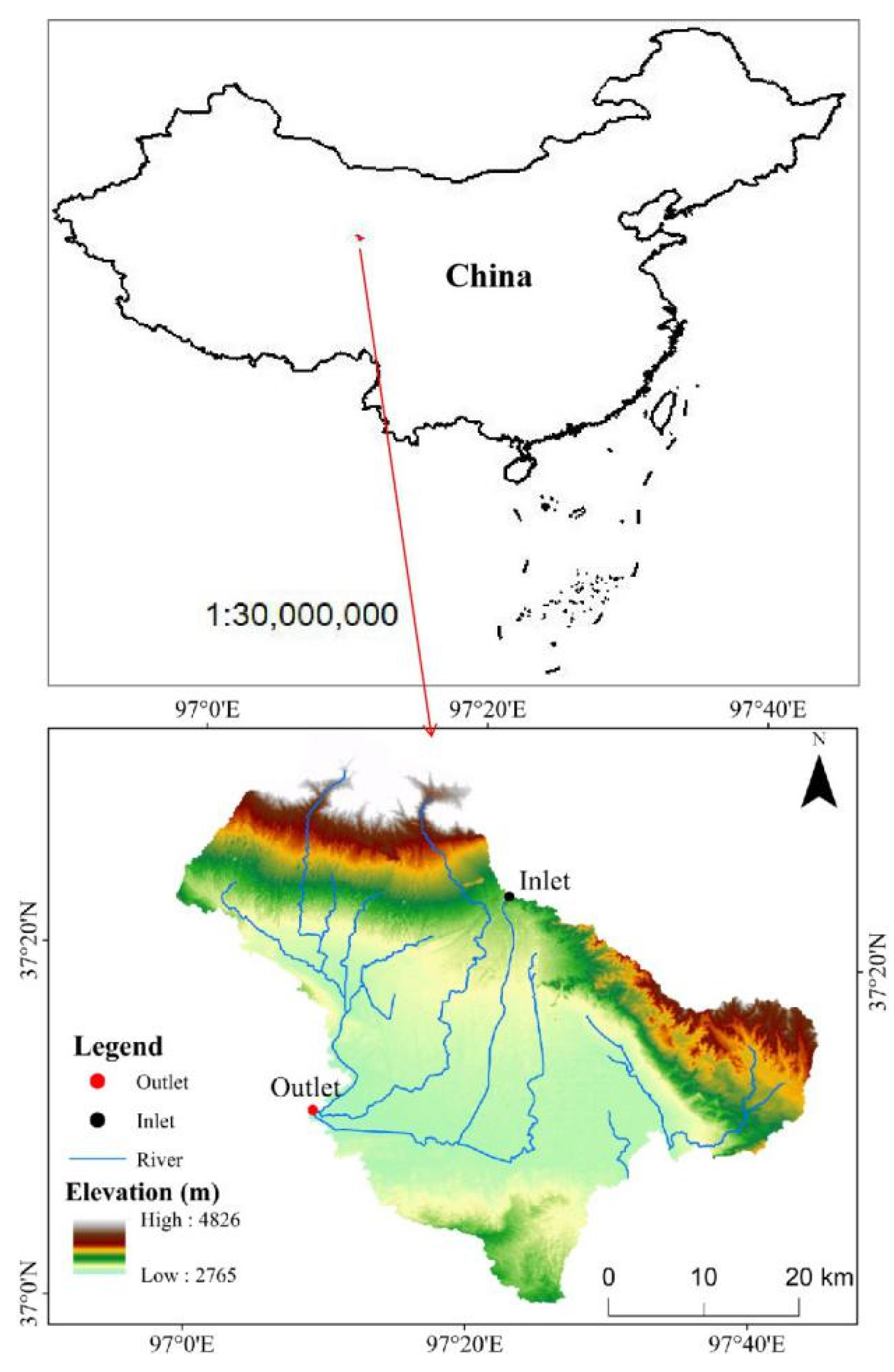
The Bayin River, which is the fourth largest river in the Qaidam Basin, is situated in the north-western region of China (Figure 1). The basin is in an arid area with annual precipitation of approximately 200 mm. The main land cover types of the area are grassland, shrubland, barren land, and farmland. The Bayin River flows out of the mountains into the middle and lower reaches, where the human population and industrial and agricultural activities are concentrated, and with frequent surface-water–groundwater exchange. The vegetation in the Bayin River basin has been restored substantially with the implementation of a series of ecological restoration measures, such as the Grain-for-Green program, over the past 20 years. However, irrigation has become essential for such artificial revegetation projects because of the arid climate and the heterogeneity in the spatial distribution of water resources.
2.2. SWAT-MODFLOW Model
In this study, the coupling of SWAT with the MODFLOW model was achieved by using the method of Bailey et al. [16]. Given the inconsistency between the two models in terms of computational spatial units, it was necessary to use a GIS platform to unify the spatial resolution before model coupling (Figure 2). First, specific spatial locations were allocated to the computational units (i.e., HRUs) of SWAT. Second, a mapping relationship was established between the HRUs of SWAT and the computational grid cells of MODFLOW on the same projected coordinate system using a GIS platform [14,15]. Third, the SWAT model was run to simulate the groundwater recharge, evaporation, and extraction with a temporal step of 1 d. Finally, the simulation results were taken as boundary conditions on the corresponding computational grid cells of MODFLOW for groundwater flow modelling [16]. The MODFLOW model was run to simulate the groundwater processes while using the groundwater monitoring data of the basin (provided by Qinghai Provincial Department of water resources) to calibrate and validate the model parameters. Meanwhile, the simulated groundwater table depth from the MODFLOW model was transferred to the computational units of surface water through the abovementioned mapping relationship to impose boundary conditions on the simulation of irrigation groundwater extraction, crop growth, and vegetation transpiration, as well as to test the simulation results [16].
2.3. SWAT-MODFLOW Model Coupled with Dynamic HRUs
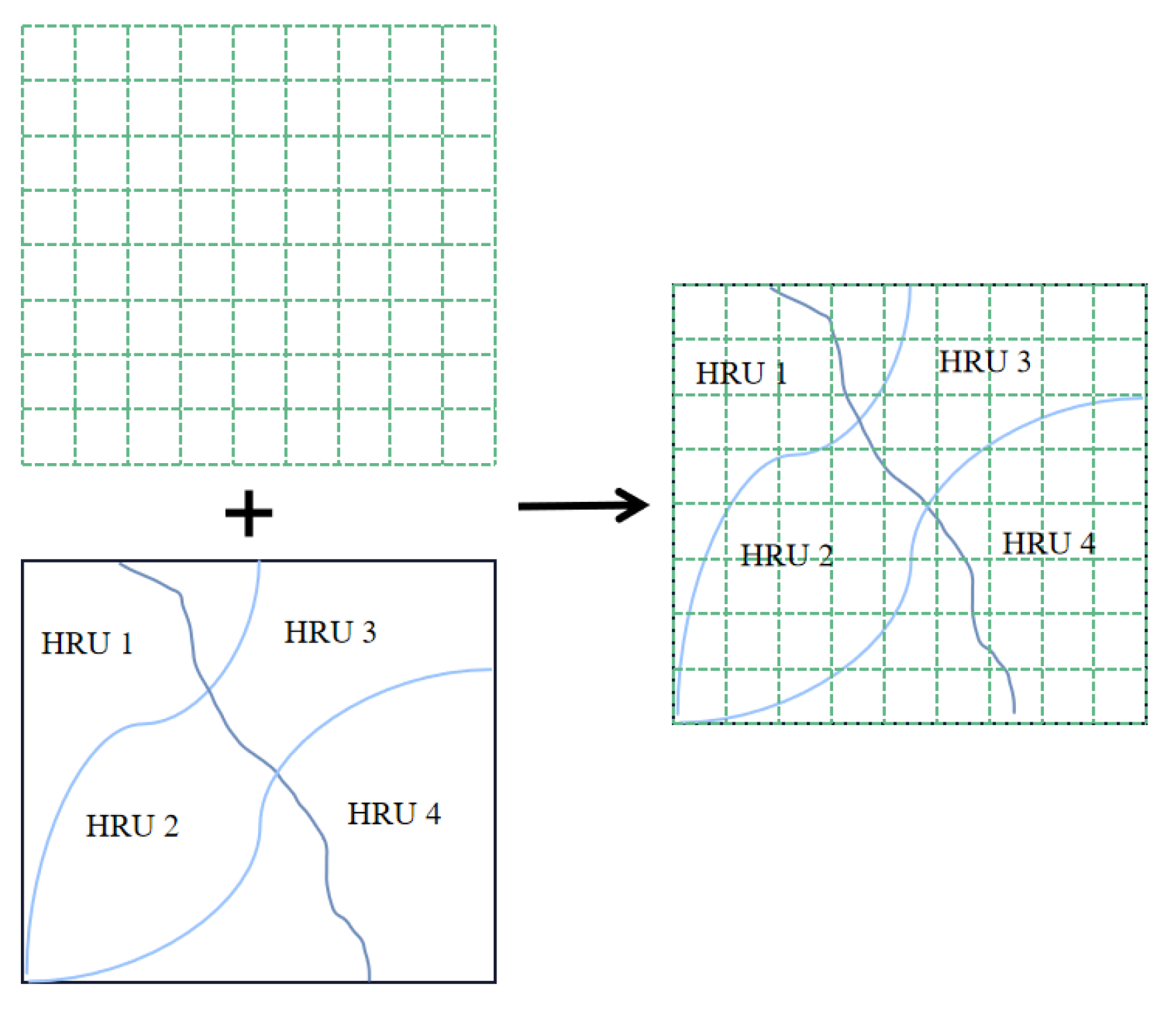
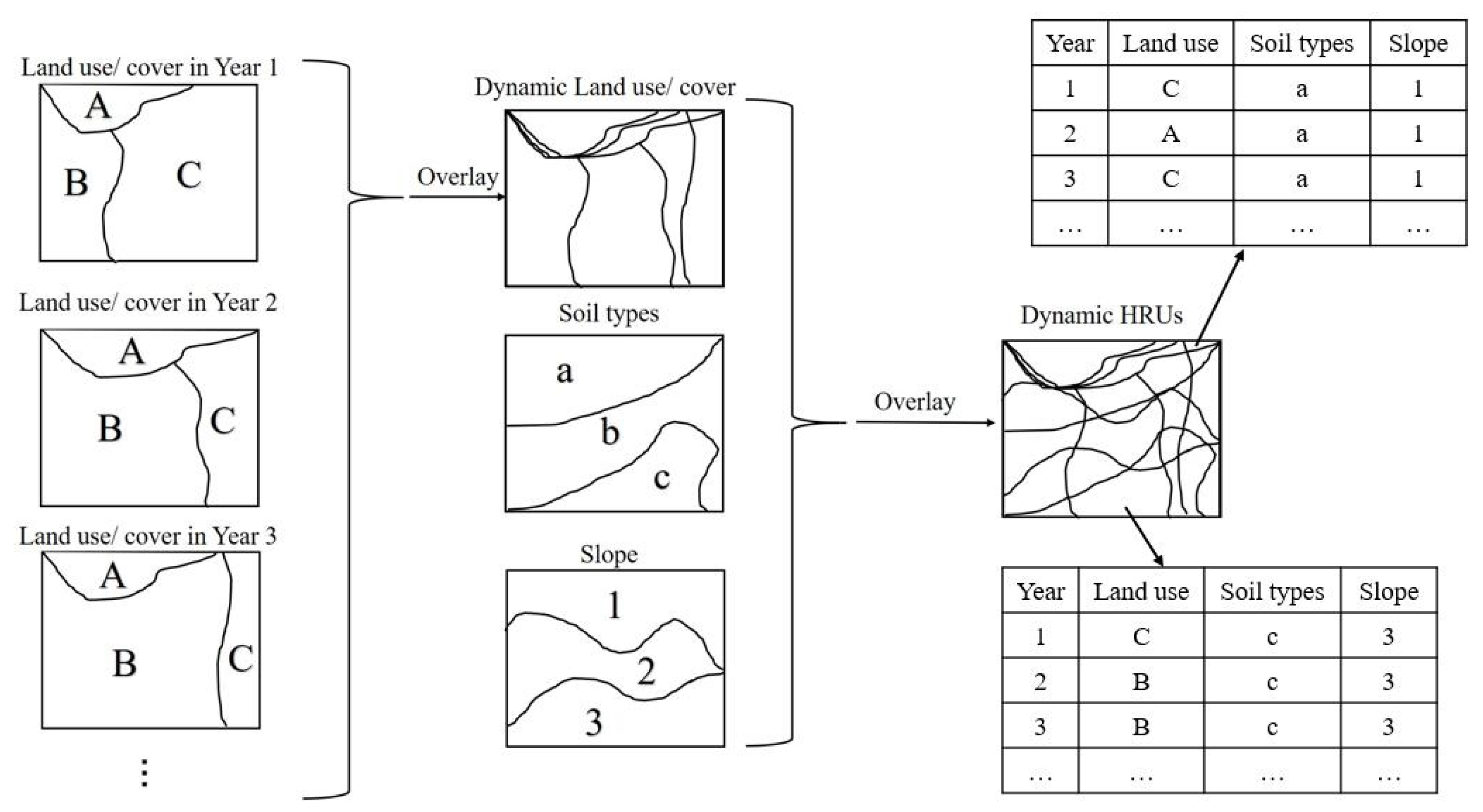
In view of the inability of the original SWAT model to effectively reflect complete or partial land cover type conversions within the same HRU, this study transformed the HRUs of the original SWAT model to dynamic HRUs to improve the original model. The generation process of dynamic HRUs is illustrated in Figure 3. In contrast to the original HRUs, the generation process of dynamic HRUs involved the defining of spatial units where there were land use/cover changes, i.e., it incorporated the concept of dynamic land use/cover. Such spatial units were combined with soil type and slope data to generate dynamic HRUs such that each had a specific and invariant location, area, and shape with variable attributes. Such dynamic HRUs can more truly reflect the land use/cover changes in the basin.
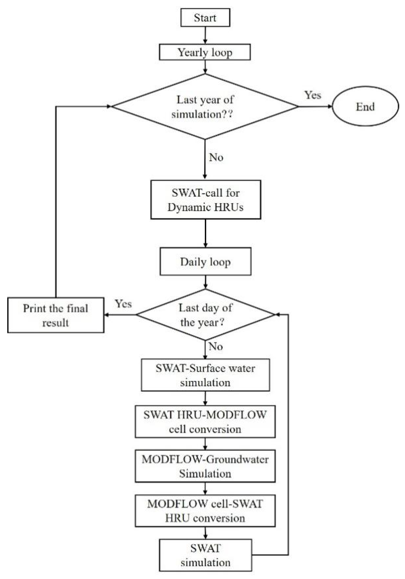
The operational flow chart of the coupled SWAT-MODFLOW model based on dynamic HRUs is shown in Figure 4. First, annual cycle simulations were performed by using corresponding HRUs (land cover). Second, daily cycle simulations were performed in which hydrological processes were simulated by SWAT. The simulation results on each HRU were mapped to the computational grid cells of MODFLOW, where these were taken as boundary conditions for groundwater flow simulations. Third, the simulated groundwater data within the grid cells were mapped to the HRUs of SWAT for subsequent SWAT computations. The above process was conducted in nested loops until the end of the simulation. Considering that the dynamic HRU-based SWAT-MODFLOW coupled model could reflect the dynamic changes in land use/cover, the model was referred to as LU-SWAT-MODFLOW.
2.4. Model Establishment
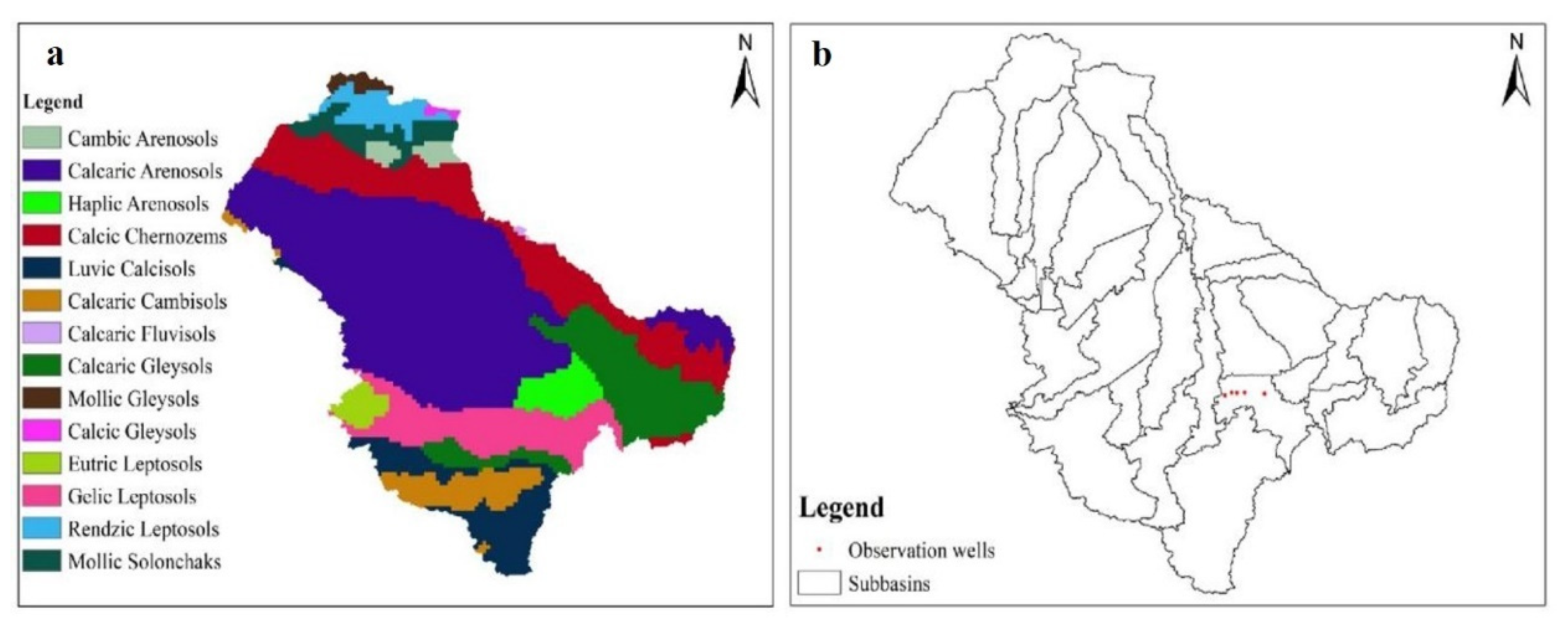
Meteorological data required for establishing the SWAT model included the daily monitoring data for precipitation, temperature, relative humidity, wind speed, and solar radiation at the Delingha weather station, which is located at the inlet shown in Figure 1. Agricultural, forestland, and grassland irrigation data were obtained from the Delingha Municipal Water Affairs Bureau (Table 1). The newest digital elevation model data (Figure 1) of 30 m resolution Shuttle Radar Topography Mission data [28] were used. Soil type data (Figure 5a) at the scale 1:1,000,000 from China were used [29], and the corresponding soil hydrological attributes were retrieved from the Qinghai Soil Record [30]. Figure 5b presents the sub-basin division map of the study region.
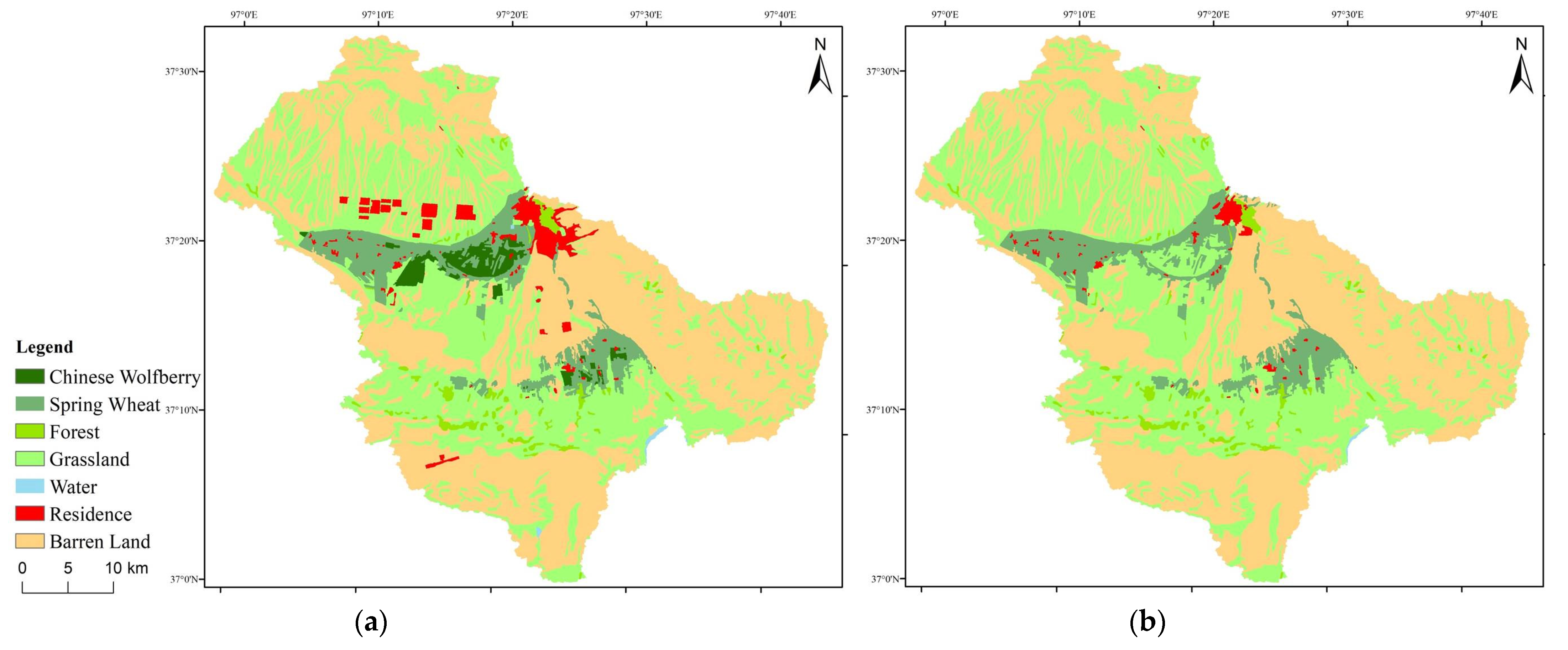
Land use type data for the simulated period (2000–2018) were derived from 30 m Landsat images. Remote sensing interpretation marks were created according to spectral features combined with field survey data and relevant geographic maps [31]. Data quality was examined by comparatively analysing field survey patches versus randomly selected patches, and the classification accuracy was determined to be over 90%. Figure 6 presents the regional spatial distribution of land use/cover in 2000 (Figure 6a) versus 2018 (Figure 6b). There were six types of land use/cover in 2000, namely, spring wheat, forest, grassland, water, residences, and barren land. There were seven types in 2018, including ‘Chinese wolfberry’ as a new type in addition to the existing six types. In the study region, Chinese wolfberry was the main tree species used for artificial revegetation. Considering the absence of Chinese wolfberry-related parameters in the built-in land use and vegetation database of SWAT, relevant initial parameters for apple trees in the SWAT model were taken as default parameters for Chinese wolfberry, and these were calibrated using the LAI data to simulate the growth process of Chinese wolfberry. Other relevant parameters of land use/cover types were either set to the default values in the built-in database of the model or obtained by calibration. Revegetation in the study region was mainly characterised by the conversion of farmland to forestland and the conversion of bare land to forestland and grassland. From 2000 to 2018, the years when evident vegetation changes (restoration) occurred in the study region were 2005, 2008, 2015, and 2018. Accordingly, the land use data for 2000, 2005, 2008, 2015, and 2018 were used to generate dynamic HRUs. In contrast, land cover types in the other years were only weakly altered and therefore ignored.
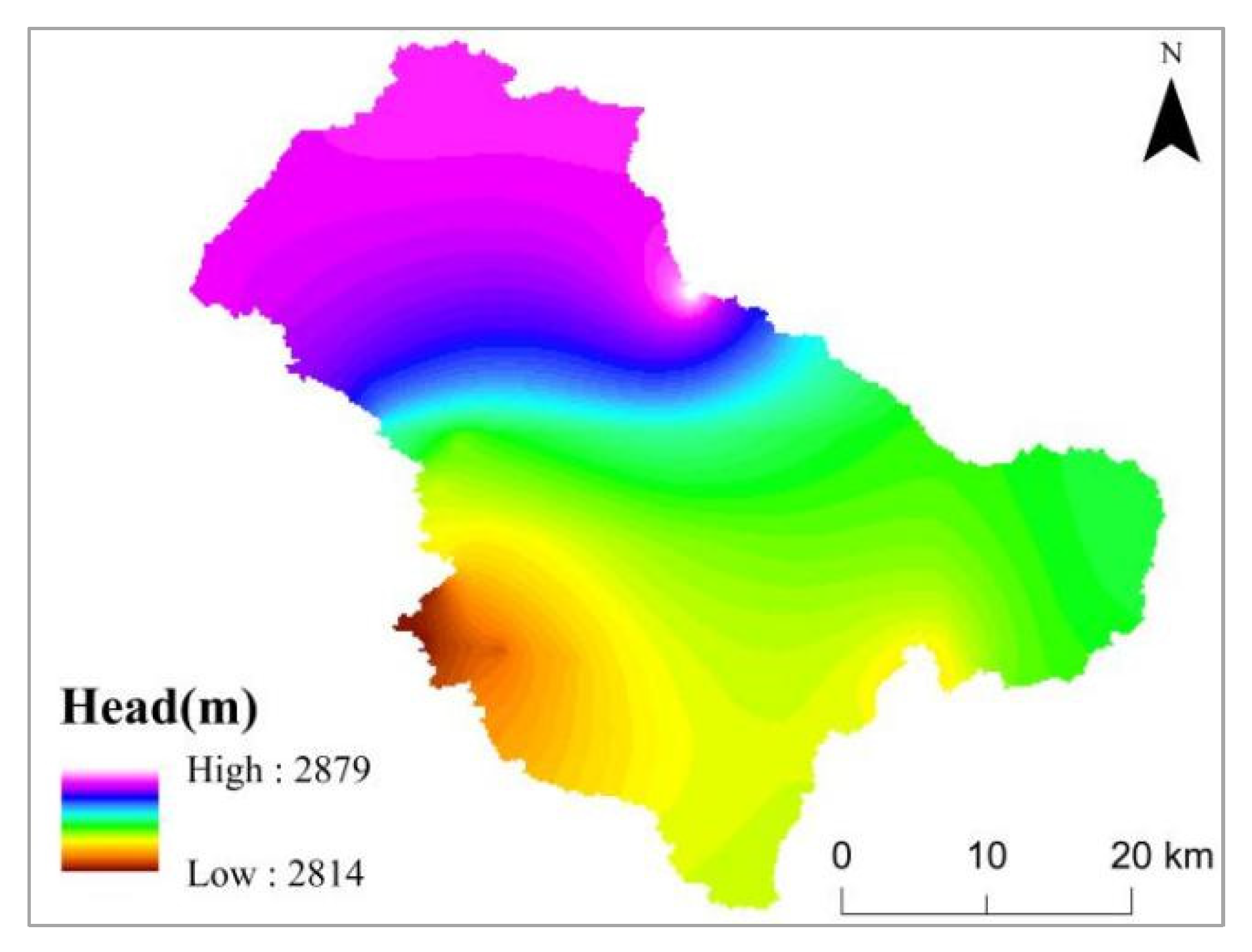
Basin boundaries delineated by the SWAT model were considered as impermeable boundaries to groundwater flow in the MODFLOW model, where the western and eastern outlets of the basin were considered as constant flow boundaries. The river network extracted by the SWAT model was considered to constitute river boundaries in the MODFLOW model. The simulated steady-state groundwater head (Figure 7) was used as the initial head for simulations of transient flow [32]. In addition, the shallow aquifers in the study region were conceptualised as being non-homogeneous and anisotropic according to relevant studies [32], and the groundwater flow was conceptualised as a two-dimensional transient flow.
2.5. Model Calibration
The years 2000–2001 were used as the model warm-up period, 2002–2011 as the model calibration period, and 2012–2018 as the model validation period. Vegetation growth parameters in the SWAT model were calibrated at HRU scales against the monthly 30 m resolution LAI data of 2002–2018 provided by the National Tibetan Plateau/Third Pole Environment Data Centre [29]. The dataset is the fusion of MODIS LAI and observed LAI in Qilian mountainous area (including the Qaidam Basin).
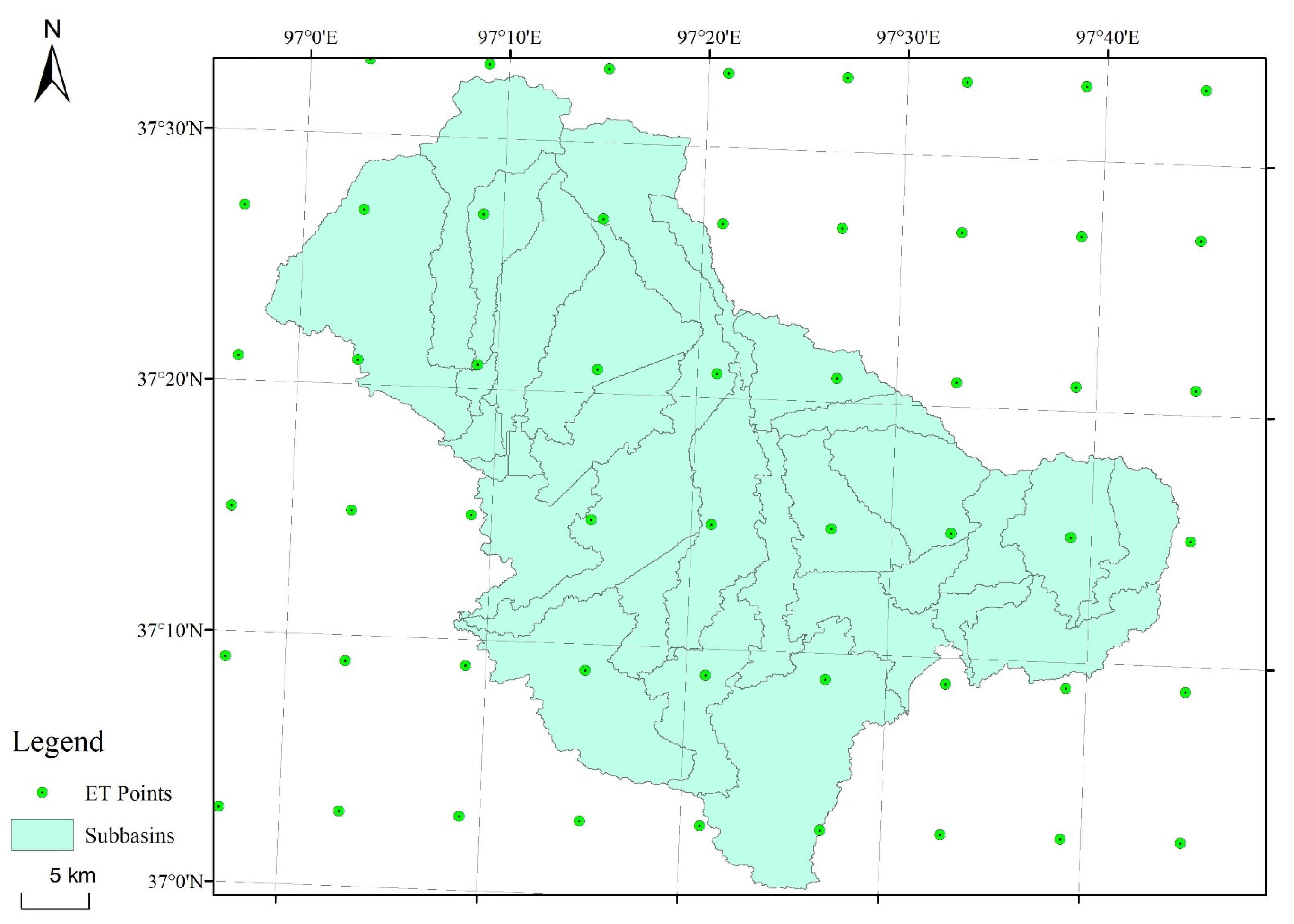
ET simulated by the LU-SWAT-MODFLOW model was calibrated at sub-basin scales against the ET data at a 0.1° × 0.1° resolution (Figure 8) provided by the National Tibetan Plateau/Third Pole Environment Data Centre [29]. The dataset is derived by employing a calibration-free nonlinear complementary relationship model with inputs of air and dew-point temperature, wind speed, precipitation, and net radiation from the China Meteorological Forcing Dataset. The dataset is validated in Northwest China and is proved to have good spatial and temporal performance [24]. Furthermore, relevant parameters (conductivity and storage) of the MODFLOW model were calibrated against monthly recorded groundwater table depth at numerous observation wells (Figure 5b) in the basin.
In this study, land cover types in the LU-SWAT-MODFLOW model varied over the years within some of the dynamic HRUs or remained invariant throughout a relatively long period within some of the HRUs. The HRUs in the latter scenario were chosen to calibrate the relevant vegetation growth parameters (Table 2) against monthly 30 m resolution LAI data [26]. The calibrated parameters were stored in a separate file, which could be visited during SWAT operations to directly tune parameters in HRUs where changes in land cover type were detected. ET-related parameter (Table 2) calibration at sub-basin scales in the present study was mainly based on the aforementioned remote sensing-derived ET data in accordance with the method of White and Chaubey [33] and Immerzeel and Droogers [25].
2.6. Model Performance Metrics
The applicability of SWAT was evaluated in terms of Nash–Sutcliffe Efficiency (NSE), percent bias (PBIAS), and squared correlation coefficient (R2). The NSE can range between −∞ and 1. If the value of the NSE was closer to 1, it was indicative of a better simulation performance and high reliability of the SWAT model. When the NSE was closer to 0.5, the model simulation results were similar to the mean of observations, that is, the model results in general were reliable. A PBIAS between −10% and 10% indicated a good simulation performance of the model. Additionally, larger values of R2 were indicative of a better simulation performance of the model. The calculation process and significance of the three metrics have been elaborated elsewhere [34]. Model performance during the simulations of the groundwater table depth was evaluated mainly in terms of the absolute error and R2 in this study.
3. Results
3.1. Regional Vegetation Change
The main types of vegetation change in the study region from 2002 to 2018 are summarised in Table 3. Specifically, the main types of vegetation change pertained to the conversion of low-coverage grassland, farmland, and bare land to forestland, in which the converted areas amounted to 2,877,518 and 321 hm2, respectively. Correspondingly, the irrigation water volume of each revegetation plot underwent dramatic changes. In addition, the conversion of farmland to forestland mainly occurred in the irrigated area of the Gahai Lake in the south-eastern part of the basin, while the conversion of low-coverage grassland and bare land to forestland mainly occurred in the irrigated area of Delingha, which is situated in the north-western part of the basin (Figure 6).
3.2. Comparison of the Original SWAT-MODFLOW and LU-SWAT-MODFLOW
3.2.1. Difference in HRUs
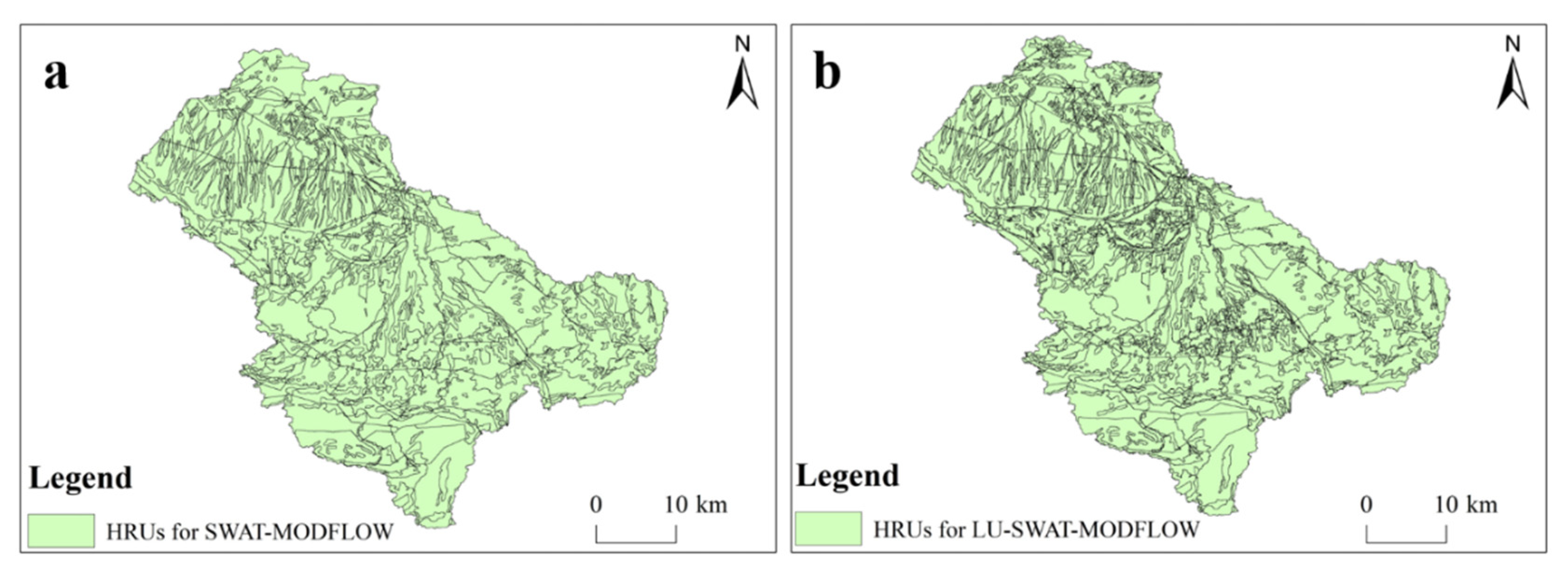
Figure 9 shows the HRUs generated by the original SWAT-MODFLOW model versus those from the LU-SWAT-MODFLOW model. The original SWAT-MODFLOW model generated 1304 HRUs, and the LU-SWAT-MODFLOW model generated 2978 HRUs. The higher number of HRUs in the new model was due to the land use/cover data of LU-SWAT-MODFLOW being a superposition of years-long data and thereby covering a higher number of patches. The higher number of HRUs also implied that the operation and parameter tuning of the LU-SWAT-MODFLOW model would be more complicated [35].
3.2.2. Comparison of the LAI Simulation Results
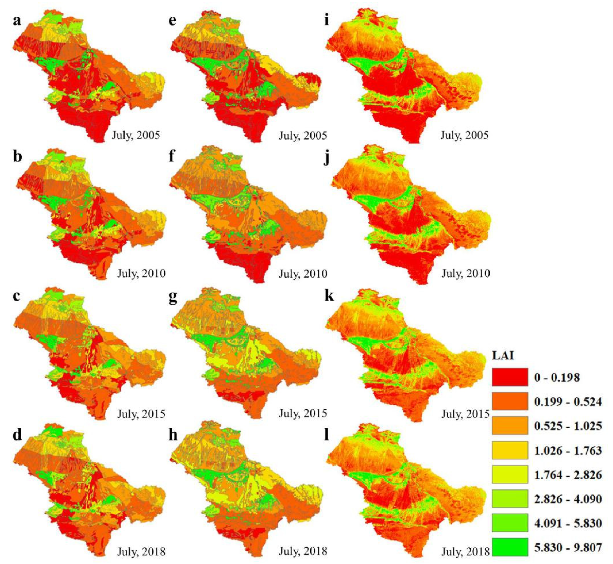
Figure 10 shows the simulated LAI from the calibrated original SWAT-MODFLOW model and the calibrated LU-SWAT-MODFLOW model for July 2005, 2010, 2015, and 2018. Compared to the remote-sensed LAI, the calibrated LU-SWAT-MODFLOW model has better performance in expressing the spatial variation of the LAI than SWAT-MODFLOW since the LU-SWAT-MODFLOW model has more HRUs. In addition, we randomly chose 10 positions in different parts of the study area and calculated the performance metrics of LAI in corresponding HRUs of original SWAT-MODFLOW and LU-SWAT-MODFLOW model, respectively. The performance metrics for the calibrated and validated original SWAT-MODFLOW model were NSE > 0.75, PBIAS of −25–25%, and R2 > 0.73, and the counterparts for the calibrated and validated LU-SWAT-MODFLOW were NSE > 0.83, PBIAS of −20–20%, and R2 > 0.83 (Table 4). This indicates that the LU-SWAT-MODFLOW model was more accurate than the original SWAT-MODFLOW model in simulations of the monthly LAI after both models were calibrated and validated.
3.2.3. Comparison of the ET Simulation Results
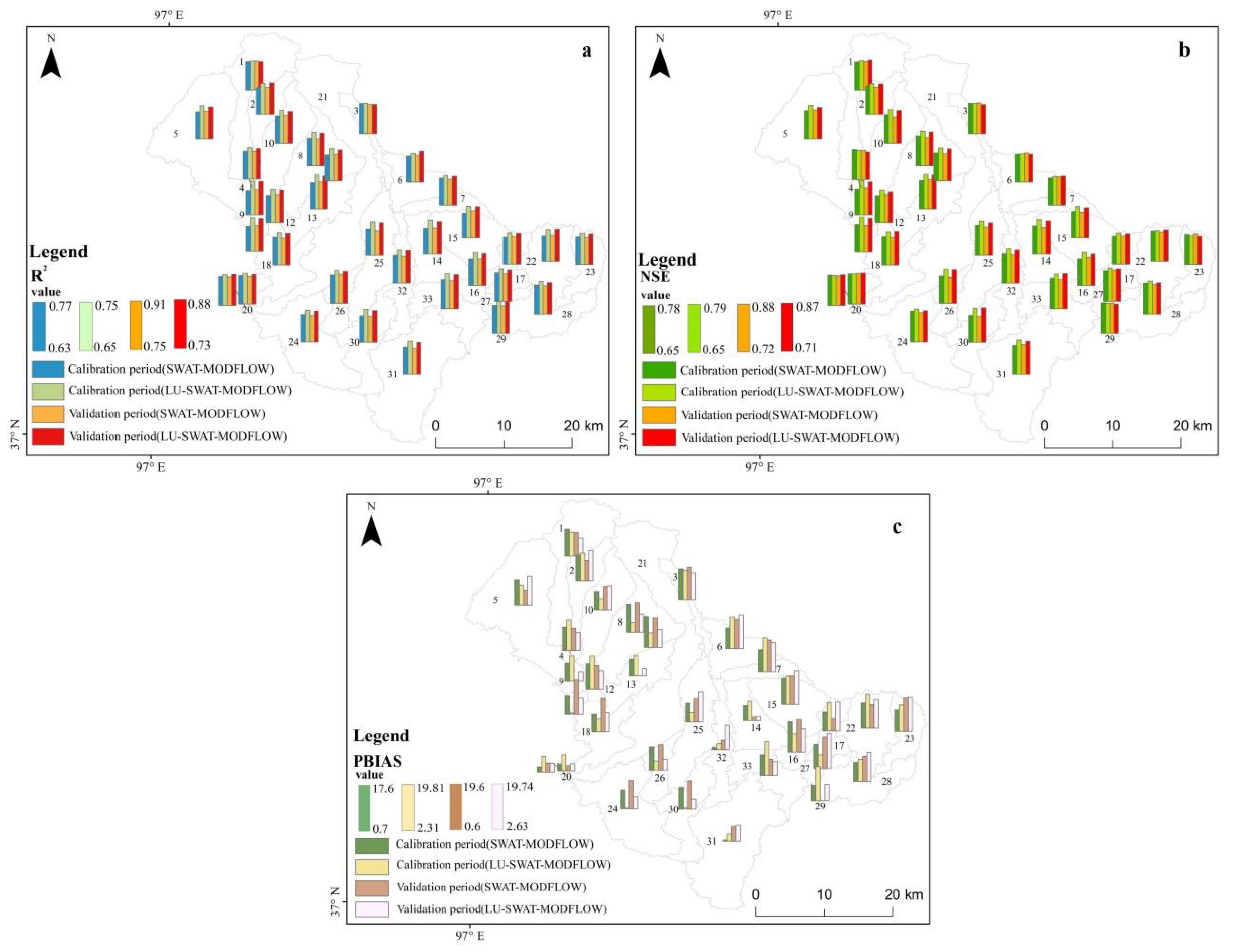
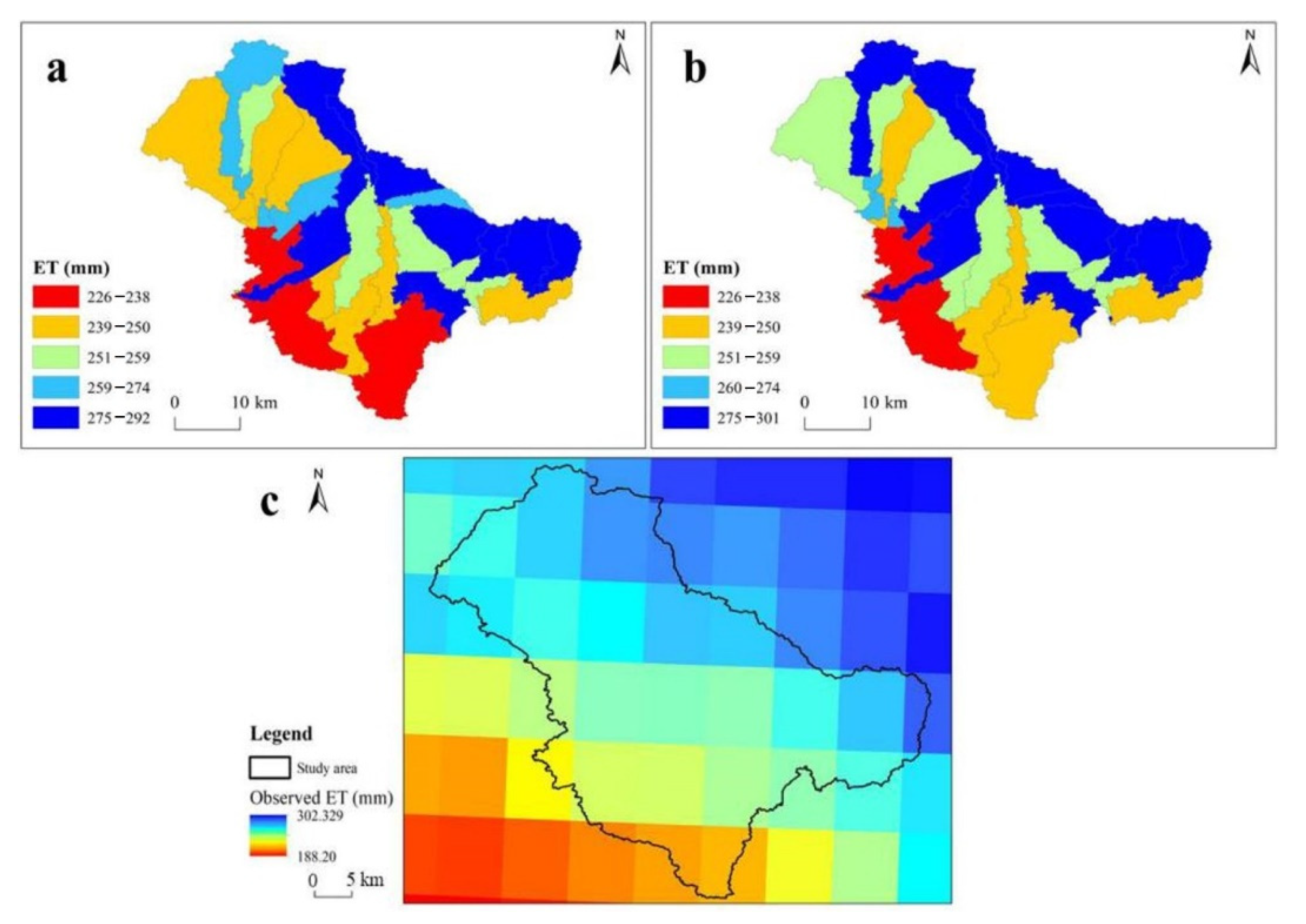
During the calibration and validation period, the performance metrics of the original SWAT-MODFLOW model were NSE > 0.65, PBIAS of −20%–20%, and R2 > 0.63 in simulations of the monthly mean ET for each sub-basin, while the counterparts for the LU-SWAT-MODFLOW model were NSE > 0.72, PBIAS of −20%–20%, and R2 > 0.73 (Figure 11). This indicates that the LU-SWAT-MODFLOW model was more accurate than the original SWAT-MODFLOW in simulations of the monthly mean ET for most of the sub-basins. Figure 12 shows the multi-year mean of the simulated ET from the original SWAT-MODFLOW model (Figure 12a) versus that of the LU-SWAT-MODFLOW model (Figure 12b) in comparison with the multi-year mean of remote sensing-derived ET (Figure 12c). The multi-year mean of remote sensing-derived ET exhibited a spatial distribution pattern of high values in the north-eastern mountains and low values in the southwestern plains, and such a distribution pattern existed for both calibrated models.
3.2.4. Comparison of the Simulation Results for Groundwater Table Depth
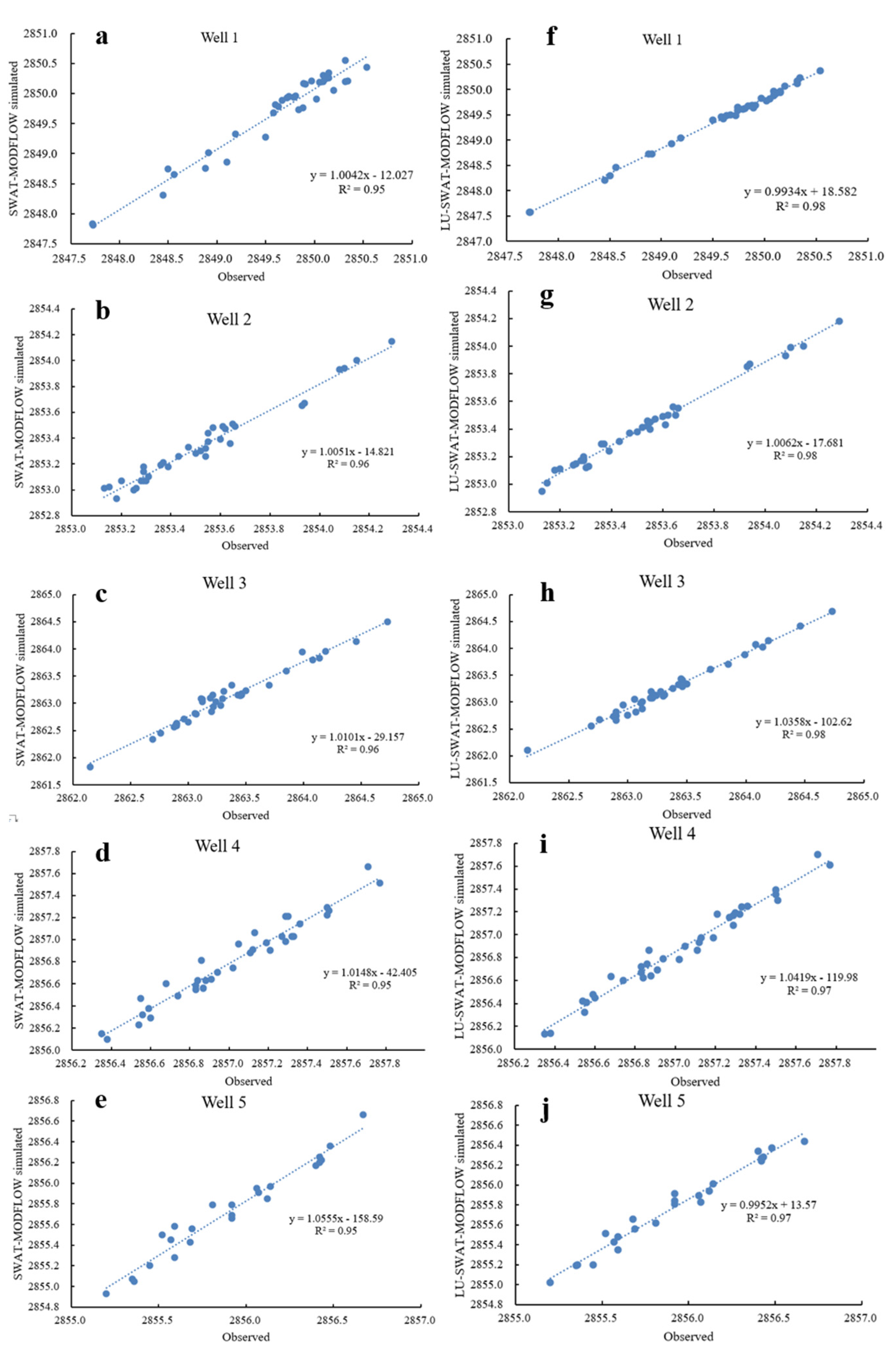
Groundwater table depth data were scarce within the study region. Observation wells 1, 2, and 3 only provided monthly data for 2009–2011, and observation well 4 only provided monthly data for 2013–2015; meanwhile, observation well 5 only provided monthly data for 2014–2015. Thus, the observed groundwater table depth of wells 1, 2, and 3 were used to calibrate the two models, and the rest were used to validate the models. Linear regression results of the simulated groundwater table depth on observed groundwater table depth were compared between the original SWAT-MODFLOW model and the LU-SWAT-MODFLOW model (Figure 13). Both models performed well in simulating the changes in the groundwater table depth of the study region, with an R2 > 0.95 and absolute error within 0.5 m. In addition, the simulation performance of LU-SWAT-MODFLOW was slightly better than that of SWAT-MODFLOW, which was likely attributed to the detailed consideration of the spatiotemporal changes in irrigation and land cover by the former model versus the latter model.
3.3. Impacts of Vegetation Change on Hydrological Processes
The case study area is located in a water consumption area of an inland river and almost never generates runoff. Thus, here we focus on the analysis of the vegetation change impacts on ET and groundwater processes.
3.3.1. Impacts on ET
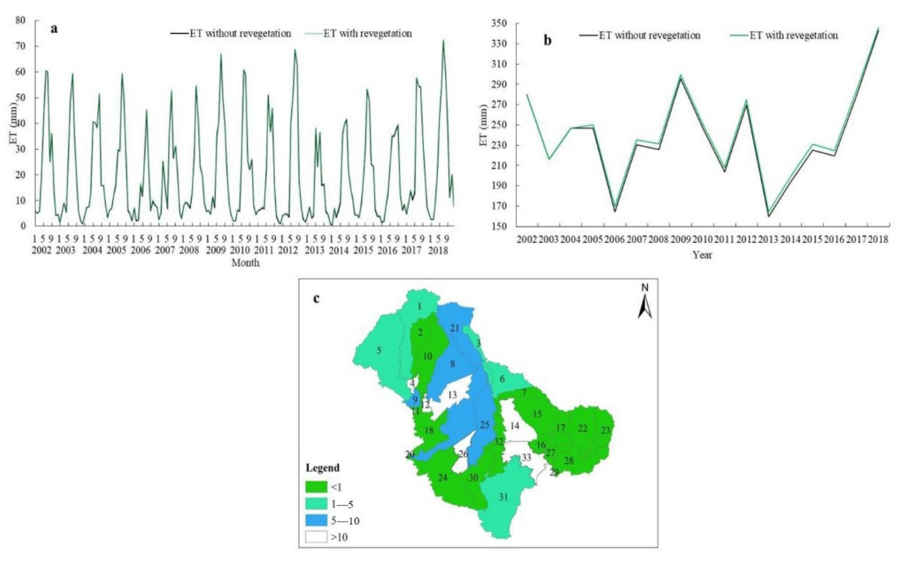
The LU-SWAT-MODFLOW model was run in the following two scenarios to accurately analyse the impacts of revegetation and the related extensive irrigation on ET: (1) revegetation was assumed absent while considering the actual changes in other types of land use/cover; and (2) the actual changes in land use/cover were considered, including those pertinent to revegetation (irrigation) and other types of land use/cover. Figure 14a shows the simulated monthly ET in the revegetation-absent scenario versus the revegetation-present scenario from 2002 to 2018. The results indicate that revegetation and related irrigation did not change the trend of monthly ET in the basin, in which the monthly ET in the revegetation-present scenario was only 1.5 mm higher than that in the revegetation-absent scenario for most months. Similarly, the trend of annual ET was almost the same in both scenarios. In 2004 and later years, ET showed weakly higher values in the revegetation-present scenario than in the revegetation-absent scenario (Figure 14b). Figure 13c illustrates the difference in the multi-year mean ET between the two scenarios in each sub-basin. Such a difference was greater than 10 mm in sub-basins 4, 12, 13, 14, 26, and 33, that is, the ET increase was most obvious in these sub-basins. Comprehensive comparisons of the land use/cover map (Figure 6) with the LAI map for the study region during the study period further confirmed that relatively obvious revegetation had been achieved in these sub-basins.
3.3.2. Impacts on Groundwater Recharge
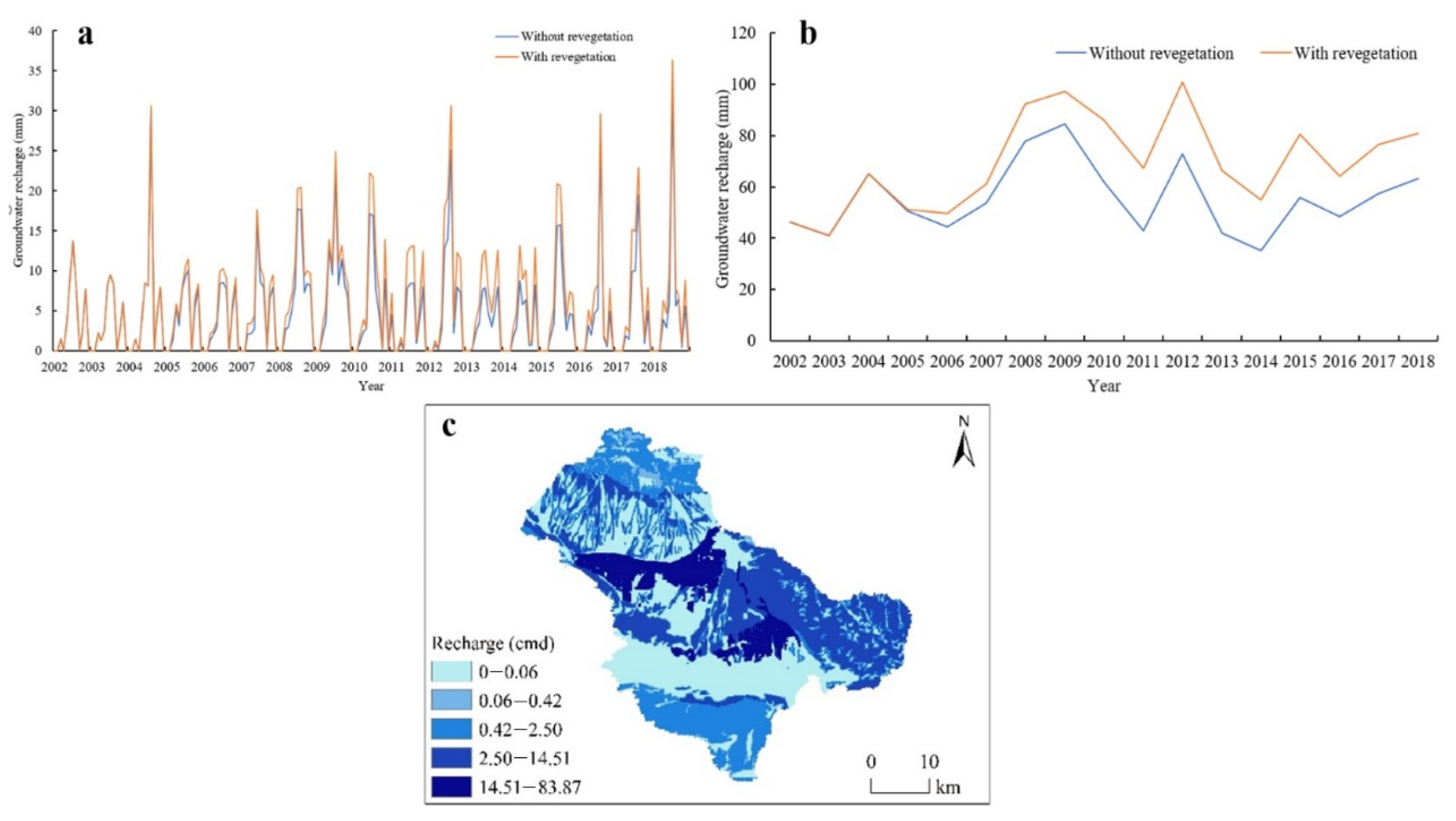
Groundwater is the most important water resource in the arid endorheic river watershed. Changes in groundwater recharge may affect the groundwater storage and further impact the ecological environment. Figure 15 shows the monthly (Figure 15a) and yearly (Figure 15b) groundwater recharge in the entire study area. After revegetation, the groundwater recharge increased by approximately 1.27 mm on average per month and 14.02 mm on average per year. Fan et al. [36], Yang and Lu [37], and Qubaja et al. [30] showed that canopy interception and root water absorption would lead to reduction of soil water, surface runoff, and groundwater recharge in woodland. However, here, although considerable areas of low-coverage grassland, farmland, and bare land were converted to forestland, the groundwater recharge with revegetation was evidently higher than that without revegetation. We reported the yearly average groundwater recharge after revegetation in the entire study area (Figure 14c). The groundwater recharge in the irrigation district where the revegetation was applied was the highest (>14.51 m3/day); that is, the irrigation for the recovered vegetation strongly affected the groundwater recharge.
3.3.3. Impacts on Surface Water and Groundwater Exchange
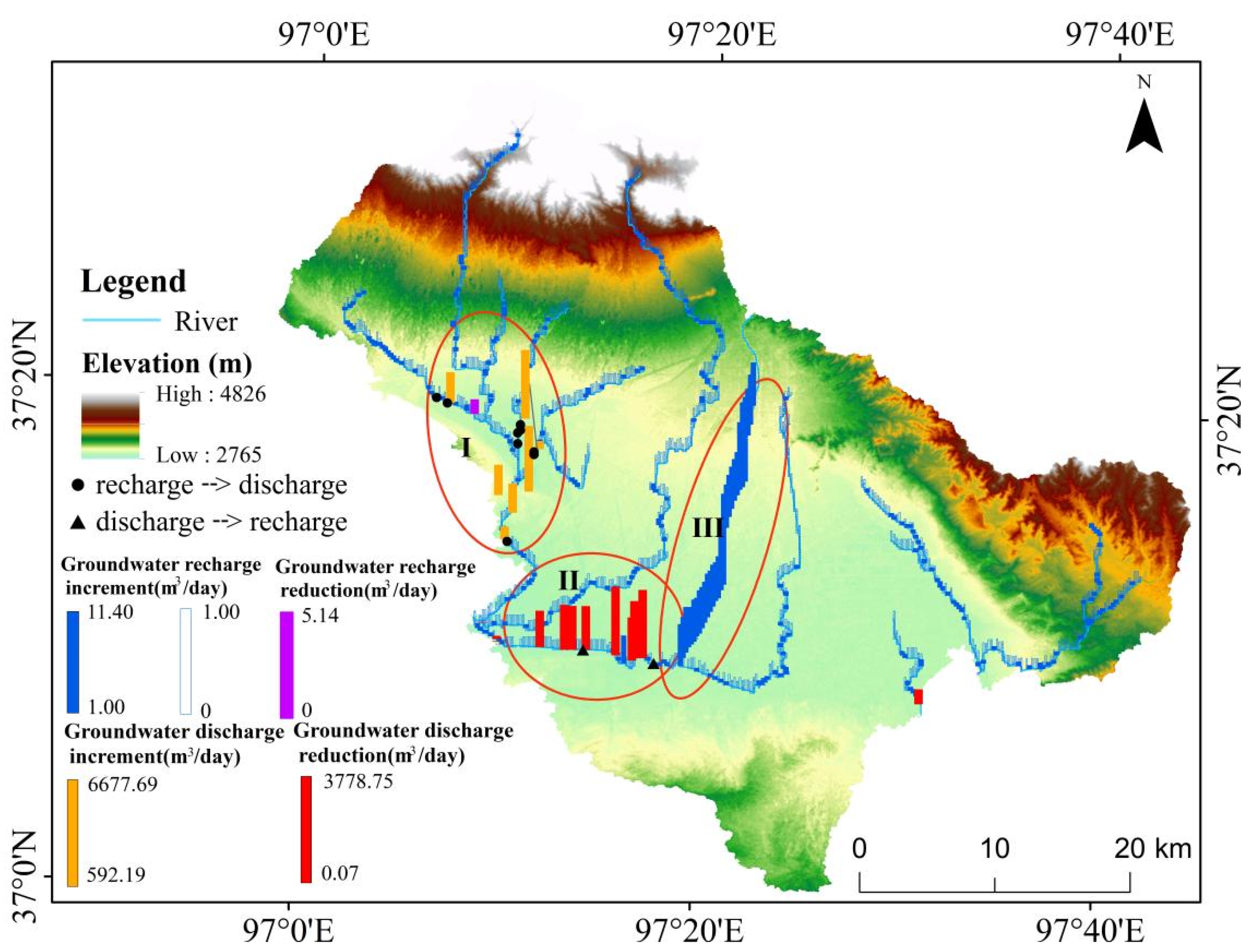
There was frequent surface-water–groundwater exchange in the study region, which dominated the regional hydrological processes. We analysed the surface water and groundwater exchange affected by revegetation. Figure 16 shows the amount of groundwater recharge and discharge in the revegetation-absent scenario minus the value in the revegetation-present scenario. Specifically, river reach I was in the upper study region, where groundwater was recharged by river water. River reach II was situated in the lower study region, where significant amounts of groundwater were discharged to the river. In river reach III, both surface water recharge to groundwater and groundwater discharge to surface water were present. River reach III was situated in the irrigated area of Delingha, where it was greatly affected by agricultural, forestland, and grassland irrigation, which led to a relatively complex pattern of surface-water–groundwater exchange. The area where river reach III was situated was also the main revegetation area of the study region. Comparisons of Figure 16 revealed that the direction of surface-water–groundwater exchange was reversed in six grid cells, which was attributed to the changes in the irrigation volume within these grid cells after revegetation.
4. Discussion
The LU-SWAT-MODFLOW model was more accurate than the original SWAT-MODFLOW model in simulating the monthly LAI after both models were calibrated and validated. LAI plays a key role in SWAT for estimating ET, canopy interception, and biomass accumulation [35]. The enhanced modelling of LAI could improve the performance of the SWAT model in eco-hydrological processes [26,38]. However, accurate simulation of LAI relies on many parameters which are difficult to calibrate. Generally, parameters of SWAT-MODFLOW are calibrated with observed data in watershed outlets or sub-basins [23,27]. Only few studies have calibrated the parameters at the HRU level because of its difficulty and complexity. In this study, the remote-sensed monthly LAI data were used to calibrate the SWAT-MODFLOW and LU-SWAT-MODFLOW at the HRU level using the SWAT-CUP software (https://swat.tamu.edu/software/swat-cup/) (accessed on 1 October 2021) with a satisfactory result. This suggests that the model calibration at the HRU level is possible and effective if the related observation data exist.
The LU-SWAT-MODFLOW model was more accurate than the original SWAT-MODFLOW in simulating the monthly mean ET for most sub-basins. Ma et al. [26] reported that canopy interception and soil water content would be seriously affected by LAI in SWAT, which would further affect ET. Therefore, the enhancements of LU-SWAT-MODFLOW in modelling the monthly ET can be attributed to the more accurate simulation of the LAI.
Revegetation projects have been conducted in both the Gahai Lake irrigated area and the irrigated area of Delingha, but the revegetation had a relatively high impact on the direction and amount of surface-water–groundwater exchange in the latter area; in the former area, there was an almost negligible impact. This discrepancy was attributed to the fact that revegetation in the Gahai Lake irrigated area was mainly characterised by the conversion of farmland to forestland, and the irrigation volume did not differ significantly between the two land cover types [38]. In contrast, the irrigated area of Delingha was dominated by the conversion of low-coverage grassland to bare land and forestland, and the former two land cover types required no irrigation, while the latter land cover type required a large irrigation volume.
This study is subjected to some limitations. On the one hand, we used land use/cover map to analyse the revegetation process in our study area. In fact, plant density, age, and growth status were not considered because of the limitations in the SWAT model. Moreover, these factors may affect the eco-hydrological processes in such an arid area [26]. On the other hand, meteorological data were scarce in both original SWAT-MODFLOW and LU-SWAT-MODFLOW models. This may impact the model performance in formulating the water budget [39,40,41]. Nonetheless, these limitations should be addressed in future studies by using and analysing different datasets.
5. Conclusions
This study was carried out in the middle and lower reaches of the Bayin River basin in the north-eastern part of the Qaidam Basin, China, where there is frequent surface-water–groundwater interaction and evident vegetation change. A LU-SWAT-MODFLOW model was developed by integrating a coupled SWAT-MODFLOW model with dynamic HRUs in view of their ability to reflect the actual land cover changes in the basin. The impacts of revegetation and related irrigation on the main hydrological processes in the basin were more accurately simulated and analysed by the LU-SWAT-MODFLOW model than by the original SWAT-MODFLOW model.
The LU-SWAT-MODFLOW model generated dynamic HRUs by pre-defining spatial units where land use/cover changes occurred during the simulated period, thereby overcoming the inability of the original SWAT model to effectively reflect the complete or partial land cover type conversion within the same HRU. This new model outperformed the original SWAT-MODFLOW model in simulating the LAI. The LAI is an important parameter of SWAT as it affects a series of processes, such as ET and infiltration; therefore, accurate simulations of the LAI are a key to accurate hydrological simulations. Moreover, the LU-SWAT-MODFLOW model outperformed the original SWAT-MODFLOW model in simulating the ET and groundwater table depth of the basin.
The LU-SWAT-MODFLOW model was run in two different scenarios, one with revegetation and the other without it, to assess the impacts of revegetation and related irrigation on the main hydrological processes in the study region. The results showed that after regional revegetation, ET in the different sub-basins increased by approximately 1.5 mm per month and by 6 mm per year. After revegetation, the groundwater recharge increased by approximately 1.27 mm on average per month and 14.02 mm on average per year. Irrigation for the recovered vegetation strongly affected the groundwater recharge. Meanwhile, the direction and amount of surface-water–groundwater exchange underwent evident changes in areas where revegetation was characterised by the conversion of low-coverage grassland and bare land to forestland. In areas where revegetation was characterised by the conversion of farmland to forestland, the irrigation volume was not greatly altered; thus, this transition had a weak impact on the direction and amount of surface-water–groundwater exchange. Changes in the direction and amount of surface-water–groundwater exchange may lead to a series of ecological and environmental issues. To avoid problems in the future, water-saving irrigation techniques should be advocated when conducting revegetation in arid inland river basins. In addition, our findings indicate that it would be advantageous to preferentially apply revegetation measures that promote the conversion of farmland to forestland/grassland provided that they do not adversely affect regional economic development.
Author Contributions
Conceptualization, X.J. and X.M.; methodology, X.J.; formal analysis, X.J.; investigation, X.J.; resources, Y.J.; data curation J.Z. and D.F.; writing—original draft preparation, X.J.; writing—review and editing, Y.J.; project administration, X.J.; funding acquisition, X.J. and X.M. All authors have read and agreed to the published version of the manuscript.
Funding
This research was funded by the National Natural Science Foundation of China, grant number 41801094 and grants from the Natural Science Foundation of Qinghai Province, China, grant number 2021-ZJ-705.
Data Availability Statement
The processed data required to reproduce these findings cannot be shared at this time as the data is also a part of an ongoing study.
Conflicts of Interest
The authors declare no conflict of interest.
References
- Feng, X.M.; Fu, B.J.; Piao, S.; Wang, S.; Ciais, P.; Zeng, Z.; Lü, Y.; Zeng, Y.; Li, Y.; Jiang, X.; et al. Revegetation in China’s Loess Plateau is approaching sustainable water resource limits. Nat. Clim. Chang. 2016, 6, 1019–1022. [Google Scholar] [CrossRef]
- Li, T.; Xia, J.; Zhang, L.; She, D.; Wang, G.; Cheng, L. An improved complementary relationship for estimating evapotranspiration attributed to climate change and revegetation in the Loess Plateau, China. J. Hydrol. 2021, 592, 125516. [Google Scholar] [CrossRef]
- Paul, M.; Rajib, A.; Negahban-Azar, M.; Shirmohammadi, A.; Srivastava, P. Improved agricultural Water management in data-scarce semi-arid watersheds: Value of integrating remotely sensed leaf area index in hydrological modelling. Sci. Total Environ. 2021, 791, 148177. [Google Scholar] [CrossRef]
- Reynolds, J.F.; Smith, D.M.S.; Lambin, E.F.; Turner, B.L., II; Mortimore, M.; Batterbury, S.P.J.; Downing, T.E.; Dowlatabadi, H.; Fernández, R.J.; Herrick, J.E.; et al. Global desertification: Building a science for dryland development. Science 2007, 316, 847–851. [Google Scholar] [CrossRef] [PubMed] [Green Version]
- Jackson, R.B.; Jobbágy, E.G.; Avissar, R.; Roy, S.B.; Barrett, D.J.; Cook, C.W.; Farley, K.A.; le Maitre, D.C.; McCarl, B.A.; Murray, B.C. Trading water for carbon with biological carbon sequestration. Science 2005, 310, 1944–1947. [Google Scholar] [CrossRef] [Green Version]
- Menz, M.H.M.; Dixon, K.W.; Hobbs, R.J. Hurdles and opportunities for landscape-scale restoration. Science 2013, 339, 526–527. [Google Scholar] [CrossRef]
- Quinn, P.; Beven, K.; Chevallier, P.; Planchon, O. The prediction of hillslope flow paths for distributed hydrological modelling using digital terrain models. Hydrol. Process 1991, 5, 59–79. [Google Scholar] [CrossRef]
- Minacapilli, M.; Iovino, M.; D’Urso, G. A distributed agro-hydrological model for irrigation water demand assessment. Agric. Water Manag. 2008, 95, 123–132. [Google Scholar] [CrossRef]
- Xu, X.; Jiang, Y.; Liu, M.; Huang, Q.; Huang, G. Modeling and assessing agro-hydrological processes and irrigation water saving in the middle Heihe River basin. Agric. Water Manag. 2019, 211, 152–164. [Google Scholar] [CrossRef]
- Arnold, J.G.; Moriasi, D.N.; Gassman, P.W.; Abbaspour, K.C.; White, M.J.; Srinivasan, R.; Santhi, C.; Harmel, R.D.; van Griensven, A.; Van Liew, M.W.; et al. SWAT: Model use, calibration, and validation. Trans. ASABE 2012, 55, 1491–1508. [Google Scholar] [CrossRef]
- Panagopoulos, Y.; Makropoulos, C.; Baltas, E.; Mimikou, M. SWAT parameterization for the identification of critical diffuse pollution source areas under data limitations. Ecol. Model. 2011, 222, 3500–3512. [Google Scholar] [CrossRef]
- Nyeko, M. Hydrologic modelling of data scarce basin with SWAT model: Capabilities and limitations. Water Resour. Manag. 2015, 29, 81–94. [Google Scholar] [CrossRef]
- Alemayehu, T.; van Griensven, A.; Bauwens, W. Evaluating CFSR and Watch data as input to SWAT for the estimation of the potential evapotranspiration in a data-scarce Eastern-African Catchment. J. Hydrol. Eng. 2016, 21, 12–18. [Google Scholar] [CrossRef]
- Yang, Q.; Zhang, X. Improving SWAT for simulating water and carbon fluxes of forest ecosystems. Sci. Total Environ. 2016, 569–570, 1478–1488. [Google Scholar] [CrossRef] [Green Version]
- Kim, N.W.; Chung, I.M.; Won, Y.S.; Arnold, J.G. Development and application of the integrated SWAT-MODFLOW model. J. Hydrol. 2008, 356, 1–16. [Google Scholar] [CrossRef]
- Bailey, R.T.; Wible, T.C.; Arabi, M.; Records, R.M.; Ditty, J. Assessing regional-scale spatio-temporal patterns of groundwater-surface water interactions using a coupled SWAT-MODFLOW model. Hydrol. Process 2016, 30, 4420–4433. [Google Scholar] [CrossRef]
- Jin, X.; He, C.; Zhang, L.; Zhang, B. A modified groundwater module in SWAT for improved streamflow simulation in a large, arid endorheic river watershed in Northwest China. Chin. Geogr. Sci. 2018, 28, 47–60. [Google Scholar] [CrossRef] [Green Version]
- Liu, W.; Park, S.; Bailey, R.T.; Molina-Navarro, E.; Andersen, H.E.; Thodsen, H.; Nielsen, A.; Jeppesen, E.; Jensen, J.S.; Jensen, J.B.; et al. Comparing SWAT with SWAT-MODFLOW hydrological simulations when assessing the impacts of groundwater abstractions for irrigation and drinking water. Hydrol. Earth Syst. Sci. 2019. [Google Scholar] [CrossRef] [Green Version]
- Semiromi, M.T.; Koch, M. Analysis of spatio-temporal variability of surface–groundwater interactions in the Gharehsoo river basin, Iran, using a coupled SWAT-MODFLOW model. Environ. Earth Sci. 2019, 78, 1–21. [Google Scholar] [CrossRef]
- Mosase, E.; Ahiablame, L.; Park, S.; Bailey, R. Modelling potential groundwater recharge in the Limpopo River Basin with SWAT-MODFLOW. Groundw. Sustain. Dev. 2019, 9, 100260. [Google Scholar] [CrossRef]
- Jafari, F.; Kiem, A.S.; Javadi, S.; Nakamura, T.; Nishida, K. Fully integrated numerical simulation of surface water-groundwater interactions using SWAT-MODFLOW with an improved calibration tool. J. Hydrol. 2021, 35, 100822. [Google Scholar] [CrossRef]
- Zhang, C.; Shoemaker, C.A.; Woodbury, J.D.; Cao, M.; Zhu, X. Impact of human activities on stream flow in the Biliu River basin, China. Hydrol. Process 2013, 27, 2509–2523. [Google Scholar] [CrossRef]
- Wang, Q.; Liu, R.; Men, C.; Guo, L.; Miao, Y. Effects of dynamic land use inputs on improvement of SWAT model performance and uncertainty analysis of outputs. J. Hydrol. 2018, 563, 874–886. [Google Scholar] [CrossRef]
- Ma, N.; Szilagyi, J.; Zhang, Y.; Liu, W. Complementary-relationship-based modeling of terrestrial evapotranspiration across China during 1982–2012: Validations and spatiotemporal analyses. J. Geophys. Res. Atmos. 2019, 124, 4326–4351. [Google Scholar] [CrossRef]
- Immerzeel, W.W.; Droogers, P. Calibration of a distributed hydrological model based on satellite evapotranspiration. J. Hydrol. 2008, 349, 411–424. [Google Scholar] [CrossRef]
- Ma, T.; Duan, Z.; Li, R.; Song, X. Enhancing SWAT with remotely sensed LAI for improved modelling of ecohydrological process in subtropics. J. Hydrol. 2019, 570, 802–815. [Google Scholar] [CrossRef] [Green Version]
- Jin, X.; Jin, Y.X. Calibration of a distributed hydrological model in a data-scarce basin based on GLEAM datasets. Water 2020, 12, 897. [Google Scholar] [CrossRef] [Green Version]
- 30 m Resolution Shuttle Radar Topography Mission Data. Available online: http://gdex.cr.usgs.gov/gdex/ (accessed on 1 October 2021).
- Available online: https://data.tpdc.ac.cn/ (accessed on 1 October 2021).
- Qubaja, R.; Amer, M.; Tatarinov, F.; Rotenberg, E. Partitioning evapotranspiration and its long-term evolution in a dry pine forest using measurement-based estimates of soil evaporation. Agric. For. Meteorol. 2019, 281, 107831. [Google Scholar] [CrossRef]
- Liu, J.; Liu, M.; Zhuang, D.; Zhang, A.; Deng, X. Study on spatial pattern of land-use change in China during 1995–2000. Sci. China Earth Sci. 2003, 46, 373–384. [Google Scholar] [CrossRef]
- Yang, N.; Zhou, P.; Wang, G.; Zhang, B.; Shi, Z.; Liao, F.; Li, B.; Chen, X.; Guo, L.; Dang, X.; et al. Hydrochemical and isotopic interpretation of interactions between surface water and groundwater in Delingha, Northwest China. J. Hydrol. 2021, 126243. [Google Scholar] [CrossRef]
- White, K.L.; Chaubey, I. Sensitivity analysis, calibration, and validations for a multisite and multivariable SWAT model. J. Am. Water Resour. Assoc. 2005, 41, 1077–1089. [Google Scholar] [CrossRef]
- Moriasi, D.N.; Arnold, J.G.; Van Liew, M.W.; Bingner, R.L.; Harmel, R.D.; Veith, T.L. Model evaluation guidelines for systematic quantification of accuracy in watershed simulations. Trans. ASABE 2007, 50, 885–900. [Google Scholar] [CrossRef]
- Alemayehu, T.; Griensven, A.; Woldegiorgis, B.T.; Bauwens, W. An improved SWAT vegetation growth module and its evaluation for four tropical ecosystems. Hydrol. Earth Syst. Sci. 2017, 21, 4449–4467. [Google Scholar] [CrossRef] [Green Version]
- Fan, J.; Oestergaard, K.T.; Guyot, A.; Lockington, D.A. Estimating groundwater recharge and evapotranspiration from water table fluctuations under three vegetation covers in a coastal sandy aquifer of subtropical Australia. J. Hydrol. 2014, 519, 1120–1129. [Google Scholar] [CrossRef] [Green Version]
- Yang, K.; Lu, C. Evaluation of land-use change effects on runoff and soil erosion of a hilly basin—The Yanhe River in the Chinese Loess Plateau. Land Degrad. Dev. 2018, 29, 1211–1221. [Google Scholar] [CrossRef]
- Samimi, M.; Mirchi, A.; Moriasi, D.; Ahn, S.; Alian, S.; Taghvaeian, S.; Sheng, Z. Modeling arid/semi-arid irrigated agricultural watersheds with SWAT: Applications, challenges, and solution strategies. J. Hydrol. 2020, 125418. [Google Scholar] [CrossRef]
- Earls, J.; Dixon, B. A Comparison of SWAT Model-Predicted Potential Evapotranspiration Using Real and Modelled Meteorological Data. Vadose Zone J. 2008, 7, 570–580. [Google Scholar] [CrossRef]
- Ji, L.; Duan, K. What is the main driving force of hydrological cycle variations in the semiarid and semi-humid Weihe River Basin, China? Sci. Total Environ. 2019, 684, 254–264. [Google Scholar] [CrossRef]
- Li, D.C.; Zhao, X.; Zhang, G.L. Chinese Earth Series—Qinghai Volume [M]; Science Press: Beijing, China, 2019. (In Chinese) [Google Scholar]
Figure 1.
Study area.

Figure 2.
Integration of Soil and Water Assessment Tool (SWAT) and MODFLOW computing units.

Figure 3.
Production of dynamic hydrological response units (HRUs).

Figure 4.
Flowchart of the SWAT-MODFLOW coupled model based on dynamic HRUs.

Figure 5.
(a) Soil types in the study area and (b) sub-basins input to the SWAT model.

Figure 6.
Revegetation status of the study region in (a) 2000 and (b) 2018.

Figure 7.
Initial groundwater head for MODFLOW.

Figure 8.
Locations of ET data points.

Figure 9.
HRUs generated by (a) SWAT-MODFLOW and (b) LU-SWAT-MODFLOW.

Figure 10.
Simulated leaf area index (LAI) from the (a–d) calibrated original SWAT-MODFLOW model, (e–h) calibrated LU-SWAT-MODFLOW model, and (i–l) remote-sensed LAI.
Figure 10.
Simulated leaf area index (LAI) from the (a–d) calibrated original SWAT-MODFLOW model, (e–h) calibrated LU-SWAT-MODFLOW model, and (i–l) remote-sensed LAI.

Figure 11.
NSE (a), R2 (b), PBIAS (c) of the calibrated original SWAT-MODFLOW model versus the calibrated LU-SWAT-MODFLOW model in simulating evapotranspiration in each sub-basin.
Figure 11.
NSE (a), R2 (b), PBIAS (c) of the calibrated original SWAT-MODFLOW model versus the calibrated LU-SWAT-MODFLOW model in simulating evapotranspiration in each sub-basin.

Figure 12.
Multi-year mean ET simulated by (a) SWAT-MODFLOW, (b) LU-SWAT-MODFLOW, and (c) retrieved from remote sensing images.
Figure 12.
Multi-year mean ET simulated by (a) SWAT-MODFLOW, (b) LU-SWAT-MODFLOW, and (c) retrieved from remote sensing images.

Figure 13.
Monthly groundwater table depth simulated by the (a–e) SWAT-MODFLOW model versus the (f–j) LU-SWAT-MODFLOW model.
Figure 13.
Monthly groundwater table depth simulated by the (a–e) SWAT-MODFLOW model versus the (f–j) LU-SWAT-MODFLOW model.

Figure 14.
(a) Monthly and (b) yearly ET with revegetation and without revegetation; (c) yearly average ET change in different sub-basins after revegetation.
Figure 14.
(a) Monthly and (b) yearly ET with revegetation and without revegetation; (c) yearly average ET change in different sub-basins after revegetation.

Figure 15.
(a) Monthly and (b) yearly groundwater recharge with and without revegetation; (c) yearly average groundwater recharge after revegetation in space.
Figure 15.
(a) Monthly and (b) yearly groundwater recharge with and without revegetation; (c) yearly average groundwater recharge after revegetation in space.

Figure 16.
Revegetation impacts on groundwater recharge and discharge.


Table 1.
Irrigation volume in the study region.
| Irrigation Type | Annual Irrigation Rate (m3/hm2) | Number of Times of Irrigation | Irrigation Duration |
|---|---|---|---|
| Agricultural irrigation | 5800 | 6 | March–October |
| Forest irrigation | 5400 | 6 | April–November |
| Grassland irrigation | 3600 | 5 | April–November |
Table 2.
Vegetation growth and ET-related parameters in SWAT.
| Processes | Parameter | Description |
|---|---|---|
| Vegetation growth-related parameters | BLAI | Maximum potential leaf area index |
| LAIMX_1 | Fraction of the maximum leaf area index corresponding to the 1st point on the optimal leaf area development curve | |
| FRGRW1 | Fraction of the plant growing season corresponding to the 1st point on the optimal leaf area development curve | |
| LAIMX_2 | Fraction of the maximum leaf area index corresponding to the 2nd point on the optimal leaf area development curve | |
| FRGRW2 | Fraction of the plant growing season corresponding to the 2nd point on the optimal leaf area development curve | |
| DLAI | Fraction of growing season when leaf area begins to decline | |
| BIO_E | Radiation use efficiency | |
| EXT_COEF | Light extinction coefficient | |
| GSI | Maximum canopy stomatal conductance | |
| HVSTI | Harvest index for the optimal growing condition | |
| T-BASE | Minimum (base) temperature for plant growth | |
| ET-related parameters | SOL_AWC | Available water content |
| RFINC | Monthly rainfall increment | |
| GWREVAP | Groundwater revap coefficient | |
| BLAI | Maximum potential leaf area index | |
| ESCO | Soil evaporation compensation factor | |
| EPCO | Plant uptake compensation factor |
Table 3.
Main types of revegetation in the study region.
| Main Type of Revegetation | Revegetation Area (hm 2) | Change in the Annual Irrigation Rate (m3/hm2·a) |
|---|---|---|
| Conversion of low-coverage grassland to forestland | 2877 | 0→5400 |
| Conversion of farmland to forestland | 518 | 5800→5400 |
| Conversion of bare land to forestland | 321 | 0→5400 |
Table 4.
Performance of the original SWAT-MODFLOW model versus the LU-SWAT-MODFLOW model in simulating LAI.
Table 4.
Performance of the original SWAT-MODFLOW model versus the LU-SWAT-MODFLOW model in simulating LAI.
| HRU | SWAT-MODFLOW | LU-SWAT-MODFLOW | ||||||||||
|---|---|---|---|---|---|---|---|---|---|---|---|---|
| Calibration Period | Validation Period | Calibration Period | Validation Period | |||||||||
| NSE | PBIAS | R2 | NSE | PBIAS | R2 | NSE | PBIAS | R2 | NSE | PBIAS | R2 | |
| E1 | 0.85 | 20.84 | 0.83 | 0.81 | 17.63 | 0.79 | 0.92 | 14.11 | 0.88 | 0.87 | 16.54 | 0.85 |
| E2 | 0.86 | 23.71 | 0.85 | 0.80 | 21.25 | 0.76 | 0.91 | 11.13 | 0.87 | 0.86 | 14.52 | 0.83 |
| W1 | 0.82 | 19.89 | 0.82 | 0.78 | 15.65 | 0.75 | 0.88 | 13.45 | 0.90 | 0.84 | 17.89 | 0.88 |
| W2 | 0.83 | 17.41 | 0.81 | 0.75 | 19.32 | 0.73 | 0.89 | 12.65 | 0.89 | 0.83 | 19.21 | 0.84 |
| S1 | 0.85 | 13.72 | 0.84 | 0.81 | 17.29 | 0.77 | 0.90 | 10.99 | 0.90 | 0.86 | 16.54 | 0.86 |
| S2 | 0.83 | 19.24 | 0.81 | 0.79 | 14.23 | 0.78 | 0.91 | 11.11 | 0.90 | 0.85 | 17.32 | 0.87 |
| N1 | 0.87 | 15.36 | 0.85 | 0.77 | 13.22 | 0.78 | 0.93 | 14.65 | 0.92 | 0.88 | 15.21 | 0.89 |
| N2 | 0.86 | 17.52 | 0.84 | 0.76 | 11.21 | 0.77 | 0.90 | 17.53 | 0.89 | 0.84 | 18.56 | 0.90 |
| C1 | 0.84 | 21.49 | 0.83 | 0.78 | 22.17 | 0.76 | 0.92 | 16.46 | 0.90 | 0.87 | 14.12 | 0.87 |
| C2 | 0.85 | 20.76 | 0.83 | 0.81 | 19.78 | 0.74 | 0.91 | 13.02 | 0.92 | 0.83 | 11.76 | 0.89 |
Publisher’s Note: MDPI stays neutral with regard to jurisdictional claims in published maps and institutional affiliations. |
© 2021 by the authors. Licensee MDPI, Basel, Switzerland. This article is an open access article distributed under the terms and conditions of the Creative Commons Attribution (CC BY) license (https://creativecommons.org/licenses/by/4.0/).
Share and Cite
MDPI and ACS Style
Jin, X.; Jin, Y.; Mao, X.; Zhai, J.; Fu, D. Modelling the Impact of Vegetation Change on Hydrological Processes in Bayin River Basin, Northwest China. Water 2021, 13, 2787. https://0-doi-org.brum.beds.ac.uk/10.3390/w13192787
AMA Style
Jin X, Jin Y, Mao X, Zhai J, Fu D. Modelling the Impact of Vegetation Change on Hydrological Processes in Bayin River Basin, Northwest China. Water. 2021; 13(19):2787. https://0-doi-org.brum.beds.ac.uk/10.3390/w13192787
Chicago/Turabian StyleJin, Xin, Yanxiang Jin, Xufeng Mao, Jingya Zhai, and Di Fu. 2021. "Modelling the Impact of Vegetation Change on Hydrological Processes in Bayin River Basin, Northwest China" Water 13, no. 19: 2787. https://0-doi-org.brum.beds.ac.uk/10.3390/w13192787
Note that from the first issue of 2016, this journal uses article numbers instead of page numbers. See further details here.