Prediction of Total Nitrogen and Phosphorus in Surface Water by Deep Learning Methods Based on Multi-Scale Feature Extraction

Abstract

To improve the precision of water quality forecasting, the variational mode decomposition (VMD) method was used to denoise the total nitrogen (TN) and total phosphorus (TP) time series and obtained several high- and low-frequency components at four online surface water quality monitoring stations in Poyang Lake. For each of the aforementioned high-frequency components, a long short-term memory (LSTM) network was introduced to achieve excellent prediction results. Meanwhile, a novel metaheuristic optimization algorithm, called the chaos sparrow search algorithm (CSSA), was implemented to compute the optimal hyperparameters for the LSTM model. For each low-frequency component with periodic changes, the multiple linear regression model (MLR) was adopted for rapid and effective prediction. Finally, a novel combined water quality prediction model based on VMD-CSSA-LSTM-MLR (VCLM) was proposed and compared with nine prediction models. Results indicated that (1), for the three standalone models, LSTM performed best in terms of mean absolute error (MAE), mean absolute percentage error (MAPE), and the root mean square error (RMSE), as well as the Nash–Sutcliffe efficiency coefficient (NSE) and Kling–Gupta efficiency (KGE). (2) Compared with the standalone model, the decomposition and prediction of TN and TP into relatively stable sub-sequences can evidently improve the performance of the model. (3) Compared with CEEMDAN, VMD can extract the multiscale period and nonlinear information of the time series better. The experimental results proved that the averages of MAE, MAPE, RMSE, NSE, and KGE predicted by the VCLM model for TN are 0.1272, 8.09%, 0.1541, 0.9194, and 0.8862, respectively; those predicted by the VCLM model for TP are 0.0048, 10.83%, 0.0062, 0.9238, and 0.8914, respectively. The comprehensive performance of the model shows that the proposed hybrid VCLM model can be recommended as a promising model for online water quality prediction and comprehensive water environment management in lake systems.

1. Introduction

The main sources of fresh water supply for domestic water, industrial water, and agricultural water use are rivers, lakes, and groundwater, respectively. However, in many areas, fresh water resources are often limited, and the optimal management of water resources should consider quality and quantity [1]. Among them, water quality monitoring is of great importance for the quality of water resource optimization management. Water quality monitoring refers to the process of collecting, measuring, and analyzing water samples to understand the physical, chemical, and biological conditions of the water body. The complexity of the detection methods and procedures for different water quality parameters depends on the characteristics of the water body, such as total nitrogen (TN) and total phosphorus (TP), which usually require intensive testing processes of sampling, laboratory processing, and result analysis. However, some other parameters, such as the potential of hydrogen (PH), turbidity (TUB), electrical conductivity (EC), and dissolved oxygen (DO), can be easily measured onsite using sensors [2].

TN and TP are the main nutrients that lead to the eutrophication of water bodies [3,4,5,6]. To assess the trophic level of lakes, TN and TP should be tested routinely. Common measurement methods include colorimetry, manual distillation, and ion chromatography. However, the complexity of the biophysical and chemical processes in lake water renders the detection of TN and TP difficult [7,8,9]. One common challenge is that nutrient tests should be performed as soon as the sample is collected because as the sample sits longer, the organisms that live in the water will consume nutrients and the nutrient concentrations in the water sample will be modified. Another challenge is that the determination of TN and TP requires the measurement of various forms of nitrogen and phosphorus separately, and the results of all the different forms under each group must be combined to determine TN and TP. These procedures and steps are difficult and time consuming [10].

To save time, materials, and labor costs in monitoring water quality, many scholars have attempted to use predictive models to replace monitoring water quality and have achieved satisfactory results. Currently, the models that have been proposed for water quality prediction are mainly divided into deterministic and uncertain water quality models [11]. Among them, the deterministic water quality model is a process-based numerical simulation model, and the soil and water assessment tool (SWAT) [12] and storm water management model [13] have been widely used to predict surface water quality. For example, Lin et al. [14] applied the SWAT model to the Xiekengxi River watershed in Lin’an City, Zhejiang Province, China. The runoff, sediment, TN, and TP of the basin were predicted, and the sensitivities of SWAT to digital elevation models of different resolutions were analyzed. Baek et al. [15] improved the low-impact development module of the SWMM model and accurately simulated the total suspended solids, chemical oxygen demand, TN, and TP in Korean urban watersheds.

Although these traditional process-based deterministic models can accurately simulate water quality, they usually require a large amount of input data, such as hydrological and water quality parameters, which greatly increases the computational cost. In addition, in some complex watersheds, the input data and parameters of some of these processes are not available [1,10]. These problems greatly limit the scope of application of deterministic water quality models. Therefore, the use of uncertainty mathematical models for water quality prediction has gradually become the focus of research [16,17,18,19]. Moreover, with the rapid development of machine learning and neural networks in recent years, data-driven uncertainty water quality prediction models based on machine learning and neural networks, such as random forest [20,21], support vector regression (SVR) [22,23], least squares support vector regression [24,25], extreme learning machine (ELM) [26,27], adaptive neurofuzzy inference system [28,29], backpropagation (BP) neural network [30,31], and neural network radial basis function [32,33], have been widely used.

However, these water quality prediction models based on machine learning and neural networks face problems. Due to the “shallow” learning mechanism of these models, their ability to address input features and capture the long-term correlation of time series is very limited [34]. As a result, they have poor performance in predicting time series with nonlinear and non-stationary characteristics, especially the time series of water quality parameters affected by different natural and human factors. In response to this problem, many researchers have turned their attention to LSTMs [35] that have nonlinear predictive capabilities, faster convergence speed, and the ability to capture the long-term correlation of time series [34]. Compared with other models mentioned above, LSTM shows better stability and higher accuracy [36,37,38], thereby providing ideas for further research on water quality prediction. However, it remains challenging to accurately forecast non-linear and non-stationary features together only using standalone AI-based models.

The hybrid model is receiving increasing attention from researchers. The hybrid model maintains the advantages of multiple models through an effective combination. Commonly used combination methods include data preprocessing and parameter selection and optimization [39]. For highly nonlinear and nonstationary time series, the decomposition method is an effective data-preprocessing method. For example, some common decomposition methods include wavelet decomposition [11,40], empirical mode decomposition (EMD) [41], ensemble empirical mode decomposition (EEMD) [42], complete ensemble empirical mode decomposition with adaptive noise (CEEMDAN) [11,37], and VMD) [43]. At the same time, some hybrid models based on decomposition methods and intelligent optimization algorithms can also be used. For instance, Song et al. [44] used VMD to decompose the original DO time series into multiple sub-sequences and then utilized the LSSVM model optimized by the sparrow search algorithm (SSA) to predict the sub-sequences and proposed a VMD-SSA-LSSVM hybrid water quality prediction model that is applied to the Yangtze River Basin in China. Here, VMD-SSA-LSSVM was demonstrated as an effective method for predicting non-stationary and non-linear water quality parameter series. Huang et al. [45] proposed an interval prediction method of deep auto-regression recurrent neural network based on VMD and SSA using actual water quality data to simulate and verify the effectiveness of the model. The results show that VMD-DeepAR-SSA is significant compared with existing methods, and it improved the quality and performance of interval predictions.

Notably, some researchers opted to use different machine learning methods for predictive modeling according to the different fluctuation trends of subsequences. For example, Li et al. [18] used EEMD to decompose DO into multiple components and reconstruct them into four terms, namely, high-frequency term, intermediate-frequency term, low-frequency term, and trend term. Among them, high- and intermediate-frequency terms are predicted by LSSVM, the low-frequency term is predicted by the BP neural network with an optimal mind evolutionary computation, and the trend term is predicted by the grey model. This research demonstrated that the use of appropriate machine learning and neural network methods for the components of different fluctuation trends can improve the performance of the hybrid model more effectively. In addition, some researchers have proposed the two-layer decomposition hybrid prediction model. Fijani et al. [46] used the CEEMDAN method to decompose the chlorophyll-a and DO time series into multiple sub-sequences. The VMD method is used to further decompose the intrinsic mode function (IMF) with the highest frequency. The subsequences of each stage are modeled by ELM, and the hybrid model has remarkable performance and robustness on relatively complex real-time data sets. Dong and Zhang [47] applied the standalone model, single-layer decomposition hybrid model, and two-layer decomposition hybrid model to predict the polycyclic aromatic hydrocarbons in water, and the CEEMDAN-VMD-LSTM hybrid prediction model had the best performance.

Although the above hybrid forecasting models show excellent results, the decomposition-based forecasting models suffer from some common shortcomings. In these studies, the entire time series was decomposed into multiple IMFs, and then each IMF was divided into calibration set and validation set, the models were built separately, and finally, the prediction results of each IMF were summed and reconstructed into prediction results. In this situation, some future information that is unknown at the present moment is used in the modeling system, which thus does not represent the actual conditions.

This study aims to explore the optimal combined prediction model by comparing and investigating different decomposition methods, as well as different traditional machine learning algorithms. It also proposes improvements for the problem of SSA, which is used to calibrate the hyperparameters of machine learning models. Moreover, a new method for dividing data is proposed to solve the problem that future information is used in the modeling process. Finally, this paper developed a new hybrid water quality prediction model called VMD-CSSA-LSTM-MLR (VCLM) for highly nonlinear and non-stationary water quality parameter time series.

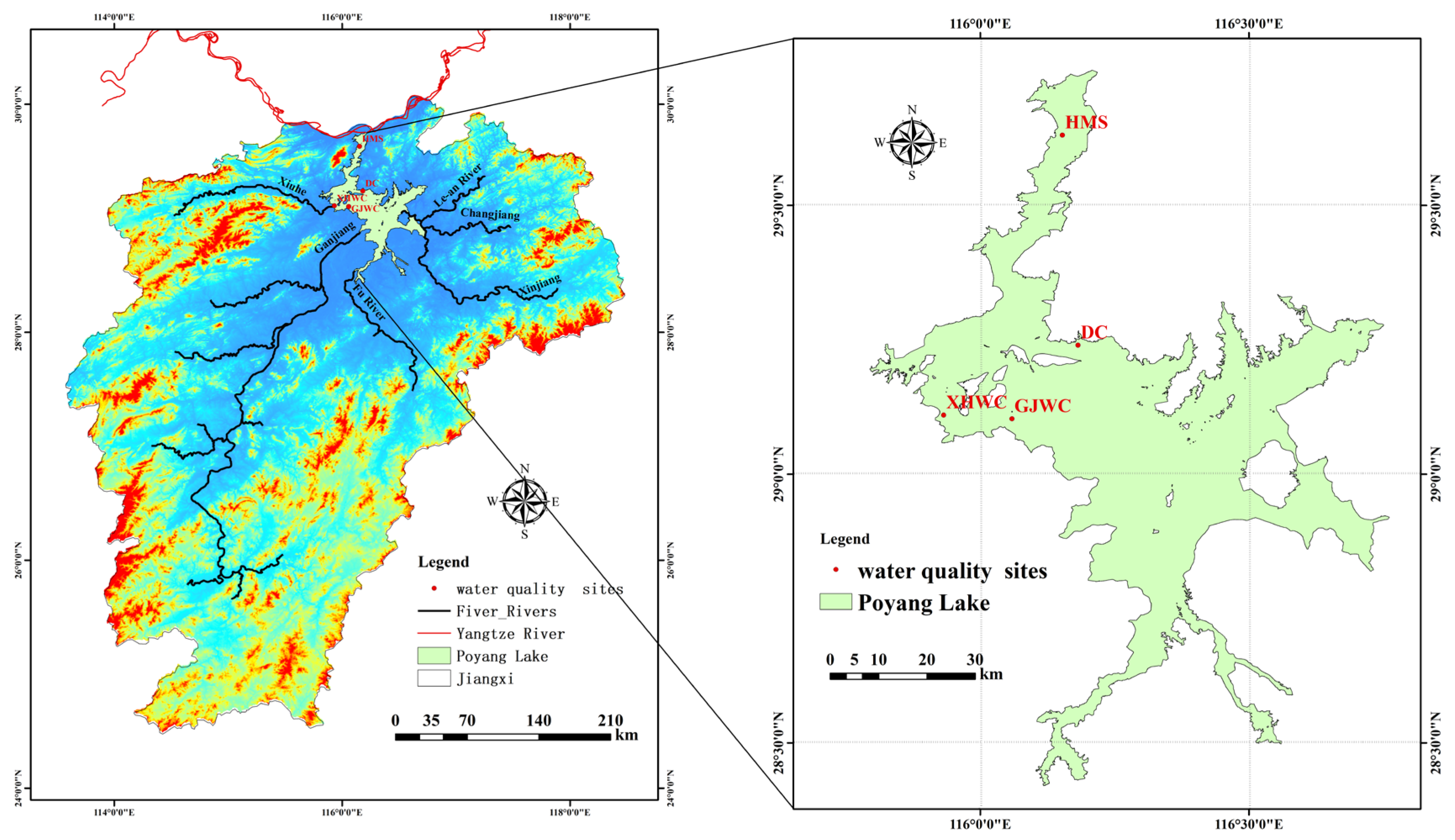
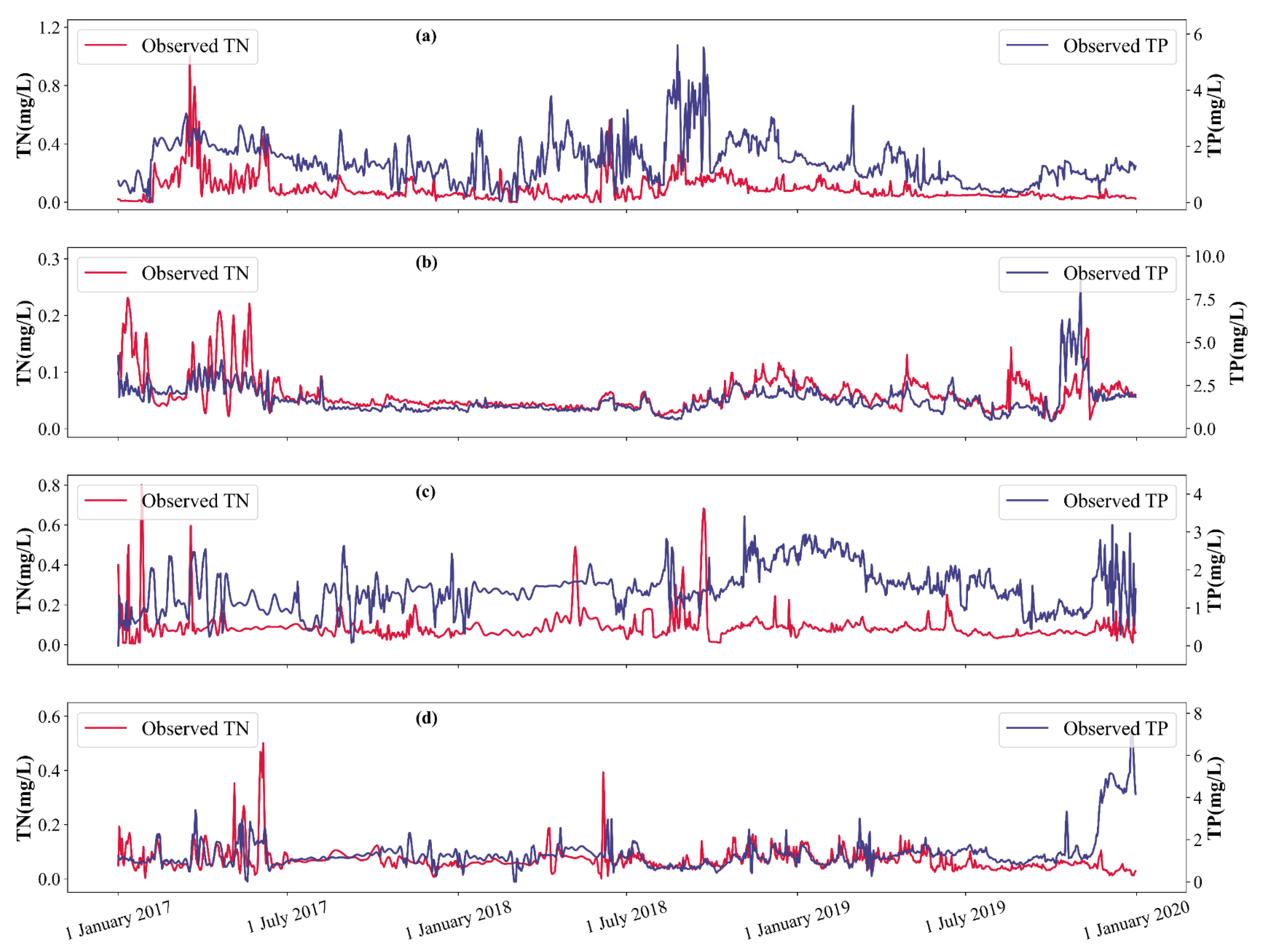
2. Study Area and Data

Poyang Lake is the largest fresh-water lake in China. It is located in the northern part of Jiangxi Province and on the south bank of the Yangtze River (115°49′–116°46′ E, 28°24′–29°46′ N). With Songmen Mountain as the boundary, the lake area is divided into north and south. The main lake area in the south is wide, and the waterway into the river in the north is relatively long and narrow. The total area of the river basin is 162,000 km², which represents 9% of the total area of the Yangtze River basin. The average annual runoff is 149.1 billion cubic meters, and it flows into the Yangtze River at the mouth of the lake. The average annual water that enters the Yangtze River represents approximately 15.6% of the total water volume of the Yangtze River. The annual variation of the average water level in the lake area is 9.59–15.36 m.

Since the 1970s–1980s, China has carried out water quality monitoring for water resources. Poyang Lake is the largest freshwater lake in China. According to the estimation of Li et al. [48], the TN load of Poyang Lake is 92,111 t/a, and the TP load is 13,599 t/a. The nutrient load of the five tributaries of the lake is the main source, accounting for more than 65% of the total load. According to Tang et al. [49], the construction land in Poyang Lake area has also been expanding year by year since 1995, which will directly or indirectly lead to more nutrient load in Poyang Lake. Wantzen et al. [50] also pointed out that hydrological characteristics also play an important role in the transport and transfer of pollutants in the lake. In recent years, with the influence of global climate change and human activities, especially with the establishment of Three Gorges Dam, the hydrological characteristics of Poyang Lake area have changed significantly. The change of flow of Yangtze River caused by the storage of Three Gorges Reservoir leads to the weakening of the river force on the lake, which makes more water from the lake flow into Yangtze River from July to March. Under this series of effects, it is crucial to establish a water quality prediction model that meets current needs in response to the current trend of new hydrological characteristics.

The water level changes drastically during the year. It is a typical seasonal lake. Figure 1 shows the study area. In this study, several typical sites in Poyang Lake, such as Duchang (DC) Station, Hamashi (HMS) Station, Ganjiang Wucheng (GJWC) Station, and Xiuhe Wucheng (XHWC) Station of the Poyang Lake, were selected as cases to implement the proposed model.

The data studied in this paper are derived from the daily monitoring data of the four online surface water quality monitoring stations mentioned above from 1 January 2017 to 1 January 2020 (1096 observations in total). The TN and TP data of the four online surface water quality monitoring stations of DC, HMS, GJWC, and XHWC are shown in Figure 2. In addition to TN and TP data, dissolved oxygen (DO), electric conductivity (EC), turbidity (TUB), total ammonia nitrogen (TAN), potential of hydrogen (PH), water temperature (WTMP), precipitation (PRCP), and water level (WL) data were also included.

3. Methodology

3.1. VMD

3.1.1. Theory of VMD

The VMD algorithm is a novel decomposition method, which is based on a variational problem constructed by Wiener filtering and Hilbert transform [51]. The original signal is decomposed into finite bandwidth intrinsic mode functions (IMFs), and the center frequency of each IMF is extracted to ensure that the mode fluctuates with the center frequency. VMD is composed of two parts: constructing the variational problem and solving the variational problem, where the variational problem can be written as follows:

$$\left\{\begin{array}{c}\underset{\left\{u_k\right\}\left\{{\omega }_k\right\}}{min}\left\{{\displaystyle \sum _{k=1}^K{‖{\partial }_t\left[\left(\delta \left(t\right)+\frac{j}{\pi t}\right)\times u_k\left(t\right)\right]e^{-j{\omega }_{k}t}‖}_2^2}\right\}\\ s.t.{\displaystyle \sum _{k=1}^K{u}_k}=f\end{array}\right.$$

(1)

where $u_k$ denotes the k-th IMF, ${\omega }_k$ denotes the center frequency of the k-th IMF, and $f$ denotes the original signal. The introduction of penalty factor $\alpha$ and Lagrange multipliers $\lambda (t)$ allows the conversion of the constrained variational problem into an unconstrained variational problem, which is denoted as follows.

$$\begin{array}{l}L\left(\left\{u_k\right\},\left\{{\omega }_k\right\},\lambda \right)=\alpha {\displaystyle \sum _{k=1}^K{‖{\partial }_t\left[\left(\delta \left(t\right)+\frac{j}{\pi t}\right)\times u_k\left(t\right)\right]e^{-j\omega kt}‖}_2^2}\\ \begin{array}{cc}& \end{array}+{‖f\left(t\right)-{\displaystyle \sum _{k=1}^K{u}_k\left(t\right)}‖}_2^2+〈\lambda \left(t\right),f\left(t\right)-{\displaystyle \sum _{k=1}^K{u}_k\left(t\right)}〉\end{array}$$

(2)

The alternating multiplication method is used to solve the non-constrained variational problem, namely, the minimum point of the extended Lagrange expression can be obtained by alternating and updating $u_k$, ${\omega }_k$, and $\lambda$. $u_k$, ${\omega }_k$, and $\lambda$ are expressed as follows.

$$\left\{\begin{array}{l}{\widehat{u}}_k^{n+1}\left(\omega \right)=\frac{\widehat{f}\left(\omega \right)-{\displaystyle \sum _{i<k}^K{\widehat{u}}_i^{n+1}}(\omega )-{\displaystyle \sum _{i>k}^K{\widehat{u}}_i^n}(\omega )+\frac{\widehat{\lambda }\left(\omega \right)}{2}}{1+2\alpha {\left(\omega -{\omega }_k^n\right)}^2}\\ {\widehat{\omega }}_k^{n+1}=\frac{{\displaystyle {\int }_0^{\infty }\omega }{\left|{\widehat{u}}_k^{n+1}\left(\omega \right)\right|}^{2}d\omega }{{\displaystyle {\int }_0^{\infty }{\left|{\widehat{u}}_k^{n+1}\left(\omega \right)\right|}^{2}d\omega }}\\ \\ {\widehat{\lambda }}^{n+1}(\omega )={\widehat{\lambda }}^n(\omega )+\tau (\widehat{f}(\omega )-{\displaystyle \sum _{k=1}^K{\widehat{u}}_k^{n+1}(\omega ))}\end{array}\right.$$

(3)

VMD divides the frequency band based on the characteristics of the original signal, and continuously updates the IMF and its center frequency using the above formula, and the update stops when the constraints are satisfied, finally realizing the adaptive decomposition of the original signal.

3.1.2. Determination of the Level of Decomposition

To determine the value of $K$ adaptively, this paper adopts permutation entropy (PE) optimization algorithm [52,53]. The principle of the algorithm is to calculate the PE of each IMF layer obtained from the decomposition of the original signal. Due to the randomness of the abnormal component, the PE value is much larger than the normal component. Therefore, after setting the threshold $H_p$ of PE, we determine whether the PE of each layer of IMF in the decomposition result is larger than threshold $H_p$ and further determineed whether abnormal components are present in the decomposition result. The threshold $H_p$ of the PE is set to 0.6.

The specific steps of the algorithm are detailed as follows.

Step 1: Set the initial value of $K$ as 2 and the threshold of PE as the empirical value of 0.6 [34].

Step 2: The original signal is decomposed by the VMD algorithm and $K$ intrinsic modal functions $IM{F}_i(t)(i=1~K)$ are obtained.

Step 3: Calculate the $P{E}_i(i=1~K)$ of the $IM{F}_i(t)$.

Step 4: Judge whether $P{E}_i$ is larger than the threshold of 0.6. If so, then this indicates that the decomposition result has been overly decomposed, resulting in abnormal components. Subsequently, stop the cycle and execute Step 5. If not, then it means that no decomposition has occurred, and the number of decomposition layers of the original signal needs to be increased. Next, let $K=K+1$, return to Step 2, and continue VMD decomposition of the original signal according to the updated $K$ value.

Step 5: Let $K=K-1$, output the optimal $K$, and finally, decompose the sequence by using the VMD algorithm to obtain $K$ IMFs.

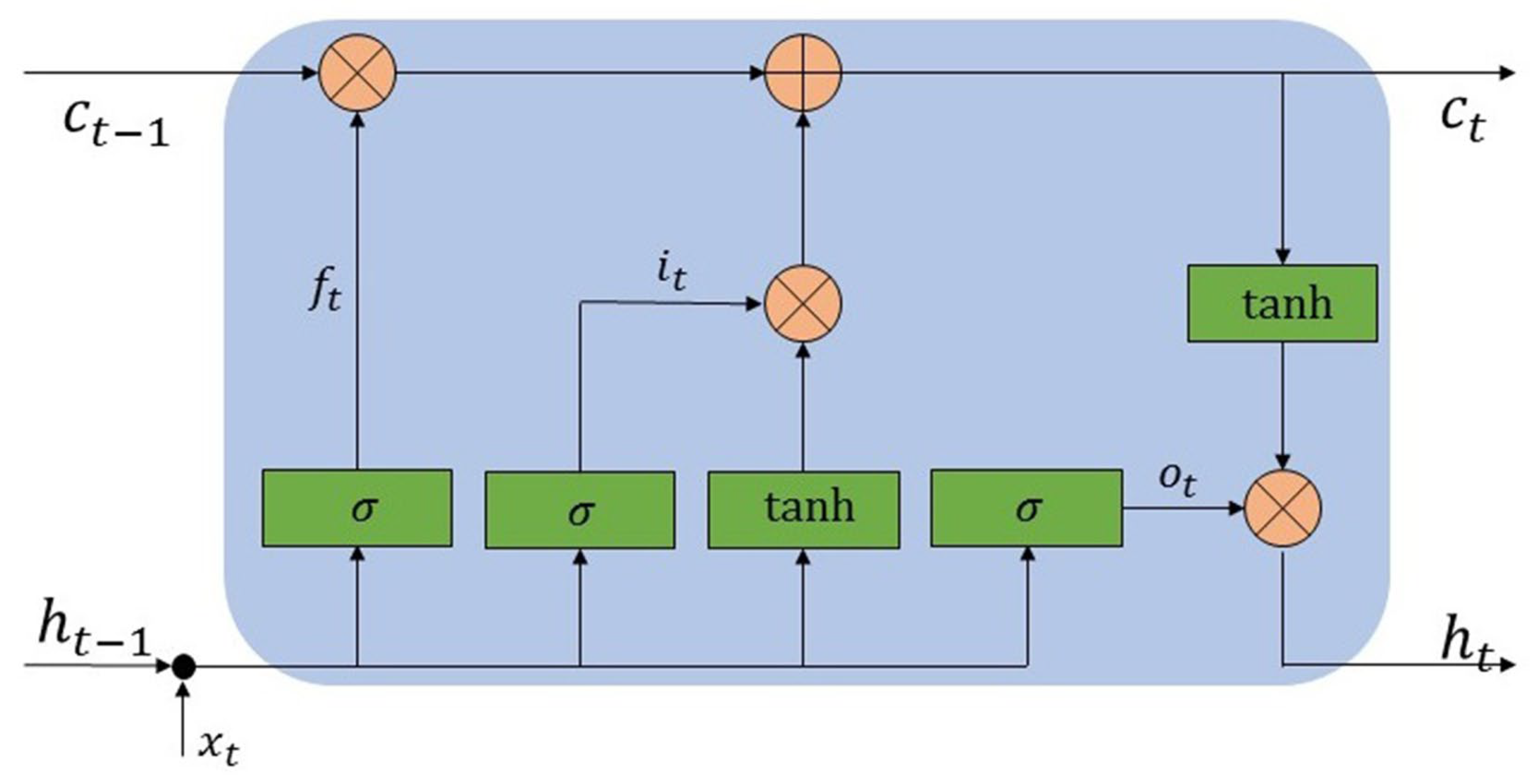
3.2. Long Short-Term Memory

Traditional neural networks cannot connect previous information with the current time step when dealing with long-term dependencies. However, as a special type of recurrent neural network, Long Short-Term Memory (LSTM) has a memory structure for learning long-term information [35]. The LSTM network realizes temporal memory function through the switch of the gate and can solve the problem of gradient vanishing and explosion in recurrent neural network effectively. The key to LSTM is the introduction of a gating unit system that stores historical information through the internal to allow the network to learn dynamically: that is, forgetting historical information or updating the cell state with new information.

The basic structure of an LSTM cell is illustrated in Figure 3, in which $x_t$ is the input vector, $h_t(h_{t-1})$ is the hidden state of the LSTM cell in time step $t(t-1)$, and $c_t(c_{t-1})$ is the cell state of the LSTM cell in time step $t(t-1)$. The structure of the LSTM cell shows that its cell state ($c_t$) and hidden state ($h_t$) are transferred to the next time step.

The LSTM cell has three gates (e.g., a forget gate ($f_t$), an input gate ($i_t$), and an output gate ($o_t$)) that maintain and adjust its cell ($c_t$) and hidden states ($h_t$). The forget gate ($f_t$) determines what information will be moved away from the cell state ($c_t$). The input gate ($i_t$) determines what new information will be stored in the cell state ($c_t$). The output gate ($o_t$) specifies what information from the cell state is used as output ($o_t$). In Figure 3, the cell state ($c_t$) and hidden state ($h_t$) of the LSTM cell are calculated as follows [54]:

$$f_t=\sigma (W_{xf}{x}_t+W_h{}_f{h}_{t-1}+b_f)$$

(4)

$$i_t=\sigma (W_{xi}{x}_t+W_{hi}{h}_{t-1}+b_i)$$

(5)

$${\widehat{c}}_t=\tanh (W_{xc}{x}_t+W_{hc}{h}_{t-1}+b_c)$$

(6)

$$c_t=f_t\otimes c_{t-1}+i_t\otimes {\widehat{c}}_t$$

(7)

$$o_t=\sigma (W_{xo}{x}_t+W_{ho}{h}_{t-1}+b_o)$$

(8)

$$h_t=o_t\otimes \tanh (c_t)$$

(9)

where $\sigma$ is the logistic sigmoidal function; $\otimes$ is the element-wise multiplication of two vectors; and $W_{xi}$, $W_{hi}$, $W_{xf}$, $W_{hf}$, $W_{xo}$, $W_{ho}$, $W_{xc}$, and $W_{hc}$ are the network weights matrices. Similarly, $b_i$, $b_f$, $b_o$, and $b_c$ are bias vectors. $f_t$, $i_t$, and $o_t$ are the vectors for the activation values of the forget gate, the input gate, and the output gate, respectively.

3.3. Chaos Sparrow Search Algorithm

3.3.1. Basic Sparrow Search Algorithm

The sparrow search algorithm is a new type of swarm intelligence optimization algorithm inspired by sparrow foraging behavior and anti-predation behavior [55]. It abstracts the sparrow foraging process into a discoverer–adder model and adds a reconnaissance and early warning mechanism. Assuming that N sparrows are found in a D-dimensional search space, the position of the i-th sparrow in the D-dimensional search space is $X_i=\left[x_{i,1},\cdots x_{i,d},\cdots x_{i,D}\right]$, where $i=1,2,\cdots N$, and $x_{i,d}$ represents the position of the i-th sparrow in the d-dimension.

The location of producers is updated as follows:

$$x_{i,d}^{t+1}=\left\{\begin{array}{l}{x}_{i,d}^t\exp \left(-\frac{i}{\alpha T}\right),R_2<ST\\ x_{i,d}^t+Q·\mathit{L},R_2\ge ST\end{array}\right.$$

(10)

where $t$ represents the current iteration number, $T$ represents the maximum number of iteration, $\alpha$ is a random number in the range of $(0,1)$, $Q$ is a random number and obeys $\left[0,1\right]$ normal distribution, $\mathit{L}$ is a row of multidimensional matrix where all elements are 1, $R_2\in \left(0,1\right]$ represents the warning value, and $ST\in \left[0.5,1\right]$ represents the safety value. If $R_2<ST$, then no natural enemies are observed nearby, the search environment is safe, and the discoverer implements an extensive search mode. If $R_2\ge ST$, then the sparrows detect natural enemies, and the entire population adjusts its search strategy and quickly moves to a safe area.

The scroungers’ locations is calculated according to formula (11):

$$x_{i,d}^{t+1}=\left\{\begin{array}{l}Q\cdot \exp \left(\frac{x_{w,d}^t-x_{i,d}^t}{i^2}\right),i>\frac{n}{2}\\ {\mathrm{x}}_{b,d}^{t+1}+\left|x_{i,d}^t-x_{b,d}^{t+1}\right|\cdot A^{+}\cdot L,i\le \frac{n}{2}\end{array}\right.$$

(11)

where $x_{w,d}^t$ represents the worst position of the sparrow in the d-th dimension at the t-th iteration, $x_{b,d}^{t+1}$ represents the best position of the sparrow in the d-th dimension at the $t+1$ iteration, and A is a $1\times d$ matrix with randomly assigned values of 1 or −1 for each element. If $i>n/2$, then the i-th follower did not receive food and has low adaptability and needs to fly to other areas to find food to obtain energy. If $i\le n/2$, then the i-th follower will randomly select a location nearby $x_{b,d}^{t+1}$ for foraging.

The position update formula of scouters is expressed as follows:

$$x_{i,d}^{t+1}=\left\{\begin{array}{l}{x}_{b,d}^t+\beta \cdot \left|x_{i,d}^t-x_{b,d}^t\right|,f_i\ne f_g\\ x_{i,d}^t+K\cdot \left(\frac{\left|x_{i,d}^t-x_{w,d}^t\right|}{\left|f_i-f_w\right|+\epsilon }\right),f_i=f_g\end{array}\right.$$

(12)

where $x_{b,d}^t$ represents the optimal position of the sparrow in the d-th dimension at the t-th iteration, $\beta$ is the step size control parameter, $K$ is a random number within $[-1,1]$, $f_i$ is the fitness value of the current sparrow, $f_g$ represents the current global optimal fitness value, $f_w$ represents the current global worst fitness value, and $\epsilon$ is a very small constant to avoid the state where the denominator becomes 0.

3.3.2. Improved Sparrow Algorithm

The population initialization of the sparrow search algorithm is a random generation method that causes the sparrow population to be unevenly distributed and easily falling into a local optimum [56]. However, chaotic mapping has the characteristics of randomness, ergodicity, and regularity [57]. Therefore, the chaotic map used in this article is the Tent map, and its formula is expressed as follows.

$$x_{i+1}=\left\{\begin{array}{l}2x_i,0\le x\le \frac{1}{2}\\ 2(1-x_i),\frac{1}{2}<x\le 1\end{array}\right.$$

(13)

By analyzing the Tent chaotic iterative sequence, we can find small periods and unstable period points. To prevent the Tent chaotic sequence from falling into small and unstable period points during iteration; the random variable $rand(0,1)\times \frac{1}{N}$ is introduced into the original Tent chaotic mapping formula. Hence, the improved Tent chaotic map expression is presented as follows:

$$x_{i+1}=\left\{\begin{array}{l}2x_i+rand\left(0,1\right)\times \frac{1}{N},0\le x\le \frac{1}{2}\\ 2\left(1-x_i\right)+rand\left(0,1\right)\times \frac{1}{N},\frac{1}{2}<x\le 1\end{array}\right.$$

(14)

where $N$ is the number of particles in the sequence, and $rand\left(0,1\right)$ is a random number in the range $\left[0,1\right]$. The introduction of random variable $rand(0,1)\times \frac{1}{N}$ not only still maintains the randomness, ergodicity, and regularity of the Tent chaotic map but it also can avoid having the iteration falling into small and unstable period points effectively.

When the fitness of an individual is greater than the average fitness of the population, a divergence trend will be observed. Therefore, chaotic disturbance is introduced to prevent the algorithm from falling into the local optimum and to improve the global search ability and optimization accuracy. The steps of chaotic disturbance are described as follows:

Step 1: Apply formula (14) to produce chaotic variable $x_d$.

Step 2: Carry chaotic variables to the solution space of the problem to be solved:

$$X_{new}^d=d_{\min }+(d_{\max }-d_{\min })\cdot x_d$$

(15)

where $d_{\min }$ is the minimum value of the d-th dimension variable $X_{new}^d$, and $d_{\max }$ is the maximum value of the d-th dimension variable $X_{new}^d$.

Step 3: Perform chaotic disturbance on the individual according to Formula (16):

$${X^{\prime }}_{new}=\frac{(X^{\prime }+X_{new})}{2}$$

(16)

where $X^{\prime }$ is the individual who needs chaotic disturbance, $X_{new}$ is the amount of chaotic disturbance generated, and ${X^{\prime }}_{new}$ is the individual after chaotic disturbance.

When the fitness of an individual is less than the average fitness of the population, it indicates that a clustering phenomenon occurs. The Gaussian distribution has strong local search ability. For optimization problems with a large number of local minima, it is conducive for the algorithm to find the global minima efficiently and accurately and to improve the robustness of the algorithm [58]. Therefore, this paper introduces Gaussian mutation, which is derived from the Gaussian distribution. Specifically, when performing mutation operation, we replace the original parameter value with a random number conforming to the normal distribution with mean $\mu$ and variance ${\sigma }^2$. The formula is expressed as follows:

$$mutation\left(x\right)=x\left[1+N\left(0,1\right)\right]$$

(17)

where $x$ is the original parameter value, $N(0,1)$ represents a normally distributed random number with $\mu =0$, and ${\sigma }^2=1$. $mutation\left(x\right)$ is the value after the Gaussian mutation.

3.4. Multiple Linear Regression

Multiple linear regression is a traditional prediction method. Compared with algorithms, such as BP and SVR, Multiple Linear Regression (MLR) has obvious advantages in the speed of the training process. At the same time, for the cyclical and smooth curve, compared with neural network and SVR, MLR can obtain accurate prediction values more easily. Its effect is similar to that of a neural network that uses a linear function as an activation function but does not require a cumbersome iterative training process and parameter adjustment. Therefore, for smooth low-frequency signals, MLR is a more suitable choice than other methods [59]. Its mathematical model can be represented as follows:

$$Y=X\times \beta +\mu$$

(18)

$$\left[\begin{array}{c}{y}_1\\ y_2\\ ⋮\\ y_n\end{array}\right]=\left[\begin{array}{cccc}1& x_{11}& \cdots & x_{1n}\\ 1& x_{21}& \cdots & x_{2n}\\ ⋮& ⋮& \ddots & ⋮\\ 1& x_{n1}& \cdots & x_{nn}\end{array}\right]\times \left[\begin{array}{c}{\beta }_0\\ {\beta }_1\\ ⋮\\ {\beta }_n\end{array}\right]+\left[\begin{array}{c}{\mu }_1\\ {\mu }_2\\ ⋮\\ {\mu }_n\end{array}\right]$$

(19)

where $y_i$ is the value of low-frequency signals, $x_{ij}$ represents the factors that affect the low-frequency signals, ${\beta }_0$ is a constant, ${\beta }_i(i=1,2,\cdots ,n)$ is the regression coefficient, and ${\mu }_i$ is the random variable. The solution of (18) can be easily obtained by using least-squares method, thereby yielding the following.

$$\widehat{\beta }={(X^{T}X)}^{-1}{X}^{T}Y$$

(20)

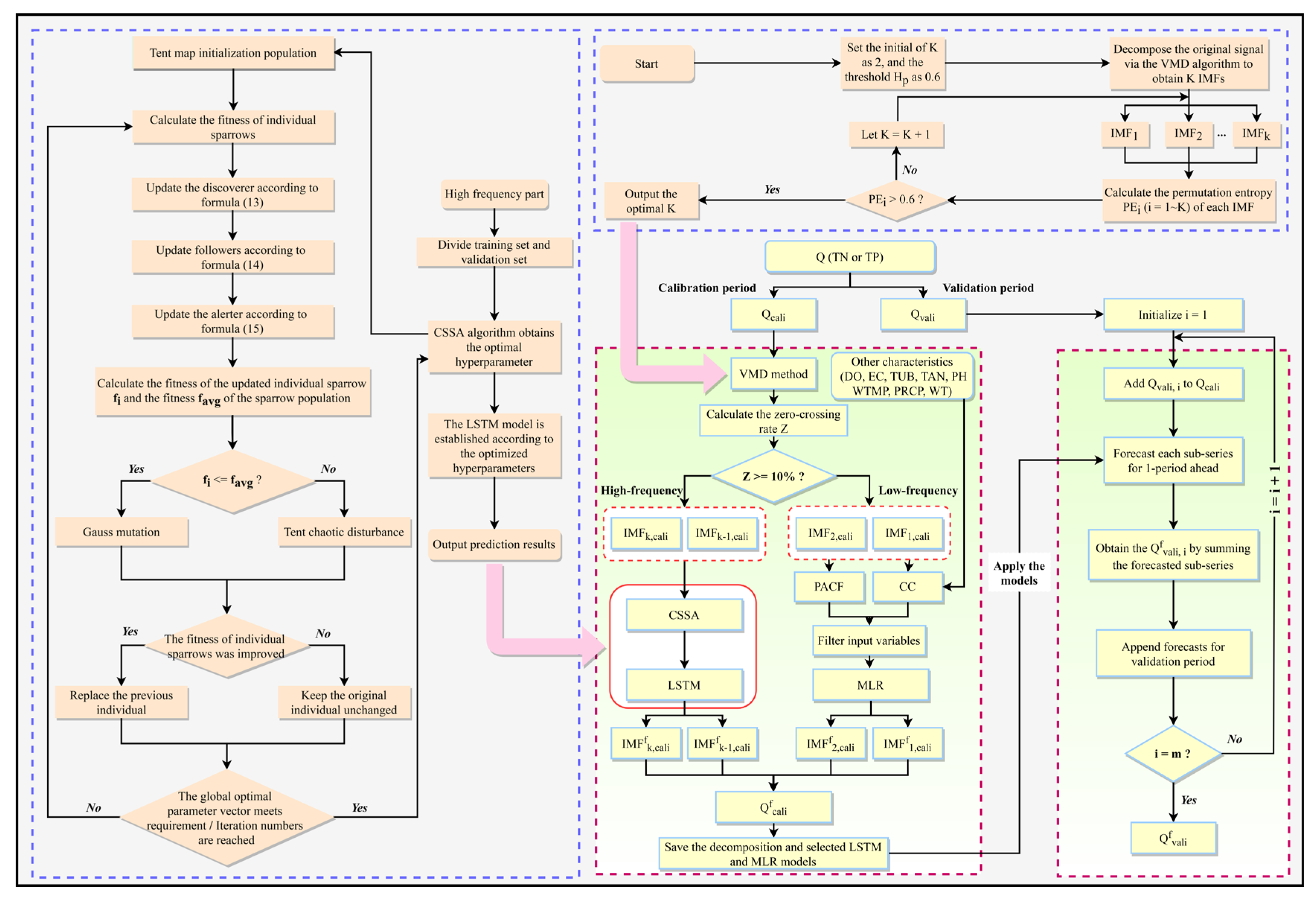
3.5. Water Quality Prediction Based on Hybrid Models

Due to many factors such as climate change and human activities, TN and TP in lakes and rivers are usually nonlinear and non-stationary time series. However, one problem with neural networks and other linear and nonlinear predictive models is that they cannot handle nonstationary data. Therefore, a VMD-based hybrid model (VMD-CSSA-LSTM-MLR or VCLM) is established in this paper. VMD is used to decompose the time series into multiple sub-sequences, and each sub-sequence is modeled separately. The sub-sequences obtained by VMD is relatively stable and can provide information about the time series data structure and its periodicity. Therefore, the performance of the prediction models is expected to be improved by providing useful information on various resolution levels.

However, it is worth noting that many literature used decomposition-based forecasting models to directly decompose the original time series and then divided the calibration set and the validation set. This process applies time series preprocessing techniques directly to a complete time series, thus transferring some information from the validation period to the training process of the data-driven model, resulting in “hindcasting experiments”, and the time series prediction results at a specific moment are calculated using future information that would not be available at that specific moment in a practical real practical application of time series forecasting known as “forecasting experiments” [60,61]. Obviously, this method is unreasonable, so this paper chooses to divide the calibration set and validation set first, and then it decomposes them to avoid using future information. The specific implementation steps are detailed as follows.

Step 1: Divide the entire data $Q$ (TN or TP) into the calibration period $Q_{cali}$ and the validation period $Q_{vali}$ (with 70% and 30% of the overall data, respectively, in the work), and initialize the data number in the validation period $i=1$.

Step 2: Decompose $Q_{cali}$ into $K$ IMFs using an improved adaptive VMD algorithm (Section 3.1.2).

Step 3: According to Formula (21), the zero-crossing rate of each IMFs is calculated and divided into high-frequency and low-frequency parts with 10% as the limit. The calculation equation is detailed as follows:

$$Z=\frac{n_{zero}}{N}\times 100\%$$

(21)

where $Z$ represents the zero-crossing rate, $n_{zero}$ represents the number of zero crossings (that is, if the adjacent signal values have different signs, then it means one zero crossing), and $N$ represents the signal length.

Step 4: The low-frequency components are predicted by MLR, and the input variables of the model are determined according to the correlation coefficient (CC) and the partial autocorrelation function (PACF).

Step 5: The high-frequency components are predicted by LSTM. The hyperparameters of the LSTM model are optimized using CSSA.

Step 6: Obtain $Q_{cali}^f$ by summing the outputs of all selected LSTM and MLR models.

Step 7: Save the selected LSTM and MLR models to forecast each subsequence for 1-period ahead, and $Q_{vali,i}^f$ is obtained by summing the forecasted sub-sequences.

Step 8: If $i=m$, stop and output $Q_{vali}^f$. Otherwise, let $i=i+1$ and append $Q_{vali,i}$ into the calibration data, and then repeat Steps 2 to 7.

The implementation of the hybrid prediction model is shown in Figure 4.

3.6. Model Performance Evaluation

To objectively evaluate the prediction accuracy of the model, five statistical indicators are used: mean absolute error (MAE), mean absolute percentage error (MAPE), root mean square error (RMSE), Nash–Sutcliffe efficiency coefficient (NSE), and Kling–Gupta efficiency (KGE). NSE is a normalized statistic that determines the relative magnitude of the residual variance compared to the measured data variance. The KGE, which has been introduced as an improvement of the widely used NSE, considers different types of model errors, namely, the error in the mean, the variability, and the dynamics [62]. The definitions of these statistics are given as follows:

$$MAE=\frac{1}{N}{\displaystyle \sum _{\mathrm{i}=0}^N\left|O_i-P_i\right|}$$

(22)

$$MAPE=\frac{1}{N}{\displaystyle \sum _{i=0}^N\frac{\left|O_i-P_i\right|}{P_i}}\times 100\%$$

(23)

$$RMSE=\sqrt{\frac{1}{N}{\displaystyle \sum _{i=0}^N{\left(O_i-P_i\right)}^2}}$$

(24)

$$NSE=1-\frac{{\displaystyle \sum _{i=0}^N{\left(O_i-P_i\right)}^2}}{{\displaystyle \sum _{i=0}^N{\left(O_i-\overline{O}\right)}^2}}$$

(25)

$$KGE=1-\sqrt{{\left[1-r\left(O_i,P_i\right)\right]}^2+{\left[1-\frac{\overline{O}}{\overline{P}}\right]}^2+{\left[1-\frac{\sigma \left(O_i\right)}{\sigma \left(P_i\right)}\right]}^2}$$

(26)

where $O_i$ is the measured value, $P_i$ is the simulated value, $\overline{O}$ is the measured average, $\overline{P}$ is the average of the simulated value, $N$ is the number of measured values, $r\left(·\right)$ is the Pearson correlation coefficient, and $\sigma \left(·\right)$ is the standard deviation.

4. Results

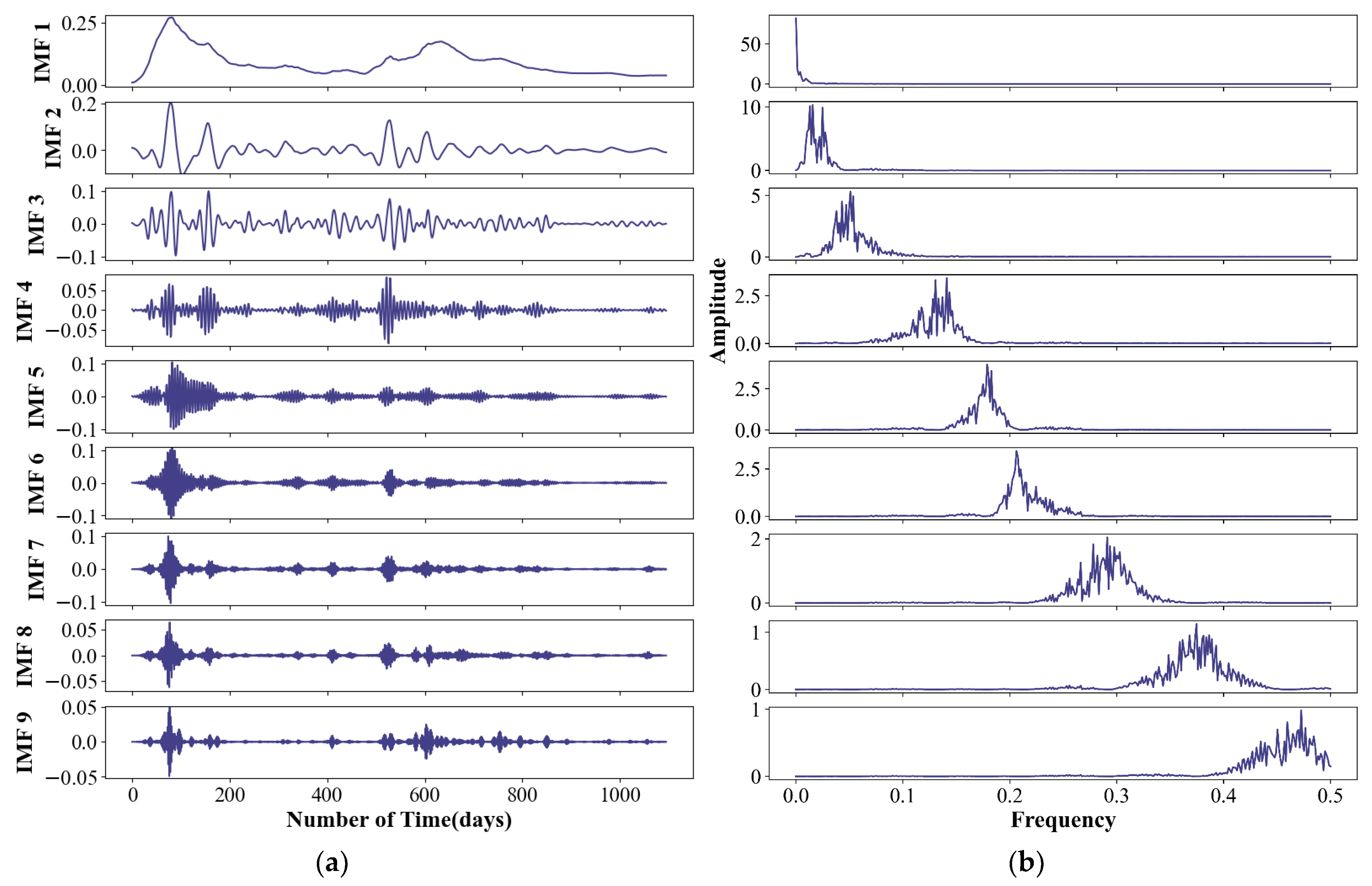
4.1. Decomposition Results Using VMD

According to Figure 2, it can be seen intuitively that TN and TP time series of the four stations have nonlinear and non-stationary characteristics. To solve this problem, the improved VMD method described in Section 3.1 is used to decompose the daily TN and TP sequences of the four aforementioned stations. The parameters of the VMD decomposition include modal number $K$, penalty factor $\alpha$, fidelity $\tau$, and convergence criterion $\epsilon$. The $K$ value can be determined adaptively according to the calculated PE, $\tau$ and $\epsilon$ select default values, and $\alpha$ is determined to be 1000 after repeated trials. The result of decomposition and center frequency of TN data at DC station are shown in Figure 5. VMD technology is used to decompose the calibration set time series into nine IMF components with different frequencies (Figure 5), which show the nonlinearity, trend, periodicity, and other characteristics of the original sequence. The VMD method can effectively eliminate non-stationary characteristics in the original sequence, which contributes to improve the prediction accuracy of the model significantly [63].

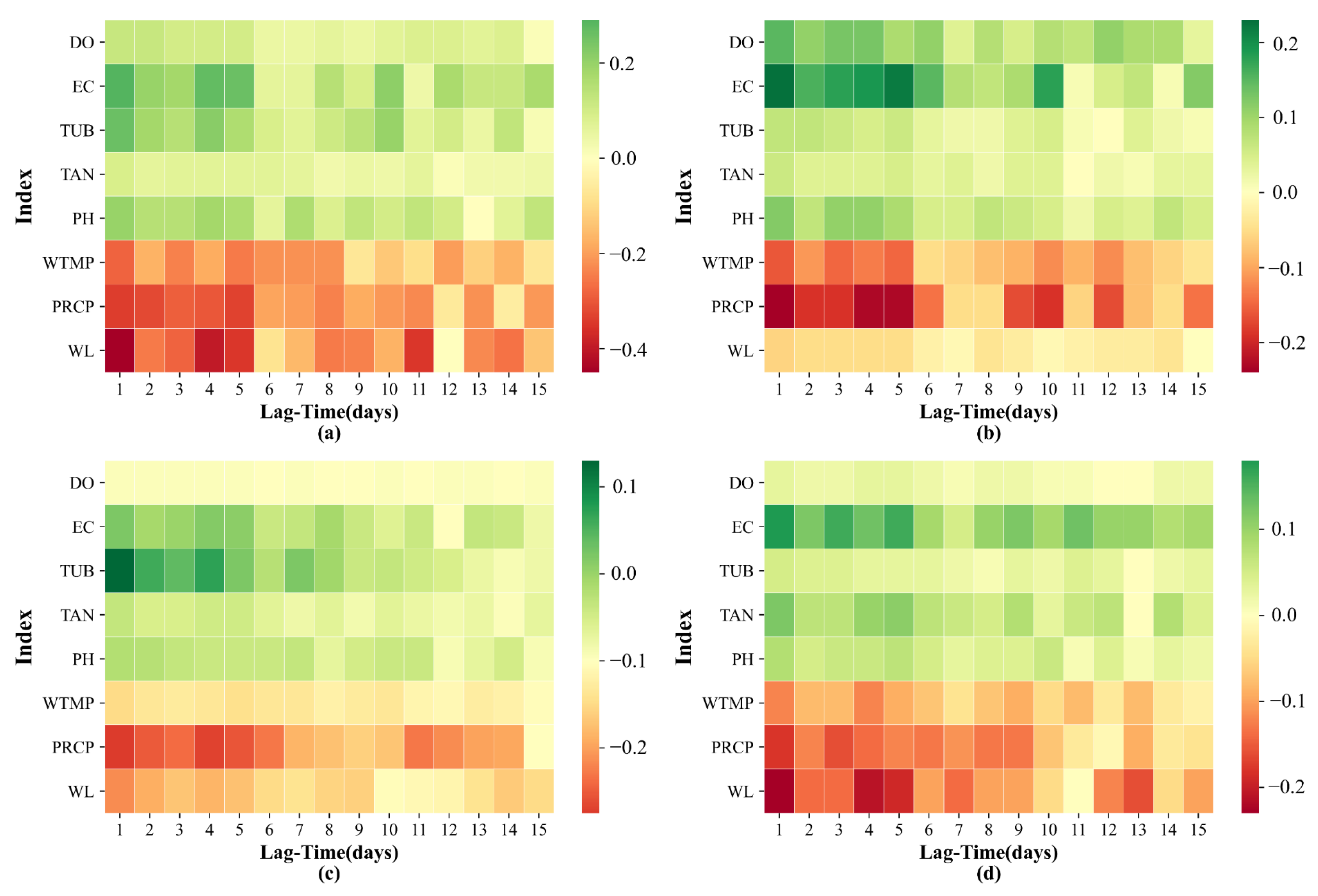
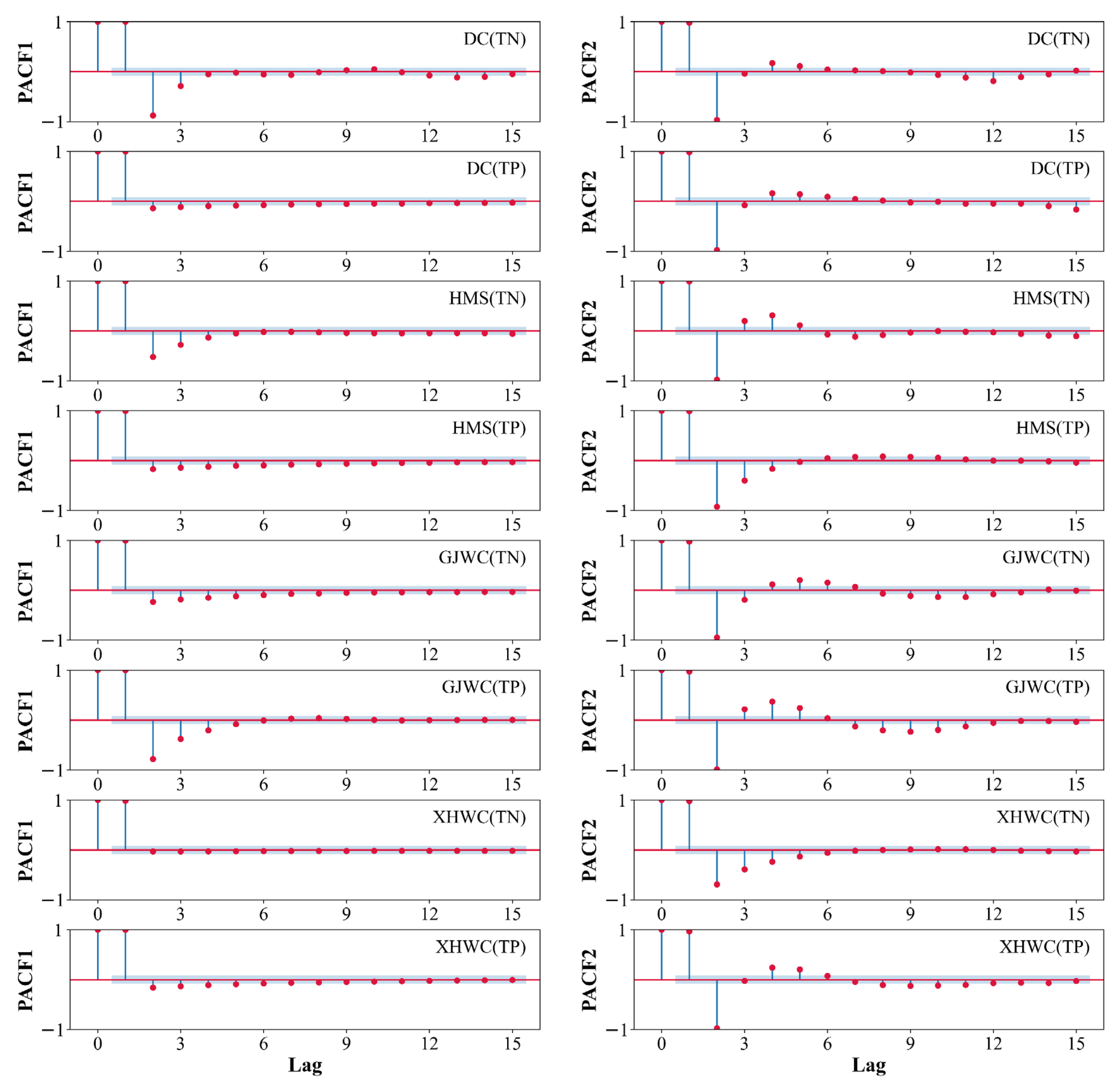
4.2. Model Building and Inputs

According to formula (21), the zero-crossing rate of each IMF component obtained by the VMD decomposition is calculated according to the principle that the part exceeding 10% is high-frequency component, and the part less than 10% is a low-frequency component. Finally, IFM1 and IFM2 are determined to be low-frequency components, and other IMFs are high-frequency components. MLR is used to predict the low-frequency components, the correlation coefficients between the low-frequency components and eight features (DO, EC, TUB, TAN, PH, WTMP, PRCP, and WL) with a time lag of 15 days at DC Station are shown in Figure 6, and the features with an absolute value of the correlation coefficient greater than 0.3 are selected as regression factors. In addition, for time series forecasting, its time lag usually needs to be considered. To determine the impact of an appropriate time lag on the current $t$ time interval, the partial autocorrelation function (PACF) is used as a potential indicator to identify the appropriate input variables. Generally, the following criteria are often used in practice: Assuming that the input variable is $x_i$, (1) when the PACF value of the variable $x_{i-k}$ at the lag k is out of the 95% confidence interval, it is selected as the input variable, and (2) the previous value $x_{i-1}$ will be regarded as an input when all PACF values fall inside the 95% confidence interval [63,64,65]. Figure 7 shows the PACF of low-frequency components, and

Table 1. Input variables of MLR model for each station.

Station	Decomposed IMFs	No. of Inputs	Input Variables	Output
DC(TN)	IMF1	9	$\begin{array}{l}{x}_1(t-1),x_1(t-2),x_1(t-3),PRCP(t-1),PRCP(t-2),\\ PRCP(t-4),PRCP(t-5),WL(t-1),WL(t-4)\end{array}$	$x_1(t)$
	IMF2	7	$\begin{array}{l}{x}_2(t-1),x_2(t-2),x_2(t-4),x_2(t-5),x_2(t-11),\\ x_2(t-12),x_2(t-13)\end{array}$	$x_2(t)$
DC(TP)	IMF1	8	$\begin{array}{l}{x}_1(t-1),x_1(t-2),x_1(t-3),TUB(t-1),TUB(t-2),\\ TUB(t-4),PRCP(t-1),PRCP(t-4)\end{array}$	$x_1(t)$
	IMF2	6	$\begin{array}{l}{x}_2(t-1),x_2(t-2),x_2(t-3),x_2(t-4),x_2(t-5),\\ x_2(t-6)\end{array}$	$x_2(t)$
HMS(TN)	IMF1	9	$\begin{array}{l}{x}_1(t-1),x_1(t-2),x_1(t-3),x_1(t-4),DO(t-1),\\ EC(t-1),TUB(t-1),WL(t-1),WL(t-2)\end{array}$	$x_1(t)$
	IMF2	7	$\begin{array}{l}{x}_2(t-1),x_2(t-2),x_2(t-3),x_2(t-4),x_2(t-5),\\ EC(t-1),EC(t-3)\end{array}$	$x_2(t)$
HMS(TP)	IMF1	7	$\begin{array}{l}{x}_1(t-1),x_1(t-2),x_1(t-3),x_1(t-4),DO(t-1),\\ WTMP(t-1),WL(t-1)\end{array}$	$x_1(t)$
	IMF2	7	$\begin{array}{l}{x}_2(t-1),x_2(t-2),x_2(t-3),x_2(t-4),PRCP(t-1),\\ PRCP(t-2),PRCP(t-3)\end{array}$	$x_2(t)$
GJWC(TN)	IMF1	9	$\begin{array}{l}{x}_1(t-1),x_1(t-2),x_1(t-3),x_1(t-4),x_1(t-5),\\ DO(t-1),TUB(t-1),TAN(t-1),WTMP(t-1)\end{array}$	$x_1(t)$
	IMF2	9	$\begin{array}{l}{x}_2(t-1),x_2(t-2),x_2(t-3),x_2(t-4),x_2(t-5),\\ x_2(t-6),x_2(t-9),x_2(t-10),x_2(t-11)\end{array}$	$x_2(t)$
GJWC(TP)	IMF1	8	$\begin{array}{l}{x}_1(t-1),x_1(t-2),x_1(t-3),x_1(t-4),DO(t),\\ TUB(t-1),TUB(t-2),PH(t-1)\end{array}$	$x_1(t)$
	IMF2	5	$x_2(t-1),x_2(t-2),x_2(t-3),x_2(t-4),x_2(t-5)$	$x_2(t)$
XHWC(TN)	IMF1	7	$\begin{array}{l}{x}_1(t-1),TUB(t-1),TUB(t-3),TAN(t-1),\\ WTMP(t-1),WL(t-1),WL(t-2)\end{array}$	$x_1(t)$
	IMF2	7	$\begin{array}{l}{x}_2(t-1),x_2(t-2),x_2(t-3),x_2(t-4),x_2(t-5),\\ TAN(t-1),TAN(t-2)\end{array}$	$x_2(t)$
XHWC(TP)	IMF1	6	$\begin{array}{l}{x}_1(t-1),TUB(t-1),TAN(t-1),WTMP(t-1),\\ WTMP(t-2),WL(t-1)\end{array}$	$x_1(t)$
	IMF2	4	$x_2(t-1),x_2(t-2),x_2(t-4),x_2(t-5)$	$x_2(t)$

shows the input variables of the MLR model.

The LSTM model is used for modeling high-frequency components. By analyzing the correlation coefficients between the eight features and each high-frequency component, it is found that the correlation between them is very low. This result indicates that VMD can decompose some potential features of the time series, which may require more data of relevant influencing factors to further verify their relationship with high frequency components. Wang et al. [66] used ensemble empirical mode decomposition to decompose the runoff into different frequency components, comprehensively considered 130 climatic phenomenon indices, and conducted teleconnection analysis of each frequency component according to the correlation coefficient. The results show that each component has practical physical significance. The eight features used in this paper have good correlation with low-frequency components and low correlation with high-frequency components. Therefore, the input of high-frequency components only uses its lag data as the inputs of the LSTM model. The critical parameters of LSTM, such as the length of the sliding time window, the number of hidden layer neurons, dropout ratio, learning rate, and batch size, are the prerequisites for the prediction performance of the LSTM model. Therefore, CSSA is used to automatically calibrate the parameters of the LSTM model. CSSA-LSTM not only inherits the advantages of LSTM but also utilizes the advantages of the CSSA for solving optimization problems, where the foraging process of the sparrow population can interact with the training process of the LSTM and optimize the hyperparameters of the LSTM model. The number of nodes in the input layer of the LSTM model is equal to the number of input variables, the number of nodes in the output layer is fixed at 1, and the number of hidden layers is generally set to two. The hyperparameters of the LSTM model to be optimized include the length of the sliding time window (LW), the number of hidden layer neurons (NN), dropout ratio (DR), learning rate (LR), and batch size (BS), and their specified search ranges are (1, 30), (10, 150), (0, 1), (0.001, 1), and (1, 150), respectively. Furthermore, LW, NN, and BS are discrete variables, and DR and LR are continuous variables.

4.3. Comparison of Different Metaheuristic Optimization Algorithms

To verify the effectiveness and superiority of the CSSA algorithm, the performance of the proposed CSSA in identifying the optimal LSTM configuration is compared with five classical search methods, i.e., SSA, GWO [67], PSO [68], GSA [69], and FPA [70]. The parameter settings of the baseline models are provided in

Table 2. Parameter settings of search methods.

Methods	Parameter Settings
CSSA	The proportion of producers is 20%, and the proportion of scouters is 20%
SSA	The proportion of producers is 20%, and the proportion of scouters is 20%
GWO	Step size $A=(2\times rand-1)\times a$, where $\alpha$ linearly decreases from 2 to 0, $rand\in (0,1)$, search parameter $C=2\times rand$
PSO	Cognitive component $c_1=1.4962$, social component $c_2=1.4962$, inertia weight $\alpha =20$
GSA	Initial gravitational constant $G_0=100$, search parameter $\alpha =20$
FPA	Switch probability $=0.8$, step size $L$ for global pollination drawn from a Levy flight distribution, step size $\epsilon$ for local pollination drawn from a uniform distribution within $[0,1]$

. The following settings are used for each experiment to ensure a fair comparison, i.e., the maximum number of function evaluations = population size (30) × the maximum number of iterations (100). We conduct our experiments using a Tesla K80 GPU with 12 GB RAM. Moreover, we conduct 10 independent runs for each experiment to mitigate the impact of random factors on the evaluation.

4.3.1. Experimental Settings

A total of 1096 TN data in DC Station were selected, with the first 70% as calibration set and the last 30% as validation set. The correlation coefficients between TN and 8 features were calculated, and the features with absolute correlation coefficients greater than 0.3 were selected as the input variable of LSTM. Different intelligent optimization algorithms are used to optimize the hyperparameters of LSTM, and their specific hyperparameter search range is shown in Section 4.2. In addition, considering the running speed and prediction accuracy of the LSTM model, a two-layer LSTM was selected for modeling, and the Adam optimizer was applied in the training process while the RMSE was adopted as the fitness score to evaluate the performance of LSTM.

4.3.2. Comparison of Results

Three performance indicators were used to evaluate the effectiveness of the CSSA-LSTM model, i.e., MAE, RMSE and MAPE. The respective results over ten independent runs are presented in

Table 3. The MAE results over 10 independent runs.

Run	CSSA	SSA	GWO	PSO	GSA	FPA
1	0.1116	0.1516	0.1616	0.1624	0.1191	0.1086
2	0.1024	0.1530	0.1438	0.1052	0.1158	0.1393
3	0.1339	0.1139	0.1601	0.1566	0.1087	0.1453
4	0.1203	0.1229	0.1463	0.1309	0.1508	0.1419
5	0.1464	0.1592	0.1197	0.1240	0.1412	0.1255
6	0.1056	0.1520	0.1625	0.1322	0.1459	0.1623
7	0.1387	0.1231	0.1044	0.1608	0.1430	0.1153
8	0.1428	0.1185	0.1485	0.1527	0.1454	0.1451
9	0.1381	0.1219	0.1231	0.1208	0.1207	0.1297
10	0.1174	0.1089	0.1097	0.1317	0.1318	0.1409
Avg.	0.1257	0.1325	0.1380	0.1377	0.1354	0.1325

,

Table 4. The MAPE results over 10 independent runs.

Run	CSSA	SSA	GWO	PSO	GSA	FPA
1	0.1210	0.1203	0.1458	0.1300	0.1399	0.1426
2	0.1055	0.1488	0.1085	0.1480	0.1245	0.1263
3	0.1128	0.1451	0.1463	0.1208	0.1040	0.1415
4	0.1167	0.1080	0.1219	0.1072	0.1255	0.1678
5	0.1403	0.1341	0.1633	0.1258	0.1481	0.1108
6	0.0988	0.1323	0.1447	0.1253	0.1297	0.1710
7	0.1238	0.1482	0.1482	0.1554	0.1392	0.1342
8	0.1371	0.1103	0.1502	0.1525	0.1203	0.1405
9	0.1230	0.1484	0.1618	0.1403	0.1304	0.1196
10	0.1019	0.1267	0.1474	0.1334	0.1135	0.1004
Avg.	0.1181	0.1322	0.1438	0.1339	0.1275	0.1355

and

Table 5. The RMSE results over 10 independent runs.

Run	CSSA	SSA	GWO	PSO	GSA	FPA
1	0.1612	0.1714	0.1900	0.1504	0.1860	0.1882
2	0.1789	0.1718	0.1781	0.1738	0.1825	0.1809
3	0.1608	0.1793	0.1650	0.2042	0.1710	0.1607
4	0.1659	0.1635	0.1918	0.1619	0.1836	0.1692
5	0.1845	0.1662	0.1908	0.1876	0.1744	0.1959
6	0.1610	0.1714	0.1765	0.1658	0.1635	0.1647
7	0.1472	0.1953	0.1829	0.1843	0.1607	0.1664
8	0.1622	0.1426	0.2187	0.1782	0.1473	0.1577
9	0.1580	0.1830	0.1931	0.1763	0.1825	0.1591
10	0.1567	0.1718	0.1963	0.1959	0.1488	0.1724
Avg.	0.1637	0.1716	0.1883	0.1778	0.1702	0.1724

, where CSSA-SVR shows better optimization performance than the other five optimization algorithms. Compared with SSA-LSTM, CSSA-LSTM decreased by 5.13%, 10.67%, and 4.61% in terms of the average MAE, RMSE, and MAPE, respectively. The results show that the improved SSA algorithm is effective and can improve the optimization performance of the algorithm significantly. Meanwhile, compared with GWO-LSTM, PSO-LSTM, GSA-LSTM, and FPA-LSTM, the average MAE, RMSE, and MAPE of CSSA-LSTM decreased by 5.13~8.91%, 7.37~17.87%, and 3.82~13.06%, respectively.

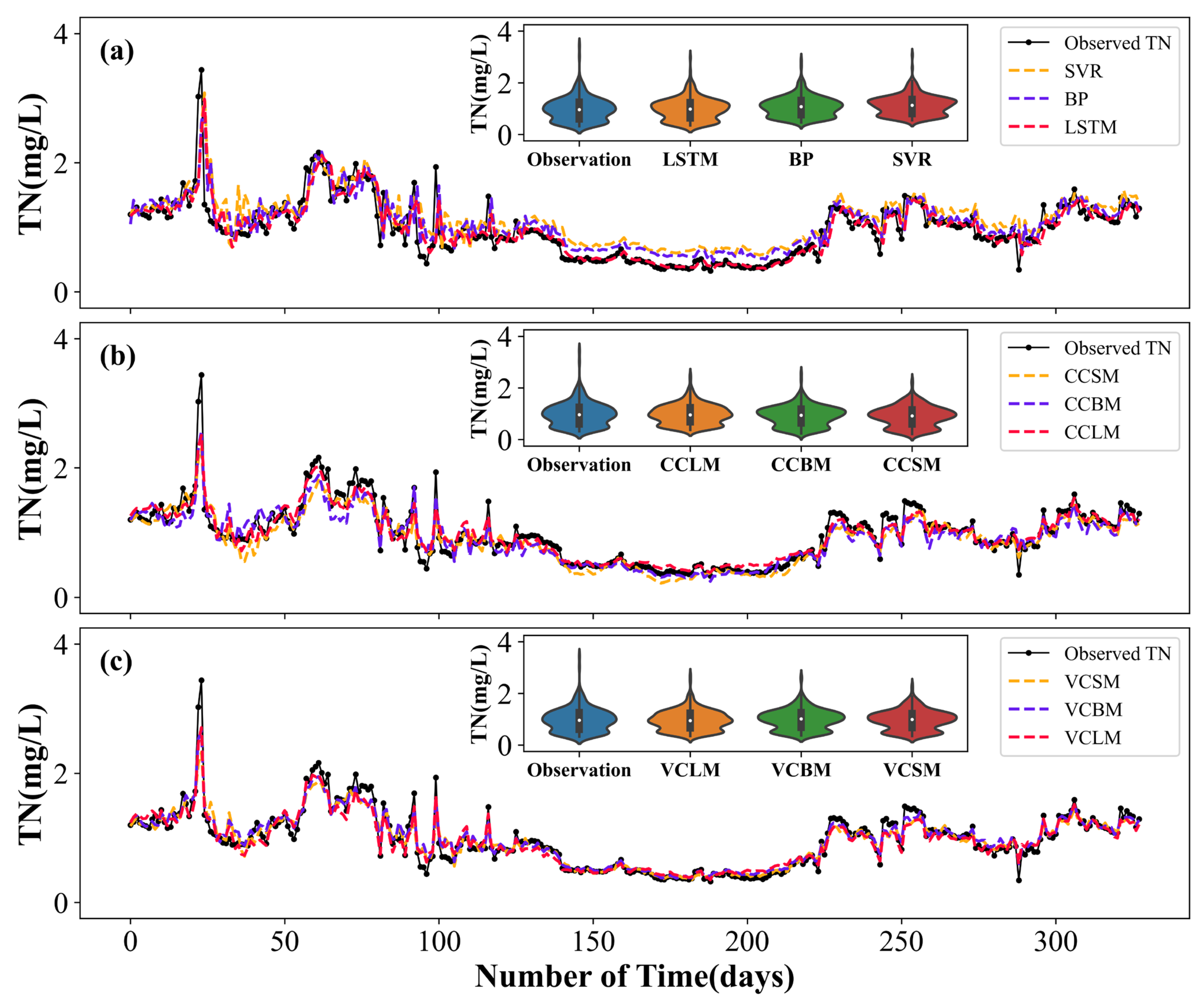
4.4. Comparison of the Results of Various Prediction Models

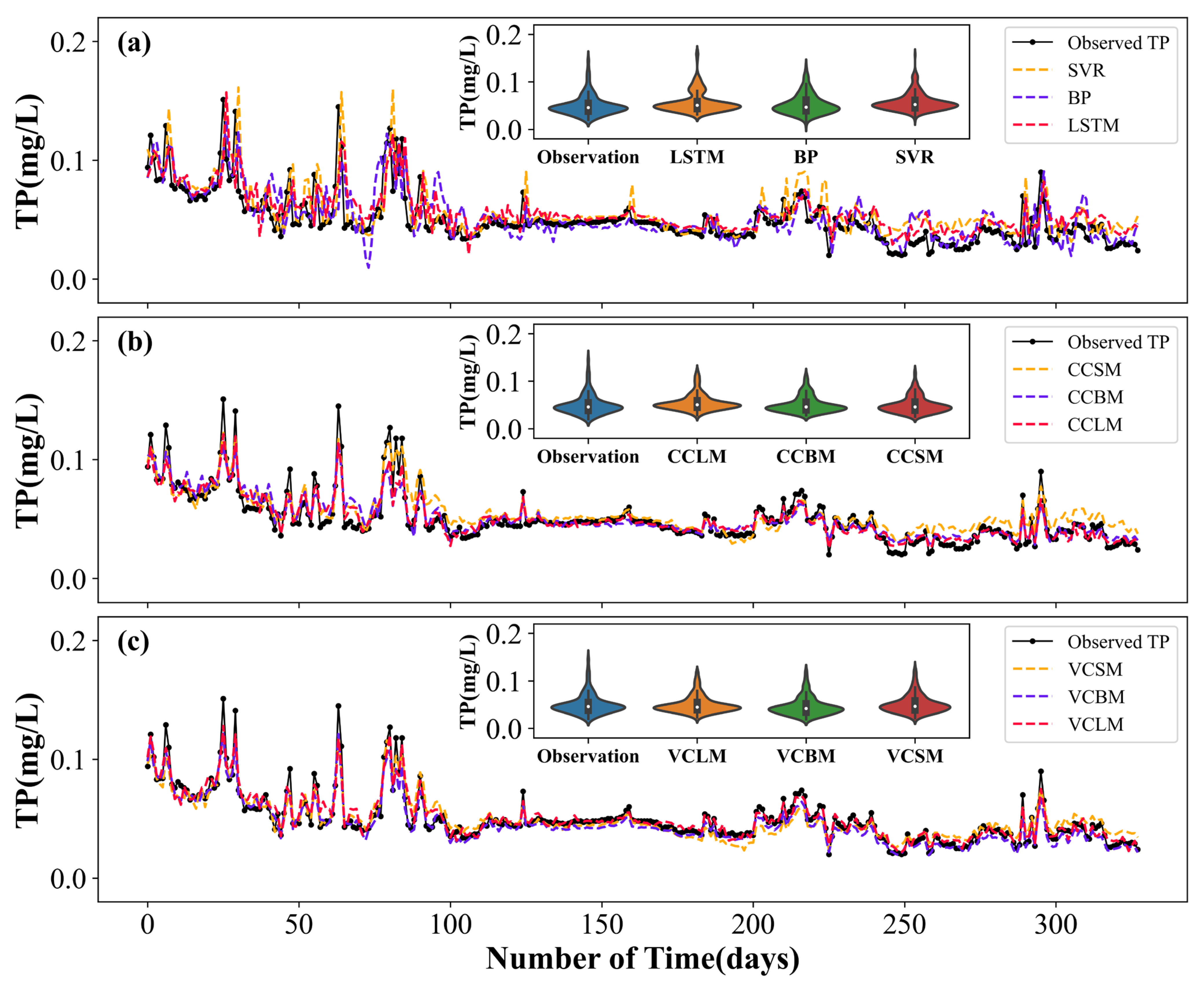
4.4.1. Water Quality Prediction Performance with Standalone Model

Three standalone prediction models, namely, SVR, BP, and LSTM, are compared. For a reasonable comparison, the hyperparameters of the three models are optimized by CSSA.

Table 6. Performance comparison of each model.

Station	Item	VCLM	VCL	VCBM	VCSM	CCLM	CCBM	CCSM	LSTM	BP	SVR
DC (TN)	MAE	0.0493	0.0523	0.0637	0.0678	0.0887	0.0909	0.0926	0.1080	0.1120	0.1254
	MAPE	5.34%	6.15%	7.46%	7.73%	9.16%	9.77%	10.29%	11.46%	11.67%	14.14%
	RMSE	0.0640	0.0795	0.0871	0.0922	0.1136	0.1174	0.1227	0.1489	0.1568	0.1766
	NSE	0.9346	0.9015	0.8790	0.8452	0.7910	0.7614	0.7459	0.5483	0.5106	0.4052
	KGE	0.8909	0.8509	0.8001	0.8127	0.7653	0.7448	0.7352	0.5046	0.4694	0.3899
DC (TP)	MAE	0.0025	0.0031	0.0033	0.0039	0.0041	0.0043	0.0043	0.0049	0.0051	0.0049
	MAPE	6.84%	7.68%	8.23%	9.06%	9.94%	10.12%	10.05%	12.68%	13.79%	13.46%
	RMSE	0.0030	0.0037	0.0046	0.0051	0.0056	0.0059	0.0061	0.0078	0.0081	0.0115
	NSE	0.9247	0.8829	0.8402	0.8034	0.7520	0.7214	0.7015	0.4873	0.4418	0.4219
	KGE	0.8994	0.8673	0.8257	0.8124	0.6881	0.6497	0.6649	0.3986	0.3327	0.3488
HMS (TN)	MAE	0.1175	0.1215	0.1435	0.1507	0.1482	0.1681	0.1571	0.1875	0.2179	0.2008
	MAPE	6.05%	6.83%	7.23%	7.67%	7.47%	8.21%	8.04%	10.49%	12.38%	11.67%
	RMSE	0.1584	0.1797	0.1979	0.2012	0.2429	0.2376	0.2828	0.3232	0.3457	0.3891
	NSE	0.9058	0.8747	0.8427	0.7995	0.8078	0.7714	0.7864	0.5288	0.4050	0.4331
	KGE	0.9086	0.8994	0.8758	0.8359	0.8140	0.7349	0.7752	0.4230	0.3628	0.3472
HMS (TP)	MAE	0.0054	0.0064	0.0081	0.0083	0.0092	0.0098	0.0104	0.0117	0.0119	0.0126
	MAPE	8.50%	9.21%	10.57%	10.33%	13.76%	14.44%	14.29%	19.40%	21.95%	22.62%
	RMSE	0.0079	0.0083	0.0086	0.0108	0.0112	0.0121	0.0134	0.0186	0.0191	0.0195
	NSE	0.9185	0.9058	0.8953	0.8943	0.8026	0.7694	0.7768	0.5944	0.5144	0.4843
	KGE	0.9275	0.8901	0.8605	0.8677	0.7844	0.7814	0.7294	0.6012	0.5135	0.5029
GJWC (TN)	MAE	0.1774	0.1828	0.2093	0.2576	0.2640	0.2694	0.2748	0.3018	0.3409	0.3267
	MAPE	15.82%	16.72%	18.65%	19.81%	24.31%	23.64%	24.49%	26.79%	30.79%	28.94%
	RMSE	0.1785	0.2406	0.2253	0.2891	0.3696	0.4180	0.4462	0.4798	0.4991	0.4945
	NSE	0.8864	0.8621	0.8545	0.8367	0.7222	0.7068	0.6972	0.4819	0.4131	0.4324
	KGE	0.8266	0.8205	0.7958	0.7864	0.6893	0.6449	0.6257	0.4246	0.3826	0.4091
GJWC (TP)	MAE	0.0078	0.0085	0.0095	0.0092	0.0121	0.0131	0.0134	0.0185	0.0199	0.0201
	MAPE	17.47%	18.69%	20.34%	20.49%	22.84%	23.35%	23.61%	27.63%	29.83%	32.47%
	RMSE	0.0096	0.0106	0.0118	0.0134	0.0147	0.0165	0.0195	0.0265	0.0305	0.0312
	NSE	0.9058	0.8932	0.8895	0.8823	0.7853	0.7442	0.7322	0.4334	0.4266	0.4057
	KGE	0.8849	0.8511	0.8301	0.8349	0.7501	0.6981	0.7246	0.4291	0.3537	0.3139
XHWC (TN)	MAE	0.1647	0.1688	0.2019	0.2278	0.2886	0.3066	0.3115	0.3554	0.3682	0.3788
	MAPE	5.16%	5.42%	6.37%	6.44%	7.64%	7.82%	7.78%	8.94%	9.21%	9.42%
	RMSE	0.2155	0.2519	0.2898	0.4875	0.4390	0.4738	0.5090	0.6581	0.8389	0.7670
	NSE	0.9510	0.9252	0.9034	0.8826	0.8337	0.8249	0.7977	0.5975	0.5521	0.5228
	KGE	0.9187	0.9081	0.8973	0.8671	0.8218	0.8114	0.8161	0.5664	0.4843	0.4590
XHWC (TP)	MAE	0.0033	0.0036	0.0041	0.0044	0.0052	0.0054	0.0054	0.0065	0.0069	0.0072
	MAPE	10.50%	11.81%	12.29%	12.38%	15.38%	15.63%	15.82%	19.63%	20.37%	22.38%
	RMSE	0.0043	0.0052	0.0049	0.0056	0.0063	0.0065	0.0081	0.0102	0.0118	0.0155
	NSE	0.9463	0.9227	0.9192	0.9088	0.8647	0.8497	0.8324	0.5294	0.4864	0.4429
	KGE	0.8536	0.8314	0.8065	0.8143	0.8518	0.7932	0.8146	0.5577	0.4219	0.4597

shows the prediction performance of TN and TP using three standalone models for four stations, and the specific values are shown in Table 6.

For the prediction of TN, the overall effect of LSTM (average MAE, MAPE, RMSE, NSE, and KGE were 0.2382, 14.42%, 0.4025, 0.5891, and 0.5297, respectively) is significantly better than BP (average MAE, MAPE, RMSE, NSE, and KGE were 0.2598, 16.01%, 0.4601, 0.5202, and 0.4748, respectively) and SVR (average MAE, MAPE, RMSE, NSE, and KGE were 0.2579, 16.04%, 0.4568, 0.4984, and 0.4513, respectively). Similarly, in terms of TP prediction, the overall effect of LSTM (average MAE, MAPE, RMSE, NSE, and KGE were 0.0104, 19.84%, 0.0158, 0.5611, and 0.5467, respectively) is still better than those of BP (average MAE, MAPE, RMSE, NSE, and KGE were 0.0110, 21.49%, 0.0174, 0.5173, and 0.4555, respectively) and SVR (average MAE, MAPE, RMSE, NSE, and KGE were 0.0112, 22.73%, 0.0194, 0.4887, and 0.4563, respectively). The predicted performances of BP and SVR are relatively close. The results show that compared with traditional BP and SVR, LSTM has higher prediction accuracy, wider applicability, and stronger stability for non-stationary and nonlinear time series. Figure 8a and Figure 9b show the prediction curves of TN and TP by three standalone models at DC station. Figure 8a and Figure 9b show that the three models can roughly predict the trend. However, the prediction effect of some points with large fluctuations is very poor. An obvious “lag” phenomenon can also be observed in the prediction result of the model; that is, the prediction result of the model is closer to the prediction result of the previous day. This finding indicates that the internal law of water quality parameter time series with strong randomness and instability cannot be learned well by a standalone model.

4.4.2. Water Quality Prediction Performance with CEEMDAN Decomposition

Aiming at the problem that standalone prediction model cannot learn the hidden information of the time series of water quality parameters. CEEMDAN is used to decompose the original TN and TP time series, and each subsequence is modeled separately for prediction. The final models that participate in the comparison include CEEMDAN-CSSA-LSTM-MLR (CCLM), CEEMDAN-CSSA-BP-MLR (CCBM), and CEEMDAN-CSSA-SVR-MLR (CCSM). The prediction performance is shown in Figure 10, and the specific values are in Table 6.

In general, the five CCLM evaluation indicators of CCLM are better than those of CCBM and CCSM. This finding further verifies the strong applicability of LSTM, whether it is direct prediction or decomposition prediction; that is, LSTM can show strong predictive ability. Compared with the single model, the performance of the CEEMDAN-based hybrid model is significantly improved, the average MAE, average MAPE, and average RMSE are reduced by 17.13–26.44%, 15.78–29.87%, and 25.53–41.01%, and the average NSE and average KGE increased by 36.84–55.66% and 47.76–64.65%, respectively. Furthermore, the TN and TP prediction results of the three hybrid prediction models based on the decomposition of CEEMDAN at DC Station are shown in Figure 8b and Figure 9b. Intuitively, compared to the standalone prediction model, the CEEMDAN-based model can fit the results better and eliminates the “lag” phenomenon. This result shows that decomposing the original sequence can extract the hidden information better, which helps improve the performance and accuracy of the model.

4.4.3. Water Quality Prediction Performance with VMD Decomposition

Compared with CEEMDAN, VMD has a more complete theoretical basis, which can eliminate modal aliasing and improve the signal-to-noise ratio. Therefore, four models based on VMD decomposition, namely, VMD-CSSA-LSTM-MLR (VCLM), VMD-CSSA-LSTM (VCL), VMD-CSSA-BP-MLR (VCBM), and VMD-CSSA-SVR-MLR (VCSM), are further used for comparison. The meaning of the VCL model is that the subsequences obtained by VMD decomposition are all predicted by the CSSA-LSTM model instead of dividing the high and low frequencies and using different models for prediction. The specific values of the model prediction performance are in Table 6.

According to the prediction curve shown in Figure 8c and Figure 9c, the prediction results in VCLM, VCBM, and VCSM can fit the actual data very well. However, by comparing the specific performance, the results show that the comprehensive performance of VCLM is better than those of VCBM and VCSM. Notably, according to the results in Table 6, the performance of VCL is better than those of VCBM and VCSM but slightly worse than that of VCLM.

This fact shows that MLR has a better predictive effect for curves with small and smooth fluctuations, and the selection of appropriate prediction models for the characteristics of different frequency components has a certain impact on the prediction results. This conclusion is the same as that in the literature [59]. In addition, VCLM is compared with CCLM, VCBM is compared with CCBM, and VCSM is compared with CCSM. The average MAE, average MAPE, and average RMSE are reduced by 15.80–37.91%, 17.69–33.37%, and 21.36–47.09%, respectively. The average NSE and average KGE increased by 10.91~16.25% and 11.10~15.97%, respectively. The results show that compared with CEEMDAN, the hybrid forecasting model based on VMD decomposition can extract the multi-scale period and nonlinearity of TN and TP time series better and achieve high-precision forecasting.

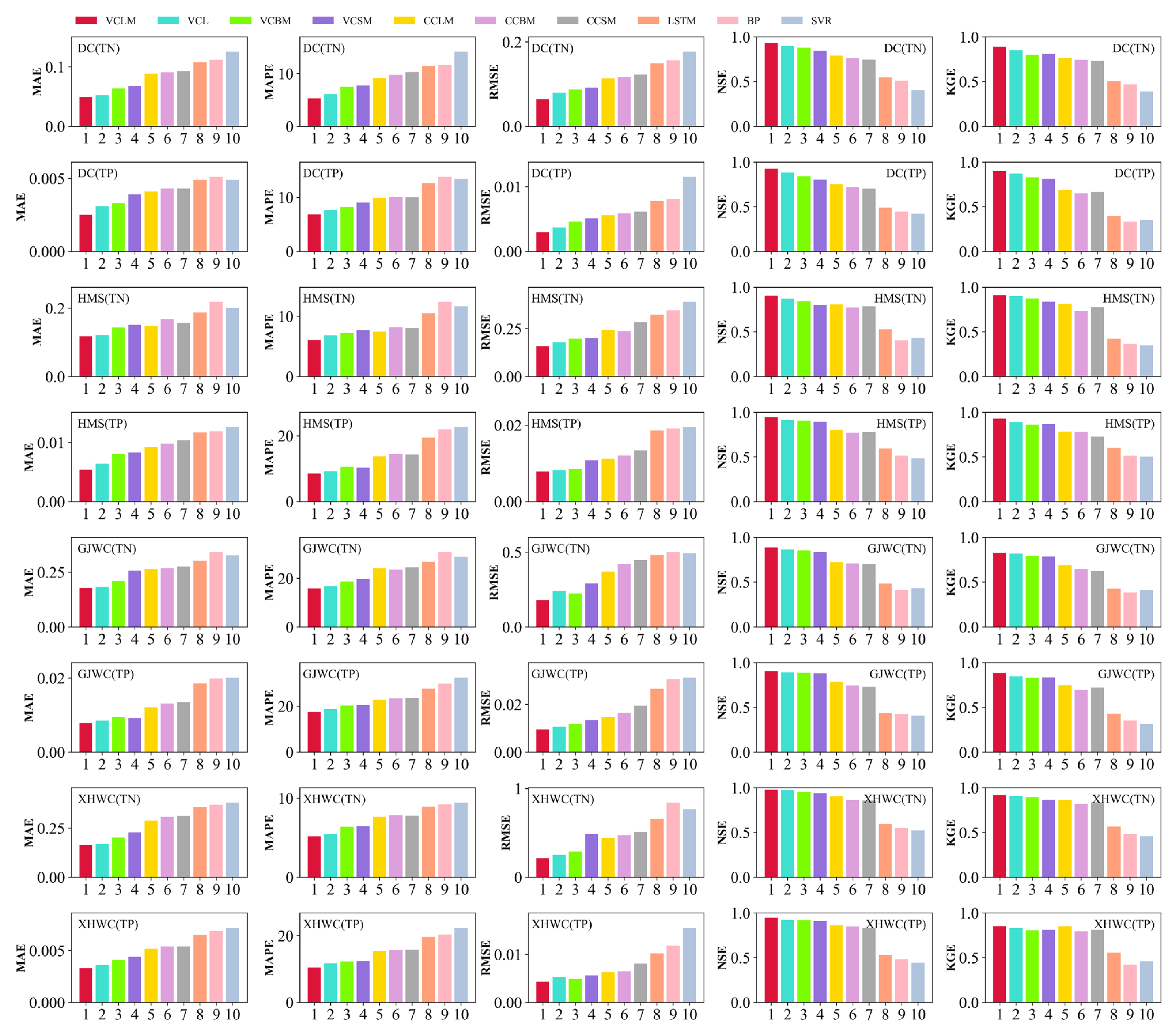
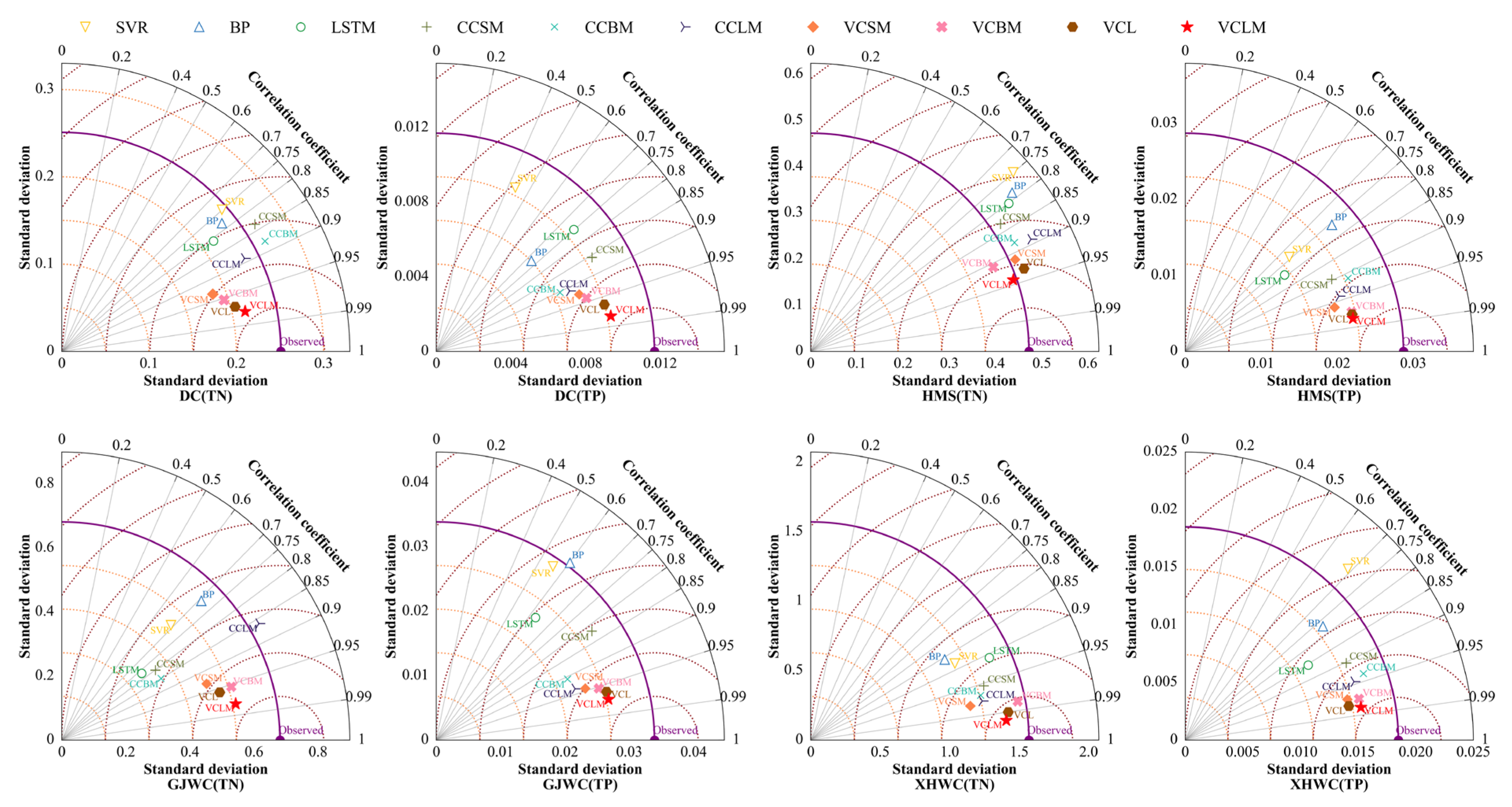
4.4.4. Water Quality Prediction Performance in Different Stations

To determine the influence of TN and TP characteristics of different stations on the prediction model, the prediction performance of the proposed VCLM model at different stations was compared further.

In terms of TN, the VCLM model achieved relatively good prediction performance at XHWC station (NSE = 0.9510 and KGE = 0.9187) and relatively poor prediction performance at GJWC station (NSE = 0.8864 and KGE = 0.8266). In terms of TP, the VCLM model achieved a relatively good prediction performance at the HMS station (NSE = 0.9485 and a KGE = 0.9275) and relatively poor prediction performance at the GJWC station (NSE = 0.9058 and KGE = 0.8536). The prediction performance of the same model on different data shows relatively large differences. This reflects that the TN and TP data fluctuations of HMS and XHWC are the most regular and easiest to predict. Intuitively, Figure 2 shows that the TN and TP data of HMS and XHWC have relatively similar volatility, and most of them show relatively stable volatility. However, whether it is TN or TP, the prediction effect in GJWC is relatively poor, indicating that the TN and TP data of GJWC are more complicated and have more uncertain factors. Figure 2 also shows that the TN and TP data of the GJWC station have large volatility and many mutation points, and these factors affect the prediction performance of the model. However, the NSE and KGE of the VCLM model on all data are greater than or equal to 0.8864 and 0.8266, respectively, thus achieving acceptable predictions.

5. Discussion

5.1. Rationality of Hindcasting and Forecasting Experiments

We further designed hindcasting and forecasting experiments using three decomposition methods, CEEMDAN, and VMD. Among them, the decomposed IMFs of each decomposition method are directly predicted and reconstructed using LSTM to obtain the final prediction results, and the hyperparameters of LSTM are calibrated using CSSA. In the hindcasting experiments, the original time series are directly decomposed into multiple IMFs before dividing the calibration and test sets, while the forecasting experiments are performed in the way proposed in Section 3.6. Finally, the experimental results obtained by applying the TN data from the DC station are presented in

Table 7. Hindcasting and forecasting experiments based on TN data from the DC station.

Item	Hindcast		Forecast
	CEEMDAN-LSTM	VMD-LSTM	CEEMDAN-LSTM	VMD-LSTM
MAE	0.0327	0.0285	0.0895	0.0523
MAPE	3.64%	3.16%	9.24%	6.15%
RMSE	0.0289	0.0157	0.1012	0.0795
NSE	0.9844	0.9987	0.7841	0.9015
KGE	0.9745	0.9824	0.7529	0.8509

.

As observed from Table 7, the results of both CEEMDAN and VMD show better performance for the hindcasting experiments compared to the forecasting experiments. In particular, the NSE and KGE of the model in the hindcasting experiment have reached more than 0.97, indicating that the predicted results of the model are essentially coincident with the actual results. This result is ideal, but it has to be noted that a prerequisite to be satisfied by the hindcasting experiment is that future data are known, which can be satisfied when we use historical data to perform simulations. This assumption is impractical from a practical application point of view, as we cannot decompose all data before dividing the calibration and test sets. In contrast, the method used by us is consistent with practical applications. By prioritizing the calibration and test sets and then decomposing them, the models are trained without using future information. Each model in the forecasting experiment does not perform as well as the hindcasting experiment, but it provides a solution to the problem of using future information and can be used for practical prediction.

5.2. Adaptive VMD Decomposition Enhances the Model Performance

Water quality parameter data can be regarded as a nonlinear and non-stationary signal sequence mixed with noise. In direct prediction, the noise part will affect the training of the model. Therefore, the data preprocessing method based on the decomposition method can separate the noise and decompose multiple more stable sub-sequences better. Forecasting for stationary subsequences can improve the accuracy of the model significantly. In many signal decomposition methods, wavelet decomposition has a wide range of applications, but the choice of wavelet base has a significant impact on the decomposition result. Thus, selecting a suitable wavelet base is necessary to achieve a better denoising effect.

To improve the wavelet decomposition technology, Huang et al. [71] developed a new adaptive signal decomposition method EMD. This method can adaptively decompose the original signal, but it has some problems, such as modal aliasing and endpoint effect. Wu and Huang [72] developed a new method EEMD, which is a substantial improvement of EMD. This method introduces Gaussian white noise to suppress modal aliasing to a certain extent, but the white noise amplitude and the number of iterations depend on human experience settings. The problem of mode aliasing cannot be overcome when the value is not properly set. Although increasing the number of ensemble averaging can reduce the reconstruction error, it also increases the computational cost, and the ensemble averaging of limited times cannot completely eliminate white noise.

To solve the problems of EEMD, Torres et al. [73] proposed CEEMDAN. This method adds positive and negative paired auxiliary white noises to the original signal, which can cancel each other during ensemble averaging, thereby overcoming the problems of large reconstruction errors and poor decomposition completeness of EEMD. At the same time, the calculation cost is greatly reduced. Recently, Dragomiretskiy and Zosso [51] proposed a new adaptive and non-recursive signal decomposition method VMD, which aimed to transfer the acquisition of the signal components to a variational framework. The decomposition of the original signal is then realized by constructing and solving constrained variational problems. However, the number of decomposed subsequences of this method needs to be determined manually. To adaptively determine the number of decompositions, this paper uses a threshold based on PE to set the number of decompositions.

This paper compares the prediction performance of the three standalone models, three hybrid models based on CEEMDAN decomposition, and three hybrid models based on VMD decomposition. The prediction performance of these models utilizes Taylor diagrams (Table 6; Figure 11). The Taylor diagram is mainly used to check the accuracy of the experimental model. It uses different points in the polar coordinates to study the difference between the observed and estimated values [74]. Figure 11 shows that the prediction result of the VCLM model has the highest correlation coefficient with the observed value and has the lowest RMSE. At the same time, combining the results of each station, VCLM, VCBM, and VCSM have higher correlation coefficients and smaller RMSE than CCLM, CCBM, and CCSM. Compared to the direct prediction model, the decomposition prediction model has a higher correlation coefficient and a smaller RMSE. The results show that the method of decomposing the original time series and predicting the sub-sequences can indeed improve the performance of the model effectively. Compared with CEEMDAN, VMD has a better decomposition effect and can extract sequence information more effectively.

5.3. LSTM Guarantees the Hybrid Model Performance

With the help of decomposition technology, LSTM-based models are better than BP-based and SVR-based models. The concentrations of TN and TP are affected by historical concentrations and reflected on various time scales. The modal components obtained by decomposition preprocessing have strong dynamic regularity and obvious time characteristics. Compared with other machine learning and neural network models, LSTM can save and retrieve input values and gradients as needed. Therefore, LSTM can extract the dynamic characteristics of TN and TP sequences.

Sarkar and De Bruyn [75] introduced LSTM to mine and predict raw data, beating 269 manual models that used other features and modeling methods. As a deep learning technology, LSTM has a multilevel representation generated by a nonlinear transformation at each level, which can be adjusted and readjusted to the characteristics represented in the computing layer based on the previous representation [76]. The algorithm used by LSTM allows it to learn and extract related advanced complex abstractions from complex datasets automatically [77]. Therefore, by using LSTM as a predictor, the capture of the linear and complex nonlinear relationship of time series is optimized to produce better prediction results.

5.4. Spatial Difference of VCLM Model Performance

The VCLM model used in this study has different prediction results for the TN and TP data of each station. VCLM has a better prediction effect on the TN data of XHWC and TP data of HMS but has a poor prediction effect on TN and TP data of GJWC. This finding may be due to extreme changes in the environment near the station during the monitoring period, resulting in a sharp increase in the concentrations of both nitrogen and phosphorus. These phenomena are manifested in the data because of sudden changes that result in uneven data distribution, which in turn makes it difficult for the predictive model to learn the rules and hidden information of the data. Due to the complexity of water quality prediction, obvious spatial differences are observed in the prediction accuracy of the VCLM model in areas with different pollutant evolution rules. Furthermore, the concentrations of TN and TP are significantly related to many human factors (e.g., agricultural fertilizers, industrial wastewater, and urban sewage). As noted by Li, et al. [48], more than 65% of the nutrient load in Poyang Lake comes from five major tributaries, and according to Figure 1, it can be seen that GJWC is close to two major tributaries (Xiuhe and Ganjiang), especially, Ganjiang is the largest tributary of Poyang Lake, with the transport in the two major tributaries, the nutrient concentration near the GJWC site fluctuates dramatically, which will lead to a decrease in model performance for short-term prediction of this site. In contrast, HMS is located at the mouth of Poyang Lake, which is less influenced by nutrients from the five major tributaries and more influenced by the nutrient concentration changes caused by the backflow of water from Yangtze River into the lake. According to our field investigation, there are a lot of sand mining boats in the middle of the lake not far from DC from July to March, and sand mining causes lake water turbidity to increase, and then it affects the nearby water’s quality.

For the pollutant sources with certain regularity or periodicity, this will help the model to predict the future water quality; thus, more data and information with direct or indirect influence on the water quality of Poyang Lake are introduced, which will help to further improve the robustness of the model. In addition, for different geographical locations, it may be more reliable to construct models based on actual pollutant sources. Furthermore, the influence of the Yangtze River on the water levels in the lake area is also a factor that cannot be ignored, and data from the hydrological monitoring stations of the mainstream of Yangtze River and the flow data from the Three Gorges Dam can be further introduced, which will help improve the interpretability of the model. However, the VCLM model varies from station to station, but the overall performance is satisfactory enough to predict the actual water’s quality accurately, which will also help to further identify pollution sources and water quality management.

6. Conclusions

A hybrid prediction model called VMD-CSSA-LSTM-MLR (VCLM) was proposed to improve the prediction accuracy of surface water quality parameters, which are highly nonlinear and nonstationary. To verify the effect of the VCLM model, the data of four online surface water quality monitoring stations in Poyang Lake were taken as examples and compared with three standalone models and six hybrid prediction models. Compared with SSA, GA, and PSO algorithms, the improved SSA algorithm called CSSA has better optimization performance. Compared to traditional BP and SVR algorithms, LSTM can capture long-term correlations of the time series well, has strong predictive ability for nonlinear time series, and can improve the reliability of water quality parameter prediction. For the different frequency characteristics of the sub-sequences decomposed by VMD, the high-frequency part is predicted by CSSA-LSTM, and the low-frequency part is predicted by MLR, which can improve the performance of the model effectively. The standalone prediction models were compared with the hybrid prediction models based on the VMD or CEEMDAN method. The prediction method after the time series can improve the prediction accuracy of the model. Furthermore, compared to CEEMDAN, the VMD method can separate the original water quality parameter time series, extract internal features effectively, and accurately describe the stationarity of the time series. The adaptive VMD method based on PE has the advantages of reducing pseudo-components effectively, avoiding modal aliasing, and improving noise robustness. By applying the ten aforementioned models to the data of four online surface water quality monitoring stations in Poyang Lake, combined with five evaluation indicators, the results show that VCLM has the best predictive effect, the best model performance, and the highest degree-of-fit to the observed value.

Although the advantages and feasibility of the proposed hybrid forecasting model based on the VMD method have been verified by actual data, some potential problems and research directions are still needed to be studied. First of all, the proposed method has large differences in the prediction performance on the data sets of different sites, and the differences in the evolution of pollutants in various regions lead to spatial differences in model performance. Therefore, in future research, we can try to add real-time updated data to better model nitrogen and phosphorus to continuously improve the accuracy of our models. Second, when extreme events, such as urban and industrial wastewater discharge, occur, models based on historical data cannot reflect the sharp increase in concentration. Therefore, in future research, we can try to introduce extreme events as influencing factors in the model to improve the performance of the model. Finally, the concentration of total nitrogen and total phosphorus will also be periodically affected by human factors, such as annual crop fertilization and occasional sand mining. Thus, including changing nitrogen and phosphorus trends in forecasting models on either a monthly or quarterly basis can further improve modeling accuracy.

References

1. Baek, S.S.; Pyo, J.; Chun, J.A. Prediction of Water Level and Water Quality Using a CNN-LSTM Combined Deep Learning Approach. Water 2020, 12, 3399. [Google Scholar] [CrossRef]
2. United States Environmental Protection Agency. Available online: https://www.epa.gov/caddis-vol2/caddis-volume-2-sources-stressors-responses-nutrients (accessed on 3 March 2022).
3. Amano, Y.; Machida, M.; Tatsumoto, H.; George, D.; Berk, S.; Taki, K. Prediction of Microcystis Blooms Based on TN:TP Ratio and Lake Origin. Sci. World J. 2008, 8, 558–572. [Google Scholar] [CrossRef] [PubMed] [Green Version]
4. Huo, S.; He, Z.; Su, J.; Xi, B.; Zhu, C. Using Artificial Neural Network Models for Eutrophication Prediction. Procedia Environ. Sci. 2013, 18, 310–316. [Google Scholar] [CrossRef] [Green Version]
5. Portielje, R.; Molen, D. Relationships between eutrophication variables: From nutrient loading to transparency. In Shallow Lakes ’98; Springer: Dordrecht, The Netherlands, 1999; Volume 143, pp. 375–387. [Google Scholar] [CrossRef]
6. Rao, K.; Zhang, X.; Wang, M.; Liu, J.; Guo, W.; Huang, W.; Xu, J. The relative importance of environmental factors in predicting phytoplankton shifting and cyanobacteria abundance in regulated shallow lakes. Environ. Pollut. 2021, 286, 117555. [Google Scholar] [CrossRef]
7. Hatvani, I.G.; Kovacs, J.; Markus, L.; Clement, A.; Hoffmann, R.; Korponai, J. Assessing the relationship of background factors governing the water quality of an agricultural watershed with changes in catchment property (W-Hungary). J. Hydrol. 2015, 521, 460–469. [Google Scholar] [CrossRef]
8. Kosten, S.; Huszar, V.L.M.; Mazzeo, N.; Scheffer, M.; da Sternberg, L.S.L.; Jeppesen, E. Lake and watershed characteristics rather than climate influence nutrient limitation in shallow lakes. Ecol. Appl. 2009, 19, 1791–1804. [Google Scholar] [CrossRef]
9. Varol, M. Temporal and spatial dynamics of nitrogen and phosphorus in surface water and sediments of a transboundary river located in the semi-arid region of Turkey. Catena 2013, 100, 1–9. [Google Scholar] [CrossRef]
10. Sinshaw, T.A. Artificial Neural Network for Prediction of Total Nitrogen and Phosphorus in US Lakes. J. Environ. Eng. 2019, 145, 04019032. [Google Scholar] [CrossRef]
11. Song, C.; Chen, X. Performance Comparison of Machine Learning Models for Annual Precipitation Prediction Using Different Decomposition Methods. Remote Sens. 2021, 13, 1018. [Google Scholar] [CrossRef]
12. Arnold, J.G.; Moriasi, D.N.; Gassman, P.W.; Abbaspour, K.C.; White, M.J.; Srinivasan, R.; Santhi, C.; Harmel, R.D.; Van Griensven, A.; Van Liew, M.W.; et al. SWAT: Model Use, Calibration, and Validation. Trans. ASABE 2012, 55, 1491–1508. [Google Scholar] [CrossRef]
13. Huber, W.C.; Heaney, J.P.; Cunningham, B.A.; Barnwell, T.O. Storm Water Management Model (SWMM) Bibliography; Environmental Research Laboratory, Office of Research and Development, US Environmental Protection Agency: Washington, DC, USA, 1985.
14. Lin, S.; Jing, C.; Chaplot, V.; Yu, X.; Zhang, Z.; Moore, N.; Wu, J. Effect of DEM resolution on SWAT outputs of runoff, sediment and nutrients. Hydrol. Earth Syst. Sci. Discuss. 2010, 7, 4411–4435. [Google Scholar] [CrossRef]
15. Baek, S.S.; Ligaray, M.; Pyo, J.; Park, J.P.; Kang, J.H.; Pachepsky, Y.; Chun, J.A.; Cho, K.H. A novel water quality module of the SWMM model for assessing low impact development (LID) in urban watersheds. J. Hydrol. 2020, 586, 124886. [Google Scholar] [CrossRef]
16. Choubin, B.; Borji, M.; Hosseini, F.S.; Mosavi, A.; Dineva, A.A. Mass wasting susceptibility assessment of snow avalanches using machine learning models. Sci. Rep. 2020, 10, 18363. [Google Scholar] [CrossRef] [PubMed]
17. Choubin, B.; Hosseini, F.S.; Fried, Z.; Mosavi, A. Application of Bayesian Regularized Neural Networks for Groundwater Level Modeling. In Proceedings of the 2020 IEEE 3rd International Conference and Workshop in Óbuda on Electrical and Power Engineering (CANDO-EPE), Budapest, Hungary, 18–19 November 2020; pp. 209–212. [Google Scholar] [CrossRef]
18. Li, X.; Yan, D.; Wang, K.; Weng, B.; Qin, T.; Liu, S. Flood Risk Assessment of Global Watersheds Based on Multiple Machine Learning Models. Water 2019, 11, 1654. [Google Scholar] [CrossRef] [Green Version]
19. Mosavi, A.; Golshan, M.; Janizadeh, S.; Choubin, B.; Melesse, A.M.; Dineva, A.A. Ensemble models of GLM, FDA, MARS, and RF for flood and erosion susceptibility mapping: A priority assessment of sub-basins. Geocarto Int. 2020, 35, 1–20. [Google Scholar] [CrossRef]
20. Chen, K.; Chen, H.; Zhou, C.; Huang, Y.; Qi, X.; Shen, R.; Liu, F.; Zuo, M.; Zou, X.; Wang, J.; et al. Comparative analysis of surface water quality prediction performance and identification of key water parameters using different machine learning models based on big data. Water Res. 2020, 171, 115454. [Google Scholar] [CrossRef]
21. Fang, X.; Li, X.; Zhang, Y.; Zhao, Y.; Qian, J.; Hao, C.; Zhou, J.; Wu, Y. Random forest-based understanding and predicting of the impacts of anthropogenic nutrient inputs on the water quality of a tropical lagoon. Environ. Res. Lett. 2021, 16, 055003. [Google Scholar] [CrossRef]
22. Liu, S.; Tai, H.; Ding, Q.; Li, D.; Xu, L.; Wei, Y. A hybrid approach of support vector regression with genetic algorithm optimization for aquaculture water quality prediction. Math. Comput. Model. 2013, 58, 458–465. [Google Scholar] [CrossRef]
23. Mahmoudi, N.; Orouji, H.; Fallah-Mehdipour, E. Integration of Shuffled Frog Leaping Algorithm and Support Vector Regression for Prediction of Water Quality Parameters. Water Resour. Manag. 2016, 30, 2195–2211. [Google Scholar] [CrossRef]
24. Jadhav, M.S.; Khare, K.C.; Warke, A.S. Water Quality Prediction of Gangapur Reservoir (India) Using LS-SVM and Genetic Programming. Lakes Reserv. Sci. Policy Manag. Sustain. Use 2015, 20, 275–284. [Google Scholar] [CrossRef]
25. Xiang, Y.; Jiang, L. Water Quality Prediction Using LS-SVM and Particle Swarm Optimization. In Proceedings of the 2009 Second International Workshop on Knowledge Discovery and Data Mining, Moscow, Russia, 23–25 January 2009; pp. 900–904. [Google Scholar] [CrossRef]
26. Anmala, J.; Turuganti, V. Comparison of the performance of decision tree (DT) algorithms and extreme learning machine (ELM) model in the prediction of water quality of the Upper Green River watershed. Water Environ. Res. 2021, 93, 2360–2373. [Google Scholar] [CrossRef] [PubMed]
27. Yu, T.; Bai, Y. Comparative Study of Optimization Intelligent Models in Wastewater Quality Prediction. In Proceedings of the 2018 International Conference on Sensing, Diagnostics, Prognostics, and Control (SDPC), Xi’an, China, 15–17 August 2018; pp. 221–225. [Google Scholar] [CrossRef]
28. Azad, A.; Karami, H.; Farzin, S.; Saeedian, A.; Kashi, H.; Sayyahi, F. Prediction of Water Quality Parameters Using ANFIS Optimized by Intelligence Algorithms (Case Study: Gorganrood River). KSCE J. Civ. Eng. 2018, 22, 2206–2213. [Google Scholar] [CrossRef]
29. Fu, Z.; Cheng, J.; Yang, M.; Batista, J.; Jiang, Y. Wastewater discharge quality prediction using stratified sampling and wavelet de-noising ANFIS model. Comput. Electr. Eng. 2020, 85, 106701. [Google Scholar] [CrossRef]
30. Jin, T.; Cai, S.; Jiang, D.; Liu, J. A data-driven model for real-time water quality prediction and early warning by an integration method. Environ. Sci. Pollut. Res. 2019, 26, 30374–30385. [Google Scholar] [CrossRef] [PubMed]
31. Zhang, Z.; Wang, X.; Ou, Y. Water Simulation Method Based on BPNN Response and Analytic Geometry. Procedia Environ. Sci. 2010, 2, 446–453. [Google Scholar] [CrossRef] [Green Version]
32. Han, H.G.; Chen, Q.L.; Qiao, J.F. An efficient self-organizing RBF neural network for water quality prediction. Neural Netw. 2011, 24, 717–725. [Google Scholar] [CrossRef]
33. Weihui, D.; Guoyin, W.; Xuerui, Z.; Yishuai, G.; Guangdi, L. Water quality prediction based on a novel hybrid model of ARIMA and RBF neural network. In Proceedings of the 2014 IEEE 3rd International Conference on Cloud Computing and Intelligence Systems, 27–29 November 2014; pp. 33–40. [Google Scholar] [CrossRef]
34. Wang, X.; Wang, Y.; Yuan, P.; Wang, L.; Cheng, D. An adaptive daily runoff forecast model using VMD-LSTM-PSO hybrid approach. Hydrol. Sci. J. 2021, 66, 1488–1502. [Google Scholar] [CrossRef]
35. Hochreiter, S.; Schmidhuber, J. Long Short-Term Memory. Neural Comput. 1997, 9, 1735–1780. [Google Scholar] [CrossRef]
36. Liu, P.; Wang, J.; Sangaiah, A.K.; Xie, Y.; Yin, X. Analysis and Prediction of Water Quality Using LSTM Deep Neural Networks in IoT Environment. Sustainability 2019, 11, 2058. [Google Scholar] [CrossRef] [Green Version]
37. Lu, H.; Ma, X. Hybrid decision tree-based machine learning models for short-term water quality prediction. Chemosphere 2020, 249, 126169. [Google Scholar] [CrossRef]
38. Wang, Y.; Zhou, J.; Chen, K.; Wang, Y.; Liu, L. Water quality prediction method based on LSTM neural network. In Proceedings of the 2017 12th International Conference on Intelligent Systems and Knowledge Engineering (ISKE), Nanjing, China, 24–26 November 2017; pp. 1–5. [Google Scholar] [CrossRef]
39. Bai, Y.; Liu, M.D.; Ding, L.; Ma, Y.J. Double-layer staged training echo-state networks for wind speed prediction using variational mode decomposition. Appl. Energy 2021, 301, 117461. [Google Scholar] [CrossRef]
40. Zhang, J.; Qiu, H.; Li, X.; Niu, J.; Nevers, M.B.; Hu, X.; Phanikumar, M.S. Real-Time Nowcasting of Microbiological Water Quality at Recreational Beaches: A Wavelet and Artificial Neural Network-Based Hybrid Modeling Approach. Environ. Sci. Technol. 2018, 52, 8446–8455. [Google Scholar] [CrossRef] [PubMed]
41. Liu, S.; Xu, L.; Li, D. Multi-scale prediction of water temperature using empirical mode decomposition with back-propagation neural networks. Comput. Electr. Eng. 2016, 49, 1–8. [Google Scholar] [CrossRef]
42. Li, C.; Li, Z.; Wu, J.; Zhu, L.; Yue, J. A hybrid model for dissolved oxygen prediction in aquaculture based on multi-scale features. Inf. Process. Agric. 2018, 5, 11–20. [Google Scholar] [CrossRef]
43. Zounemat-Kermani, M.; Seo, Y.; Kim, S.; Ghorbani, M.; Samadianfard, S.; Naghshara, S.; Kim, N.W.; Singh, V.P. Can Decomposition Approaches Always Enhance Soft Computing Models? Predicting the Dissolved Oxygen Concentration in the St. Johns River, Florida. Appl. Sci. 2019, 9, 2534. [Google Scholar] [CrossRef] [Green Version]
44. Song, C.; Yao, L.; Hua, C.; Ni, Q. A water quality prediction model based on variational mode decomposition and the least squares support vector machine optimized by the sparrow search algorithm (VMD-SSA-LSSVM) of the Yangtze River, China. Environ. Monit. Assess. 2021, 193, 363. [Google Scholar] [CrossRef]
45. Huang, J.; Huang, Y.; Hassan, S.G.; Xu, L.; Liu, S. Dissolved oxygen content interval prediction based on auto regression recurrent neural network. J. Ambient. Intell. Humaniz. Comput. 2021, 12, 1–10. [Google Scholar] [CrossRef]
46. Fijani, E.; Barzegar, R.; Deo, R.; Tziritis, E.; Skordas, K. Design and implementation of a hybrid model based on two-layer decomposition method coupled with extreme learning machines to support real-time environmental monitoring of water quality parameters. Sci. Total Environ. 2019, 648, 839–853. [Google Scholar] [CrossRef]
47. Dong, L.; Zhang, J. Predicting polycyclic aromatic hydrocarbons in surface water by a multiscale feature extraction-based deep learning approach. Sci. Total Environ. 2021, 799, 149509. [Google Scholar] [CrossRef]
48. Li, B.; Yang, G.; Wan, R. Multidecadal water quality deterioration in the largest freshwater lake in China (Poyang Lake): Implications on eutrophication management. Environ. Pollut. 2020, 260, 114033. [Google Scholar] [CrossRef]
49. Tang, X.; Li, H.; Xu, X.; Yang, G.; Liu, G.; Li, X.; Chen, D. Changing land use and its impact on the habitat suitability for wintering Anseriformes in China’s Poyang Lake region. Sci. Total Environ. 2016, 557, 296–306. [Google Scholar] [CrossRef] [PubMed]
50. Wantzen, K.M.; Rothhaupt, K.O.; Mörtl, M.; Cantonati, M.; Tóth, L.G.; Fischer, P. Ecological effects of water-level fluctuations in lakes: An urgent issue. In Ecological Effects of Water-Level Fluctuations in Lakes; Springer: Berlin/Heidelberg, Germany, 2008; Volume 204, pp. 1–4. [Google Scholar] [CrossRef] [Green Version]
51. Dragomiretskiy, K.; Zosso, D. Variational Mode Decomposition. IEEE Trans. Signal Process. 2014, 62, 531–544. [Google Scholar] [CrossRef]
52. Bandt, C.; Pompe, B. Permutation Entropy: A Natural Complexity Measure for Time Series. Phys. Rev. Lett. 2002, 88, 174102. [Google Scholar] [CrossRef] [PubMed]
53. Stosic, T.; Stosic, B.; Singh, V.P. Optimizing streamflow monitoring networks using joint permutation entropy. J. Hydrol. 2017, 552, 306–312. [Google Scholar] [CrossRef]
54. Gao, S.; Huang, Y.; Zhang, S.; Han, J.; Wang, G.; Zhang, M.; Lin, Q. Short-term runoff prediction with GRU and LSTM networks without requiring time step optimization during sample generation. J. Hydrol. 2020, 589, 125188. [Google Scholar] [CrossRef]
55. Xue, J.; Shen, B. A novel swarm intelligence optimization approach: Sparrow search algorithm. Syst. Sci. Control. Eng. 2020, 8, 22–34. [Google Scholar] [CrossRef]
56. Wang, P.; Zhang, Y.; Yang, H. Research on Economic Optimization of Microgrid Cluster Based on Chaos Sparrow Search Algorithm. Comput. Intell. Neurosci. 2021, 2021, 5556780. [Google Scholar] [CrossRef]
57. Liu, L.; Sun, S.Z.; Yu, H.; Yue, X.; Zhang, D. A modified Fuzzy C-Means (FCM) Clustering algorithm and its application on carbonate fluid identification. J. Appl. Geophys. 2016, 129, 28–35. [Google Scholar] [CrossRef]
58. Rudolph, G. Local convergence rates of simple evolutionary algorithms with Cauchy mutations. IEEE Trans. Evol. Comput. 1997, 1, 249–258. [Google Scholar] [CrossRef]
59. Li, J.; Deng, D.; Zhao, J.; Cai, D.; Hu, W.; Zhang, M.; Huang, Q. A Novel Hybrid Short-Term Load Forecasting Method of Smart Grid Using MLR and LSTM Neural Network. IEEE Trans. Ind. Inform. 2021, 17, 2443–2452. [Google Scholar] [CrossRef]
60. Zhang, X.; Peng, Y.; Zhang, C.; Wang, B. Are hybrid models integrated with data preprocessing techniques suitable for monthly streamflow forecasting? Some experiment evidences. J. Hydrol. 2015, 530, 137–152. [Google Scholar] [CrossRef]
61. Zuo, G.; Luo, J.; Wang, N.; Lian, Y.; He, X. Two-stage variational mode decomposition and support vector regression for streamflow forecasting. Hydrol. Earth Syst. Sci. 2020, 24, 5491–5518. [Google Scholar] [CrossRef]
62. Pool, S.; Vis, M.; Seibert, J. Evaluating model performance: Towards a non-parametric variant of the Kling-Gupta efficiency. Hydrol. Sci. J. 2018, 63, 1941–1953. [Google Scholar] [CrossRef]
63. He, X.; Luo, J.; Li, P.; Zuo, G.; Xie, J. A Hybrid Model Based on Variational Mode Decomposition and Gradient Boosting Regression Tree for Monthly Runoff Forecasting. Water Resour. Manag. 2020, 34, 865–884. [Google Scholar] [CrossRef]
64. Feng, Z.; Niu, W.; Tang, Z.; Jiang, Z.; Xu, Y.; Liu, Y.; Zhang, H. Monthly runoff time series prediction by variational mode decomposition and support vector machine based on quantum-behaved particle swarm optimization. J. Hydrol. 2020, 583, 124627. [Google Scholar] [CrossRef]
65. Huang, S.; Chang, J.; Huang, Q.; Chen, Y. Monthly streamflow prediction using modified EMD-based support vector machine. J. Hydrol. 2014, 511, 764–775. [Google Scholar] [CrossRef]
66. Wang, J.; Wang, X.; Lei, X.; Wang, H.; Zhang, X.; You, J.; Tan, Q.; Liu, X. Teleconnection analysis of monthly streamflow using ensemble empirical mode decomposition. J. Hydrol. 2019, 582, 124411. [Google Scholar] [CrossRef]
67. Mirjalili, S.; Mirjalili, S.M.; Lewis, A. Grey wolf optimizer. Adv. Eng. Softw. 2014, 69, 46–61. [Google Scholar] [CrossRef] [Green Version]
68. Kennedy, J.; Eberhart, R. Particle swarm optimization. In Proceedings of the ICNN’95-International Conference on Neural Networks, Perth, WA, Australia, 27 November–1 December 1995; Volume 4, pp. 1942–1948. [Google Scholar] [CrossRef]
69. Rashedi, E.; Nezamabadi-Pour, H.; Saryazdi, S. GSA: A gravitational search algorithm. Inf. Sci. 2009, 179, 2232–2248. [Google Scholar] [CrossRef]
70. Yang, X.S. Flower pollination algorithm for global optimization. In Proceedings of the International Conference on Unconventional Computing and Natural Computation, Orléan, France, 3–7 September 2012; pp. 240–249. [Google Scholar] [CrossRef] [Green Version]
71. Huang, N.E.; Shen, Z.; Long, S.R.; Wu, M.C.; Shih, H.H.; Zheng, Q.; Yen, N.C.; Tung, C.C.; Liu, H. The empirical mode decomposition and the Hilbert spectrum for nonlinear and non-stationary time series analysis. Proc. R. Soc. Lond. Ser. A Math. Phys. Eng. Sci. 1998, 454, 903–995. [Google Scholar] [CrossRef]
72. Wu, Z.; Huang, N.E. Ensemble empirical mode decomposition: A noise-assisted data analysis method. Adv. Adapt. Data Anal. 2009, 1, 1–41. [Google Scholar] [CrossRef]
73. Torres, M.E.; Colominas, M.A.; Schlotthauer, G.; Flandrin, P. A complete ensemble empirical mode decomposition with adaptive noise. In Proceedings of the 2011 IEEE International Conference on Acoustics, Speech and Signal Processing (ICASSP), Prague, Czech Republic, 22–27 May 2011; pp. 4144–4147. [Google Scholar] [CrossRef]
74. Kargar, K.; Samadianfard, S.; Parsa, J.; Nabipour, N.; Shamshirband, S.; Mosavi, A.; Chau, K.W. Estimating longitudinal dispersion coefficient in natural streams using empirical models and machine learning algorithms. Eng. Appl. Comput. Fluid Mech. 2020, 14, 311–322. [Google Scholar] [CrossRef]
75. Sarkar, M.; De Bruyn, A. LSTM Response Models for Direct Marketing Analytics: Replacing Feature Engineering with Deep Learning. J. Interact. Mark. 2021, 53, 80–95. [Google Scholar] [CrossRef]
76. Reddy, B.K.; Delen, D. Predicting hospital readmission for lupus patients: An RNN-LSTM-based deep-learning methodology. Comput. Biol. Med. 2018, 101, 199–209. [Google Scholar] [CrossRef]
77. LeCun, Y.; Bengio, Y.; Hinton, G. Deep learning. Nature 2015, 521, 436–444. [Google Scholar] [CrossRef] [PubMed]
Figure 1. Study sites in the Poyang Lake.
Water 14 01643 g001
Figure 2. Observed data of TN and TP at (a) DC, (b) HMS, (c) GJWC, and (d) XHWC.
Water 14 01643 g002
Figure 3. Long Short-Term Memory unit structure diagram.
Water 14 01643 g003
Figure 4. Flow chart of the VCLM prediction structure.
Water 14 01643 g004
Figure 5. Decomposed sub-series results of TN using VMD at the DC station: (a) the decomposition sequence waveform and (b) the frequency spectrum representation.
Water 14 01643 g005
Figure 6. Correlation of 8 characteristic lag times of 1–15 days with (a) TN (IMF1), (b) TN (IMF2), (c) TP (IMF1), and (d) TP (IMF2) at DC station.
Water 14 01643 g006
Figure 7. PACF analysis of low-frequency (IMF1 and IMF2) components.
Water 14 01643 g007
Figure 8. Forecasted total nitrogen (TN) obtained by (a) standalone models, (b) CEEMDAN-based models, and (c) VMD-based models at the DC station.
Water 14 01643 g008
Figure 9. Forecasted total phosphorus (TP) obtained by (a) standalone, (b) CEEMDAN-based, and (c) VMD-based models at the DC station.
Water 14 01643 g009
Figure 10. Histogram of model prediction evaluation metrics.
Water 14 01643 g010
Figure 11. Taylor diagram that compares the performance of applied algorithms.
Water 14 01643 g011