
Contaminant Fate and Transport Modeling in Distribution Systems: EPANET-C


Civil and Environmental Engineering, Technion—Israel Institute of Technology, Haifa 32000, Israel
*
Author to whom correspondence should be addressed.
Water 2022, 14(10), 1665; https://0-doi-org.brum.beds.ac.uk/10.3390/w14101665
Submission received: 22 April 2022
/
Revised: 13 May 2022
/
Accepted: 19 May 2022
/
Published: 23 May 2022
(This article belongs to the Section Water Quality and Contamination)
Abstract
:Typically, computer-based tools built on mathematical models define the time-series behavior of contaminants, in dissolved or colloidal form, within the spatial boundaries of water distribution systems (WDS). EPANET-MSX has become a standard tool for WDS quality modeling due to its collaboration with EPANET. The critical challenges in applying EPANET-MSX include conceptualizing the exchanges among multiple reacting constituents within the WDS domain and developing the scientific descriptions of these exchanges. Moreover, due to its complicated user interface, the EPANET-MSX application demands programming skills from a software engineering viewpoint. The present study aims to overcome these challenges by developing a novel computer-based tool, EPANET-C. Via built-in and customizable conceptual and mathematical models’ directories, EPANET-C simplifies WDS water quality modeling for users, even those lacking programming expertise. Due to its flexibility, EPANET-C can become a de facto standard tool in WDS quality modeling study both for the industry and the academia.
1. Introduction
Water distribution systems (WDS) are interconnected assemblies of reservoirs, tanks, pipes, and hydraulic control elements and are considered as critical infrastructure of every modern community. Due to their spatial extent and accessibility, a potential contamination event in the WDS may cause acute or chlorine health impacts to numerous consumers within a brief period. Hence, they are deemed vulnerable to public health risks. The WDS contamination events may be instigated accidentally [1] or even intentionally [2,3,4]. Either way, they have severe consequences and thus remain significant potential threats concerning WDS operation.
In general, considering these apprehensions, computer-based tools adept at simulating WDS response to contamination events are perceived as pragmatic solutions to safeguarding the integrity of WDS operation [5]. These tools, built on mathematical models, define the behavior of contaminants (microbiological and/or chemical), in dissolved or colloidal form, within the spatial boundaries of WDS. More specifically, five governing mechanisms are considered significant when developing mathematical models for directing the WDS response to contamination or to contaminant behavior in WDS. They include: (1) the physical rules regulating the flow characteristics within the distribution network, (2) the rate and duration of contamination, (3) the physical, chemical, physicochemical, and biochemical mechanisms administering the contaminant’s fate within the spatial domain of the WDS, (4) the dynamics of the supply and extraction of water at the source and demand points, respectively, and (5) the network configuration.
Numerous past studies detailing several efforts to mathematically express the five governing mechanisms above and to solve the resulting equations analytically and numerically are available in the literature. Most of these studies focused solely on the fate and transport of a single contaminant, typically disinfectant chemicals such as chlorine, in distribution pipes [6,7,8,9,10,11,12,13,14,15,16]. Thus, most of the water quality models found in the literature are characterizable as ‘single species models’. Only limited studies have combined the exchanges among various abiotic and biotic reacting constituents in WDS to simulate the spatiotemporal distributions of microbiological and/or chemical water quality parameters [17,18,19,20,21,22,23,24,25,26,27,28,29,30,31,32,33]. Such models which consider the multi-species exchanges within the WDS domain are distinguishable as ‘multi-species reactive-transport (MSRT) models’.
Albeit conceptual differences exist, the fundamental challenge of appropriately addressing the complexity of WDS behavior—defined by non-linear and non-smooth head–flow–water quality governing equations bounded with a high number of constraints and decision variables—is common for both single-species and MSRT modeling. However, two challenges necessitate particular attention during MSRT modeling as compared to single-species modeling. They are: (a) the conceptualization of the exchanges among multiple abiotic and biotic reacting constituents and (b) the development of scientific descriptions of these exchanges.
Nevertheless, abstracting the multi-species exchanges within the system domain during the conceptual stage of MSRT modeling is typically viewed as a notional process whose scope is totally limited by the problem settings. Thus, the MSRT models in the literature are principally problem-specific. By this logic, they lack pertinence beyond the settings they are developed for. For instance, the MSRT model by Abhijith et al. [32] is fit to simulate the planktonic microbial regrowth dynamics in WDS. However, examining the potential for the occurrence of taste and odor (T&O) problems or investigating the formation of per- and polyfluoroalkyl substances (PFASs) in WDS is beyond its scope.
This limitation of current MSRT models raises the question, ‘can a comprehensive tool be developed?’ If such a tool could facilitate the study of the behavior of plentiful contaminants in WDS, it would arguably be an invaluable asset for examining the WDS response towards numerous contamination events. This paper attempts to answer this question by presenting a novel computer-based tool, EPANET-C, which allows for the examination of WDS response to diverse contamination events. EPANET-C is designed to function as an advanced open-source extension of EPANET [34]–EPANET-MSX [35] modeling. It uses function directories to integrate the necessary resources for implementing MSRT models via the well-established EPANET–EPANET-MSX framework [19,21,24,25,32,33].
The next section of this paper provides an inclusive description of the theory behind conceptualizing the exchanges between eleven reacting constituents, i.e., nine abiotic constituents—chlorine, total organic carbon (TOC), biodegradable dissolved organic carbon (BDOC), trihalomethanes (THMs), 2,4,6-trichlorophenol (2,4,6-TCP), 2,4,6-trichloroanisole (2,4,6-TCA), perfluorooctane amido betaine (PFOAB), perfluorooctane amido ammonium salt (PFOAAmS), and perfluorooctanoic acid (PFOA)—and two biotic constituents—planktonic and biofilm microorganisms—in WDS. Later, a brief outline of the EPANET-C function directories and its user interface is provided. Then, its application is demonstrated via two well-tested real-world WDS: the North Marin Water District WDS, USA [34] and the BWSN Network 1 [36]. The case studies established that EPANET-C offers an easy-to-use platform for analyzing WDS water quality, which otherwise needs synergistic knowledge in chemistry, biology, mathematics, and computer programming.
2. Conceptual Background
EPANET-C incorporates fifteen MSRT modules, each integrating the transport (via advection) and exchanges (physical, chemical, physicochemical, and biochemical reactions) of different combinations of the eleven reacting constituents mentioned above. The details of the MSRT modules are described in Table 1. The scientific information provided in the authors’ previous works [24,25,32,33] was studied to establish the theoretical backgrounds of these modules.
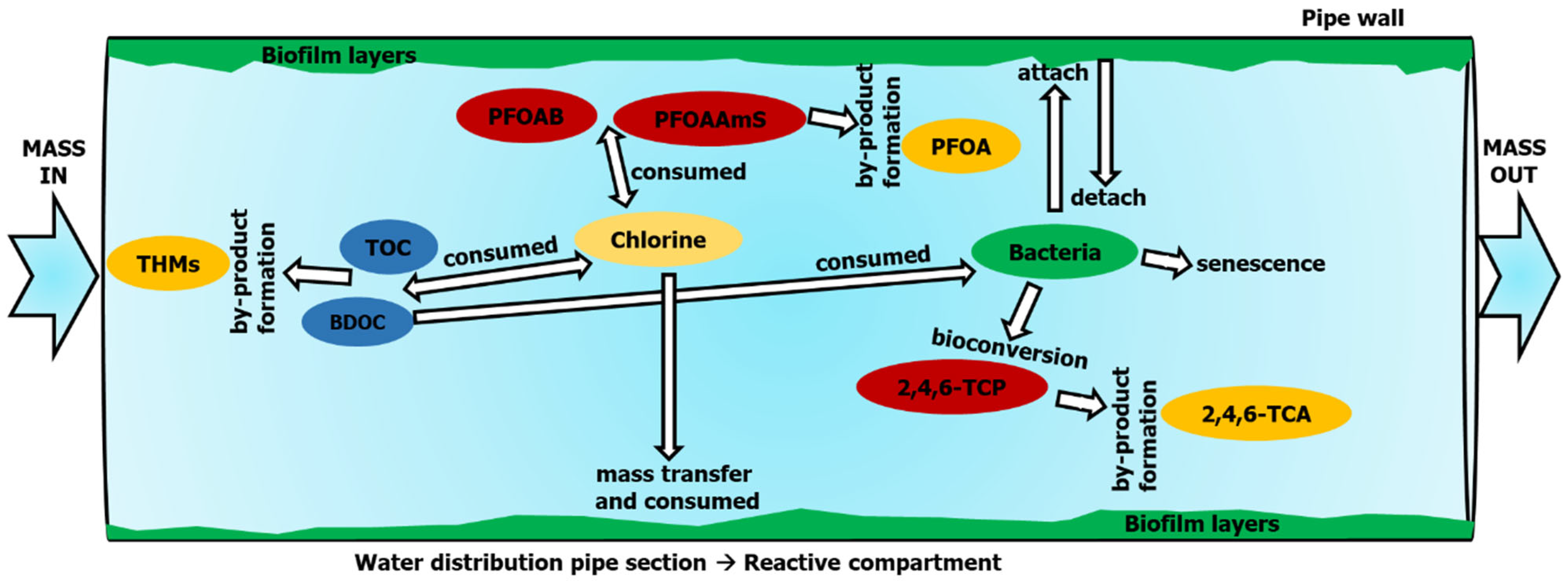
The concepts discussed by Abhijith et al. [32] were used to formulate the EPANET-C module concerning microbial regrowth and another one relating to THM formation. Similarly, the information described by Abhijith and Ostfeld in [24,33] were applied in order to develop the T&O problems formation and the PFOA formation modules separately. The microbial regrowth, THM formation, T&O problems formation, and PFOA formation modules are denoted in EPANET-C by the notations ‘1’, ‘2’, ‘3’, and ‘4’, respectively. These four modules were combined in every prospect to create the remaining eleven EPANET-C modules. As seen in Table 1, ‘12’ points were assigned to the microbial regrowth and THM formation module, which was generated by combining the distinct microbial regrowth and THM formation modules. This combined module was designed to concurrently simulate the microbiological and chemical quality variations in WDS. Equally, the notation of ‘34’ corresponds to the T&O and PFOA formation module of EPANET-C. This module can be applied to analyze the organoleptic and chemical quality variations in WDS. Likewise, the notation ‘1234’ indicates the comprehensive module of EPANET-C. This was developed for the simultaneous modeling of the microbiological, chemical, and organoleptic quality variations during WDS operation. The conceptual model graphic of the comprehensive EPANET-C module (i.e., 1234) is presented in Figure 1.
Figure 1 shows that the WDS domain (system environment) is divided into bulk and wall phases for conceptualizing the multi-species exchanges in the EPANET-C modules. The bulk phase is deemed to be the lively compartment of a distribution pipe in which the advection principally controls the transfer of reacting constituents along the water flow route. For storage tanks, the bulk phase signifies its inside space, characterizing itself as a continuously stirred tank reactor. On the contrary, the wall phase is the pseudo-stationary compartment representing the biofilm layers, which are uniformly distributed inside the pipe surface. The wall phase is limited to distribution pipes alone. It is characterized as a batch reactor with zero mass flux [26]. Out of the eleven reacting constituents, ten of them, except for biofilm microorganisms, are bulk species. This implies that these ten reacting constituents only exist in the bulk phase of the WDS domain. Biofilm microorganisms are the sole wall species, and they are only present in the wall phase of the distribution pipes.
Chlorine is assumed to be the disinfectant chemical in the EPANET-C modules, given its dominant global use. Hypochlorous acid, the weak acid formed by chlorine hydrolysis, was chosen to define the impressions of maintenance disinfectant residues in WDS. Nonetheless, provisions were made to be able to easily alter the values of the reaction rate constant that describes chlorine reactions. In this way, the adaptability to the effects of pH in chlorine hydrolysis was intrinsically incorporated into EPANET-C.
TOC was accepted as the surrogate parameter for natural organic matter (NOM) content in WDS. The biodegradable fraction of TOC, i.e., BDOC, was recognized as the substrate that the heterotrophic microorganisms could mineralize in WDS [37]. TOC only signifies the mass of the organic compounds in water. It does not characterize their specific structure or functional group effects [38]. Hence, the effects of NOM content in determining the chlorine dynamics, including functional group oxidation and electrophilic substitution by chlorine, were ignored in EPANET-C.
THMs, which account for most of the halogenated disinfection by-products (DBPs) in WDS [39] and which induce carcinogenic and reproductive risks [40], were selected as the surrogate parameter for DBPs in the delivered water. They were presumed to be formed by chlorine–TOC reactions. The involvement of microorganisms in DBP formation [29] was ignored in the MSRT modules for simplification.
2,4,6-TCA (C7H5Cl3O) is a common T&O problem-inducing contaminant in WDS [41]. Its occurrence has been reported in drinking water sources and WDS worldwide [42,43,44]. 2,4,6-TCA is reported to have a very low olfactory threshold value of about 30 ng/L [45]. In developing the MSRT modules, 2,4,6-TCP (C6H2Cl3OH)—a common environmental pollutant recurrently detected in water sources [46]—was selected as the precursor compound of 2,4,6-TCA. 2,4,6-TCA forms predominantly in WDS through the bioconversion of 2,4,6-TCP via microbial O-methylation. During this process, the planktonic microorganisms, using the chlorophenol O-methyltransferases (CPOMT) enzyme [47], transfer a methyl group from methyl donors—methanol, methylamines, and methanethiol—to the hydroxyl group of 2,4,6-TCP to produce 2,4,6-TCA [48].
PFOA (C7F15COOH) is an anionic organic PFAS that is most often reported and deliberated in the scientific literature [49] and in legal frameworks for water quality [50]. Past studies have confirmed the role of PFOAB (C15H15F15N2O3) and PFOAAmS (C14H16F15IN2O), respectively a zwitterionic and a cationic fluoroalkyl amide (FA), in directing PFOA formation [51] in the treated water and the subsequent PFAS contamination at the consumer end of chlorinated WDS [24]. Therefore, PFOA was selected as the surrogate for PFASs, and PFOAB and PFOAAmS were chosen as the precursor FA compounds to simulate PFAS formation in the MSRT modules. PFOA formation was presumed to occur under direct chlorine–PFOAB and chlorine–PFOAAmS reactions in aquatic systems [51].
The Pseudomonas bacteria strains, largely present in WDS [52,53], were selected as the surrogates for microorganisms living within the bulk and wall phase of WDS. Although microorganisms are colloidal solids, they were extrapolated as dissolved solids, purely from a mathematical modeling perspective, by representing them according to the organic carbon content of their cells. The organic carbon content of Pseudomonas bacterial cells is reported to vary between 1.04 × 10⁻⁸ and 1.40 × 10⁻⁹ mg/CFU [54,55,56]. In the MSRT modules, the organic carbon content of planktonic and biofilm microorganisms was approximated to be at 10−9 mg/CFU [28,29,31].
3. Mathematical Modelling
The kinetic relationships specified in the literature were carefully chosen in order to develop scientific descriptions of the exchanges between the eleven abiotic and biotic reacting constituents of the EPANET-C modules. A simple two-constituent second-order kinetic model [38] was used to signify the chlorine–TOC/BDOC reactions and the subsequent chlorine decay and TOC/BDOC degradation in aquatic systems (Equations (1)–(3)). The THMs formation, a by-product of chlorine–TOC reactions, was modeled with a reaction yield coefficient (Equation (4)).
where = concentration of residual chlorine (mg/L); = concentration of TOC (mg/L); = concentration of BDOC (mg/L); = concentration of THMs (µg/L); = time (h); = second-order rate constant corresponding to chlorine–TOC/BDOC reactions (L/mg/h); = yield coefficient for TOC/BDOC corresponding to chlorine–TOC/BDOC reactions (mg/mg); and = reaction yield coefficient corresponding to THM formation from organic matter (µg/mg).
The mass transfer of chlorine from the bulk to the biofilm or the pipe wall layers via molecular diffusion was presumed to occur across an imaginary boundary layer. In connection with this, the mass transfer mechanism and the chlorine consumption on the pipe wall were described with the first-order kinetics relating to bulk chlorine mass (Equation (5)) [57].
where = wall decay coefficient for chlorine (m/h); = mass-transfer coefficient for chlorine (m/h); and = hydraulic mean radius (m).
The planktonic microbial regrowth and their consequent substrate consumption were represented by Monod kinetics (Equation (6)). Unlike planktonic microbial regrowth, a first-order approximation was employed to represent the biofilm growth against chlorine inhibition (Equation (7)) [32]. Empirical relationships were additionally introduced to the Monod kinetic formula (Equation (6)) to define the chlorine inhibition and temperature influence on the planktonic microbial growth reactions [28]. An extra resistance factor was incorporated into the empirical relationship that defined the chlorine inhibition of the biofilm regrowth (Equation (7)) in order to account for the superior resistance of the biofilm microorganisms to chlorine activity. The senescence of microbes was depicted with the use of first-order kinetics, and the chlorine-induced mortality was represented by second-order kinetics based on the concept of competing reactions in water (Equation (8)) [31]. Additionally, it was assumed that about 30% of the dead microbes contribute to the BDOC concentration of the aquatic system by discharging intracellular matter during cell lysis (Equation (9)) [26].
where = planktonic microbial colony count (CFU/mL); = biofilm microbial density (CFU/m2); = maximum specific growth rate of planktonic microbes (1/h); = microbial growth inactivation constant (L/mg); = optimal temperature for microbial activity (°C); = water temperature (°C); = temperature-dependent shape parameter (°C); = maximum specific growth rate of biofilm microbes (1/h); = resistance factor; = yield coefficient for microbes corresponding to chlorine-microbial biomass reactions (CFU/mg); = second-order rate constant corresponding to chlorine–microbial biomass reactions (L/mg/h); = microbial mortality rate constant (1/h); and = dead microbial fraction converted into BDOC after cell lysis (mg/CFU).
The first-order dependence on the planktonic microbial mass [27] and the zero-order dependence on the biofilm density were considered to characterize the transfer of the planktonic microbial cells from the bulk phase to the wall phase and their consequent attachment onto the biofilm layers (Equation (10)). The reverse mechanism of the detachment of the microbial cells from the biofilm layers (Equation (11)), primarily caused by the physical forces of pipe flow, was presumed to have a first-order dependency on the flow-induced shear stress [58] and the biofilm density [59].
where = microbial deposition rate constant (1/h); = microbial detachment rate coefficient (m h/g); and = shear stress caused by pipe flow velocity on the wall (g/m h2).
The 2,4,6-TCP bioconversion to 2,4,6-TCA via microbial O-methylation was mathematically denoted by first-order kinetics, assuming that the planktonic microbial density and the 2,4,6-TCP concentration control the reaction kinetics (Equation (12)) [33]. 2,4,6-TCA formation was expressed through a reaction yield coefficient. It was hypothesized that the 2,4,6-TCA formation yield has first-order reliance on the planktonic microbial density and zero-order dependency on both CPOMT enzymatic synthesis and methyl donor distribution in the aquatic system (Equation (13)).
where = concentration of 2,4,6-TCP (mg/L); = concentration of 2,4,6-TCA (ng/L); = 2,4,6-TCP degradation constant (1/h); = microbial activation rate constant concerning 2,4,6-TCP bioconversion (L/CFU); = temperature coefficient corresponding to 2,4,6-TCP degradation; = reaction yield coefficient concerning 2,4,6-TCP bioconversion (L/CFU); = pipe material-dependent constant concerning 2,4,6-TCP bioconversion (ng/mg); and = temperature coefficient corresponding to 2,4,6-TCA formation.
The simple two-constituent second-order kinetic model was selected to signify the chlorine–PFOAB and chlorine–PFOAAmS reaction kinetics in the aquatic systems (Equations (14)–(16)). The PFOA formation was assumed to be a function of the FA degradation. Hence, a reaction yield coefficient was used to denote PFOA formation (Equation (17)) [24].
where = concentration of PFOAB (ng/L); = concentration of PFOAAmS (ng/L); = concentration of PFOA (ng/L); = yield coefficient for chlorine corresponding to chlorine–PFOAB reactions (mg/ng); = yield coefficient for chlorine corresponding to chlorine–PFOAAmS reactions (mg/ng); = second-order rate constant corresponding to chlorine–PFOAB reactions (L/mg/h); = second-order rate constant corresponding to chlorine–PFOAAmS reactions (L/mg/h); = yield coefficient for PFOA formation from chlorine–PFOAB reactions (ng/ng); and = yield coefficient for PFOA formation from chlorine–PFOAAmS reactions (ng/ng).
4. EPANET-C Function Directories
EPANET-C was proposed to be used as a shared object library. Thus, the programming interface of MATLAB was utilized for its calling and for the EPANET–EPANET-MSX modeling implementation. However, to make the programming requirements in MATLAB more effortless or altogether bypass the same, the EPANET-C function directories were devised and operated. These built-in function directories of EPANET-C comprise every vital information concerning the MSRT modeling. This includes the type and number of reacting constituents (Table 1), conceptual information about the multi-species reactions, values of reaction rate coefficients (Supplementary Materials Table S1), and the governing equations for all the contamination events simulated by applying EPANET-C (Supplementary Materials Equations (S1)–(S106)).
It may be noted that careful efforts were made during the development of the function directories in order to enable any user without expertise in modeling and/or computer programming to execute EPANET-C and implement MSRT models. For example, to concurrently model microbiological quality and DBP formation in WDS, the user is only required to specify the notation ‘12’ using the MATLAB-based command-line interface of EPANET-C. Soon after, the function directories corresponding to the microbial regrowth and THM formation module of EPANET-C get activated. The EPANET-C engine will subsequently choose free chlorine, planktonic microorganisms, biofilm microorganisms, TOC, BDOC, and THMs as the reacting constituents from the EPANET-C function directory named Set_species.m. The network of exchanges between these six reacting constituents is predefined in the EPANET-C module 12. Therefore, EPANET_C will instinctively detect the predefined values of the reaction rate coefficients from the function directories titled Set_coefficients.m and Set_terms.m. Next, the EPANET-C engine will select the governing equations from the function directories Set_pipe_GEs and Set_Tank_GEs and then finalize the requirements for implementing the MSRT model using EPANET-MSX.
In this context, it is worth mentioning our view of the EPANET-C development. Its progress has been perceived as an unending procedure that runs in line with the advancements in the WDS water quality modeling research area. Therefore, customization options were counted in during the development of EPANET-C function directories in order to allow the users to make alterations to the default settings of the numerous MSRT modules. For instance, the user could access and customize the Set_species.m and include halo acetic acid as another DBP along with THMs. Likewise, the user could access the Set_coefficients.m function directory and customize it by modifying the value of the reaction yield coefficient that defines the THM formation during the chlorine–TOC reactions.
5. EPANET-C–MATLAB Interface
Currently, EPANET-C is being developed to function as an advanced extension of EPANET–EPANET-MSX modeling. A MATLAB (not older than the 2017b version) interface was created to attain this. The EPANET-C–MATLAB interface facilitates the loading and opening of the EPANET-C function libraries, provides input information, and implements hydraulic and water quality modeling. The hydraulic modeling and water quality modeling, precisely MSRT modeling, are executed using the EPANET and EPANET-MSX dynamic link libraries (DLL) for Windows. The EPANET-MATLAB toolkit [60] was employed in this direction to utilize the EPANET and EPANET-MSX DLL. In total, the EPANET-C–MATLAB interface integrates the internal functions to make direct calls to the EPANET-MATLAB toolkit and performs MSRT modeling for WDS.
The coding requirements of the EPANET-MATLAB toolkit were bypassed to the maximum in EPANET-C. The only two commands that are required to execute EPANET-C are “start_epanet_c” and “run(“epanet_c.m”)”. The command “start_epanet_c” loads the EPANET-C function libraries and sets the environment that is compatible for implementing the EPANET-C embedded MSRT models. Once the function libraries are loaded, EPANET-C could be run manually by picking the specified folder— where the executable files start_epanet_c.m and start_toolkit.m and the crucial folders (EPANET_C_directory, epanet_matlab_toolkit, and networks) are stored—using the MATLAB graphical user interface, and then specifying the execution file. Otherwise, using the command “run(“epanet_c.m”)” would start the EPANET-C engine automatically.
Once the EPANET-C engine is running, explicit instructions appear, directing the users to provide the input information in order to simulate a WDS contamination event by executing the EPANET-C embedded MSRT modules. The first input must be the index value characterizing the MSRT module that needs to be executed for the problem of interest (Table 2). Once the input is confirmed and accepted, EPANET-C loads the EPANET–EPANET-MSX DLL for Windows and triggers the function directories.
The remaining inputs will be specific to the MSRT module selected by the user. Besides commands, EPANET-C also pops up dialogue boxes that aid the users in providing specific input data quickly. In general, the inputs can be distinguished as mandatory and non-mandatory inputs. The mandatory inputs are precisely defined, obligating the user to supply input information. However, the user could bypass the non-mandatory inputs and permit the default values to be employed by the EPANET-C engine. The non-mandatory inputs, the available input choices, and the default values are defined in Table 2.
The first mandatory input that the user is directed to provide would be the WDS input filename (in .inp file format). Next, the ‘.msx’ file being created also needs to be named. Moreover, the user must also specify the information concerning the patterns of contaminant injection at the injection points (locations of contaminant intrusion within the spatial boundary of WDS), which might be the source and/or intermediate nodes, the number and name of the injection points, and the nature and rate of injection at these injection points. If the input information is compatible with the EPANET-C script, the EPANET-MSX executable file (in .msx file format) gets generated.
The user is later instructed to make a vital selection regarding whether it is required to examine the spatiotemporal variations of the water quality parameters at the nodes alone, at the pipes alone, or at the nodes and pipes combined. Based on the information provided by the user, the generated executable .msx file will be implemented through the EPANET-EPANET-MSX DLL, and the governing equations (specified in Set_pipe_GEs and Set_Tank_GEs function directories) of the MSRT model of interest will be solved. Ultimately, the mass concentration values of the reacting constituents (specified in the Set_species.m function directory of the chosen MSRT module) at definitive time intervals at distinct network locations (pipes, reservoirs, nodes, pumps, tanks) will be generated by solving the governing equations. Once the simulations are complete, the user will be asked to print the results as Microsoft Excel files by specifying the mandatory output file names. After the printing is completed, the EPANET–EPANET-MSX and EPANET-C libraries will be unloaded.
6. Case Studies
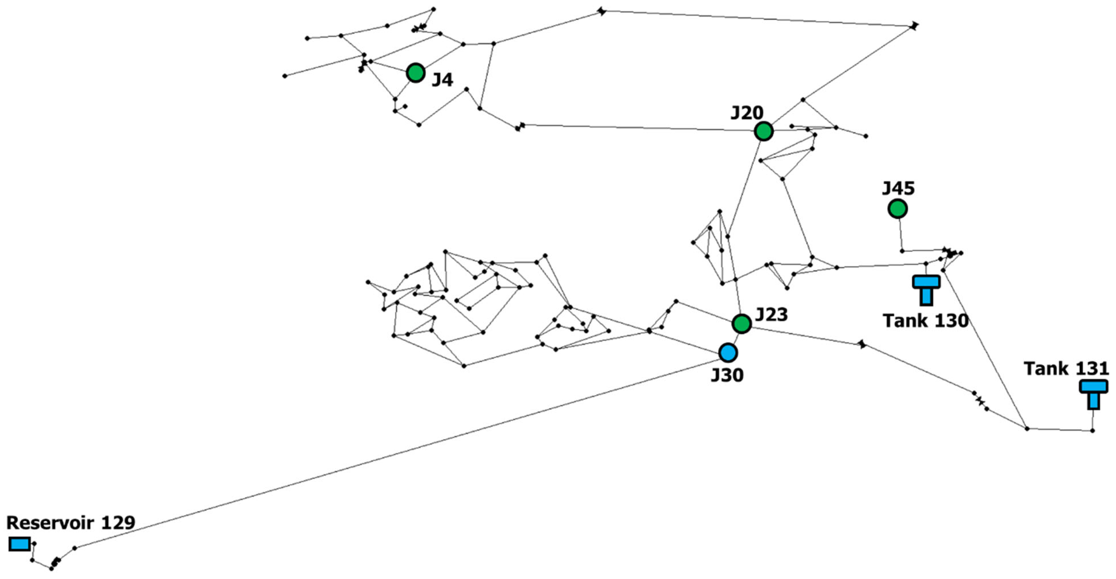
The North Marin Water District WDS or EPANET Example Network 3 (Supplementary Materials Figure S1), commonly used for WDS water quality modeling research, was selected as Test network 1 to demonstrate the applicability of EPANET-C. Test network 1 consists of 92 junctions, 2 pumps, 3 tanks, 2 source nodes (North Marin aqueduct (River) and Stafford Lake), and 117 pipes. The BWSN Network 1 [36], a real-life WDS that was renamed in order to preserve its anonymity (Figure 2) and is broadly used for water quality investigations, was selected as Test network 2. It has 4 variable demand patterns, and it is comprised of 126 junctions, 1 reservoir, 2 tanks, 2 pumps, 8 valves, and 168 pipes.
The water delivered from the source nodes of Test networks 1 and 2 were assumed to be treated by processes that are representative of characteristic physicochemical water treatment involving alum coagulation, dynamic settling, dual media filtration (sand and anthracite), and disinfection [61]. For our analysis, chlorine was selected as the disinfectant chemical. The TOC concentration and BDOC/TOC ratio of the treated water were taken from the value ranges reported in [62,63], respectively. The chosen THM concentration before delivery was 20 µg/L under chlorinated conditions and 0 µg/L under non-chlorinated conditions. The 2,4,6-TCP was assumed to exist in the water after treatment, and its concentration was adopted from [64]. For analysis, 2,4,6-TCA was presumed to be absent in the treated water before delivery. The water sources of Test networks 1 and 2 were assumed to be aqueous, film-forming, and foam-contaminated [65,66]. Thus, PFOAB and PFOAAmS were considered to be prevalent in the treated water. The fairly negligible effects of water treatment upon PFOAB and PFOAAmS elimination in the treatment plants were conveniently ignored. The PFOAB and PFOAAmS concentrations in the treated river and lake water sources prior to delivery were taken from the value ranges provided in the literature [67,68]. The PFOA concentration in the treated chlorinated water before delivery was assumed to be 3 ng/L [24]. For analysis, the temperature of the delivered water and the pH were fixed at 25 °C and 7.2, respectively, to meet the USEPA drinking water guidelines [69]. The characteristics of the source water quality in Test networks 1 and 2 considered for the analysis are detailed in Table 3.
Three (Cases 11, 12, and 13) and four (Cases 21, 22, 23, and 24) operating conditions were considered for Test network 1 and Test network 2, respectively. Cases 11, 12, and 13, corresponding to Test network 1, represent diverse chlorine and TOC loadings at the two water sources—River and Lake. Cases 11 and 12 correspond to chlorine concentrations of 1 and 0.5 mg/L of the treated water delivered from the river source. On the contrary, with water from the lake source, Case 13 corresponds to a TOC loading of 1.78 mg/L (a 50% reduction from the original TOC loading). The EPANET-C modules 1, 2, 3, 4, 12, 14, 24, 124, and 1234 were applied in Case 11, while only EPANET-C module 1234 was applied in Cases 12 and 13.
Case 21, corresponding to Test network 2, corresponds to no chlorine loading at the water source (Reservoir 129) and the intermediate nodes. On the contrary, Cases 22, 23, and 24 correspond to an induced booster chlorine dose (maintaining a chlorine concentration of 1 mg/L for the outflowing water parcels) at three separate intermediate locations—J30, Tank 130, and Tank 131. The EPANET-C module 1234 was applied to Cases 21–24 to simulate the microbial regrowth, THMs formation, T&O problem occurrence, and PFAS formation in Test network 2.
7. Results and Discussion
7.1. Test Network 1
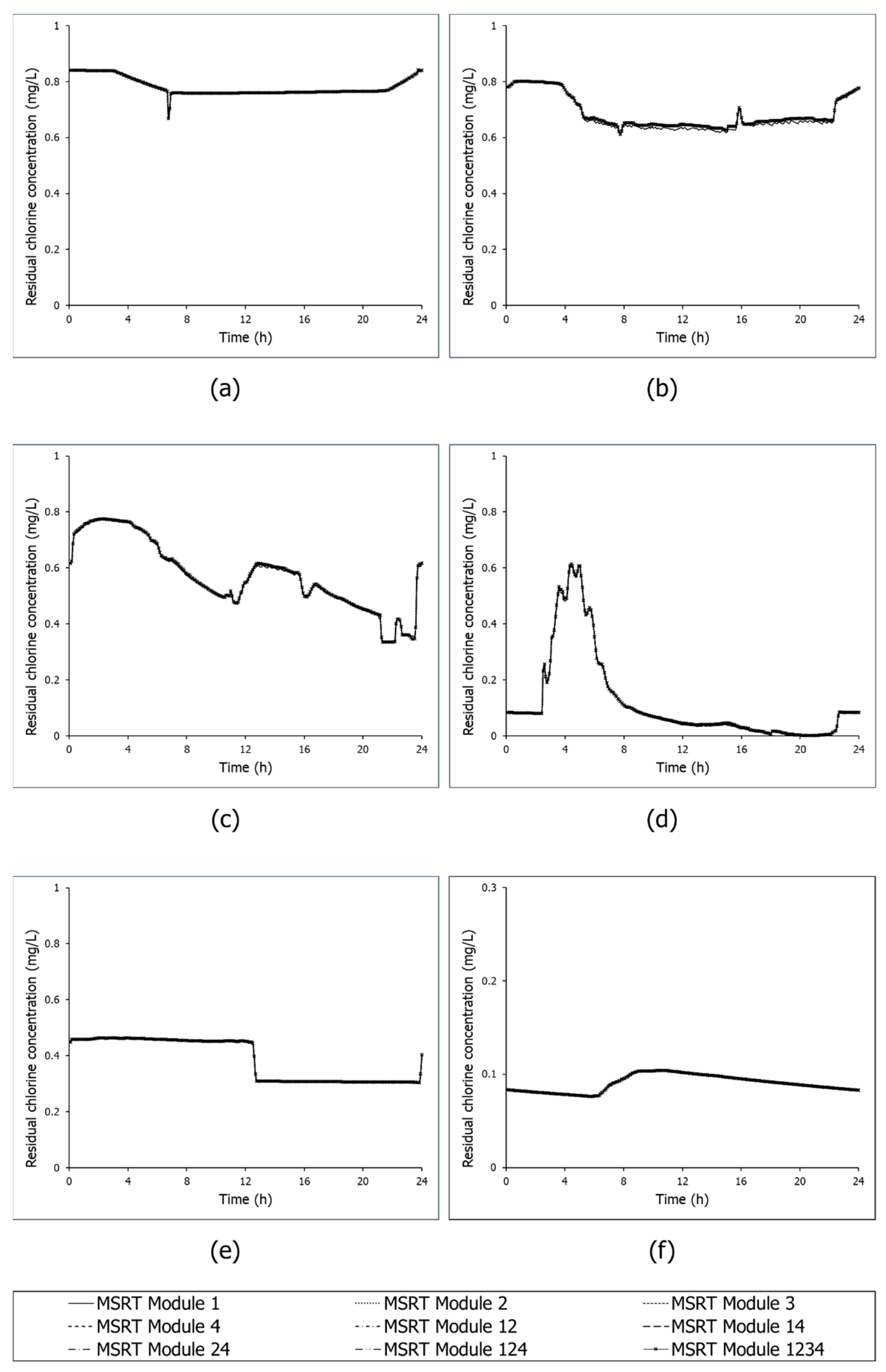
The 24 h variations in the residual chlorine concentrations at the six demand nodes of Test network 1 simulated with the use of nine MSRT modules of EPANET-C in Case 11 is depicted in Figure 3. The six network nodes (six junctions: J123, J161, J147, J255, and J131, and a tank: Tank 2) (Supplementary Materials Figure S1) with average water age values of 3.34, 10.18, 20.60, 40.09, 85.30, and 145.49 h were selected to cover the spatial extent of Test network 1. As can be observed in Figure 3, the residual chlorine concentration profiles predicted with the nine modules were found to be virtually similar. The maximum deviations amongst the different predictions were at <0.01%. This was expected since the chlorine–TOC reactions, the principal reactions corresponding to chlorine attenuation, remain the same in the governing equations of all the nine modules considered. While the other interactions related to chlorine decay (chlorine-PFOAB and chlorine-PFOAAmS reactions) and considered in the EPANET-C modules were practically significant, they were found to be irrelevant to the control of the chlorine dynamics in WDS.
Similar to chlorine, the TOC profiles obtained with the nine EPANET-C modules were also virtually indistinguishable (Supplementary Materials Figure S2). Furthermore, no disparities were distinguishable for THMs and PFOA concentration profiles (Supplementary Materials Figures S3 and S4). This could be attributed to the EPANET-C assumption that the THMs and PFOA formation are the by-products of the chlorine–TOC and chlorine–FA reactions. Hence, the kinetics of these reactions depends exclusively on the chlorine concentration values, which are predicted by the nine modules indistinctively.
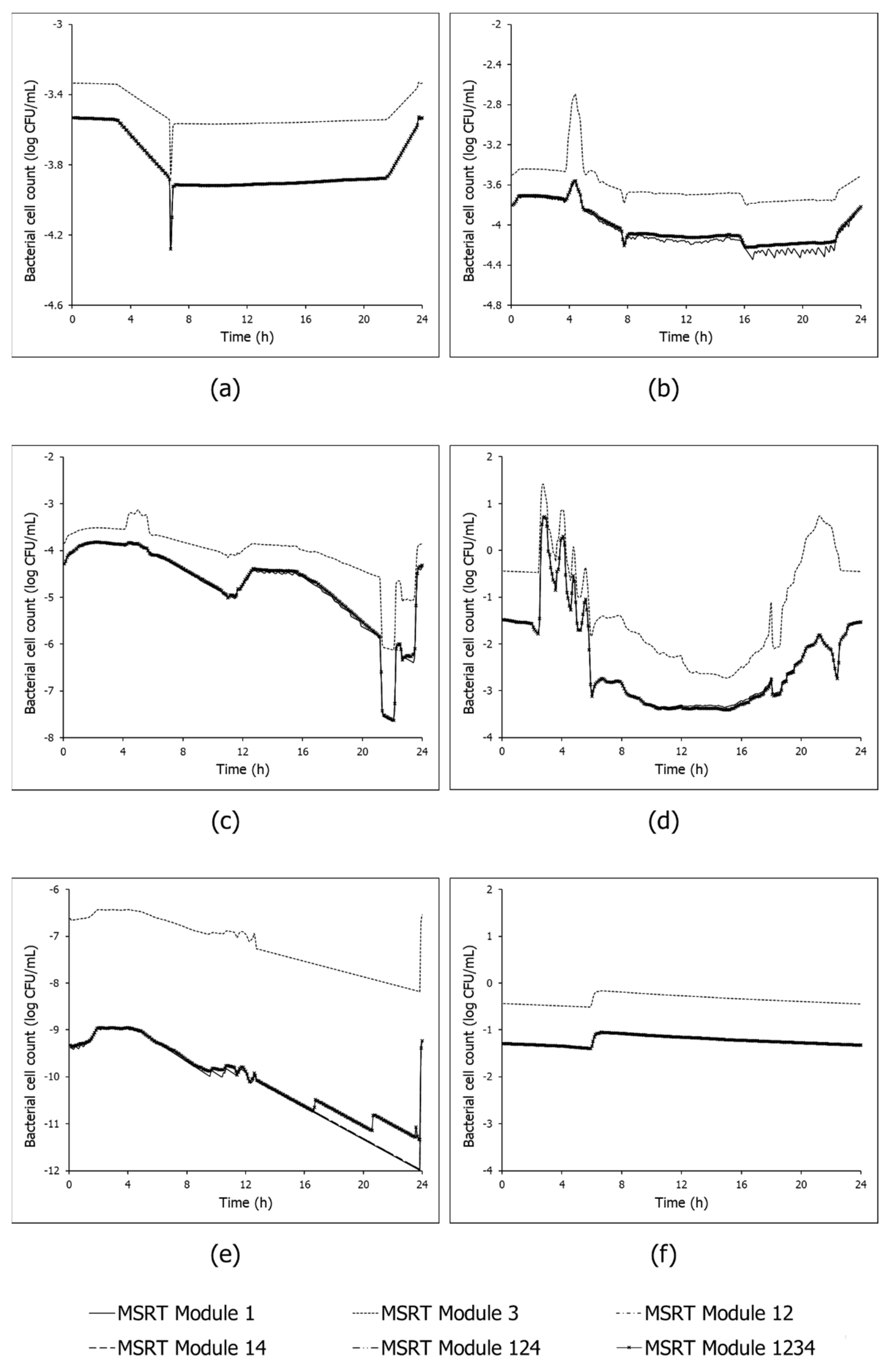
In contrast to the four parameters mentioned before, changes were primarily evident for the planktonic bacteria cell count and the 2,4,6-TCA concentration (Figure 4 and Supplementary Materials Figure S5). This could mainly be attributed to not incorporating the biofilm regrowth dynamics in the EPANET-C module 3, to focusing on the organoleptic quality variations, and to simplifying the microbial dynamics in its respective conceptual-mathematical framework. Thus, the processes such as the attachment of the planktonic bacterial cells to the biofilm layers and the detachment of attached bacterial cells from the biofilm layers were not incorporated in the EPANET-C module 3. The contradictions in the planktonic bacterial cell count estimates by the nine EPANET-C modules also impacted the predictions of 2,4,6-TCA formation. Clearly, the EPANET-C module 3 overpredicted the planktonic bacterial cell count and 2,4,6-TCA concentration values as compared to the other eight modules considered (Supplementary Materials Figure S5). These results shed light on the advantages and disadvantages of the diverse ways that the microbiological and organoleptic quality variations in WDS could possibly be evaluated. Altogether, the results also highlight the flexibility and competence of EPANET-C to simulate the behavior of the numerous contaminants in WDS and to examine the changes in quality of the delivered water.
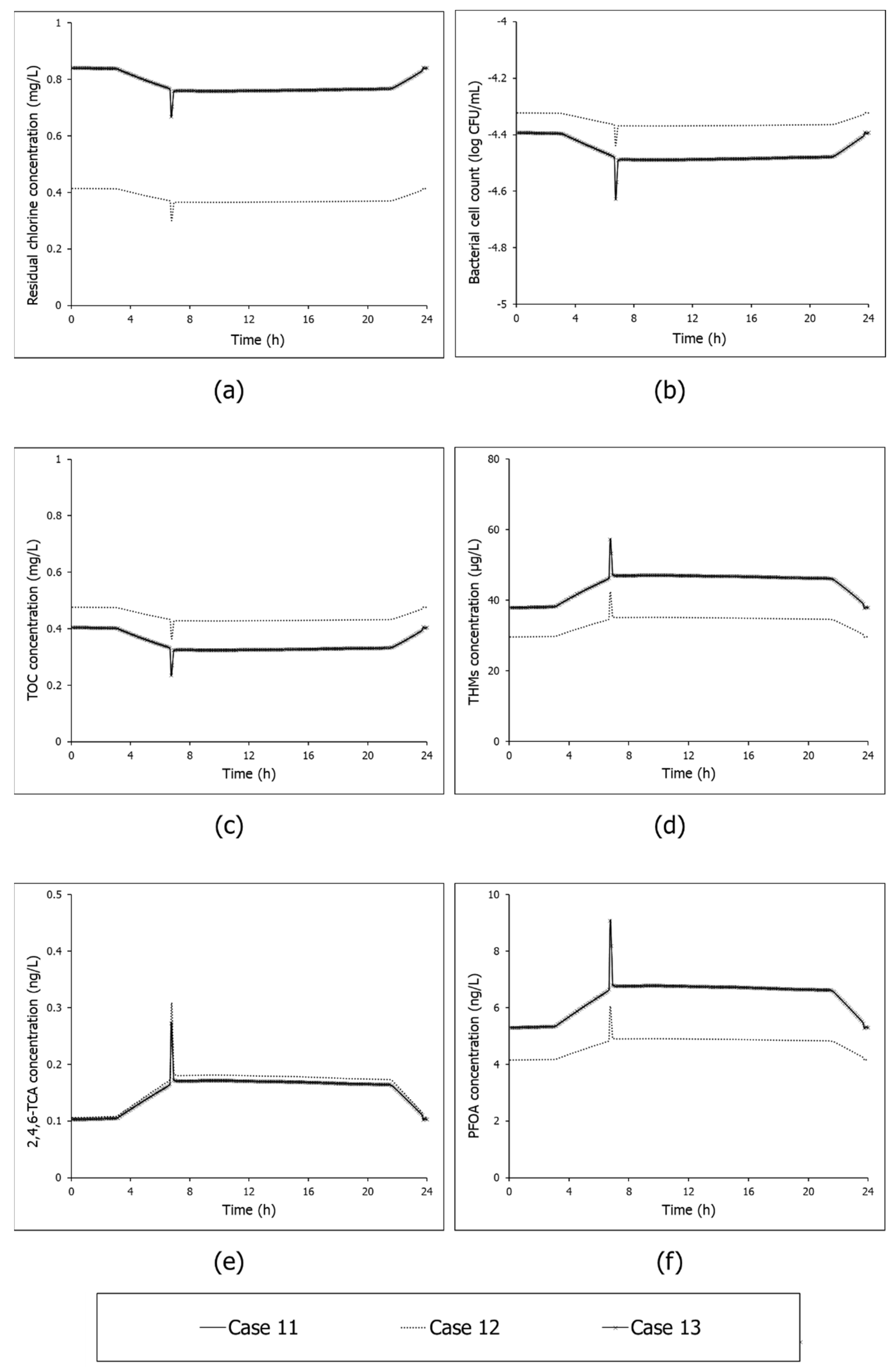
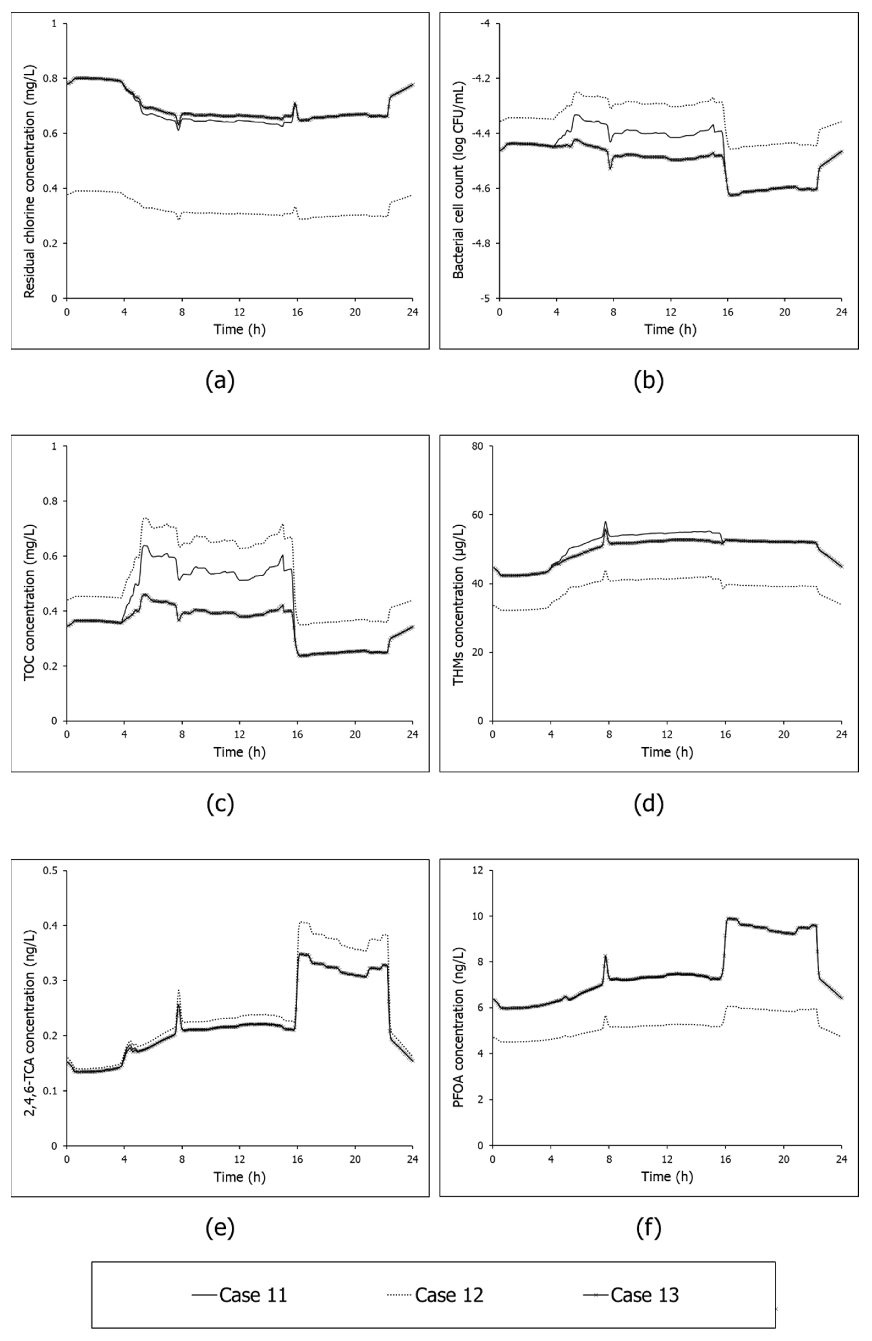
The 24 h variations in residual chlorine concentration, planktonic bacterial cell count, TOC concentration, THMs concentration, 2,4,6-TCA concentration, and PFOA concentration at the six network locations mentioned earlier, which were predicted with the module 1234 of EPANET-C for the three cases (Case 11–13), are shown in Figure 5 and Figure 6 and Supplementary Materials Figures S6–S9.
The results prove the competence of EPANET-C to produce time-series data that can be used as a standard for assessing the efficacy of WDS performance under different operating conditions, as considered in the case study here. Altogether, the results indicated that the operating condition corresponding to a 50% decrease in the chlorine dosing at the river source (identified as Case 12) was effective in decreasing the chemical contamination risks by reducing THM and PFOA formation in the delivered water. However, the simulation outputs also demonstrated the disadvantageous effects of decreased chlorine dosing (Case 12) on enhanced microbiological and organoleptic quality deterioration via increased bacterial regrowth and 2,4,6-TCA formation in the different nodes of Test network 1.
Fascinatingly, the modifications suggested in Case 13, which corresponds to TOC load reduction at the lake source, were found to have no impacts on the delivered water quality at two (out of six) network locations, i.e., J123 and J131. This can be attributed to the zero contribution of the lake source in the water demands at J123 and J131. Nonetheless, in the other four network locations considered (J161, J147, J255, and Tank 2), modified operating practice suggested that Case 13 was found to be superior to Cases 11 and 12 in reducing the microbiological and organoleptic quality deterioration. Intriguingly, Case 13 was found to be a better practice for reducing the THMs formation than Case 11, while the same was found to be inferior to Case 12 in administering the chlorine–TOC reactions. On the contrary, Case 13 was inferior to Cases 11 and 12 in governing the chlorine–FA reactions and the subsequent PFAS contamination of the delivered water.
7.2. Test Network 2
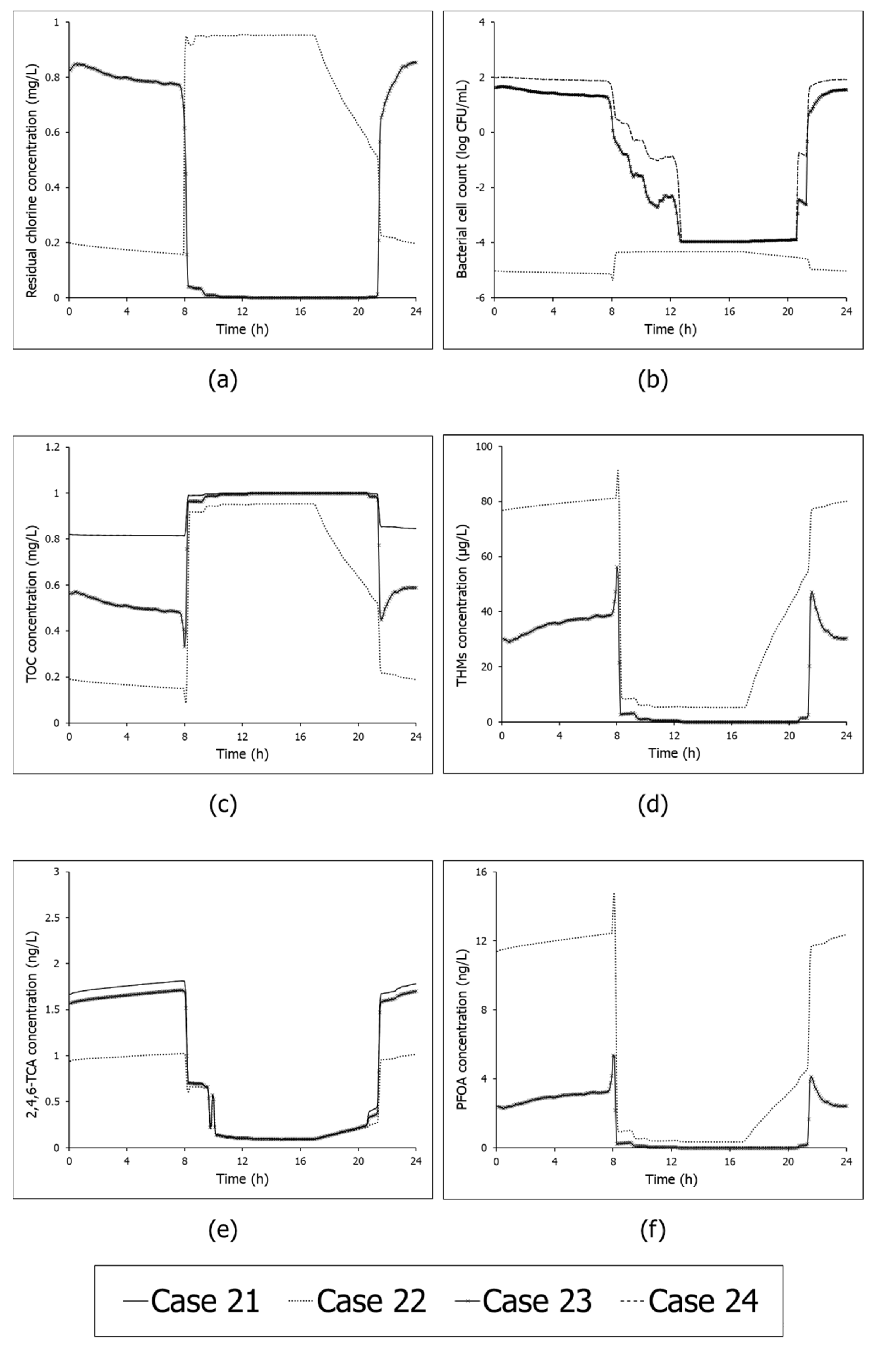
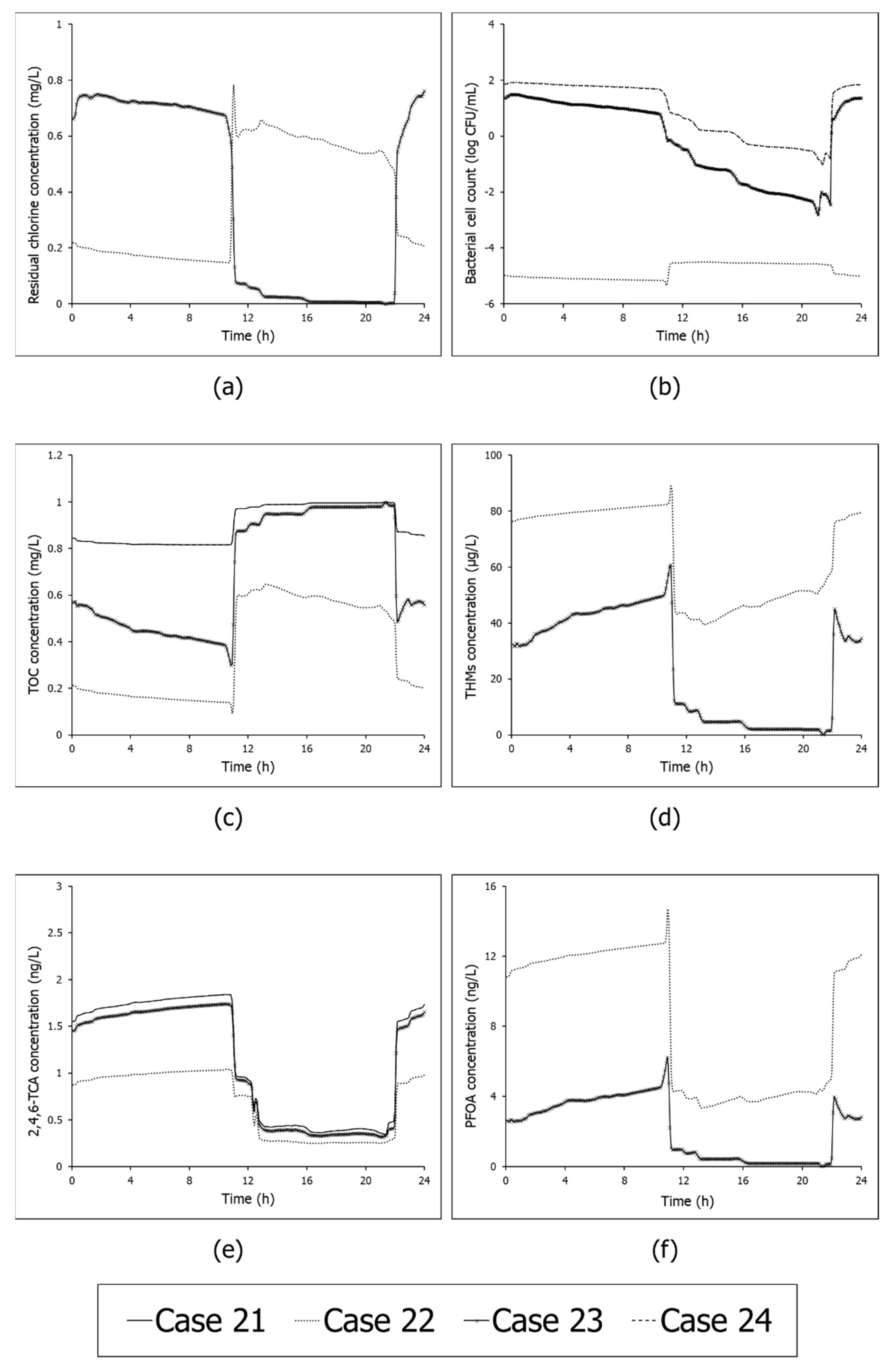
The 24 h profiles of the residual chlorine concentration, planktonic bacterial cell count, TOC concentration, THMs concentration, 2,4,6-TCA concentration, and PFOA concentration, which were predicted at four network locations (J23, J20, J45, and J4) of Test network 2 with the EPANET-C module 1234 for Cases 21–24, are shown in Figure 7 and Figure 8 and Supplementary Materials Figures S10 and S11. In Case 21, the bacterial cell count ranges obtained at the four nodes—J23, J20, J45, and J4—were 10.4–99.3 CFU/mL, 0.1–82.9 CFU/mL, 0.8–12.6 CFU/mL, and 0.2–46.7 CFU/mL, respectively. By inducing a booster chlorination at J30, the average log reductions in bacterial activity at the four benchmark locations were 4.1, 5.7, 5.2, and 6.0, respectively. However, in Case 23, the average log reductions in the bacterial activity effectuated by inducing the booster chlorination in Tank 130 at the four benchmark locations were 0.5, 1.1, 1.5, and 1.4, respectively. Intriguingly, booster chlorination in Tank 131 (Case 24) failed to introduce any impacts on the bacterial activity at J23, J20, J45, and J4 (Figure 7 and Figure 8 and Supplementary Materials Figures S10 and S11). As expected, the reduction in the microbiological activity in Cases 22 and 23 was reflected in the improvement of the organoleptic quality of the delivered water. The average percentage of reductions in the 2,4,6-TCA formation at the four locations mentioned earlier in Case 22 were 22.5, 38.5, 58.9, and 42.9%, respectively. Similar reductions in Case 23 were only 3.1, 7.6, 10.6, and 7.5, respectively.
Interestingly, an entirely different picture was obtained in terms of THM and PFOA formation in Cases 22 and 23. Although the practice of booster chlorination at both the nodes J30 (Case 22) and Tank 130 (Case 23) effectuated in increasing the DBP formation within the WDS, the average THM concentration at the four benchmark network locations in Case 22 was found to be about 17.4, 10.7, 27.2, and 5.4 times as that in Case 23. Likewise, the average PFOA concentration in the four benchmark network locations in Case 22 was about 14.6, 10.6, 36.7, and 6 times that in Case 23.
In sum, these results demonstrate the advantages of improving the microbiological and organoleptic quality, and the disadvantages of introducing chemical contamination risks by inducing booster chlorination at node J30 as compared to Tank 130 and 131. Furthermore, the results validate the applicability of EPANET-C in simulating intentional contamination events (booster chlorination) in WDS and in producing time-series data for the evaluation of WDS performance under non-chlorinated and chlorinated operating conditions.
8. Limitations of the Study and Future Scope
The proposed WDS contamination tool, EPANET-C, employs the computing environment of EPANET–EPANET-MSX. Therefore, it is afflicted with the numerical disadvantages of the default Lagrangian transport algorithm of EPANET and EPANET-MSX. Additionally, EPANET-C treats the contaminant transport within distribution pipes as a purely advective process, and thus, its suitability under dispersion-dominated flow conditions [70] needs to be re-ascertained. The MSRT modules of EPANET-C attempt to provide a broad picture of the bacterial interactions within WDS. Thus, to overcome the uncertainties related mainly to the heterogeneity of the microbial community within distribution pipes, EPANET-C chose a common bacterial strain (Pseudomonas) to simplify the interpretations of microbiological interactions in WDS. However, Pseudomonas cannot be recommended as the prototypical organism, and thus, EPANET-C overlooks the stochasticity corresponding to the microbial interactions within the WDS domain. The kinetic models defining the bioconversion of 2,4,6-TCP were adopted from the literature [33] to explain 2,4,6-TCA formation in WDS. However, due to the paucity of data, the effects of enzymatic synthesis, methyl donor distribution in the water, pipe material, water chemistry, and temperature on the microbial O-methylation mechanism effectuating the formation of 2,4,6-TCA were neglected. Hence, the kinetic model expressions require re-examination. The conceptual models of EPANET-C MSRT modules portray the multi-species reactions at a macroscopic scale and neglect the formation of intermediates and by-products. For this reason, the impacts of water chemistry on multi-species reactions and the ensuing implications go unaccounted for. Altogether, EPANET-C has limitations in explicitly portraying the stochasticity corresponding to WDS water quality variations. Therefore, future work should be aimed at addressing this problem.
9. Conclusions
This paper presented the development of a computer-based ‘umbrella’ WDS contamination simulation tool, EPANET-C, to aid the water supply managers in examining WDS performance under different operating scenarios. EPANET-C functions as an advanced extension of the EPANET–EPANET-MSX modeling. It uses function directories to integrate all the vital information relating to MSRT modeling in order to carry out WDS water quality analysis. In this way, EPANET-C bypasses the complications involved in the conceptual and mathematical modeling stages of MSRT modeling. EPANET-C also simplifies the execution of EPANET–EPANET-MSX by providing a simple command-line MATLAB interface equipped with an exhaustive set of instructions. In this way the users, even those lacking programming expertise, are enabled to execute WDS hydraulic and water quality modeling.
The applicability of EPANET-C was demonstrated by simulating the water quality variations in two well-tested benchmark WDS under different operating scenarios. The simulation outcomes established the potential of EPANET-C to generate time-series information regarding the WDS water quality parameter disparities, which can be used as yardsticks to evaluate WDS management strategies. Forthcoming works will expand on the EPANET-C capability in order to integrate the uncertainty in the knowledge about the mechanisms concerning water quality in WDS. Above and beyond, further reacting constituents and multi-species exchanges will be added to alter the conceptual-mathematical framework in order to improve the EPANET-C capability of simulating the formation, transmission, and health risks of several other conventional and non-conventional WDS contaminants.
Supplementary Materials
The following supporting information can be downloaded at: https://0-www-mdpi-com.brum.beds.ac.uk/article/10.3390/w14101665/s1, [71,72,73,74].
Author Contributions
Conceptualization, G.R.A.; methodology, G.R.A. and A.O.; writing—original draft preparation, G.R.A.; writing—review and editing, A.O.; supervision, A.O.; project administration, A.O.; funding acquisition, A.O. All authors have read and agreed to the published version of the manuscript.
Funding
This research was supported by a grant from the Ministry of Science and Technology of the State of Israel and the Federal Ministry of Education and Research (BMBF), Germany.
Institutional Review Board Statement
Not Applicable.
Informed Consent Statement
Not Applicable.
Data Availability Statement
The data presented in this study are available on request from the corresponding author.
Conflicts of Interest
The authors declare no conflict of interest.
References
- Liang, J.L.; Dziuban, E.J.; Craun, G.F.; Hill, V.; Moore, M.R.; Gelting, R.J.; Calderon, R.L.; Beach, M.J.; Roy, S.L. Surveillance for waterborne disease and outbreaks associated with drinking water and water not intended for drinking—United States, 2003–2004. Morb. Mortal. Wkly. Rep. Surveill. Summ. 2006, 55, 31–65. [Google Scholar]
- Gavriel, A.A.; Landre, J.P.B.; Lamb, A.J. Incidence of mesophilic Aeromonas within a public drinking water supply in north-east Scotland. J. Appl. Microbiol. 1998, 84, 383–392. [Google Scholar] [CrossRef] [PubMed]
- Yokoyama, K. Our recent experiences with sarin poisoning cases in Japan and pesticide users with references to some selected chemicals. Neurotoxicology 2007, 28, 364–373. [Google Scholar] [CrossRef] [PubMed]
- Lifshitz, R.; Ostfeld, A. Clustering for Real-Time Response to Water Distribution System Contamination Event Intrusions. J. Water Resour. Plan. Manag. 2019, 145, 04018091. [Google Scholar] [CrossRef]
- Clark, R.M. The USEPA’s distribution system water quality modelling program: A historical perspective. Water Environ. J. 2015, 29, 320–330. [Google Scholar] [CrossRef]
- Liou, C.P.; Kroon, J.R. Modeling the Propagation of Waterborne Substances in Distribution Networks. J. Am. Water Work. Assoc. 1987, 79, 54–58. [Google Scholar] [CrossRef]
- Grayman, W.M.; Clark, R.M.; Males, R.M. Modeling Distribution-System Water Quality: Dynamic Approach. J. Water Resour. Plan. Manag. 1988, 114, 295–312. [Google Scholar] [CrossRef]
- Abhijith, G.R.; Mohan, S. Random Walk Particle Tracking embedded Cellular Automata model for predicting temporospatial variations of chlorine in water distribution systems. Environ. Process. 2020, 7, 271–296. [Google Scholar] [CrossRef]
- Rossman, L.A.; Boulos, P.F.; Altman, T. Discrete Volume-Element Method for Network Water-Quality Models. J. Water Resour. Plan. Manag. 1993, 119, 505–517. [Google Scholar] [CrossRef] [Green Version]
- Boulos, P.F.; Altman, T.; Jarrige, P.A.; Collevati, F. An event-driven method for modelling contaminant propagation in water networks. Appl. Math. Model. 1994, 18, 84–92. [Google Scholar] [CrossRef]
- Axworthy, D.H.; Karney, B.W. Modeling Low Velocity/High Dispersion Flow in Water Distribution systems. J. Water Resour. Plan. Manag. 1996, 122, 218–221. [Google Scholar] [CrossRef]
- Helbling, D.E.; VanBriesen, J.M. Modeling Residual Chlorine Response to a Microbial Contamination Event in Drinking Water Distribution Systems. J. Environ. Eng. 2009, 135, 918–927. [Google Scholar] [CrossRef]
- Aisopou, A.; Stoianov, I.; Graham, N.J.D. Modelling Chlorine Transport under Unsteady-State Hydraulic Conditions. Water Distrib. Syst. Anal. 2010, 2010, 613–625. [Google Scholar] [CrossRef]
- Monteiro, L.; Figueiredo, D.; Dias, S.; Freitas, R.; Covas, D.; Menaia, J.; Coelho, S.T. Modeling of chlorine decay in drinking water supply systems using EPANET MSX. Procedia Eng. 2014, 70, 1192–1200. [Google Scholar] [CrossRef] [Green Version]
- Monteiro, L.; Carneiro, J.; Covas, D.I.C. Modelling chlorine wall decay in a full-scale water supply system. Urban Water J. 2020, 17, 754–762. [Google Scholar] [CrossRef]
- Kim, H.; Kim, S.; Koo, J. Modelling chlorine decay in a pilot scale water distribution system subjected to transient. Procedia Eng. 2015, 119, 370–378. [Google Scholar] [CrossRef]
- Lu, C.; Biswas, P.; Clark, R.M. Simultaneous transport of substrates, disinfectants and microorganisms in water pipes. Water Res. 1995, 29, 881–894. [Google Scholar] [CrossRef]
- Servais, P.; Laurent, P.; Billen, G.; Gatel, D. Development of a Model of BDOC and Bacterial Biomass Fluctuations in Distribution Systems. Rev. Sci. Eau 1995, 8, 427–462. [Google Scholar]
- Ohar, Z.; Ostfeld, A.; Lahav, O.; Birnhack, L. Modelling heavy metal contamination events in water distribution systems. Procedia Eng. 2015, 119, 328–336. [Google Scholar] [CrossRef] [Green Version]
- Klosterman, S.; Murray, R.; Szabo, J.; Hall, J.; Uber, J. Modeling and simultation of arsenate fate and transport in a distribution system simulator. In Water Distribution Systems Analysis 2010, Proceedings of the 12th Annual Conference on Water Distribution Systems Analysis (WDSA), Tucson, AZ, USA, 12–15 September 2010; American Society of Civil Engineers: Reston, VA, USA, 2012; pp. 655–669. [Google Scholar] [CrossRef] [Green Version]
- Burkhardt, J.B.; Szabo, J.; Klosterman, S.; Hall, J.; Murray, R. Modeling fate and transport of arsenic in a chlorinated distribution system. Environ. Model. Softw. 2017, 93, 322–331. [Google Scholar] [CrossRef] [Green Version]
- Abokifa, A.A.; Biswas, P. Modeling Soluble and Particulate Lead Release into Drinking Water from Full and Partially Replaced Lead Service Lines. Environ. Sci. Technol. 2017, 51, 3318–3326. [Google Scholar] [CrossRef] [PubMed]
- Munavalli, G.R.; MohanKumar, M.S. Dynamic simulation of multicomponent reaction transport in water distribution systems. Water Res. 2004, 38, 1971–1988. [Google Scholar] [CrossRef] [PubMed]
- Abhijith, G.R.; Ostfeld, A. Model-based investigation of the formation, transmission, and health risk of perfluorooctanoic acid, a member of PFASs group, in drinking water distribution systems. Water Res. 2021, 204, 117626. [Google Scholar] [CrossRef] [PubMed]
- Abhijith, G.R.; Ostfeld, A. Modeling the Response of Nonchlorinated, Chlorinated, and Chloraminated Water Distribution Systems toward Arsenic Contamination. J. Environ. Eng. 2021, 147, 04021045. [Google Scholar] [CrossRef]
- Dukan, S.; Levi, Y.; Piriou, P.; Guyon, F.; Villon, P. Dynamic modelling of bacterial growth in drinking water networks. Water Res. 1996, 30, 1991–2002. [Google Scholar] [CrossRef]
- Bois, F.Y.; Fahmy, T.; Block, J.C.; Gatel, D. Dynamic modeling of bacteria in a pilot drinking-water distribution system. Water Res. 1997, 31, 3146–3156. [Google Scholar] [CrossRef]
- Zhang, W.; Miller, C.T.; DiGiano, F.A. Bacterial Regrowth Model for Water Distribution Systems Incorporating Alternating Split-Operator Solution Technique. J. Environ. Eng. 2004, 130, 932–941. [Google Scholar] [CrossRef]
- Abokifa, A.A.; Yang, Y.J.; Lo, C.S.; Biswas, P. Investigating the role of biofilms in trihalomethane formation in water distribution systems with a multicomponent model. Water Res. 2016, 104, 208–219. [Google Scholar] [CrossRef]
- Chen, G.; Long, T.; Bai, Y. Water quality model with axial dispersion solved by Eulerian-Lagrangian operator-splitting method in water distribution system. Water Sci. Technol. Water Supply 2017, 18, 831–842. [Google Scholar] [CrossRef]
- Abhijith, G.R.; Mohan, S. Cellular Automata-based Mechanistic Model for Analyzing Microbial Regrowth and Trihalomethanes Formation in Water Distribution Systems. J. Environ. Eng. 2021, 147, 04020145. [Google Scholar] [CrossRef]
- Abhijith, G.R.; Kadinski, L.; Ostfeld, A. Modeling Bacterial Regrowth and Trihalomethane Formation in Water Distribution Systems. Water 2021, 13, 463. [Google Scholar] [CrossRef]
- Abhijith, G.R.; Ostfeld, A. Modeling the Formation and Propagation of 2,4,6-trichloroanisole, a Dominant Taste and Odor Compound, in Water Distribution Systems. Water 2021, 13, 638. [Google Scholar] [CrossRef]
- Rossman, L.A. EPANET 2: Users Manual; United States Environmental Protection Agency: Washington, DC, USA, 2000.
- Shang, F.; Uber, J.G.; Rossman, L.A. EPANET Multi-Species Extension User’s Manual; United States Environmental Protection Agency: Washington, DC, USA, 2007; p. 115.
- Ostfeld, A.; Uber, J.G.; Salomons, E.; Berry, J.W.; Hart, W.E.; Phillips, C.A.; Watson, J.-P.; Dorini, G.; Jonkergouw, P.; Kapelan, Z.; et al. The Battle of the Water Sensor Networks (BWSN): A Design Challenge for Engineers and Algorithms. J. Water Resour. Plan. Manag. 2008, 134, 556–568. [Google Scholar] [CrossRef] [Green Version]
- Huck, P.M. Measurement of biodegradable organic matter and bacterial growth potential in drinking water. J. Am. Water Work. Assoc. 1990, 82, 78–86. [Google Scholar] [CrossRef]
- Clark, R.M.; Sivaganesan, M. Predicting Chlorine Residuals in Drinking Water: Second Order Model. J. Water Resour. Plan. Manag. 2002, 128, 152–161. [Google Scholar] [CrossRef]
- Sohn, J.; Amy, G.; Cho, J.; Lee, Y.; Yoon, Y. Disinfectant decay and disinfection by-products formation model development: Chlorination and ozonation by-products. Water Res. 2004, 38, 2461–2478. [Google Scholar] [CrossRef]
- Tsitsifli, S.; Kanakoudis, V. Determining hazards’ prevention critical control points in water supply systems. Environ. Sci. Proc. 2020, 2, 53. [Google Scholar] [CrossRef]
- Peter, A.; Von Gunten, U. Taste and odour problems generated in distribution systems: A case study on the formation of 2,4,6-trichloroanisole. J. Water Supply Res. Technol. AQUA 2009, 58, 386–394. [Google Scholar] [CrossRef]
- Chen, X.; Luo, Q.; Yuan, S.; Wei, Z.; Song, H.; Wang, D.; Wang, Z. Simultaneous determination of ten taste and odor compounds in drinking water by solid-phase microextraction combined with gas chromatography-mass spectrometry. J. Environ. Sci. 2013, 25, 2313–2323. [Google Scholar] [CrossRef]
- Nystrom, A.; Grimvall, A.; Krantz-Rulcker, C.; Savenhed, R.; Akerstrand, K. Drinking water off-flavour caused by 2,4,6-trichloroanisole. Water Sci. Technol. 1992, 25, 241–249. [Google Scholar] [CrossRef]
- Zhang, N.; Xu, B.; Qi, F.; Kumirska, J. The occurrence of haloanisoles as an emerging odorant in municipal tap water of typical cities in China. Water Res. 2016, 98, 242–249. [Google Scholar] [CrossRef] [PubMed]
- Malleret, L.; Bruchet, A.; Hennion, M.C. Picogram determination of “earthy-musty” odorous compounds in water using modified closed loop stripping analysis and large volume injection GC/MS. Anal. Chem. 2001, 73, 1485–1490. [Google Scholar] [CrossRef]
- Richardson, S.D.; DeMarini, D.M.; Kogevinas, M.; Fernandez, P.; Marco, E.; Lourencetti, C.; Ballesté, C.; Heederik, D.; Meliefste, K.; McKague, A.B.; et al. What’s in the pool? a comprehensive identification of disinfection by-products and assessment of mutagenicity of chlorinated and brominated swimming pool water. Environ. Health Perspect. 2010, 118, 1523–1530. [Google Scholar] [CrossRef] [PubMed] [Green Version]
- Lennard, L. Methyltransferases. In Comprehensive Toxicology, 2nd ed.; McQueen, C.A., Ed.; Elsevier: Oxford, UK, 2010; pp. 435–457. ISBN 978-0-08-046884-6. [Google Scholar]
- Zhang, K.; Luo, Z.; Zhang, T.; Mao, M.; Fu, J. Study on formation of 2,4,6-trichloroanisole by microbial O-methylation of 2,4,6-trichlorophenol in lake water. Environ. Pollut. 2016, 219, 228–234. [Google Scholar] [CrossRef] [PubMed]
- Buck, R.C.; Franklin, J.; Berger, U.; Conder, J.M.; Cousins, I.T.; De Voogt, P.; Jensen, A.A.; Kannan, K.; Mabury, S.A.; van Leeuwen, S.P.J. Perfluoroalkyl and polyfluoroalkyl substances in the environment: Terminology, classification, and origins. Integr. Environ. Assess. Manag. 2011, 7, 513–541. [Google Scholar] [CrossRef]
- USEPA. Drinking Water Health Advisory for Perfluorooctanoic Acid (PFOA); USEPA: Washington, DC, USA, 2016.
- Xiao, F.; Hanson, R.A.; Golovko, S.A.; Golovko, M.Y.; Arnold, W.A. PFOA and PFOS Are Generated from Zwitterionic and Cationic Precursor Compounds during Water Disinfection with Chlorine or Ozone. Environ. Sci. Technol. Lett. 2018, 5, 382–388. [Google Scholar] [CrossRef]
- Rożej, A.; Cydzik-Kwiatkowska, A.; Kowalska, B.; Kowalski, D. Structure and microbial diversity of biofilms on different pipe materials of a model drinking water distribution systems. World J. Microbiol. Biotechnol. 2015, 31, 37–47. [Google Scholar] [CrossRef] [Green Version]
- Bertelli, C.; Courtois, S.; Rosikiewicz, M.; Piriou, P.; Aeby, S.; Robert, S.; Loret, J.F.; Greub, G. Reduced chlorine in drinking water distribution systems impacts bacterial biodiversity in biofilms. Front. Microbiol. 2018, 9, 1–11. [Google Scholar] [CrossRef] [Green Version]
- Joannis, C.; Delia, M.L.; Riba, J.P. Comparison of four methods for quantification of biofilms in biphasic cultures. Biotechnol. Tech. 1998, 12, 777–782. [Google Scholar] [CrossRef] [Green Version]
- Péquignot, C.; Larroche, C.; Gros, J.B. A spectrophotometric method for determination of bacterial biomass in the presence of a polymer. Biotechnol. Tech. 1998, 12, 899–903. [Google Scholar] [CrossRef]
- Kim, D.; Chung, S.; Lee, S.; Choi, J. Relation of microbial biomass to counting units for Pseudomonas aeruginosa. Afr. J. Microbiol. Res. 2012, 6, 4620–4622. [Google Scholar] [CrossRef]
- Rossman, L.A.; Clark, R.M.; Grayman, W.M. Modeling Chlorine Residuals in Drinking-Water Distribution Systems. J. Environ. Eng. 1994, 120, 803–820. [Google Scholar] [CrossRef]
- Horn, H.; Reiff, H.; Morgenroth, E. Simulation of growth and detachment in biofilm systems under defined hydrodynamic conditions. Biotechnol. Bioeng. 2003, 81, 607–617. [Google Scholar] [CrossRef] [PubMed]
- Schrottenbaum, I.; Uber, J.; Ashbolt, N.; Murray, R.; Janke, R.; Szabo, J.; Boccelli, D. Simple Model of Attachment and Detachment of Pathogens in Water Distribution System Biofilms. In Proceedings of the World Environmental and Water Resources Congress 2009, Kansas City, MO, USA, 17–21 May 2009; ASCE: Reston, VA, USA, 2009; pp. 145–157. [Google Scholar]
- Eliades, D.G.; Kyriakou, M.; Vrachimis, S.G.; Polycarpou, M.M. EPANET-MATLAB Toolkit: An Open-Source Software for Interfacing EPANET with MATLAB. In Proceedings of the Computing and Control for the Water Industry CCWI 2016, Amsterdam, The Netherlands, 7–9 November 2016; pp. 1–8. [Google Scholar]
- Prévost, M.; Rompré, A.; Coallier, J.; Servais, P.; Laurent, P.; Clément, B.; Lafrance, P. Suspended bacterial biomass and activity in full-scale drinking water distribution systems: Impact of water treatment. Water Res. 1998, 32, 1393–1406. [Google Scholar] [CrossRef]
- Vasconcelos, J.J.; Rossman, L.A.; Grayman, W.M.; Boulos, P.F.; Clark, R.M. Kinetics of chlorine decay. J. Am. Water Work. Assoc. 1997, 89, 54–65. [Google Scholar] [CrossRef]
- Prest, E.I.; Hammes, F.; van Loosdrecht, M.C.M.; Vrouwenvelder, J.S. Biological stability of drinking water: Controlling factors, methods, and challenges. Front. Microbiol. 2016, 7, 1–24. [Google Scholar] [CrossRef]
- Zhang, K.; Cao, C.; Zhou, X.; Zheng, F.; Sun, Y.; Cai, Z.; Fu, J. Pilot investigation on formation of 2,4,6-trichloroanisole via microbial O-methylation of 2,4,6-trichlorophenol in drinking water distribution system: An insight into microbial mechanism. Water Res. 2018, 131, 11–21. [Google Scholar] [CrossRef]
- Backe, W.J.; Day, T.C.; Field, J.A. Zwitterionic, cationic, and anionic fluorinated chemicals in aqueous film forming foam formulations and groundwater from U.S. military bases by nonaqueous large-volume injection HPLC-MS/MS. Environ. Sci. Technol. 2013, 47, 5226–5234. [Google Scholar] [CrossRef]
- Barzen-Hanson, K.A.; Roberts, S.C.; Choyke, S.; Oetjen, K.; McAlees, A.; Riddell, N.; McCrindle, R.; Ferguson, P.L.; Higgins, C.P.; Field, J.A. Discovery of 40 Classes of Per- and Polyfluoroalkyl Substances in Historical Aqueous Film-Forming Foams (AFFFs) and AFFF-Impacted Groundwater. Environ. Sci. Technol. 2017, 51, 2047–2057. [Google Scholar] [CrossRef]
- Boiteux, V.; Dauchy, X.; Bach, C.; Colin, A.; Hemard, J.; Sagres, V.; Rosin, C.; Munoz, J.F. Concentrations and patterns of perfluoroalkyl and polyfluoroalkyl substances in a river and three drinking water treatment plants near and far from a major production source. Sci. Total Environ. 2017, 583, 393–400. [Google Scholar] [CrossRef]
- Evans, S.; Andrews, D.; Stoiber, T.; Naidenko, O. PFAS Contamination of Drinking Water Far More Prevalent than Previously Reported—New Detections of ‘Forever Chemicals’ in New York, D.C., Other Major Cities. Available online: https://www.ewg.org/research/national-pfas-testing/ (accessed on 26 March 2021).
- USEPA. National Primary Drinking Water Guidelines. Available online: https://www.epa.gov/sites/production/files/2016-06/documents/npwdr_complete_table.pdf (accessed on 22 February 2021).
- Abhijith, G.R.; Ostfeld, A. Examining the Longitudinal Dispersion of Solutes Inside Water Distribution Systems. J. Water Resour. Plan. Manag. 2022, 148, 04022022. [Google Scholar] [CrossRef]
- Kiene, L.; Lu, W.; Levi, Y. Relative importance of the phenomena responsible for chlorine decay in drinking water distribution systems. Water Sci. Technol. 1998, 38, 219–227. [Google Scholar]
- Camper, A.K. Factors Limiting Microbial Growth in Distribution Systems: Laboratory and Pilot-Scale Experiments; AWWA Research Foundation and AWWA: Denver, CO, USA, 1996; ISBN 1583210512. [Google Scholar]
- Billen, G.; Servais, P.; Ventresque, C. Functioning of biological filters used in drinking-water treatment—The Chabrol model. J. Water Supply Res. Technol. 1992, 41, 231–241. [Google Scholar]
- Clark, R.M. Chlorine demand and TTHM formation kinetics: A second-order model. J. Environ. Eng. 1998, 124, 16–24. [Google Scholar] [CrossRef]
Figure 1.
Conceptual framework of the EPANET-C MSRT Module 1234.

Figure 2.
Schematic of BWSN Network 1 (Test network 1).

Figure 3.
Twenty-four-hour variations in residual chlorine concentrations simulated with EPANET-C Modules 1, 2, 3, 4, 12, 14, 24, 124, and 1234 at network locations (a) J123, (b) J161, (c) J147, (d) J255, (e) J131, and (f) Tank 2 of Test network 1.
Figure 3.
Twenty-four-hour variations in residual chlorine concentrations simulated with EPANET-C Modules 1, 2, 3, 4, 12, 14, 24, 124, and 1234 at network locations (a) J123, (b) J161, (c) J147, (d) J255, (e) J131, and (f) Tank 2 of Test network 1.

Figure 4.
Twenty-four-hour variations in planktonic bacterial cell count simulated with EPANET-C Modules 1, 3, 12, 14, 124, and 1234 at network locations (a) J123, (b) J161, (c) J147, (d) J255, (e) J131, and (f) Tank 2 of Test network 1.
Figure 4.
Twenty-four-hour variations in planktonic bacterial cell count simulated with EPANET-C Modules 1, 3, 12, 14, 124, and 1234 at network locations (a) J123, (b) J161, (c) J147, (d) J255, (e) J131, and (f) Tank 2 of Test network 1.

Figure 5.
Twenty-four-hour variations in (a) residual chlorine concentration, (b) planktonic bacterial cell count, (c) TOC concentration, (d) THMs concentration, (e) 2,4,6-TCA concentration, and (f) PFOA concentration simulated with EPANET-C Module 1234 in Cases 11, 12, and 13 at network location J123 of Test network 1.

Figure 6.
Twenty-four-hour variations in (a) residual chlorine concentration, (b) planktonic bacterial cell count, (c) TOC concentration, (d) THMs concentration, (e) 2,4,6-TCA concentration, and (f) PFOA concentration simulated with EPANET-C Module 1234 in Cases 11, 12, and 13 at network location J161 of Test network 1.

Figure 7.
Twenty-four-hour variations in (a) residual chlorine concentration, (b) planktonic bacterial cell count, (c) TOC concentration, (d) THMs concentration, (e) 2,4,6-TCA concentration, and (f) PFOA concentration simulated with EPANET-C Module 1234 in Cases 21, 22, 23, and 24 at network location J23 of Test network 2.

Figure 8.
Twenty-four-hour variations in (a) residual chlorine concentration, (b) planktonic bacterial cell count, (c) TOC concentration, (d) THMs concentration, (e) 2,4,6-TCA concentration, and (f) PFOA concentration simulated with EPANET-C Module 1234 in Cases 21, 22, 23, and 24 at network location J20 of Test network 2.


Table 1.
Details of the MSRT modules of EPANET-C.
| S. No. | Notation | EPANET-C Module Title | Reacting Constituents |
|---|---|---|---|
| 1 | 1 | Microbial regrowth model | Chlorine, planktonic bacteria, biofilm bacteria, TOC, and BDOC |
| 2 | 2 | Trihalomethanes formation model | Chlorine, TOC, and THMs |
| 3 | 3 | 2,4,6-trichloroanisole formation model | Chlorine, planktonic bacteria, TOC, BDOC, 2,4,6-TCP, and 2,4,6-TCA |
| 4 | 4 | PFOA formation model | Chlorine, TOC, PFOAB, PFOAAmS, and PFOA |
| 5 | 12 | Microbial regrowth and trihalomethanes formation model | Chlorine, planktonic bacteria, biofilm bacteria, TOC, BDOC, and THMs |
| 6 | 13 | Microbial regrowth and 2,4,6-trichloroanisole formation model | Chlorine, planktonic bacteria, biofilm bacteria, TOC, BDOC, 2,4,6-TCP, and 2,4,6-TCA |
| 7 | 14 | Microbial regrowth and PFOA formation model | Chlorine, planktonic bacteria, biofilm bacteria, TOC, BDOC, PFOAB, PFOAAmS, and PFOA |
| 8 | 23 | Trihalomethanes and 2,4,6-trichloroanisole formation model | Chlorine, planktonic bacteria, TOC, BDOC, THMs, 2,4,6-TCP, and 2,4,6-TCA |
| 9 | 24 | Trihalomethanes and PFOA formation model | Chlorine, TOC, THMs, PFOAB, PFOAAmS, and PFOA |
| 10 | 34 | 2,4,6-trichloroanisole and PFOA formation model | Chlorine, planktonic bacteria, TOC, BDOC, 2,4,6-TCP, 2,4,6-TCA, PFOAB, PFOAAmS, and PFOA |
| 11 | 123 | Microbial regrowth, trihalomethanes formation, and 2,4,6-trichloroanisole formation model | Chlorine, planktonic bacteria, biofilm bacteria, TOC, BDOC, THMs, 2,4,6-TCP, and 2,4,6-TCA |
| 12 | 124 | Microbial regrowth, trihalomethanes formation, and PFOA formation model | Chlorine, planktonic bacteria, biofilm bacteria, TOC, BDOC, THMs, PFOAB, PFOAAmS, and PFOA |
| 13 | 134 | Microbial regrowth, 2,4,6-trichloroanisole formation, and PFOA formation model | Chlorine, planktonic bacteria, biofilm bacteria, TOC, BDOC, 2,4,6-TCP, 2,4,6-TCA, PFOAB, PFOAAmS, and PFOA |
| 14 | 234 | Trihalomethanes formation, 2,4,6-trichloroanisole formation, and PFOA formation model | Chlorine, planktonic bacteria, TOC, BDOC, THMs, 2,4,6-TCP, 2,4,6-TCA, PFOAB, PFOAAmS, and PFOA |
| 15 | 1234 | Microbial regrowth, trihalomethanes formation, 2,4,6-trichloroanisole formation, and PFOA formation model | Chlorine, planktonic bacteria, biofilm bacteria, TOC, BDOC, THMs, 2,4,6-TCP, 2,4,6-TCA, PFOAB, PFOAAmS, and PFOA |
Table 2.
Non-mandatory inputs, existing options, and default values of EPANET-C.
| S. No | Input | Options | Default Value |
|---|---|---|---|
| 1 | Area units | m2 cm2 ft2 | m2 ft2 |
| 2 | Rate units | s min h day | day |
| 3 | Numerical integration method | Standard Euler integrator Runge–Kutta 5th order integrator 2nd order Rosenbrock integrator | Standard Euler integrator |
| 4 | Simulation time step | - | 300 s |
| 5 | Absolute tolerance | - | 0.01 |
| 6 | Relative tolerance | - | 0.001 |
| 7 | Coupling | Full None | None |
| 8 | Compiler | None Visual C++ MinGW/Gnu C++ | None |
Table 3.
Source water quality—characteristics considered for WDS water quality analysis.
| Parameter | Unit | Value(s) Used | Reference | ||
|---|---|---|---|---|---|
| Test Network 1 | Test Network 2 | ||||
| River | Lake | Reservoir 129 | |||
| Temperature | °C | 25 | 25 | 25 | USEPA [69] |
| pH | - | 7.2 | 7.2 | 7.2 | |
| Residual chlorine | mg/L | 0.5, 1 | 0.49 | - | |
| TOC | mg/L | 0.56 | 3.55 | 1 | Vasconcelos et al. [62] |
| BDOC/TOC | - | 0.1 | 0.05 | 0.05 | Prest et al. [63] |
| Planktonic bacterial colony count | CFU/mL | 10−3 | 10−4 | 10−4 | |
| THMs | µg/L | 20 | 20 | - | |
| 2,4,6-TCP | ng/L | 10 | 20 | 10 | Zhang et al. [64] |
| 2,4,6-TCA | ng/L | - | - | - | |
| PFOAB | ng/L | 60 | 60 | 60 | Boiteux et al. [67]; Evans et al. [68] |
| PFOAAmS | ng/L | 60 | 60 | 60 | |
| PFOA | ng/L | 3 | 3 | - | Abhijith and Ostfeld [24] |
Publisher’s Note: MDPI stays neutral with regard to jurisdictional claims in published maps and institutional affiliations. |
© 2022 by the authors. Licensee MDPI, Basel, Switzerland. This article is an open access article distributed under the terms and conditions of the Creative Commons Attribution (CC BY) license (https://creativecommons.org/licenses/by/4.0/).
Share and Cite
MDPI and ACS Style
Abhijith, G.R.; Ostfeld, A. Contaminant Fate and Transport Modeling in Distribution Systems: EPANET-C. Water 2022, 14, 1665. https://0-doi-org.brum.beds.ac.uk/10.3390/w14101665
AMA Style
Abhijith GR, Ostfeld A. Contaminant Fate and Transport Modeling in Distribution Systems: EPANET-C. Water. 2022; 14(10):1665. https://0-doi-org.brum.beds.ac.uk/10.3390/w14101665
Chicago/Turabian StyleAbhijith, Gopinathan R., and Avi Ostfeld. 2022. "Contaminant Fate and Transport Modeling in Distribution Systems: EPANET-C" Water 14, no. 10: 1665. https://0-doi-org.brum.beds.ac.uk/10.3390/w14101665
Note that from the first issue of 2016, this journal uses article numbers instead of page numbers. See further details here.