
A PIV-Based Algorithm for Simultaneous Determination of Multiple Velocity Fields from Stratified Crossflows in Single Field of View


Department of Marine Environment and Engineering, National Sun Yat-Sen University, Kaohsiung 80424, Taiwan
*
Author to whom correspondence should be addressed.
Water 2022, 14(12), 1877; https://0-doi-org.brum.beds.ac.uk/10.3390/w14121877
Submission received: 7 April 2022
/
Revised: 7 June 2022
/
Accepted: 9 June 2022
/
Published: 10 June 2022
(This article belongs to the Special Issue Advances in Experimental Hydraulics, Coast and Ocean Hydrodynamics)
Abstract
:This study presents a new imaging-based algorithm for simultaneously determining multiple velocity fields from stratified crossflows optically captured in a single field of view. The concept implements an additional automatic peak finding scheme into the conventional particle image velocimetry (PIV) analysis procedure, identifying multiple prominent peak cross-correlation coefficients corresponding to the flows in various directions. To examine the validity, synthetic particle images generated by computer visions and image data acquired by PIV measurements are employed in the validation study. With both root-mean-square errors (RMSEs) in magnitude and direction being found to be temporally random, the validation results suggest that the performance of the new algorithm is ideal for steady or quasi-steady flows. This implies that the new algorithm may also work well for the flows repeatable with identical initial and boundary conditions. For transient flows, more valuable data can be obtained with the new algorithm, particularly in large-scale experiments or field measurements. Moreover, tests on synthetic images show that the RMSE in magnitude decays exponentially with increasing tracking particle density, and a density of 30% is found to be the lowest for the minimum RMSE in magnitude. Discussions on the error reduction, limitations of the new algorithm, suggestions for applications, and guidance on spurious vector removal are given as well.
1. Introduction
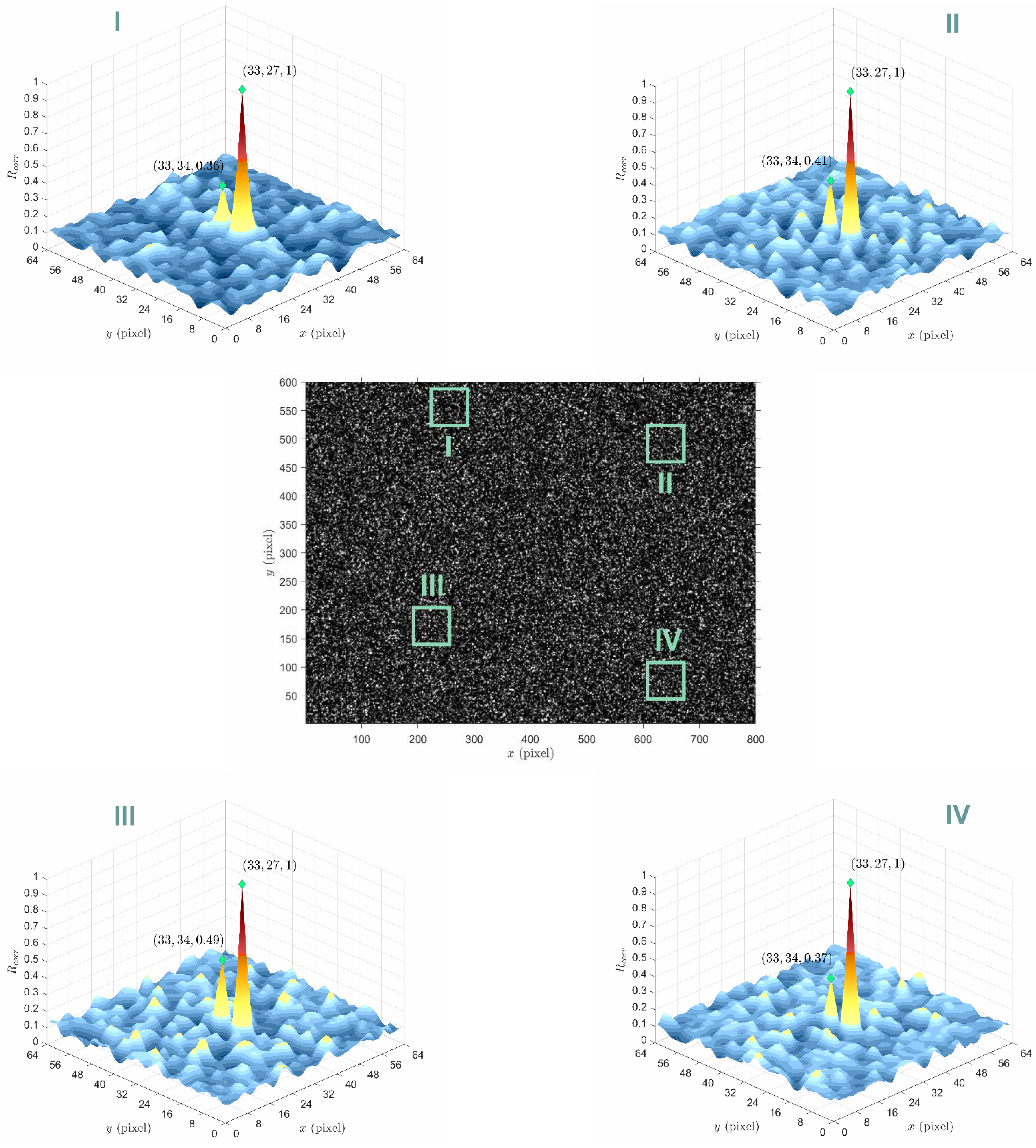
Particle image velocimetry (PIV) has been a sophisticated non-intrusive technique for quantifying gas or liquid flows for measuring either planar motion or three-dimensional movement [1]. Dividing consecutive image pairs into numerous interrogation windows, performing cross correlation, and locating in-plane displacements corresponding to the peak coefficient are the textbook routines in PIV analysis. Among the development and improvement of the PIV technique over the past decades, many efforts were made to figure out a perfect solution for accurately determining the correlation peak [1], particularly with the presence of strong in-plane displacement gradients [2] in which multiple prominent peaks may appear in a correlation coefficient map. However, this multi-peak coefficient map could provide a key to quantitatively describe stratified crossflows. A quick example is shown in Figure 1. The middle plot of Figure 1 is a snapshot representing an artificial stratified crossflow composite of two unidirectional flows—one constantly moves upward by two pixels and the other moves to the opposite way by a constant five pixels. Four random areas of 64 × 64 pixels were selected to calculate the normalized cross-correlation coefficient (Rcorr), and the resulting Rcorr maps are shown in the same figure. Interestingly, the two most prominent peaks correspond to the default planar displacements, and a consistent trend is found in all four Rcorr maps. This points out that both unidirectional flow fields are simultaneously measured, and potentially, they can be separated by the given Rcorr map. If a conventional operation is applied, only the most prominent peak remains, and the other unidirectional flow will be completely ignored. Now, the demonstration in Figure 1 intrigues the possibility of a new algorithm that is able to automatically identify the peaks corresponding to the flows in different directions. Multiple velocity fields can thus be revealed from stratified crossflows. More importantly, the flexibility to instrument deployment in either laboratory or field measurement would be largely gained if this new algorithm requires the images simultaneously acquired from a single field of view (FOV).
Speaking to the potential applications, this new algorithm may be readily applied to quantify complex atmospheric motions, especially the phenomenon of atmospheric stratification. Atmospheric stratification, induced by the descending cold air intrusion into a basin atmosphere [3] or the interaction between turbulent air current and dispersive pollutants [4] or topographic obstacles [5], could alter and disturb the river, coast, or ocean environment. Such a phenomenon can be visually captured by satellites with multi-band or specialized optical sensors [6,7]. Nowadays, deriving atmospheric motion vectors (AMVs) from infrared satellite images is relatively common [8,9]. Nevertheless, deriving multiple vectors from stratified atmospheric flows, to the authors’ knowledge, has not been attempted yet. It can be imagined that more quantitative information valuable to meteorological, hydrological, or oceanographic research can be attained if the concept stated in the previous paragraph is made possible for analyzing the images acquired by satellites.
In addition to meteorological research, stratification phenomena in an estuary [10] or between currents and breaking waves in a rip current [11] imaged by satellites or an unmanned aircraft system (UAS) may be quantified by the concept. In addition, stratification induced by submerged granular collapse [12] or a propagating wave interacting with a fluid of a different density [13] are often experimentally investigated at a relatively small scale, where a transparent sidewall is mostly available for photography. However, if an experiment has to be performed at a large scale or in a basin, a transparent sidewall may not be feasible. In this case, the new algorithm along with photography from a top view is more likely to successfully quantify the planar flow motions of stratified crossflows
The objective of this study is to propose a new algorithm for simultaneously quantifying multiple flow fields from stratified crossflows optically captured in a single field of view. Validation is performed on two scenarios: one is an artificial crossflow generated by synthetic images; and the other is a crossflow simulated by a U-shaped water channel. This paper is organized as follows: the algorithm will be first introduced, followed up by the brief of each experiment and the validation result. Subsequently, discussions on uncertainties, error reduction, spurious vector filtering, limitations, and suggestions for applications will be given. The final part will be the conclusions.
2. Algorithm
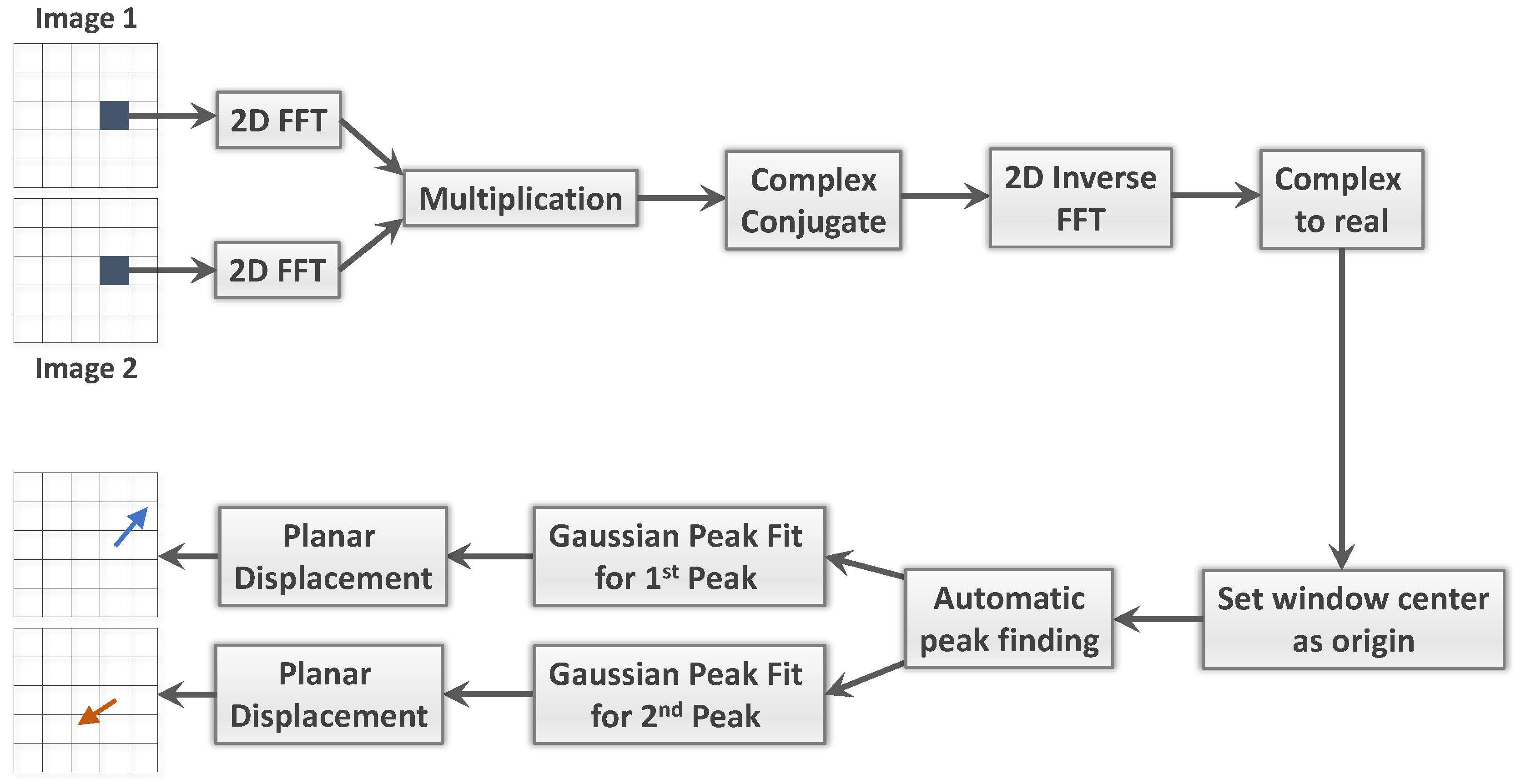
The concept of the new algorithm is implementing a new step right after the cross-correlation step; the full procedure is illustrated Figure 2. The entire procedure is similar to a PIV analysis routine that first adopts two consecutive images and divides each image into several square interrogation windows. Cross-correlation is then applied to the grayscale matrices of each image pair in each window for identifying the tracer displacement of maximum likelihood. The computation of discrete cross-correlation is very time consuming. To improve the computational efficiency, fast Fourier transform (FFT) is generally employed to the image matrices before performing cross correlation. By transferring to the frequency domain, a cross-correlation calculation can be simply done by the multiplication of coefficients, largely cutting down computation time. After setting zero frequency to the center of each window, the inverse FFT is employed to transfer the result back to the time domain, yielding a cross-correlation coefficient map. Then the identification of multiple prominent correlation peaks will follow up.
In a conventional PIV analysis routine, only the highest peak in the correlation map will be collected for determining the planar displacement. This is very straightforward in programming. For collecting multiple peaks in a two-dimensional domain full of local maxima, however, automatic peak finding becomes not trivial. A specific approach is required. In this study, an automatic peak finding scheme based on the concept of extrema is utilized. This scheme is initiated with the arrangement of a cross-correlation coefficient to be a two-dimensional matrix, , where subscripts i and j indicate the row element and column element, respectively. Then, collect the location (row number and column number) of local maxima along each row by the detecting condition:
The same operation is made through each column and diagonal in matrix , obtaining the location satisfying another detecting conditions:
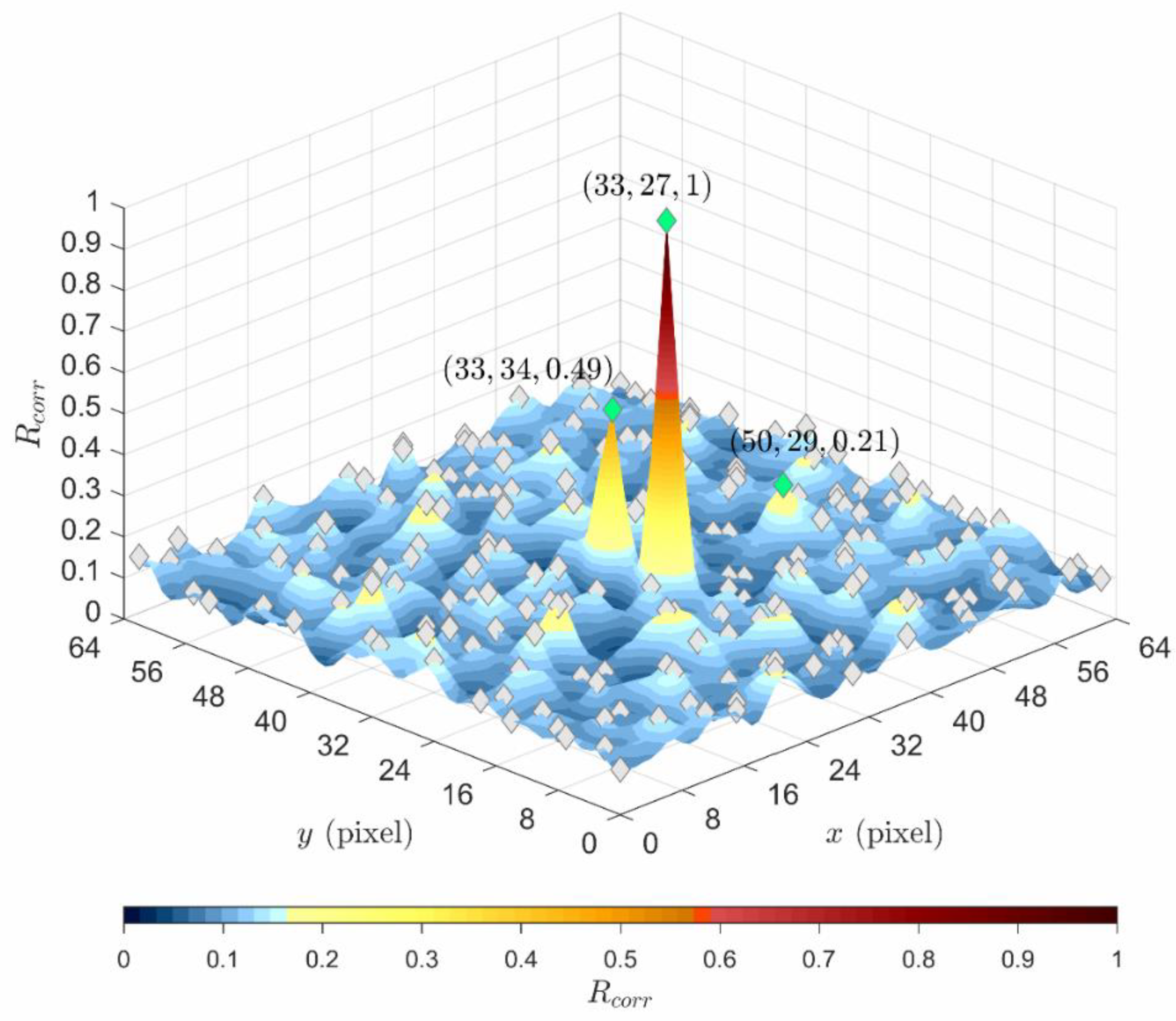
As a result, three sets of locations representing local maxima along row, column, and diagonal can be obtained. The final step is to take the intersection of these locations, yielding local Rcorr peaks in a two-dimensional domain. Figure 3 exhibits the product by applying the above-described automatic peak finding scheme to the upper-left Rcorr map in Figure 1. It can be seen that the first two peaks, corresponding to particles movement in two directions, are perfectly identified. It has to be noted that the number of the largest peaks to be collected depends on the number of dominant flows in the stratified crossflow of interest. The number can be obtained by visually inspecting the animation of recording images. The final step is using Gaussian peak fit [1] to approach each true peak. The merit of this scheme is in requiring no manual input and being fully automatic with great computational efficiency. This scheme is therefore applied as a sole peak finding scheme for searching the locations of multiple Rcorr peaks.
Similar to conventional PIV analysis, post-processing is generally required for removing or correcting spurious vectors from raw velocity fields. Standard deviation filters and median filters [1] are the most common and effective filtering schemes for the automatic detection and removal of spurious vectors. A standard deviation filter examines magnitude only, while a median filter evaluates both magnitude and direction. Preliminary tests on the stratified crossflows generated by both artificial and realistic image data suggest that a standard deviation filter is not necessary. Median filter is thus the sole filtering scheme in the present study.
For each target vector , the acceptable criterion for median filtering is given as:
where is an user-defined parameter. In the presentation of validation results, is chosen, leading to a narrower confidence level than the typical range of from 2 to 3. Reasons and a brief guidance will be elaborated in the Section 4. The search window is set to 3 × 3, which is a typical setting in PIV post-processing. To examine the validity of the new algorithm, no interpolation scheme and smoothing method are utilized in the following vector results presented.
3. Validation
The validation study was mainly carried out by comparing the velocity fields derived from stratified crossflows with ones derived from individual unidirectional flows, namely, the expected result. Two experiments were considered: one is the generation of a synthetic image representing simplified crossflow; and the other was done by constructing a specialized U-shaped water channel in which a crossflow can be visually captured from a lateral view. High-speed photography, artificial tracking particles, and illumination with d laser light sheets were implemented to acquire the image data. Each experiment will be briefly introduced below, followed up by validation result and short discussions.
3.1. Synthetic Crossflow
3.1.1. Synthetic Image Generation
Two synthetic particle image sets were first generated by the method built in the popular open-sourced PIV analysis software—PIVlab 2.38 [14]. One image set has uniform particle displacement moving downward with a constant displacement of five pixels. Similar particle image pattern but moving up was applied to the other set, with the displacement being set to four pixels. The tracking particle density in both image sets was set to 40%. The synthetic crossflow condition was then generated by the superposition of both synthetic particle image sets. Note that 101 consecutive frames were generated with additional seeding of random background noise. A snapshot of an image generated by the above-described approach as well as four example Rcorr maps of four randomly selected areas can be found in Figure 1.
3.1.2. Validation Result for Synthetic Image
Figure 4 presents the velocity maps determined by the 1st peak and 2nd peak derived from the proposed algorithm along with those derived by the conventional approach on unidirectional flows. In the comparison of instantaneous velocity maps (randomly selected from 100 data sets), not surprisingly, vectors corresponding to the 1st peak are fully resolved. Vectors corresponding to the 2nd peak are partially resolved. It is anticipated that not all vectors would be revealed since many effects, such as blocking, overlapping, or connecting of tracer image, may occur by random in space and time, leading to missing or erroneous vectors. Median filter works perfectly for such an analysis result. The resultant vectors, in terms of either magnitude or direction, are mostly expected, showing the applicability of the proposed algorithm. In Figure 4, the time-averaged velocity maps over all 100 data sets are presented as well. It can be seen that vectors corresponding to the 2nd peak are fully revealed, implying that the occurrence of missing or erroneous vectors could be temporally random. This inspires the immediate possibility of applying the new algorithm to steady or quasi-steady crossflow conditions, measuring full-field velocity fields with the consecutive images in a single field of view (FOV). Table 1 summarizes the root-mean-square errors (RMSEs) estimated from the time-averaged result. The RMSE in magnitude is on the order of 0.1 pixels, equivalent to the sub-pixel error with Gaussian peak fit [1]. That means a mere difference in terms of magnitude. For the RMSE in direction, the result of the 2nd peak has one order of magnitude larger than that of the 1st peak. Undesirable effects pointed out previously may mainly contribute to the error. In spite of that, the error at this level is quite acceptable.
3.2. Stratified Crossflow Fields in PIV Measurement
3.2.1. PIV Measurement Setup
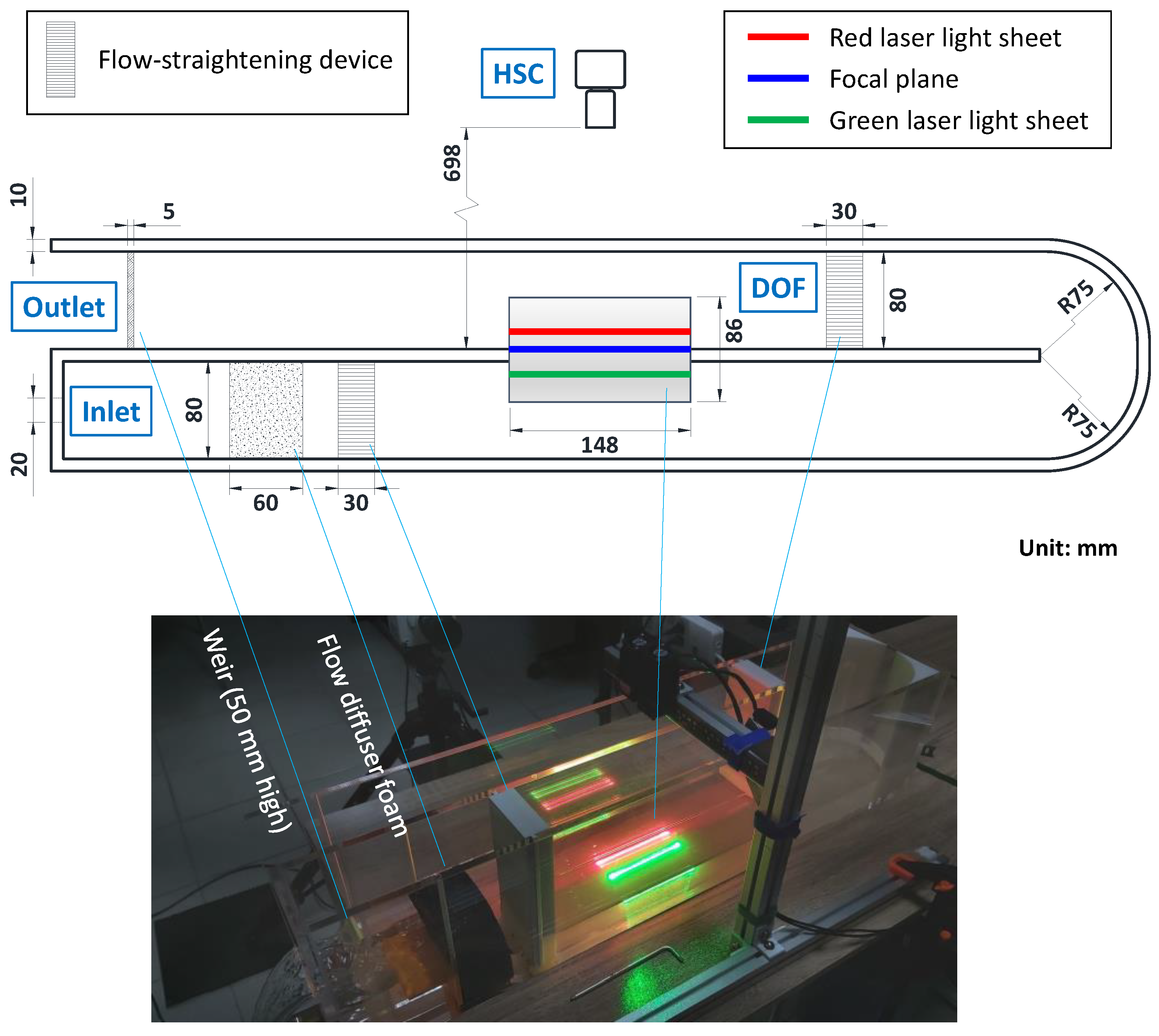
An open-circulated, U-shaped water channel made of acrylic plates, as shown in Figure 5, was constructed to generate a stratified crossflow condition in high-speed photography such that the proposed algorithm can be tested on a realistic fluid flow. As demonstrated in the top-view drawing and photo in Figure 5, the inflow goes rightward, and makes a U turn at the other end of the channel. Then the flow goes leftward all the way to the channel outlet. Flow straighteners were installed before the region of interest to ensure the flow uniformity. An additional flow diffuser foam was placed close to the inlet for mitigating the violent pipe inflow. Before the outlet, a weir of 50 mm high was installed for maintaining certain water level inside the channel.
In the present measurement, a high-speed camera (HSC), Phantom VEO 440, was placed to image the flows from a side view. If the DOF is sufficiently large, the HSC is supposed to capture the stratified crossflow-like pattern with one going rightward and the other going leftward, giving rise to an ideal condition for examining the validity of the new algorithm in the PIV measurement. Furthermore, to make the PIV measurement possible, the generation of two laser light sheets at appropriate locations is required for illuminating artificial seeding tracer. Figure 5 illustrates the implementation of two 100-mW continuous-wave (CW) laser sources as well as the locations of the light sheets. Note that there is no specific intension in using laser sources of different colors. In order to cover both laser light sheets, the DOF was set to 86 mm, with the f-number being set to 32 (largest). Note that Nikon AF Micro-Nikkor 60-mm lens was mounted. The focal plane was set to the middle wall surface of the water channel on the same side of the HSC. One thing that is inevitable is the influence of the acrylic plate. The media discontinuity more or less creates a discrepancy between the designed and real DOFs. Nevertheless, the present study tends to ignore this effect since its influence on velocity determination is observed not significant. Primary parameters in the high-speed photography are listed in Table 2.
Three image data sets were taken under different lighting conditions: only red laser on (case PIVR), only green laser on (case PIVG), and both red and green laser on (case PIVB). Each image data set was recorded for 10 s (2501 frames in total), with the frame rate being 1000 frames per second (fps). The image data in cases PIVR and PIVG were processed with a conventional PIV analysis routine, while the one in the case of PIVB was analyzed with the new algorithm. It should be marked that vectors derived from case PIVR and case PIVG serve the expected result.
3.2.2. Validation Result in PIV Measurement
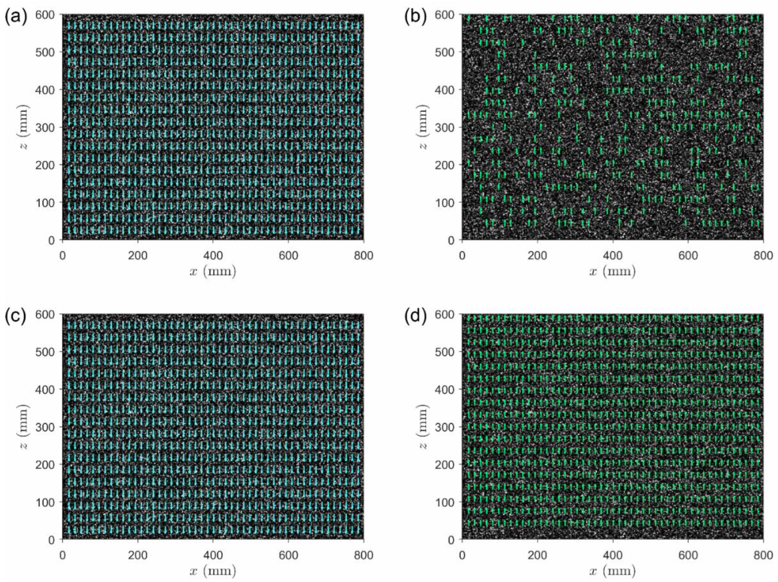
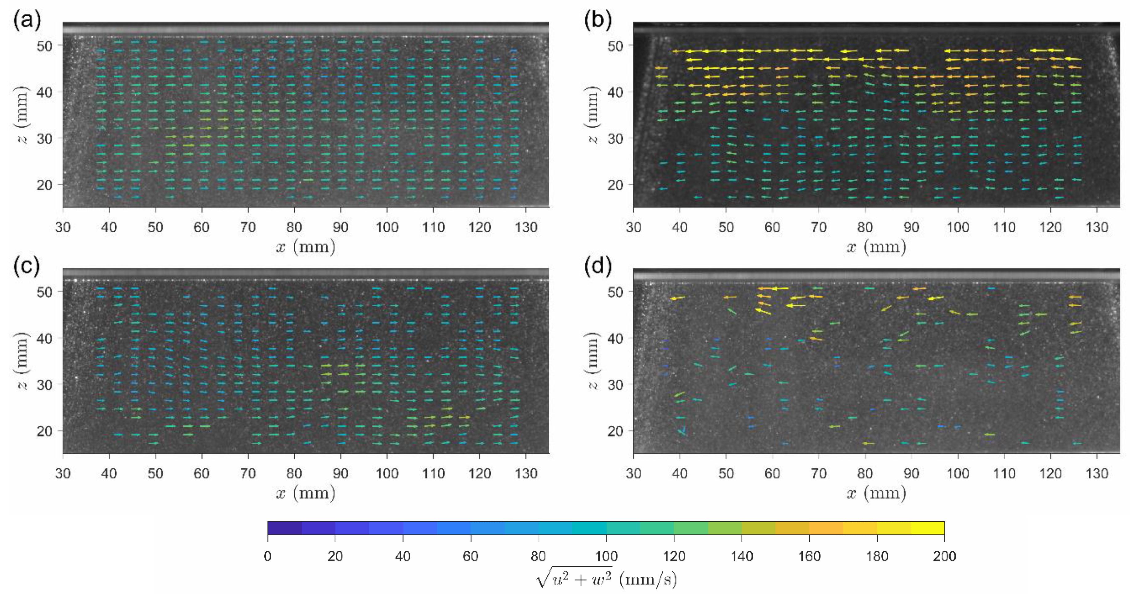
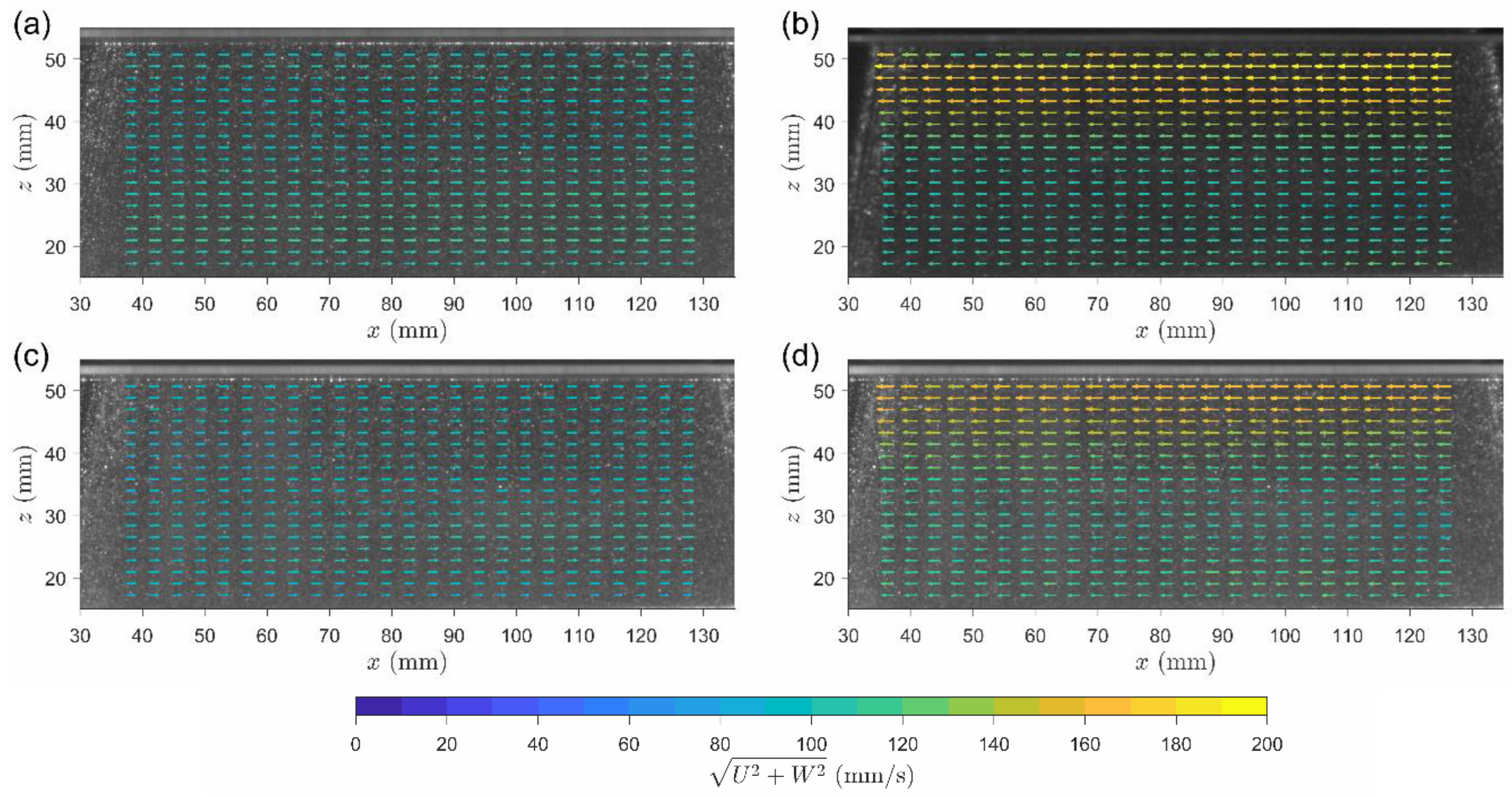
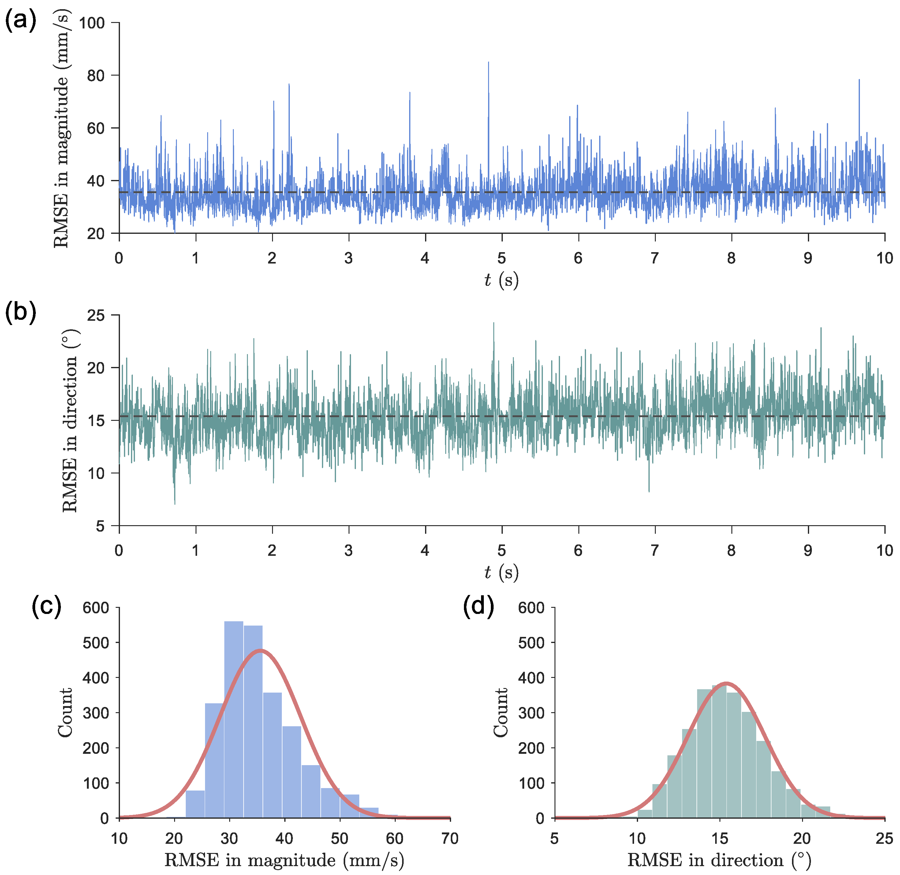
Figure 6 presents the instantaneous velocity maps determined by the 1st peak and the 2nd peak derived by the proposed algorithm from case PIVB along with those derived by the conventional procedure on unidirectional flows (cases PIVR and PIVG). It can be seen that the velocity maps corresponding to the 1st peak is similar to those in case PIVR, in which its laser sheet is closer to the HSC. In spite of lesser vectors revealed and more deflected vectors, the comparison is consistent with what was described in the validation result for synthetic images. It should be particularly mentioned that cheap CW laser sources were used in the present experiment. Therefore, the result is expected to be much improved if genuine lab-graded CW laser sources are utilized for shining light sheets. Figure 7 demonstrates the time-averaged velocity maps are over 2500 data sets. Not only are all vectors revealed, but the direction of most vectors agree with the expected result. Table 3 summarizes the RMSE estimation for the time-averaged result only. Note that the sub-pixel error is equivalent to 2.91 mm/s. The RMSE in magnitude corresponding to the 2nd peak is about three times of the sub-pixel error, within the acceptable range though. The RMSE in direction is acceptable as well. Surprisingly, the RMSE value in direction corresponding to the 1st peak is slightly larger, and the three-dimensional motion induced by the upstream condition of the turning flow may be the cause. Figure 8 further plots the time series of RMSEs in both magnitude and direction as well as their histograms with Gaussian fits for the vector result determined by the 2nd peak. This result consolidates the immediate applicability of the new algorithm to stratified crossflows since the discrepancy in magnitude and direction is random over time. Such a random error may be enormously reduced by time averaging or even ensemble averaging.
4. Discussions
Discussions on uncertainties, spurious vector filtering, error reduction, and limitations pertinent to the new algorithm are given in the following.
4.1. Uncertainties and Error Reduction
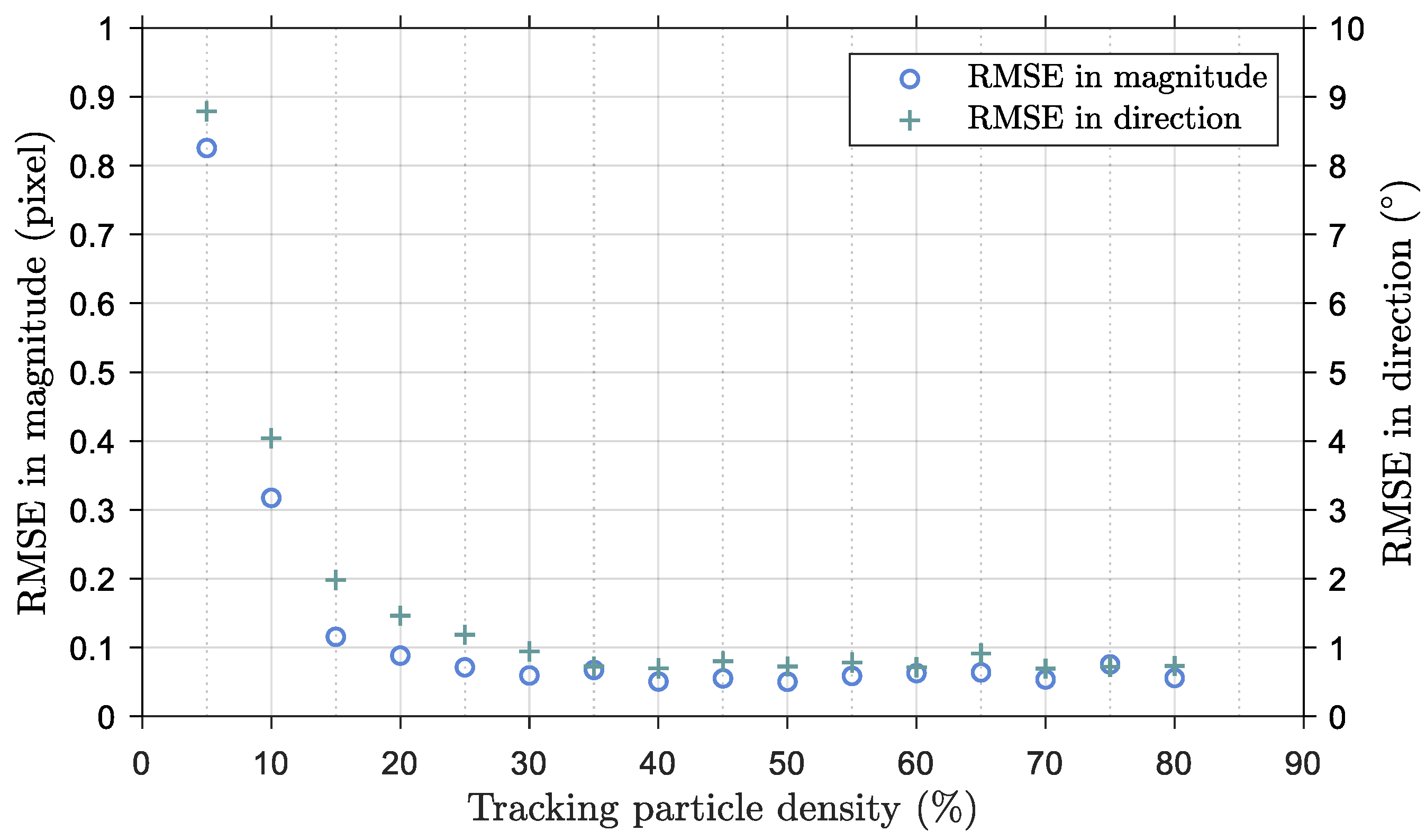
The recognition of a clear tracer image plays a critical role in the successful identification of multiple flow fields in stratified crossflows with their behaviors being optically captured. Among numerous factors, the illumination approach and tracer generation are crucial. The greater the contrast between the tracer image and the background noise, the higher the signal-to-noise ratio is that can be detected in favor of correlation peaks. Seeding artificial particles is a common tracer image generation approach in imaging-based velocimetry. To allow the identification of multiple flow fields and the inclusion of multiple laser light sheets with a single FOV, DOF has to be relatively deep. A deeper DOF would introduce a higher chance of visual blockage or a connected tracer image, and the density of the tracking particles thus becomes a concern. To address this concern, various tracking particle densities, from 5% to 80% with an interval of 5%, were tested with an artificially generated image, and the result is plotted in Figure 9. The test result shows that both RMSEs in magnitude and direction show an exponential decay against a higher tracking particle density. Intuitively, crowded tracking particles have a higher chance of blocking or getting connected to each other. However, the monotonic trend in Figure 9 implies that the errors in magnitude and direction are independent of the blockage or connection of the tracking particles at a high tracking particle density. Furthermore, to meet the sub-pixel accuracy, Figure 9 suggests the tracking particle density to be equal to or higher than 30%. In a typical PIV analysis, a low tracking particle density should be avoided since the target peak correlation coefficient may become less prominent due to the relatively low signal-to-noise ratio. The examination over the peak finding results reveals that the signal-to-noise ratio for the 2nd peak starts to decrease as the tracking particle density reaches lower than 30%. In other words, a lower tracking particle density would raise the possibility of finding the 2nd peak, which does not represent the flow. Nevertheless, it should be advised that the 30% threshold would be applicable to ideal artificial seedings. For non-ideal artificial seedings or natural seedings, a convergency test would be necessary for optimizing the tracking particle density.
A deeper DOF would be mostly considered for capturing a stratified crossflow for multiple flow field determination. In addition to the concern described previously, the larger geometric error () is another related to the spatial uncertainty in the direction normal to the FOV. For a uniform flow at a constant speed, for instance, the displacement derived from the tracking particles close to the farthest limit of the DOF would be larger than that at the focal plane where correct displacement is derived. This discrepancy is caused by the nature of lens projection and can be simply quantified by geometric similarity. Note that is calculated as , where is the distance from the lens’ focal point to the target focal plane. Any raw vector therefore suffers from such a spatial uncertainty or so-called geometric error. Fortunately, geometric error is in principle a random process over time. Based on the fact, time averaging is an ideal approach for minimizing with a reduction factor of N−0.5 or (N−1)−0.5 associated with sample or population standard deviation, where N is the number of data sets used in the averaging.
A clear tracer image of high contrast is much desired in enhancing the peak prominency in the correlation map associated with each flow component in a crossflow. This is considered the most effective measure of error reduction for raw vector result. Geometric error and random error, as described earlier, may be reduced by time averaging. In fact, if a given flow condition is repeatable with identical initial and boundary conditions, the velocity fluctuation among repetitions can be viewed as a random process as well. Consequently, the so-called ensemble averaging can be applied to those repetitions for obtaining mean flow quantities. The geometric error reduction is automatically achieved in ensemble averaging. In short, the longer the time averaging or the more repetitions in the ensemble averaging, multiple velocity fields with higher confidence would be obtained from a stratified crossflow with single FOV free of synchronization issue.
4.2. Spurious Vector Filtering
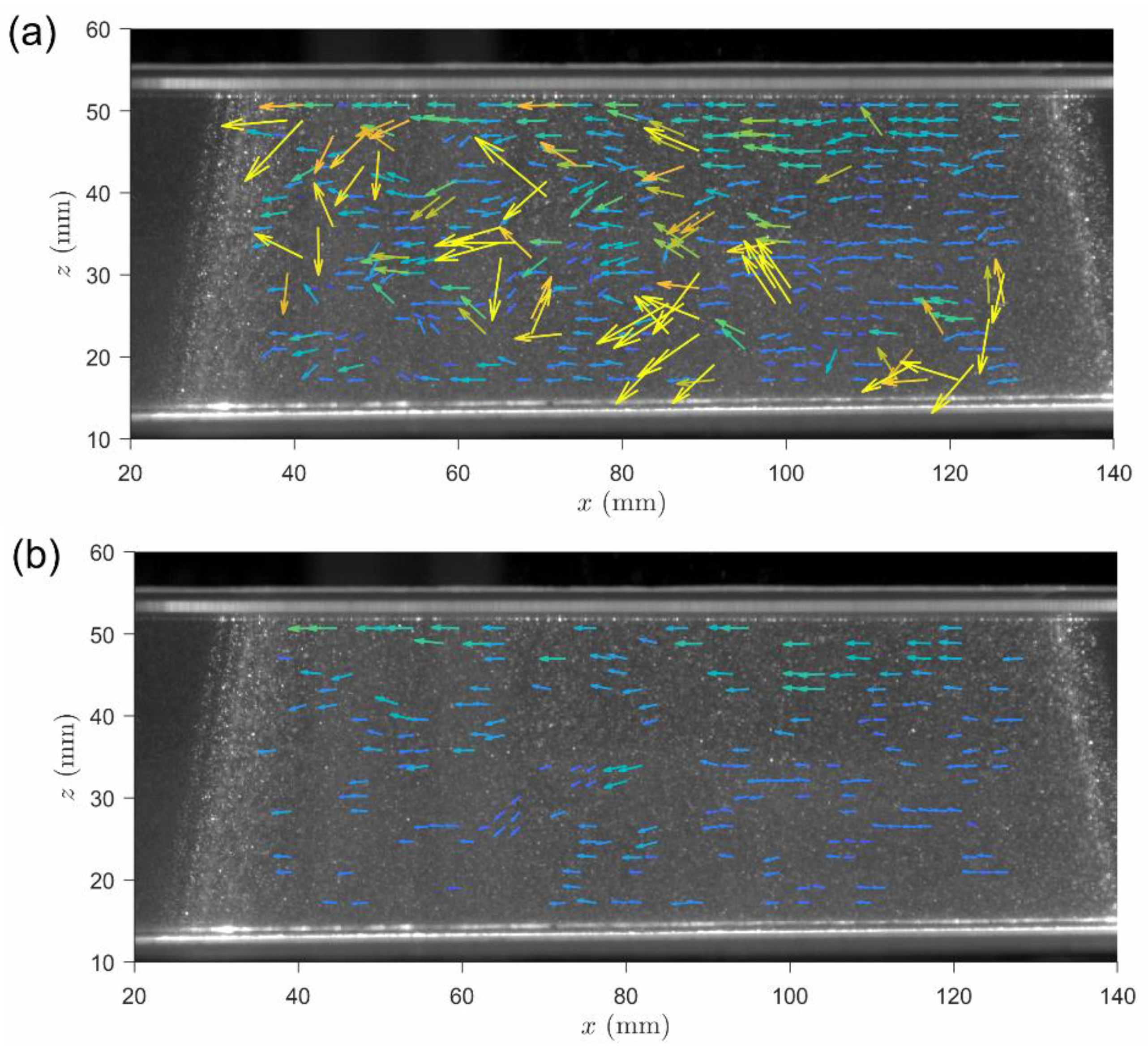
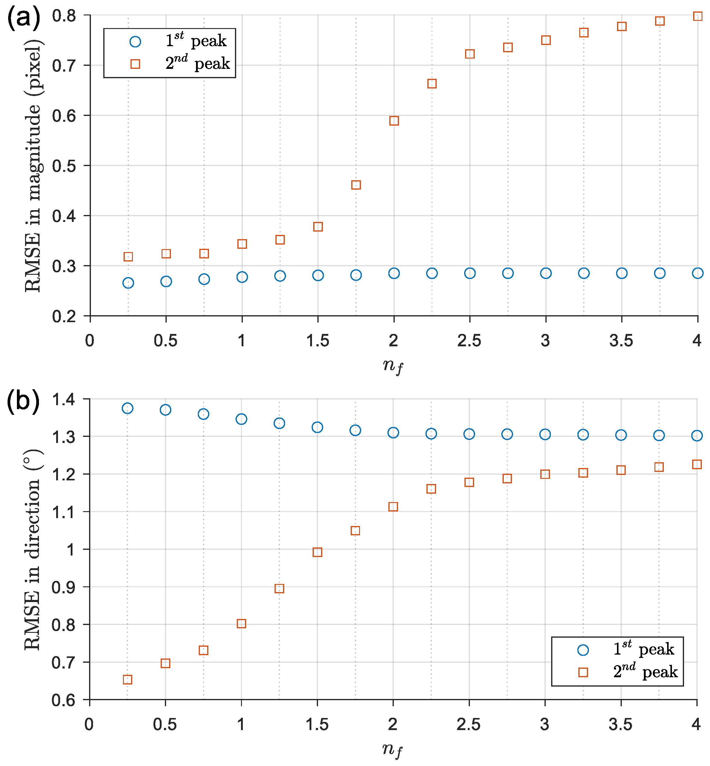
In the present study, a median filter is the sole filtering scheme adopted in the automatic spurious vector removal from the raw result derived by the new algorithm. This filtering condition is based on the continuity of magnitude and direction. There is only one use-defined parameter, , in the median filtering scheme as shown in Equations (4) and (5). For general PIV analysis, choosing the from 2 to 3 is a common practice to define the confidence level for acceptable vectors. As stated in Section 2, a narrower confidence level is set by choosing . This value is not randomly selected. Instead, this is mainly done by visual examination over the filtered velocity fields obtained from different . An ideal will have all spurious or erroneous removed. Every vector in the filtered result should not only satisfy the continuity requirement, but also match the motion of the corresponding tracking particles. Figure 10 presents a quick comparison between raw and filtered velocity maps with . It is very obvious that spurious or erroneous vectors are likely to be relatively large in magnitude and deviate more from the direction of dominant flow, indicating that visual examination is a reliable way. The same applies to all velocity maps over time. On the other hand, if any expected result, such as theoretical solution, numerical simulation, textbook criterion, or data measured by other techniques or instruments, is available, further steps must be taken to quantify the error and optimize the . Figure 11 demonstrates an instance by calculating the RMSEs in both magnitude and direction against different for the two velocity fields (corresponding to the 1st peak and the 2nd peak) derived from case PIVB. Note that the RMSE in magnitude is converted from mm/s into pixels on purpose, so the value can be readily compared to the size of interrogation window (16 by 16 pixels) and sub-pixel error. Seeing to Figure 11a, an abrupt gain of the RMSE in magnitude appears for . For , the value for the magnitude stays less than 0.35 pixels. This level is considered to be on the same order of the magnitude of sub-pixel error or 0.1 pixels. Three-dimensional flow motion, imperfect illumination setup, and uncontrollable measurement conditions, such as non-uniform tracer distribution, tracer blockage, or connected tracer, mainly account for the value additional to the sub-pixel error. In spite of that, 0.35 pixels is generally an accepted level for the error in magnitude for the final PIV analysis result. is therefore chosen. For the comparison shown in Figure 11b, the RMSEs in direction for both velocity fields among different are on the magnitude of 1°, which should be considered acceptable as well. A lower level of the error in direction in the 2nd peak result is not expected. As previously mentioned in Section 3.2.2, the upstream condition of turning flow may be the cause.
It has to be noted that is not limited to the range from 1 to 3, but a range to begin with examination trial. An appropriate is supposed to be capable of removing all spurious and erroneous vectors, and few correct vectors could be removed though. Quantitative comparison between the filtered and expected result is probably the best way to determine . However, for most flow measurements, the expected result tends to be unknown or difficult to estimate. Visual examination on the continuity of magnitude and direction of each vector relative to its neighbors is thus the more feasible approach. Furthermore, recursive filtering or other filter schemes may be utilized. More details on the related filtering schemes can be referenced to [1].
4.3. Limitations and Suggestions for Applications
As an extension of conventional PIV analysis, the planar measurement nature of the new algorithm has to be kept in mind whenever employing it for practical applications. The new algorithm may be utilized to quantify the stratified crossflows containing three-dimensional structures to some extent. To fully reveal quantitative three-dimensional flow motion, stereoscopic or tomographic PIV techniques [1] should be considered for this need.
One major advantage of the imaging-based velocimetry technique is the capability of measuring turbulent flows, deriving quantities, such as velocity fluctuation, turbulent kinetic energy dissipation, and so on. In order to evaluate those quantities, instantaneous full-field velocity fields must be known. The instantaneous flow fields corresponding to the 1st peak, as shown in Figure 6b,c, may meet the requirement if an appropriate interpolation method (cubic spline or Kriging) is adopted to fill the missing vectors removed by the filtering post-processing. However, the same may not be applicable to velocity fields corresponding to the peaks other than the 1st peak since more missing vectors appear. Most of those missing vectors are associated with the unfavorable correlation peak recognition caused by the blockage or connection of the tracer image. Figure 6d and Figure 10a,b serve as an excellent example for the description. In this case, the valid vectors are too sparse for the interpolation purpose with confidence. Therefore, the new algorithm is only possible to measure the turbulent stratified flow field corresponding to the 1st peak, but not the flow fields corresponding to other peaks. In spite of that, the new algorithm is still useful in obtaining further velocity information from turbulent or transient stratified crossflows, particularly in field measurements or large-scale experiments with more limitations in instrumentation. The velocity information corresponding to other peaks may fail to reveal the full quantitative flow structure but be able to provide valuable measured data for certain purposes, such as validation, indication, or observed input to data assimilation.
In regard to the measurement setup for the new algorithm, the experiment for an open channel flow in this study shows an approach for firing two laser sheets for illuminating the flow regions of interest as well as limiting the y position (normal to the measurement plane and FOV) of the obtained vectors. In this approach, the DOF has to be sufficiently deep, so all focal planes can be in-focus for achieving a higher signal-to-noise ratio in the cross-correlation result. Again, the deeper DOF would introduce a larger geometric error. As mentioned in Section 4.1, geometric error can be effectively reduced by time averaging and ensemble averaging.
Another specific flow region is the interface of stratified crossflows. For applying the new algorithm to measure such a region, a single light sheet provided by a laser or light-emitting diode (LED) with fine position control is preferred. In this setting, a shallower DOF with a depth similar to the width of the light sheet is suggested.
For the stratified crossflow measured by PIV in this study, all vectors pointing towards a positive x direction correspond to the 1st peak in the cross-correlation result, and others pointing towards a negative x direction correspond to the 2nd peak in the cross-correlation result. However, this may not always be the case for all kinds of applications, no matter whether single or multiple light sheets are utilized. If multiple light sheets are available, this issue may be solved by fine tuning the relative distances between the focal plane and each light sheet. Tracer images within the light sheet closer to the focal plane result in a higher cross-correlation peak. As a result, the dominant flow of each vector can be simply designated through the ranking of the correlation peaks. If multiple light sheets are not available or fine tuning is not possible, the alternative way can be done by first identifying the major directions of the dominant flows through visual inspection on the recorded images. Those directions are then set as indices in the further grouping procedure. However, the alternative may not work well if the directions are too similar. This is caused by the existence of velocity fluctuation in time and space. Future works are needed to tackle this difficulty. For now, the new algorithm is feasible for the stratified crossflows with component flows with a distinct difference in dominant directions. According to Figure 8b, a difference in direction larger than 10° is currently suggested.
Lastly, with clear tracer images representing each dominant flow motion, the new algorithm in principle works well for the stratified crossflows free of the above-mentioned limitations, no matter whether the flows are known or not. Nevertheless, future works are still needed for evaluating the applicability of the new algorithm in various fields of science and engineering.
5. Conclusions
A new imaging-based algorithm for deriving multiple velocity fields from stratified crossflows is presented. The new algorithm is similar to the conventional PIV analysis procedure except an additional automatic peak finding scheme is further implemented. Image data simultaneously acquired from a single FOV is only required, largely reducing the cost and complexity of instrumentation, and avoiding the synchronization issue especially at a high framing rate. A validation study was done with the stratified crossflows generated by synthetic and realistic images. For synthetic images, RMSE in magnitude from a time-averaged result is found to be equivalent to the sub-pixel error with a Gaussian peak fit in typical PIV analysis. The value gains up to three times in PIV measurement but is still acceptable for general purposes. RMSE in direction has a similar level in both validation results. Furthermore, the temporal distribution of both RMSE histograms in magnitude and direction are found to be close to Gaussian. This means, for practical applications, that a time-averaged or an ensemble-averaged result is recommended since the random error and geometric error would be greatly reduced, and more valid vectors in the region of interest would emerge. This implies that the new algorithm suits steady or quasi-steady flows or flows repeatable with identical initial and boundary conditions.
The examination on the tracking particle density exhibits that a higher density is preferred for reducing the RMSEs in both magnitude and direction. The present study found that the density equal to or higher than 30% is suggested. For selecting the confidence level in median filtering for removing spurious raw vectors, an example procedure was demonstrated. Owing to the combined factors on affecting the detection of clear tracer images, a higher chance of spurious or erroneous vectors, corresponding to the peaks other than the 1st one, is expected in the raw velocity fields. As a result, a narrower confidence level is preferred in median filtering herein. In regard to instrumentation, the multiple positions perpendicular to the FOV can be controlled by the illumination setting, ensuring that the position of each vector from a different velocity field is known. Details on the limitations and suggestions on the aspects of practical use of the new algorithm should be referred to discussions.
Author Contributions
Conceptualization, W.-L.C.; methodology, W.-L.C. and S.-M.L.; software, W.-L.C. and S.-M.L.; validation, W.-L.C. and S.-M.L.; formal analysis, W.-L.C. and S.-M.L.; investigation, W.-L.C. and S.-M.L.; resources, W.-L.C.; data curation, W.-L.C.; writing—original draft preparation, W.-L.C.; writing—review and editing, W.-L.C.; visualization, W.-L.C. and S.-M.L.; project administration, W.-L.C.; funding acquisition, W.-L.C. All authors have read and agreed to the published version of the manuscript.
Funding
This research was financially supported by the Ministry of Science and Technology, Taiwan, under grant MOST 110-2636-E-110-007 (MOST Young Scholar Fellowship Program).
Institutional Review Board Statement
Not applicable.
Informed Consent Statement
Not applicable.
Data Availability Statement
The data supporting the findings of this study are available on request from the corresponding author.
Acknowledgments
Authors would like to thank Cheng-Hsien Lee for providing CW laser devices, and Wan-Jo Chang for the help in conducting the experiment.
Conflicts of Interest
The authors declare no conflict of interest.
References
- Raffel, M.; Kähler, C.J.; Willert, C.E.; Wereley, S.T.; Scarano, F.; Kompenhans, J. Particle Image Velocimetry: A Practical Guide; Springer: Berlin/Heidelberg, Germany, 2018. [Google Scholar]
- Masullo, A.; Theunissen, R. On dealing with multiple correlation peaks in PIV. Exp. Fluids 2018, 59, 89. [Google Scholar] [CrossRef] [Green Version]
- Whiteman, C.D.; Lehner, M.; Hoch, S.W.; Adler, B.; Kalthoff, N.; Haiden, T. Katabatically Driven Cold Air Intrusions into a Basin Atmosphere. J. Appl. Meteorol. Clim. 2018, 57, 435–455. [Google Scholar] [CrossRef]
- Guo, D.P.; Zhao, P.; Yao, R.T.; Li, Y.P.; Hu, J.M.; Fan, D. Numerical and Wind Tunnel Simulation Studies of the Flow Field and Pollutant Diffusion around a Building under Neutral and Stable Atmospheric Stratifications. J. Appl. Meteorol. Clim. 2019, 58, 2405–2420. [Google Scholar] [CrossRef]
- Wang, Y.S.; MacCall, B.T.; Hocut, C.M.; Zeng, X.P.; Fernando, H.J.S. Simulation of stratified flows over a ridge using a lattice Boltzmann model. Environ. Fluid Mech. 2020, 20, 1333–1355. [Google Scholar] [CrossRef] [Green Version]
- Browning, K.A.; Clough, S.A.; Davitt, C.S.A.; Roberts, N.M.; Hewson, T.D.; Healey, P.G.W. Observations of the mesoscale sub-structure in the cold air of a developing frontal cyclone. Q. J. R. Meteorol. Soc. 1995, 121, 1229–1254. [Google Scholar] [CrossRef]
- Clerbaux, C.; Hadji-Lazaro, J.; Turquety, S.; George, M.; Boynard, A.; Pommier, M.; Safieddine, S.; Coheur, P.F.; Hurtmans, D.; Clarisse, L.; et al. Tracking pollutants from space: Eight years of IASI satellite observation. Comptes Rendus Geosci. 2015, 347, 134–144. [Google Scholar] [CrossRef]
- Velden, C.; Lewis, W.E.; Bresky, W.; Stettner, D.; Daniels, J.; Wanzong, S. Assimilation of high-resolution satellite-derived atmospheric motion vectors: Impact on HWRF forecasts of tropical cyclone track and intensity. Mon. Weather Rev. 2017, 145, 1107–1125. [Google Scholar] [CrossRef]
- Chuang, W.L.; Chou, C.B.; Chang, K.A.; Chang, Y.C.; Chin, H.L. Atmospheric Motion Vectors Derived from an Infrared Window Channel of a Geostationary Satellite Using Particle Image Velocimetry. J. Appl. Meteorol. Clim. 2019, 58, 199–211. [Google Scholar] [CrossRef]
- Garcia, A.M.P.; Geyer, W.R.; Randall, N. Exchange Flows in Tributary Creeks Enhance Dispersion by Tidal Trapping. Estuaries Coasts 2022, 45, 363–381. [Google Scholar] [CrossRef]
- Kim, H.D.; Kim, K.H. Analysis of Rip Current Characteristics Using Dye Tracking Method. Atmosphere 2021, 12, 719. [Google Scholar] [CrossRef]
- Lee, C.H.; Kuan, Y.H. Onset of submerged granular collapse in densely packed condition. Phys. Fluids 2021, 33, 121705. [Google Scholar] [CrossRef]
- Wu, H.L.; Hsiao, S.C.; Lin, T.C. Evolution of a two-layer fluid for solitary waves propagating over a submarine trench. Ocean Eng. 2015, 110, 36–50. [Google Scholar] [CrossRef]
- Thielicke, W.; Sonntag, R. Particle Image Velocimetry for MATLAB: Accuracy and enhanced algorithms in PIVlab. J. Open Res. Softw. 2021, 9, 12. [Google Scholar] [CrossRef]
Figure 1.
Normalized cross-correlation coefficient (Rcorr) maps of four randomly selected windows with a size of 64 × 64 pixels. Note that the central particle image represents a snapshot of a synthetic stratified crossflow composite of one unidirectional flow moving downward by constant 5 pixels and the other moving upward by constant 2 pixels.

Figure 2.
Procedure of the proposed algorithm.

Figure 3.
Diamond: Local peaks identified by the automatic peak finding scheme. Green diamond marks the peaks of the largest three Rcorr.
Figure 3.
Diamond: Local peaks identified by the automatic peak finding scheme. Green diamond marks the peaks of the largest three Rcorr.

Figure 4.
Plots in top panel are the instantaneous velocity maps corresponding to (a) 1st peak and (b) 2nd peak; and plots in bottom panel are the time-averaged velocity maps corresponding to the (c) 1st peak and (d) 2nd peak.
Figure 4.
Plots in top panel are the instantaneous velocity maps corresponding to (a) 1st peak and (b) 2nd peak; and plots in bottom panel are the time-averaged velocity maps corresponding to the (c) 1st peak and (d) 2nd peak.

Figure 5.
PIV setup for a stratified crossflow condition generated by a U-shaped channel. Top and bottom panels are the top-view drawing and photo of the experiment, respectively.
Figure 5.
PIV setup for a stratified crossflow condition generated by a U-shaped channel. Top and bottom panels are the top-view drawing and photo of the experiment, respectively.

Figure 6.
Instantaneous velocity maps determined by typical PIV analysis and the proposed algorithm. (a) case PIVR, (b) case PIVG, and result corresponding to the (c) 1st peak and (d) 2nd peak in case PIVB.
Figure 6.
Instantaneous velocity maps determined by typical PIV analysis and the proposed algorithm. (a) case PIVR, (b) case PIVG, and result corresponding to the (c) 1st peak and (d) 2nd peak in case PIVB.

Figure 7.
Time-averaged velocity maps determined by typical PIV analysis and the proposed algorithm. (a) case PIVR, (b) case PIVG, and result corresponding to the (c) 1st peak and (d) 2nd peak in case PIVB.
Figure 7.
Time-averaged velocity maps determined by typical PIV analysis and the proposed algorithm. (a) case PIVR, (b) case PIVG, and result corresponding to the (c) 1st peak and (d) 2nd peak in case PIVB.

Figure 8.
(a,b) are the time series of RMSE in magnitude and direction, respectively, for the vectors corresponding to 2nd peak in case PIVB, with dashed line being the mean value in each plot. (c,d) are the histogram plots of (a,b), respectively, with maroon curves being Gaussian fit.
Figure 8.
(a,b) are the time series of RMSE in magnitude and direction, respectively, for the vectors corresponding to 2nd peak in case PIVB, with dashed line being the mean value in each plot. (c,d) are the histogram plots of (a,b), respectively, with maroon curves being Gaussian fit.

Figure 9.
RMSEs in magnitude and direction against different tracking particle densities in a synthetic stratified crossflow.
Figure 9.
RMSEs in magnitude and direction against different tracking particle densities in a synthetic stratified crossflow.

Figure 10.
Randomly selected (a) raw and (b) filtered velocity maps corresponding to the 2nd peaks in the cross-correlation results derived from case PIVB.
Figure 10.
Randomly selected (a) raw and (b) filtered velocity maps corresponding to the 2nd peaks in the cross-correlation results derived from case PIVB.

Figure 11.
RMSE in (a) magnitude and (b) direction against different for the two velocity fields (corresponding to 1st peak and 2nd peak) derived from case PIVB. Note that the magnitude is converted from mm/s to pixel.
Figure 11.
RMSE in (a) magnitude and (b) direction against different for the two velocity fields (corresponding to 1st peak and 2nd peak) derived from case PIVB. Note that the magnitude is converted from mm/s to pixel.


Table 1.
Summary of expected value and RMSEs in magnitude and direction from the validation result with synthetic images. Note that time-averaged results are used in error estimation.
Table 1.
Summary of expected value and RMSEs in magnitude and direction from the validation result with synthetic images. Note that time-averaged results are used in error estimation.
| Magnitude (Pixel) | Direction (Degree) | |||
|---|---|---|---|---|
| 1st Peak | 2nd Peak | 1st Peak | 2nd Peak | |
| Expected | 5 | 4 | −90 | 90 |
| RMSE | 0.04 | 0.05 | 0.06 | 0.70 |
Table 2.
Summary of primary parameters in the high-speed photography for PIV measurement.
| Resolution (Pixels) | Field of View (FOV) Size (mm2) | DOF (mm) | Distance-to-Focal Plane (mm) | Frame Rate (fps) |
|---|---|---|---|---|
| 1280 × 800 | 148 × 69 | 86 | 698 | 258 |
Table 3.
Summary of mean value and RMSEs in magnitude and direction from the validation result in PIV measurement. Note that time-averaged data are used to generate these values, and mean magnitude and direction are estimated from case PIVR (corresponding to 1st peak) and case PIVG (corresponding to 2nd peak).
| Magnitude (mm/s) | Direction (mm/s) | |||
|---|---|---|---|---|
| 1st Peak | 2nd Peak | 1st Peak | 2nd Peak | |
| Expected | 86.93 | 106.75 | 0.16 | 179.61 |
| RMSE | 8.06 | 9.98 | 1.35 | 0.80 |
Publisher’s Note: MDPI stays neutral with regard to jurisdictional claims in published maps and institutional affiliations. |
© 2022 by the authors. Licensee MDPI, Basel, Switzerland. This article is an open access article distributed under the terms and conditions of the Creative Commons Attribution (CC BY) license (https://creativecommons.org/licenses/by/4.0/).
Share and Cite
MDPI and ACS Style
Chuang, W.-L.; Lin, S.-M. A PIV-Based Algorithm for Simultaneous Determination of Multiple Velocity Fields from Stratified Crossflows in Single Field of View. Water 2022, 14, 1877. https://0-doi-org.brum.beds.ac.uk/10.3390/w14121877
AMA Style
Chuang W-L, Lin S-M. A PIV-Based Algorithm for Simultaneous Determination of Multiple Velocity Fields from Stratified Crossflows in Single Field of View. Water. 2022; 14(12):1877. https://0-doi-org.brum.beds.ac.uk/10.3390/w14121877
Chicago/Turabian StyleChuang, Wei-Liang, and Sheng-Mei Lin. 2022. "A PIV-Based Algorithm for Simultaneous Determination of Multiple Velocity Fields from Stratified Crossflows in Single Field of View" Water 14, no. 12: 1877. https://0-doi-org.brum.beds.ac.uk/10.3390/w14121877
Note that from the first issue of 2016, this journal uses article numbers instead of page numbers. See further details here.