

CN-N: A Python-based ArcGIS Tool for Generating SCS Curve Number and Manning’s Roughness

Stantec Consulting Services Inc., 6080 Tennyson Pkwy Ste 200, Plano, TX 75024, USA
*
Author to whom correspondence should be addressed.
Water 2023, 15(20), 3581; https://0-doi-org.brum.beds.ac.uk/10.3390/w15203581
Submission received: 21 September 2023
/
Revised: 8 October 2023
/
Accepted: 11 October 2023
/
Published: 13 October 2023
(This article belongs to the Special Issue Hydroinformatic Tools and Spatial Analysis in Water Resources and Water Extreme Events Study)
Abstract
:Water resources engineers and geospatial analysts often face the challenge of spatially estimating parameters such as the Soil Conservation Service (SCS) Curve Number (CN) and Manning’s roughness number (n), which are critical for predicting runoff and streamflow in hydrologic studies. Addressing the above challenge, this paper presents an innovative ArcMap tool developed using Python. This tool streamlines the SCS-CN and Manning’s n spatial calculations and is designed to handle large datasets, even at the scale of the entire US. Additionally, it offers the unique capability of geoprocessing mixed soil types and seamlessly integrating data if the watershed spans over different states. Our tool automates the integration of land cover data, hydrologic soil group data, and hydrologic boundaries. The tool reads watershed boundaries and uses the National Land Cover Database (NLCD) and the Gridded Soil Survey Geographic Database (gSSURGO) to develop SCS-CN and Manning’s n spatial layers. The tool also offers users the unique flexibility to add any desired values for CN or Manning’s n in the form of a so-called lookup table, which is a great help with the iterative process of calibrating hydrologic or hydraulic models. Our tool addressed one of the major limitations of its predecessors, acknowledging the existence of mixed hydrologic soil groups, e.g., B/C or C/D, and allowing for user adjustments to address hydrologic or hydraulic models’ calibration needs. The tool was developed with a flexible framework to incorporate additional spatial parameters soon, such as the spatial green-ampt parameters. With a user-friendly interface and integration capabilities, the tool is invaluable for hydrologic and hydraulic studies at local, regional, and global scales.
1. Introduction
Prediction of runoff within a reasonable uncertainty range plays a pivotal role in hydrologic studies, watershed management, and environmental risk assessments. Two significant parameters that heavily influence these predictions are the Soil Conservation Service (SCS) Curve Number (CN) and Manning’s roughness coefficient (n). The SCS-CN method, developed by the United States Department of Agriculture (USDA) Natural Resources Conservation Service (NRCS), is a simple empirical approach used for estimating direct runoff volume from a rainfall event in a catchment [1]. Manning’s n, an empirical roughness coefficient, is a critical component in open channel flow calculations, representing how fast streamflow can move over natural terrain with various land cover types [2].
Numerous studies have explored methods for estimating either CN or Manning’s n. The CN values are usually derived from land cover and hydrologic soil group data, as documented in the NRCS National Engineering Handbook [3]. Prior research efforts have indicated that land cover data from the National Land Cover Database (NLCD) can be successfully used for estimating CN [4]. However, calculating CN also requires an understanding of the hydrologic soil group, which has led to the creation of numerous lookup tables correlating the NLCD grid codes of land cover types with hydrologic soil group data [5,6]. Regarding Manning’s n, various studies have focused on assigning a reliable range of values to diverse groups of land cover classes and streambed compositions [7,8].
In the realm of Geographic Information Systems (GIS), various toolboxes have been designed to assist with the spatial assignment of CN and Manning’s n. For instance, the SCS-CN tool was developed to calculate curve numbers within ArcMap [9]. While these tools can be quite useful, they typically focus on a single parameter, potentially lacking comprehensive functionality or offering limited customization options. Previous tools developed in this domain had several notable limitations, which our work seeks to overcome. Primarily, many of these tools had fixed lookup tables, not offering any user input. They were restricted to using values solely based on the developers’ judgment, without the flexibility to adjust them based on updated datasets or model calibration needs. Another significant limitation was the reliance on small-scale data, particularly the SSURGO web soil data. With SSURGOs inherent spatial limitation for areas up to 100,000 acres, this spatial limitation is a great challenge for large-scale project domains. Additionally, existing tools often struggle with mixed hydrologic soil group types, e.g., B/C or C/D, limiting their utility in basins with diverse hydrologic soil groups.
To move toward a more comprehensive tool, we focused on an integrated approach for estimating both CN and Manning’s roughness n within a user-friendly GIS interface. Depending on the needs of projects, the tool has evolved since its initial release within the Stantec community. For instance, a certain version of the tool was specifically designed to work with the USGS Hydrologic Unit Code 10 boundaries (HUC10). The most recent version of the tool concurrently computes the SCS-CN and Manning’s n, incorporating land cover data from the NLCD, hydrologic soil groups from the USDA Gridded Soil Survey Geographic database (gSSURGO), and random hydrologic boundaries data. The tool generates detailed outputs for an exact watershed boundary or a user-specified buffer zone.
The tool offers the flexibility for users to input their own CN and n values and adjust as needed or utilize the default values in the absence of a custom table. Additionally, it provides the functionality to generate a template table for user review. As such, this tool represents a significant advancement in the simplification and automation of CN and Manning’s n calculations, ensuring a consistent and streamlined approach to this important step in setting up a hydrologic or hydraulic model. This multi-faceted functionality sets our tool apart from preceding tools, effectively bridging the divide between hydrologic modeling and geospatial analysis. The tool was developed dynamically in order to easily accommodate updates on national and global-scale projects. The following sections elaborate on how the tool works and show its application in a real-world engineering project.
2. Materials and Methods
The tool was developed using the internal Python module in ArcMap, with no need to install any extra software or packages. It was designed to work with the ArcMap environment but can be adapted for ArcGIS Pro with minor adjustments. The methodology used to develop the tool encompasses three levels, including data acquisition, data processing, and output generation.
2.1. Data Acquisition
The tool requires land cover and hydrologic soil group spatial information as input parameters. The land cover data are obtained from the Multi-Resolution Land Characteristics (MRLC) Consortium (https://www.mrlc.gov/ accessed on 10 July 2023), which hosts NLCD data. The NLCD provides 30.0 m, or about 90.0 ft, of land cover data for the United States with a 20-class legend modified from the previous Anderson Land Cover Classification System. The user is advised to use the most recent version available (as of now, 2019). The data update frequency is every five years.
For regions outside of the United States, land cover data can be acquired from the Land Cover Viewer (LCV) webpage (https://lcviewer.vito.be/download, accessed on 10 July 2023), provided by the Global component of the Copernicus Land Monitoring Service. The database provides 100 m resolution global land cover data for 2019 with a 20-class legend. However, the user should note that NLCD “ID Codes," representing distinct land cover classes, are different for the MRLC database from LCV, and these ID Codes must be adjusted accordingly for compatibility. Currently, the data are available for 2015 through 2019, with an update frequency of every year. Other data sources are available from which global land cover information can be extracted, e.g., WorldCover with 2020 and 2021 land cover data at 10 m resolution with 11-class legend (https://viewer.esa-worldcover.org/worldcover/, accessed on 10 July 2023).
Hydrologic soil data for each state within the US is sourced from the gSSURGO database (https://www.nrcs.usda.gov/resources/data-and-reports/gridded-soil-survey-geographic-gssurgo-database and https://nrcs.app.box.com/v/soils/folder/180112652169, accessed on 10 July 2023). This approach bypasses the limitations of the Web Soil Survey online webtool, which restricts the basin area to less than 100,000 acres, a threshold often exceeded by the spatial extent of interest. The database provides 10 m resolution soil data at the state level, with a data update frequency of every year.
For regions outside of the United States, HSG can be accessed through the EarthData webpage (https://daac.ornl.gov/SOILS/guides/Global_Hydrologic_Soil_Group.html, accessed on 10 July 2023). The database provides 250 m resolution HSG data, with the latest update released in 2020.
2.2. Data Processing
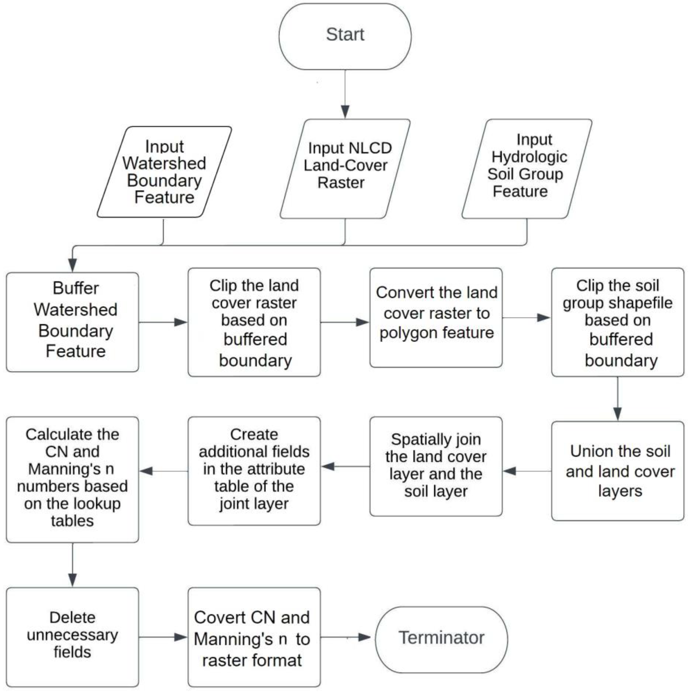
The tool initiates by creating a Geodatabase (GDB) within the assigned output folder. The input watershed boundary is then buffered (optional), and the land cover raster file is tailored according to this customized boundary. The idea of adding an optional buffer distance to the input boundary extent comes from the fact that geoprocessing a raster layer within an exact boundary usually leaves no-data or empty cells at the perimeter, which is not in the best interest of gridded-based hydrologic or hydraulic simulations.
The tool reads the land cover raster dataset and clips it using the buffered watershed boundary, resulting in clipped land cover raster data. Then, the tool clips the MUPOLYGON layer from the gSSURGO geodatabase using the buffered boundary. Next, the tool performs a “join” operation with the muaggatt table to incorporate hydrologic soil group data into the attribute table. The resulting data are copied to a new field, followed by the removal of the joined tables and the creation of a new soil layer. Subsequently, the polygonized land cover feature will be combined with the soil layer using “union” and “spatial join” operations. The tool applies either the user-provided table or the default table to compute CN and Manning’s n coefficients, generating an output feature with additional fields such as NLCD, HSG, description, abstraction ratio, and minimum infiltration ratio. The references for developing lookup tables are included in the tool to further educate users. Figure 1 illustrates the flowchart detailing the procedural steps of the tool.
3. Tool Interface and User Inputs
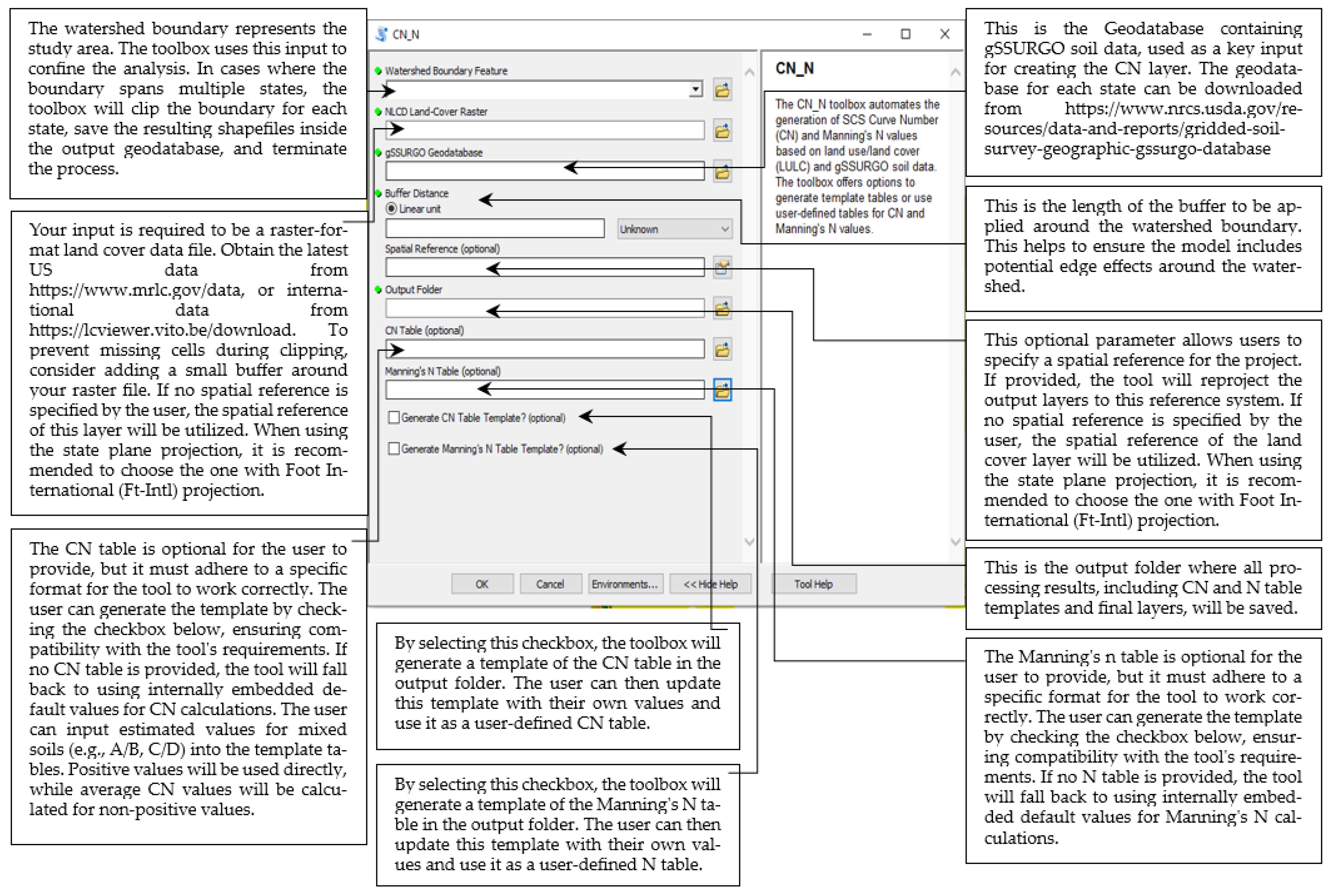
To enhance user understanding of the tool, we present an illustrative screenshot of the tool interface (Figure 2). The interface is designed with a focus on user friendliness and ease of understanding. To avoid referring the user to lengthy technical guides, informative notes will appear on the right ribbon while the user activates each input parameter section. The requirements for a successful tool operation can be summarized as follows:
3.1. Watershed Boundary Feature
The tool requires the user to input a shapefile representing the watershed boundary. It is advisable to utilize a dissolved boundary shapefile that encapsulates the entirety of the watershed boundary for optimal results. Regarding the State Plane coordinate system, users are advised to use the “FT-Intl” projection to avoid potential errors during the tool execution process.
3.2. NLCD Land Cover Raster
The user must input land cover data in raster format. As NLCD spatial data layers are typically large in file size, the user is advised not to upload the original NLCD raster files covering significantly large areas, such as an entire state or the entirety of the U.S. It is recommended to clip the original NLCD file to a smaller extent, then add the layer to the tool. It greatly helps with reducing the computational cost and processing time.
3.3. gSSURGO Soil Geodatabase
The user needs to provide the geodatabase containing the necessary soil data. The gSSURGO geodatabase should not be modified or disturbed by users. If the watershed spans over multiple states, the tool will automatically detect it and clip the watershed boundary for each state. The clipped boundaries will be saved inside the geodatabase in the output folder, and an error message will be displayed. In such cases, the user should run the tool again for each state separately, using the corresponding clipped boundary retuned by the tool and the state-specific gSSURGO geodatabase.
3.4. Buffer Distance
The user is required to input the desired buffer distance around the watershed boundary feature. This is to ensure that there are no null or missing values left in the output data at the perimeter, thus maintaining data integrity. The buffer option ensures data coverage of areas located at the border or perimeter, especially for gridded-based hydrologic and hydraulic simulations where software programs such as HEC-HMS 4.10 or HEC-RAS 6.0 return errors for missing spatial data at the boundary regions. However, the user is advised to avoid excessively large buffers due to computational cost; a range of 100 feet/m to a mile/km would be reasonable depending on the data resolution and purpose of analysis.
3.5. Spatial Reference
This field is optional, and it offers users the flexibility to specify a preferred output coordinate system. For watersheds spanning relatively smaller areas, adopting the state plane projection is recommended. However, if the user leaves the field blank, the tool will default to using the coordinate system of the LULC layer as the standard output coordinate system.
3.6. Output Folder
Specify the location where the output files should be stored. A geodatabase (gdb) will be automatically created within this folder, and all the generated files will be saved inside the geodatabase. The output layers can be exported from the geodatabase to any desired shapefile or raster layer format.
3.7. CN Table
The user has the option to provide a custom CN table. However, the table must strictly adhere to a specific format, including columns for NLCD, Dscr (description), and columns A to D, as well as all possible combinations to represent the mixed hydrologic soil groups. It is recommended that the user check the box in the tool interface to generate the CN table template, update it as needed, and upload it back to the tool. If no table is provided, the tool will utilize the default lookup table for calculations.
3.8. Manning’s n Table
Similar to the CN table, the user has the option to provide a customized Manning’s n table. The table must adhere to a specific format, and it is recommended to check the box to generate the n table template, update it accordingly, and upload it back to the tool. If no table is provided, the tool will utilize the default lookup table for Manning’s n calculations.
3.9. Generate CN Table Template
By selecting the appropriate box, the tool will create a template of the CN table in the output folder. This template can be updated by the user for future analysis. If the user prefers to input their own CN table, it is recommended to either update the generated template or ensure that the user-defined table has identical column names as the template.
3.10. Generate Manning’s n Table Template
By selecting the appropriate box, the tool will create a template of Manning’s n table in the output folder. The template can be updated by the user with their own values or used as a reference for creating a customized Manning’s n table. It is recommended to check this option when the user wants to provide their own Manning’s n values or modify the default template. The careful construction of user inputs, as detailed above, ensures the successful and efficient operation of the tool.
3.11. Lookup Tables and Parameter Determination
The tool utilizes three lookup tables to establish the relationships and calculations required for developing the CN and Manning’s n geospatial layers. These tables associate crucial parameters with specific land cover classes, serving as default values in the absence of user-provided tables. By referencing these lookup tables, the tool generates the CN and Manning’s n as initial estimates for the hydrologic or hydraulic modeling process.
3.12. NLCD Grid Code and Hydrologic Soil Group (HSG) Relationship
The first lookup Table 1 correlates each NLCD grid code with the CN assigned to each HSG. The NLCD grid code represents a unique land cover class, and the HSG represents the hydrologic characteristics of the soil. HSG Type A is assigned to soils with a high infiltration rate and lower potentials for generating runoff, while HSG Type D represents soils with a low infiltration rate and high runoff potentials. It should be noted that the CN values assigned to each grid code and HSG can be modified based on the geographical location of a project, updates in hydrologic guidelines, or evaluating the sensitivity of model outputs to initial assumptions made for CN.
3.13. NLCD Grid Code and Manning’s n Assignment
The second lookup Table 2 is utilized for Manning’s n assignment to each land cover class. This table links each NLCD grid code with a reasonable range of Manning’s n values. By presenting this range, the table informs the user on how Manning’s n can vary for each land cover class, while the tool adopts a normal n value for hydrologic and hydraulic analyses. It should be noted that the viable range provided in the lookup table is helpful to the user to select other Manning’s n values besides the suggested normal, if needed.
3.14. Infiltration Rates for Each Hydrologic Soil Group
The tool incorporates a predefined table that outlines the range of infiltration rates for each soil group (A, B, C, and D) (Table 3). These rates represent the volume of water absorbed by the soil column and play a crucial role in estimating runoff. The tool utilizes the minimum loss rate from the provided range for each soil group, ensuring a conservative estimate. It should be noted that the tool does not currently support user-uploaded tables for infiltration rates, and the default values embedded in the code are used. Additionally, in cases where mixed soils are present, the tool calculates the average infiltration rate for the combined soil groups. Other perspectives on how to handle mixed soil groups, e.g., A/C or A/D, can be accommodated within the tool.
3.15. Output Generation
Once the tool has completed the calculations for CN, Manning’s n, minimum infiltration rate, and abstraction ratio, it removes any extra fields from the attribute table. The resulting layer is then saved within the geodatabase located in the user-defined output folder. Additionally, the tool converts the Manning’s n layer into raster format in case the user is interested in utilizing the gridded Manning’s n layer for modeling purposes. Finally, any intermediate files within the geodatabase are deleted to ensure a clean and organized output.
4. Case Study
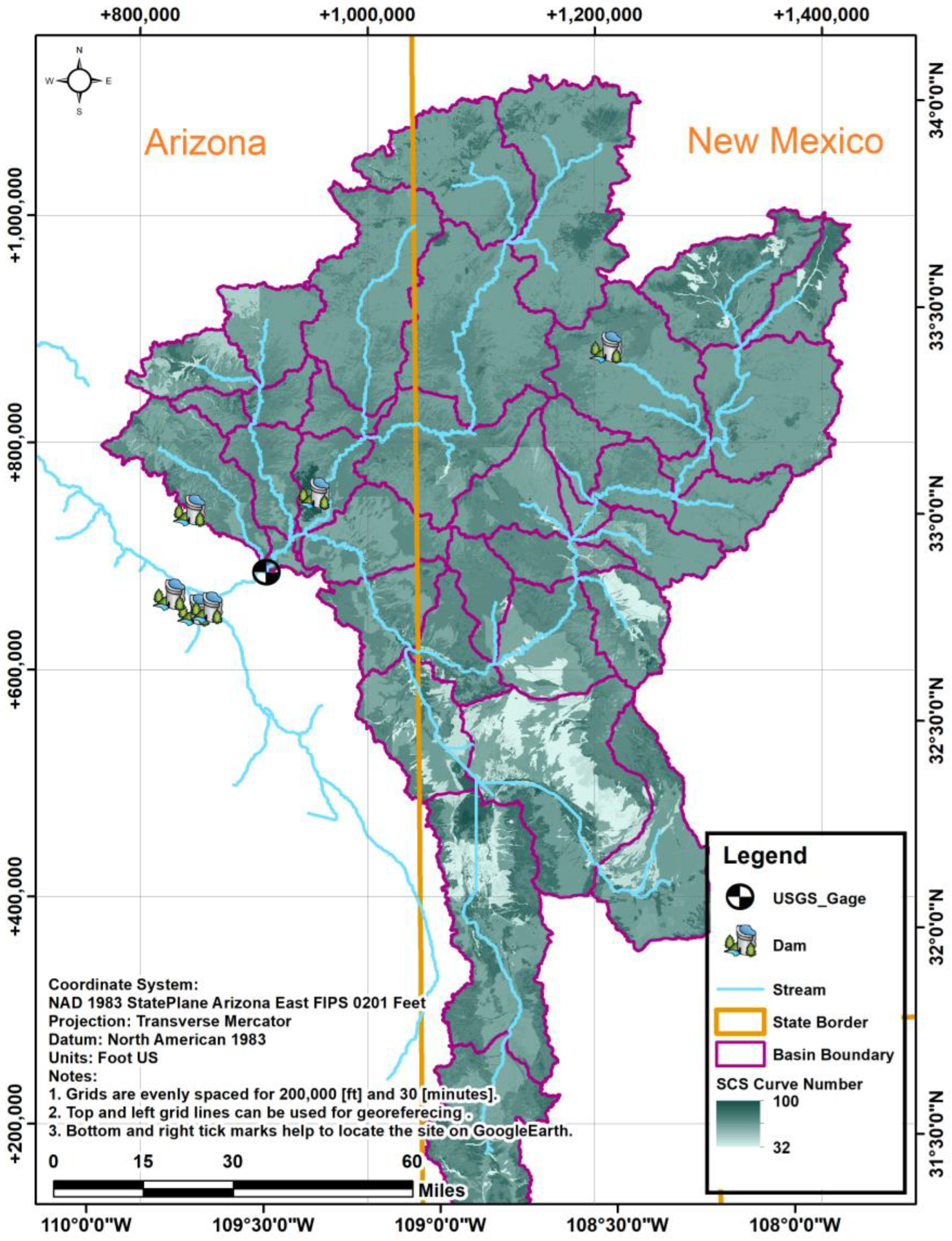
In this section, we review the performance of our tool in deriving CN and Manning’s n layers through a comprehensive case study. The chosen watershed, spanning over both New Mexico and Arizona, encompasses an extensive area of approximately 10,228 square miles. By harnessing 30 ft resolution topographic data, the watershed was delineated into several distinct sub-basins. Concurrently, streams were systematically identified utilizing the ArcHydro tool within the ArcGIS environment.
The 2019 land cover data were adopted from the NLCD database. The HSG data were obtained from USDA gSSURGO geodatabases for both New Mexico and Arizona. These databases were subsequently clipped to the region of interest and eventually merged to create a unified CN and Manning’s n layers. The choice of this watershed extent was intentional due to a number of factors. First, almost 53% of the watershed had no HSG data, which required user intervention in assuming reasonable HSG for no-data regions. Second, the watershed spans over two states, showcasing the tool’s capability to operate across state boundaries. Finally, the spatial extent of the watershed surpassed the limitations of the Web Soil Survey online webtool (basin area to be less than 100,000 acres or about 156 square miles) and required the direct usage of state-specific gSSURGO geodatabase.
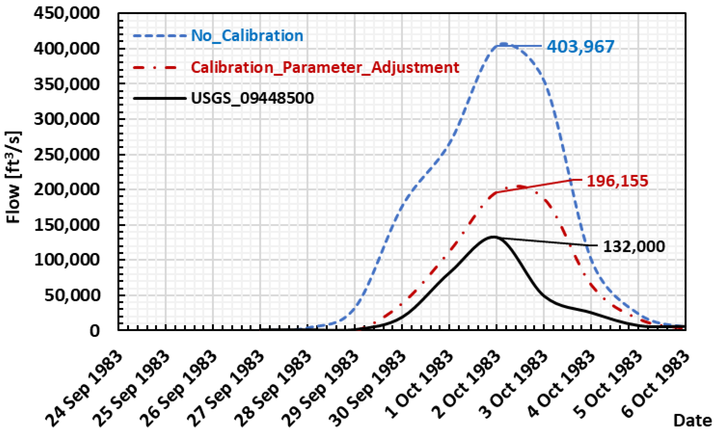
For preliminary outcomes, for regions with no HSG data, group D was conservatively chosen because it yielded minimal infiltration and consequently higher runoff potentials. The initial CN estimates were then incorporated into a hydrologic model where the peak discharge was estimated at the watershed outlet (identified by stream gage location on Figure 3). Applying the historical 1983 storm event (7-day, 27 September to 2 October of 1983), the model indicated a maximum daily peak discharge of 403,967 ft3/s at the outlet location on the Gila River (average daily peak discharge of 326,584 ft3/s). However, the USGS 09448500 stream gage at the same location recorded a peak flow of 132,000 ft3/s for this event (2 October 1983, Figure 4). It should be noted that the model result was inherently conservative since no impoundment or storage was considered upstream of the gage location, as a simplifying assumption.
The difference between the estimated peak discharge and USGS recorded peak flow highlights the necessity for model calibration through updating the input parameters, specifically the overly conservative assumption of HSG-D for regions with no HSG data. Through an iterative process performed on regions with no HSG data, it was discerned that CN corresponding to HSG-A resulted in a maximum daily peak discharge of 196,155 ft3/s (average daily peak discharge of about 163,825 ft3/s), which was about 50% higher than the USGS gage reading but considered reasonable as no upstream impoundment was incorporated in the model (Figure 4). Moreover, as can be seen in Figure 3, the CN results for the case study watershed are presented. The curve number is color-coded, with lighter shades of green representing lower CN values, indicating greater infiltration and lower runoff potentials, while darker green suggests the opposite. The sub-basin boundaries are highlighted in purple, and the state boundaries of New Mexico and Arizona are identified by a vertical, solid orange line. The map also features the USGS stream gage location and a few major dams located within this region.
5. Limitations and Future Improvements
Despite the robustness of the ArcMap tool developed in this study, there are inherent limitations that should be considered, especially those relevant to input information. The NLCD information usually comes in a large raster file. It is therefore suggested that the land cover raster data be clipped to a smaller area first (e.g., the state of Arizona rather than the entire United States) and then called within the tool.
In cases of dual representation of HSG, such as C/D, and in the absence of a user-defined CN table, the tool takes the value assigned to each HSG and takes the average as a preliminary estimate. For locations where soil data are not available to clearly define HSG, the tool utilizes values corresponding to HSG D. The future update of the tool is envisioned to adopt spatial averaging to fill in the missing or no data cells. It should be noted that there are different perspectives held on what would be an appropriate assumption for the mixed HSG curve number assumption [12].
Future improvements for the tool could focus on enhancing the flexibility of the CN and n table structures, allowing for easier customization and adaptation to specific project requirements. Additionally, there is potential to expand the tool’s functionality to support international projects, enabling the integration of multiple international data sources and coordinate systems. Another avenue for improvement could be the development of a mechanism to generate CN values based on soil saturation conditions, improving the details of the analysis. These improvements will further enhance the tool’s applicability and usefulness in various contexts.
6. Conclusions
In this paper, we introduce a unique ArcMap Python-based tool that simplifies and automates the computational process of key parameters in hydrologic analysis and hydraulic modeling, i.e., the SCS-CN and Manning’s n roughness coefficients, using the geospatial land cover data. Conceived in response to the growing need for geospatial input data for grid-based simulations in hydrology and hydraulic disciplines, the current tool efficiently fills the gap in the existing geospatial software toolbox collections.
Our innovative tool utilizes a user-specified watershed boundary to initiate the process of developing CN and Manning’s n geospatial layer. The tool calls the NLCD land cover and gSSURGO soil geodatabases to assign appropriate CN and Manning’s n to each land cover class within the watershed boundary defined by the user. The tool’s Python code can be modified to read lookup tables of interest or return outputs in a desired format by users with advanced knowledge of Python programming.
Further emphasizing its utility, our case study spanning a watershed across Arizona and New Mexico showcased the tool’s adaptability and its pivotal role in iterative refinement, particularly during the model calibration process. The discrepancies observed between model outputs and recorded data underscored the tool’s unique capability to allow user-driven adjustments, enhancing its potential in real-world applications. Additionally, this case study served as a testament to the tool’s functionality with extensive datasets, highlighting its robustness and relevance in contemporary hydrologic and hydraulic analyses.
Despite limitations related to the required structure of input data and the computational cost of large NLCD raster files, future enhancements are envisioned to incorporate more versatile features with less expected user inputs. The authors believe that the current tool makes a substantial contribution to streamlining and simplifying the computational process of key parameters in the field of hydrologic and hydraulic modeling while maintaining precision and flexibility. The tool can serve as an asset for engineers engaged in hydrologic analysis, hydraulic modeling, water resources planning and management, flood analysis and risk assessment, and environmental impact studies.
Author Contributions
For this research article, the following individual contributions were made: Conceptualization, B.A. and R.B.; methodology, B.A. and R.B.; software, B.A.; validation, B.A. and R.B.; formal analysis, B.A. and R.B.; investigation, B.A. and R.B.; resources, B.A. and R.B.; data curation, B.A. and R.B.; writing—original draft preparation, B.A.; writing—review and editing, R.B.; visualization, B.A.; supervision, R.B. All authors have read and agreed to the published version of the manuscript.
Funding
This research received no external funding.
Data Availability Statement
The data and tools used in this research are not publicly available but can be shared upon reasonable request.
Acknowledgments
The authors extend sincere appreciation to Joseph Rungee at Stantec for the initial version of the source code, upon which the current tool has been developed and refined. The authors invite users, clients, and future collaborators to share their insights or propose additional data sources that could enrich the toolbox’s capabilities. Such contributions are invaluable in advancing the toolbox’s performance. Please direct suggestions or proposed contributions to [email protected] and [email protected]. For the latest version of the toolbox, you can visit the tool GitHub page at “https://github.com/hydrology-hydraulics-innovations/CurveNumber.git” (accessed on 10 July 2023), where a training video was also uploaded for further clarification on how the tool can be utilized (access will be granted upon an email request sent to [email protected]).
Conflicts of Interest
The authors declare no conflict of interest.
References
- Ponce, V.M.; Hawkins, R.H. Runoff curve number: Has it reached maturity? J. Hydrol. Eng. 1996, 1, 11–19. [Google Scholar] [CrossRef]
- Chow, V.T. Open Channel Hydraulics; McGraw-Hill: New York, NY, USA, 1959. [Google Scholar]
- NRCS. National Engineering Handbook: Part 630—Hydrology; USDA Soil Conservation Service: Washington, DC, USA, 2004.
- Wickham, J.D.; Stehman, S.V.; Gass, L.; Dewitz, J.; Fry, J.A.; Wade, T.G. Accuracy assessment of NLCD 2006 land cover and impervious surface. Remote Sens. Environ. 2013, 130, 294–304. [Google Scholar] [CrossRef]
- Garen, D.C.; Moore, D.S. Curve number hydrology in water quality modeling: Uses, abuses, and future directions. JAWRA J. Am. Water Resour. Assoc. 2005, 41, 377–388. [Google Scholar] [CrossRef]
- Tillman, F.D. Documentation of Input Datasets for the Soil-Water Balance Groundwater Recharge Model of the Upper Colorado River Basin; No. 2015-1160; US Geological Survey: Reston, VA, USA, 2015.
- Arcement, G.J.; Schneider, V.R. Guide for Selecting Manning’s Roughness Coefficients for Natural Channels and Flood Plains; US Government Printing Office: Washington, DC, USA, 1989; Volume 2339.
- Järvelä, J. Determination of flow resistance caused by non-submerged woody vegetation. Int. J. River Basin Manag. 2004, 2, 61–70. [Google Scholar] [CrossRef]
- Zhan, X.; Huang, M.-L. ArcCN-Runoff: An ArcGIS tool for generating curve number and runoff maps. Environ. Model. Softw. 2004, 19, 875–879. [Google Scholar] [CrossRef]
- Janssen, C. Manning’s n Values for Various Land Covers to Use for Dam Breach Analyses by NRCS in Kansas; Revised by PAC; 2016. Available online: https://rashms.com/wp-content/uploads/2021/01/Mannings-n-values-NLCD-NRCS.pdf (accessed on 10 July 2023).
- Hydrologic Engineering Center. HEC-RAS 2D User’s Manual; USACE H. US Army Corps of Engineers: Davis, CA, USA, 2021. [Google Scholar]
- Hawkins, R.H.; Ward, T.J.; Woodward, D.E.; Van Mullem, J.A. (Eds.) Curve Number Hydrology: State of the Practice; American Society of Civil Engineers: Reston, VA, USA, 2008. [Google Scholar]
Figure 1.
Flowchart representing the steps of the tool.

Figure 2.
Screenshot of the Tool Interface and the Guidance Notes.

Figure 3.
CN Map for a Selected Watershed.

Figure 4.
Graphical representation of model estimated discharge vs. observed peak discharge at gage location. Note: The USGS streamflow daily records were scaled by the annual maximum flow record that occurred on 2 October 1983. To compare with observed flows, the daily maximum flow out of hourly simulated flows was considered.


Table 1.
Built-in Lookup Table of Land Cover and Hydrologic Soil Group-based Curve Number. SOURCE: [6].
Table 1.
Built-in Lookup Table of Land Cover and Hydrologic Soil Group-based Curve Number. SOURCE: [6].
| Land Cover Grid Code | NLCD Land Cover Description | Hydrologic Soil Group | |||
|---|---|---|---|---|---|
| A | B | C | D | ||
| 11 | Open Water | 100 | 100 | 100 | 100 |
| 12 | Perennial ice/snow | 40 | 40 | 40 | 40 |
| 21 | Developed Open Space | 49 | 69 | 79 | 84 |
| 22 | Developed Low Intensity | 77 | 86 | 91 | 94 |
| 23 | Developed Medium Intensity | 89 | 92 | 94 | 95 |
| 24 | Developed High Intensity | 98 | 98 | 98 | 98 |
| 31 | Barren Land | 77 | 86 | 91 | 94 |
| 41 | Deciduous Forest | 32 | 48 | 57 | 63 |
| 42 | Evergreen Forest | 39 | 58 | 73 | 80 |
| 43 | Mixed Forest | 46 | 60 | 68 | 74 |
| 52 | Shrub Scrub | 49 | 68 | 79 | 84 |
| 71 | Herbaceous | 64 | 71 | 81 | 89 |
| 81 | Hay Pasture | 49 | 69 | 79 | 84 |
| 82 | Cultivated Crops | 71 | 80 | 87 | 90 |
| 90 | Woody Wetlands | 88 | 89 | 90 | 91 |
| 95 | Emergent Herbaceous Wetlands | 89 | 90 | 91 | 92 |
Table 2.
Reasonable Range for Manning’s n Values Corresponding to Land Cover Classes and the Suggested Normal Value. Source: [10].
Table 2.
Reasonable Range for Manning’s n Values Corresponding to Land Cover Classes and the Suggested Normal Value. Source: [10].
| NLCD Land Cover Description | Allowable Range of n Values | Normal n Value for 2D Analyses (NRCS 2016) |
|---|---|---|
| Open Water | 0.025–0.050 | 0.040 |
| Developed, Open Space | 0.030–0.050 | 0.040 |
| Developed, Low Intensity | 0.080–0.120 | 0.100 |
| Developed, Medium Intensity | 0.060–0.140 | 0.080 |
| Developed, High Intensity | 0.120–0.200 | 0.150 |
| Barren Land | 0.023–0.300 | 0.025 |
| Deciduous Forest | 0.100–0.160 | 0.160 |
| Evergreen Forest | 0.100–0.160 | 0.160 |
| Mixed Forest | 0.100–0.160 | 0.160 |
| Scrub/Shrub | 0.070–0.160 | 0.100 |
| Grassland/Herbaceous | 0.025–0.050 | 0.035 |
| Pasture/Hay | 0.025–0.050 | 0.030 |
| Cultivated Crops | 0.025–0.050 | 0.035 |
| Woody Wetlands | 0.045–0.150 | 0.120 |
| Emergent Herbaceous Wetland | 0.050–0.085 | 0.070 |
Table 3.
Range Suggested for Infiltration or Loss Rates Corresponding to the SCS Hydrologic Soil Group Definition. Source: [11].
Table 3.
Range Suggested for Infiltration or Loss Rates Corresponding to the SCS Hydrologic Soil Group Definition. Source: [11].
| Hydrologic Soil Group | Range of Loss Rates (in/hr) (SCS 1986) |
|---|---|
| A—deep sand, deep loess, aggregated silt | 0.30–0.45 |
| B—shallow loess, sandy lam | 0.15–0.30 |
| C—clay loams, shallow sandy loam, soils low in organic content, and soils usually high in clay | 0.05–0.15 |
| D—Soils that swell significantly when wet, heavy plastic clays, and certain saline soils | 0.00–0.05 |
Disclaimer/Publisher’s Note: The statements, opinions and data contained in all publications are solely those of the individual author(s) and contributor(s) and not of MDPI and/or the editor(s). MDPI and/or the editor(s) disclaim responsibility for any injury to people or property resulting from any ideas, methods, instructions or products referred to in the content. |
© 2023 by the authors. Licensee MDPI, Basel, Switzerland. This article is an open access article distributed under the terms and conditions of the Creative Commons Attribution (CC BY) license (https://creativecommons.org/licenses/by/4.0/).
Share and Cite
MDPI and ACS Style
Alizadeh, B.; Berton, R. CN-N: A Python-based ArcGIS Tool for Generating SCS Curve Number and Manning’s Roughness. Water 2023, 15, 3581. https://0-doi-org.brum.beds.ac.uk/10.3390/w15203581
AMA Style
Alizadeh B, Berton R. CN-N: A Python-based ArcGIS Tool for Generating SCS Curve Number and Manning’s Roughness. Water. 2023; 15(20):3581. https://0-doi-org.brum.beds.ac.uk/10.3390/w15203581
Chicago/Turabian StyleAlizadeh, Babak, and Rouzbeh Berton. 2023. "CN-N: A Python-based ArcGIS Tool for Generating SCS Curve Number and Manning’s Roughness" Water 15, no. 20: 3581. https://0-doi-org.brum.beds.ac.uk/10.3390/w15203581
Note that from the first issue of 2016, this journal uses article numbers instead of page numbers. See further details here.