
Spatial Pattern and Driving Mechanism of Urban–Rural Income Gap in Gansu Province of China


1
College of Civil Engineering and Architecture, Jiaxing University, Jiaxing 314001, China
2
College of Architecture and Urban Planning, Lanzhou Jiaotong University, Lanzhou 730070, China
3
College of Landscape and Architectural Engineering, Guangxi Agricultural Vocational University, Nanning 530007, China
4
College of Urban and Environmental Science, Northwest University, Xi’an 710127, China
5
School of Architecture, Southeast University, Nanjing 210096, China
*
Author to whom correspondence should be addressed.
Land 2021, 10(10), 1002; https://0-doi-org.brum.beds.ac.uk/10.3390/land10101002
Submission received: 1 September 2021
/
Revised: 17 September 2021
/
Accepted: 20 September 2021
/
Published: 23 September 2021
(This article belongs to the Special Issue Urban-Rural-Partnerships: Sustainable and Resilient)
Abstract
:The urban–rural income gap is a principal indicator for evaluating the sustainable development of a region, and even the comprehensive strength of a country. The study of the urban–rural income gap and its changing spatial patterns and influence factors is an important basis for the formulation of integrated urban–rural development planning. In this paper, we conduct an empirical study on 84 county-level cities in Gansu Province by using various analysis tools, such as GIS, GeoDetector and Boston Consulting Group Matrix. The findings show that: (1) The urban–rural income gap in Gansu province is at a high level in spatial correlation and agglomeration, leading to the formation of a stepped and solidified spatial pattern. (2) Different factors vary greatly in influence, for example, per capita Gross Domestic Product, alleviating poverty policy and urbanization rate are the most prominent, followed by those such as floating population, added value of secondary industry and number of Internet users. (3) The driving mechanism becomes increasingly complex, with the factor interaction effect of residents’ income dominated by bifactor enhancement, and that of the urban–rural income gap dominated by non-linear enhancement. (4) The 84 county-level cities in Gansu Province are classified into four types of early warning zones, and differentiated policy suggestions are made in this paper.
1. Introduction
1.1. Background
Urban and rural areas are interrelated and interdependent, and together they contribute to the sustainable development of the regional economy. The urban–rural income gap is an important basis for measuring the capacity and level of comprehensive economic development of a country or region, as well as a crucial prerequisite for comprehensive and integrated urban–rural development. A large urban–rural income gap may then have a negative impact on economic and social development. Young [1] found that national income inequality is largely caused by the urban–rural income gap, accounting for about 40% of the total, according to an empirical analysis of 65 countries. The widening urban–rural income gap poses a great challenge to cities and villages in achieving sustainable development, and it has become an economic risk and social problem that developing countries have to face and solve in the process of industrialization and urbanization [2]. Therefore, it is of great theoretical significance and practical value to study the spatial patterns and influence factors of residents’ income and its changes and the urban–rural income gap and its changes, reveal their deep-seated driving mechanisms and further put forward targeted policy recommendations for narrowing the urban–rural income gap and achieving integrated urban–rural development.
As one of the countries with the largest urban–rural income gap in the world, China still has a large urban–rural income gap that is highly representative in the world. Therefore, the empirical study of China will provide inspiration or experience for other countries and regions in the world to solve the problems of residents’ income increase and urban–rural income gap. China has seen accelerated industrialization and urbanization as well as great achievements in economic growth and social development since its reform and opening up, bringing a dramatic increase in the income of urban and rural residents. However, the “miracle of development” is accompanied by a significant urban–rural income gap, which is increasing in a fluctuating manner. China’s urban–rural income ratio was about 2.51 in 1978, reached a historical peak of 3.33 in 2009, and remained at a high level of 2.64 in 2019, despite a decline. In the early 1990s, the income gap between urban and rural areas in China was less than $209, but in 2019 it widened to $3818. (The data comes from the China Statistical Yearbook in 1991 and 2020. According to the data released by the National Bureau of Statistics of China, the inflation rate in the same period is about 10%). As socialism with Chinese characteristics enters a new era, further narrowing the income gap between urban and rural areas has become an important part in solving the problem of “unbalanced development”. In the context of poverty eradication and high-quality development, comprehensive and integrated urban–rural development is facing more complex challenges, and the formulation of scientific policies to promote the reduction in the urban–rural income gap has become a hot issue of common concern among Chinese government sectors, scholars and the public. In recent years, both the central and local governments in China have included the urban–rural income gap as a core issue to be tackled in the 13th (2011–2015) and 14th (2016–2020) Five-Year Plans. In 2021, the central government issued the No. 1 document Opinions of the Central Committee of the Communist Party of China and the State Council on Comprehensively Promoting Rural Revitalization and Accelerating the Modernization of Agriculture and Rural Areas, clearly requiring “fully stimulating the development vitality of the countryside to consolidate and expand the results of poverty eradication and continue to narrow the income gap between urban and rural residents”.
1.2. Aim and Question
To sum up, the existing papers have provided abundant data for investigating the urban–rural income gap and lack a solid theoretical and methodological foundation for in-depth analysis of the spatial–temporal evolution law and driving mechanism of the urban–rural income gap. To address the shortcomings in the research on small cities, this paper attempts to take Gansu Province, a less developed region in western China, as an example, to systematically and quantitatively analyze the spatial and temporal patterns of the urban–rural income gap and its change patterns in 84 small county-level cities. Based on various measurement methods, such as GIS spatial analysis and the GeoDetector method, this paper tries to explore policy recommendations to promote integrated urban–rural development, so as to put forward a reference for Gansu and other similar regions in China and even the world, to coordinate urban–rural development and formulate plans or policies to narrow the urban–rural income gap.
This paper focuses on the following questions: (1) What are the regular characteristics of the spatial pattern and spatial effects of the urban–rural income gap in small cities, including the analysis and pattern identification of spatial heterogeneity and correlation characteristics of urban residents’ income, rural residents’ income and the urban–rural income gap? (2) What are the driving mechanisms of spatial variation in the urban–rural income gap in small cities, including the composition of influence factors, the size of direct effect and the interaction effect of multiple factors together? (3) How to create an early warning analysis model of urban–rural income gap in small cities and propose targeted response policies, including space governance risk classification and policy zoning?
2. Literature Review
The study of urban–rural income gap is a classical topic of geography, economics, sociology, planning and other subjects, and how to increase income and narrow the urban–rural income gap for residents is a hot issue of continuous concern for the government, scholars and the public. After a long-term follow-up study, academics have now achieved more fruitful research results in measurement methods, causes, coping strategies and social impacts, with continuous innovation of research fields and perspectives. For example, Attanasio [3] and Krueger [4] have extended the study of income inequality to the field of consumption inequality and analyzed the connection between the two. Additionally, Binelli [5], after an empirical study of Central and Eastern Europe, concluded that those with higher incomes are less aware of urban–rural income inequality. However, we find that there are still some shortcomings in the existing studies in research scale and methodology.
2.1. Review of Spatial Pattern
From the perspective of research scale, the research results are focused on the national and regional levels, with insufficient attention to the city scale, especially a great lack of empirical studies at the small city scale. At the national level, Burlacu [6], Tamkoc [7], Lise [8], Heshmati [9], Salvati [10], Thein [11], Bodjongo [12], Su [13] and other scholars have conducted case or empirical studies on the urban–rural income gap in Romania, Turkey, Japan, Korea, Greece, India, Myanmar, Cameroon and other countries, analyzing the gap changes. It is important to note that Zhao [14] and Gradin [15] conducted comparative analyses of China with the United States and China with India, finding that income inequality is much lower in China.
At the regional level, inter-provincial analysis is the focus. For example, Chen [16] pointed out that tourism, urbanization and fiscal decentralization all contribute to narrowing the urban–rural income gap in China. Shi [17] estimated the spillover effect of inbound tourism on the urban–rural income gap based on spatial econometric methods and concluded that inbound tourism significantly helps to reduce the income gap between urban and rural areas, but with striking differences between eastern, central and western regions. Kim [18] concluded that the interaction effect of tourism and (Foreign Direct Investment) in narrowing the urban–rural income gap is significantly larger in the autonomous regions than in other provinces, as the urban–rural income gap can be reduced through the use of FDI and the development of tourism in the autonomous regions. Li [19] found that the growth of Agricultural Environmental Total Factor Productivity further widened the urban–rural income gap in China. Jin [20] argued that the increase in social security spending helps reduce the urban–rural income gap, but there are significant regional differences in such effects. Wei [21] analyzed the effects of trade scale and mode on the urban–rural income gap at the provincial level in China and found that the scale of international import and export trade, processing trade and general trade has widened the urban–rural income gap in the eastern region, while having narrowed it in the central region. Meanwhile, in the western region, exports reduce while general trade aggravates the urban–rural income gap, but imports and processing trade have no significant effect. Hong [22] found a significant positive effect of upgrading China’s industrial structure on narrowing the urban–rural income gap, and Wang [23] concluded that the increase in urbanization level and fertilizer application intensity have a significant effect on alleviating the inter-provincial urban–rural income gap in China.
At the urban level, there have been some exploratory studies, but with insufficient attention to small and medium-sized cities and cities in less developed areas. For example, Zhang [24] conducted an empirical study on 248 prefecture-level cities from 2008 to 2018 and pointed out that tourism development helps to narrow the urban–rural income gap in China. Again, Huang [25] conducted an empirical study of 278 prefecture-level cities from 2003 to 2016, and the analysis showed that highway construction has reduced the urban–rural income gap, with great regional differences in its impact—negative in western cities while positive in eastern cities. Although Thiede [26] analyzed the dynamics of urban–rural income disparity in U.S. cities and concluded that the disparity in small cities is higher than that in large cities, there is a lack of analysis of the current characteristics, changing trends and main causes of urban–rural disparity in small cities. Small and medium-sized cities account for a large proportion and hold an important position in the regional town system. In addition, large-medium-small and prefecture-county-town-level cities, impacted by the scale effect, are greatly different in spatial heterogeneity and its driving mechanisms. Insufficient studies on small and medium-sized cities at the county and town levels, especially those in less developed areas, pose certain challenges to the applicability and accuracy of existing research findings.
2.2. Review of Driving Factors
From the perspective of research methodology, existing studies are focused on econometric analysis, with weak spatial analysis. The research methods of the existing papers are dominated by time series models, panel data models, mathematical statistics, correlation analysis, regression models, Markov chains, clustering, causality tests and cointegration equations, with focus on the analysis of the current characteristics, changing trends, influence factors, countermeasures and suggestions of urban–rural income gap. For example, Kibriya [27] analyzed the dynamics and patterns of rural–urban income inequality in India based on the time series method. Oyekale [28] analyzed the determinants of rural–urban income disparity in Nigeria based on regression methods and concluded that the factors of paid work, non-farm enterprises, grants and formal letters have the greatest impact on the rural–urban income gap, with further suggestion that infrastructure development, birth control and increased access to formal education in rural areas should be accelerated in order to reduce rural–urban income inequality. Sehrawat [29], based on least squares, cointegration equation and Granger Causality test tools, analyzed that financial development and economic growth reduce poverty in South Asian countries, while urban–rural income inequality increases poverty. Borodkin [30] analyzed the wage gap between urban and rural residents in the process of industrialization in Russia based on econometric methods. Chotia [31] analyzed the connection between infrastructure development and urban–rural income inequality in Bureau of Research Information Control System countries based on least squares and cointegration tests. Vafaei [32] investigated the connection between urban–rural income inequality and health based on ecological analysis, correlation analysis and multiple linear regression, finding that population health status is a function of absolute income, but not of relative income. Sehrawat [33] investigated the impact of financial development and economic growth on urban–rural income inequality in South Asian Association For Regional Cooperation countries based on the Granger Causality analysis tool. There are significant differences in the urban–rural income gap and its changes in different cities, and such differences represent the spatial heterogeneity under the combined effect of economic, social, political and ecological factors in the region, and it is often hard to explain the impact of spatial heterogeneity on the urban–rural income gap and its changes based on the above analysis methods. Besides, the existing papers give too little care to the influence of geospatial effect, lacking practical explanatory power and presentation. Most of the papers have an insufficient application of GIS spatial analysis tools and lack the necessary quantitative empirical studies on the influence factors of spatial heterogeneity and correlation, leading to insufficient awareness of the spatial patterns, spatial relationships, spatial effects and spatial dynamic mechanisms of urban–rural income gap in different regions.
In addition, there is no comprehensive study of multiple dependent and independent variables in the existing research methods, and no sufficient attention to multiple independent variable interaction effects. Most of the current papers are empirical studies on a particular indicator that reflects or influences the urban–rural income gap, yet often it is impossible for a single indicator to accurately depict the actual level of the urban–rural income gap and the complexity of its driving mechanisms. For example, Li [34] concluded that the high-speed rail construction has effectively narrowed the urban–rural income gap in China, but the convergence effect on the urban–rural income gap in China is still weak. Wang [35] concluded that the urban-biased land development policy is the most powerful factor driving the urban–rural income gap in China. Su [36] confirmed the existence of a Financial Kuznets Curve in East China; that is, the urban–rural income gap increases and then decreases with financial development. Batabyal [37] argued that income gap affects urban–rural population distribution patterns and residential choices, and Amara [38] concluded that educational attainment and family size are the major factors affecting urban–rural income gap in Tunisia. Zhao [39] analyzed the dynamic relationship between income structure and urban–rural income gap and its driving mechanism, and the results showed that wage income is the most powerful factor widening the urban–rural income gap, followed by transfer income, with the property income at the weakest position. Zhu [40] conducted an empirical study in China and concluded that the urban–rural inequality tends to be more severe in regions that have more complex export product/destination structures, due to the concentration of export activities in urban areas and due to some barriers that inhibit the flow of input factors (e.g., capital and labor) between rural and urban areas. Chen [41] found that while FDI directly contributes to narrowing the urban–rural income gap through job creation, knowledge spillovers and contributions to economic growth, it also exacerbates urban–rural income inequality through international trade and other channels. The urban–rural income gap and its changes are influenced by many factors, and they are in a complex interaction relationship. The joint action of multiple factors may produce synergistic reinforcing effects or antagonistic constraining effects, which eventually lead to deformation or even denaturation of the driving force under the influence factors alone. However, the quantitative measurement and in-depth analysis are neglected in the existing papers. In the era of big data, comprehensive research based on multiple indicators as dependent and independent variables is imminent.
3. Research Design
3.1. Research Methods
3.1.1. Coefficient of Variation: CV
The coefficient of variation (CV) is used to compare the magnitude of dispersion of the analyzed data, which is independent of the magnitude and measurement scale. The coefficient of variation is dimensionless, and a larger value represents a greater degree of dispersion, and vice versa. According to Guan [42], Zhang [43], Ruan [44], Liu [45], Miyamoto [46] and She [47], dispersion is classified as weak, medium and strong based on the CV values. That is, the value of the coefficient of variation is weakly discrete when it is 0–0.15, reflecting the low spatial inequality of urban–rural income gap; moderately discrete when it is 0.16–0.35, reflecting the high spatial inequality of urban–rural income gap; and strongly discrete when it is greater than 0.36, reflecting the very high spatial inequality of urban–rural income gap.
The coefficient of variation is calculated according to the equation as follows:
where represents the coefficient of variation, n represents the number of small cities in the study area and represents the observed value of an indicator for the small city; is the average of the observed values of an indicator for all small cities. It is important to note that when the average value is close to zero, even a tiny perturbation may have a large impact on the coefficient of variation, resulting in poor accuracy. Therefore, when the average value is close to zero, the coefficient of variation values is only of reference value and cannot be used as a basis for determining spatial differentiation.
3.1.2. Exploratory Spatial Data Analysis: ESDA
ESDA is an ideal data-driven analysis method recognized by academic circles that has been widely used in the study of spatial heterogeneity and correlation. The commonly used measures in exploratory spatial data analysis methods are the global Moran’s I, the Moran’s scatter plot and the Lisa agglomerative distribution plot. In this paper, the global Moran index is employed to indicate the existence of spatial autocorrelation, agglomeration and agglomeration trend in the overall space, and further explain the agglomeration types and spatial correlation characteristics in existence in terms of spatial location through the Lisa agglomeration distribution map, reflecting the spatial heterogeneity and instability within the local area. The value of Global Moran’s I is in a range of [−1, 1]. At a given significance level (generally 0.05 or 0.1), the value > 0 indicates positive spatial correlation, and when the value is greater, the spatial correlation and agglomeration will be more significant; the value < 0 indicates negative spatial correlation, and when the value is smaller, the spatial variation will be larger; the value = 0 indicates random spatial distribution. According to Local Moran’s I, spatial correlation patterns can be subdivided into four types, including H-H and L-L with positive spatial correlation and H-L and L-H with negative spatial correlation. The calculation equation is as follows:
where n represents the quantity of cities, and are the observed values of cities and , respectively, is the average of the observed values, is the spatial weight matrix in global spatial autocorrelation and the row normalized value of spatial weights in local spatial autocorrelation, is the sum of spatial weight matrices, and are the normalized values of the observed values of cities and . In this paper, we have conducted spatial autocorrelation analysis based on ArcGis 10.2 (Esri, Redlands CA, USA) and GeoDa 1.18 (Esri, Redlands CA, USA), where the significance level is 0.05, the spatial weight matrix is the one based on the adjacent boundaries and all parameters are those of software by default. The maximum number of neighbors is 11 and the minimum is 1, with the average of 4.64 and the median of 4.50.
3.1.3. Boston Consulting Group Matrix: BCG
BCG, also known as the four-quadrant analysis, was created in 1970 by Bruce Henderson, a leading American management scientist and founder of the Boston Consulting Group. This method is mainly applied in business management and economics, and it classifies products or markets into four types: stars, question, cows and dogs, through the interaction of two factors of “sales growth” and “market share”. In this paper we use it to evaluate the spatial classification of residents’ income and the risk partitioning of urban–rural income gap, depending on the average of the relative shares of the dependent variables and growth rates to classify the cities in the study area into four types of H-H, H-L, L-H, and L-L.
where t represents the time, and are the observed value of city and the maximum value of all cities, respectively, and is the observed value of city i in the base period.
3.1.4. GeoDetector
GeoDetector is a new spatial analysis model used to detect the connection between a certain geographical attribute and its explanatory factors [48] and is widely used in the study of the influence factors of natural and economic and social phenomena. This paper is devoted to exploring the spatial pattern of urban–rural income gap in small cities and the driving forces behind it, and this method is quite applicable to it due to a large number of influence factors. It should be noted that an exploratory study has been conducted in this regard by Chen [49], who empirically investigated the spatio-temporal characteristics of the urban–rural income gap and its drivers in prefecture-level cities in the Yangtze River Economic Belt from 2000 to 2017. GeoDetector consists of four functional modules of factor detection, interaction detection, risk detection and ecological detection. In this paper, we studied the magnitude of factor forces and its interaction effects that affect the spatial pattern of urban–rural income gap in county-level cities in Gansu depending on the two functional modules of factor detection and interaction detection.
Spatial differentiation is the spatial expression of natural and socio-economic processes. GeoDetector is a new statistical method to detect spatial heterogeneity and reveal its driving factors. Its basic idea is that, based on the assumption that the study area is divided into sub-regions, there is spatial heterogeneity if the sum of the variances of the sub-regions is smaller than the total regional variance, and there is statistical correlation between the independent and dependent variables if their spatial distribution tends to be the same. In other words, if independent variables have a significant influence on dependent variables, they should have similar spatial distributions [50]. The q-statistic calculated by GeoDetector can be used to measure the degree of explanation of independent variables to dependent variables and analyze the interaction between independent variables. In factor detection, GeoDetector, by calculating the q-value of each independent variable and dependent variable, quantitatively evaluates the correlation (similarity) between the two. In interaction detection, GeoDetector determines whether there is interaction between two independent variable factors, and the strength, direction, linearity or nonlinearity of interaction by calculating and comparing the q-value of the dependent variable after superposition of two independent variable factors.
Let’s assume the dependent variable is and the independent variable is , and use them to depict the level of urban–rural income gap and its influence factors, respectively. With the value of the factor detection results, the level of spatial heterogeneity of and the extent to which explains the spatial heterogeneity of can be measured. The value of is in a range of [0, 1], and under the condition of passing the significance test, a larger value indicates that has a more pronounced spatial heterogeneity and has a stronger explanatory power for it. In general, the threshold value for passing the significance test is 0.05 under general conditions, and 0.1 under loose conditions. With the interaction detection results we can identify interactions between different drivers , i.e., to assess whether drivers and , when acting together, enhance or diminish the explanatory power of the dependent variable , or whether the effects of these factors on are independent of each other. The evaluation results are classified into five categories according to the relationship between and , under the interaction of the two drivers (Table 1) [51]. The calculation equation of q is as follows:
where h is the number of strata or classifications of the independent variables, and N are the number of cities in stratum h and the study area, respectively, and are the variance of the dependent variable in stratum h and the study area, respectively, SSW is the Within Sum of Squares and SST is the Total Sum of Squares.
3.2. Study Area: Gansu
The study area of this paper is 84 county-level small cities in Gansu Province, and due to a great lack of data for Anning, Jiashishan and Maqu, they are not included in this study to ensure the accuracy of the findings (Figure 1). Located in the hinterland of northwest China, Gansu Province is one of the major minority populated areas in China, and it is a typical underdeveloped province in China with backward economic and social development. In 2019, the GDP of Gansu Province was 126.4 billion US dollars, ranking fifth from the bottom among 31 provinces, autonomous regions and municipalities directly under the central government of China; during the same period, its per capita GDP was $4783, ranking first from the bottom in the country (Figure 2). At present, the problems of inadequate rural development, unbalanced development between urban and rural areas, and especially the large income gap between urban and rural areas, are still prominent in Gansu Province. In 2019, the average income of urban residents in Gansu Province was $4685.51, $1454.66 lower than the Chinese average; the average income of rural residents was $1395.80, $926.58 lower than the Chinese average; the absolute difference between urban and rural income reached up to $3289.85, $528.23 lower than the Chinese average; and the urban–rural income gap index reached 3.36, 0.7 higher than the Chinese average (Figure 3).
From the perspective of the development of Gansu Province, although the average income of rural residents in Gansu Province has been growing faster than that of urban and rural areas in recent years, and the urban–rural income gap has been gradually narrowing, the absolute gap between urban and rural incomes is still in a rapid and sustained growth, with the gap still stable at a high level and greater than the national average all the time (Figure 4). From 2013 to 2019, the average income of urban residents in Gansu Province increased by $1805, up by 7.20% annually; the average income of rural residents increased by $586, up by 8.08% annually; the absolute urban–rural income gap increased by $1219, up by 6.84% annually; the urban–rural income gap index decreased by 0.20, up by −0.82% annually. In summary, the income level of residents in Gansu province is much lower than the average of China, but its urban–rural income gap index is much higher than the national average level. It is a major task for governments at all levels in Gansu Province to increase residents’ income and narrow the urban–rural income gap for a long period of time in the future. The study on Gansu province is a typical case, and it is of great reference value for other similar regions in China and the world, to solve the problems of income increase and urban–rural income gap.
3.3. Index Selection
From the perspective of dependent variable selection, the average incomes of urban residents and that of rural residents are the basic indicators, serving as the most intuitive ones for studying the urban–rural income gap and significant ones for the government to examine the coordination of regional urban–rural economic and social development. The ratio of the two can be used to construct the index of urban–rural income gap. It should be noted that narrowing the urban–rural income gap is the core of policy design, and for the government and the public, in addition to the status quo values of the three indicators above, they are also interested in the changes of these indicators. Therefore, in this paper, we finally selected six dependent variables, that is, the average income of urban residents, the average income of rural residents, the urban–rural income gap index, the change in the average income of urban residents, the change in the average income of rural residents and the change in the urban–rural income gap index (Table 2). There are many factors influencing the urban–rural income gap, and they are in a complex relationship. The analysis in part 1.2 shows that existing studies focus on urban-biased policies, a dualistic economic system, urbanization, industrialization, economic outward orientation, financial development, institutional change, natural conditions, education level and agricultural inputs [52], which are of great inspirational values for this study. The urban–rural income gap and its changes constitute a systematic problem. In line with the principles of comparability, feasibility, representativeness and accessibility, and according to the research ideas of Li [53], Zhao [54,55] and Yuan [56], this paper presents a comprehensive analysis of their influence factors based on 13 indicators from three areas of economy, society and policy (Table 2).
The impact of the economic development level on the urban–rural income gap is shown in the total amount and quality, and it is also in a greater connection with the industrial structure and consumption level [57]. GDP and per capita GDP are common indicators to depict the total amount and quality of urban economic development, while retail sales of social consumer goods are commonly used indicators to reflect consumption vitality. The value added by the secondary and tertiary industries is a major driver to attract population and increase income, presenting the degree of deagrarianization of the industrial structure and its employment and wealth creation effects. The key to the impact of social conditions on the urban–rural income gap lies in population size and its attribute characteristics. Population size, population mobility and the transformation of rural population to urban population have a great influence on the urban–rural income gap by differentially improving the marginal efficiency between rural and urban areas. We should note that the Internet and its applications have enjoyed a strong rise in China and have been integrated into all areas of the social economy, leading to the rapid growth of new businesses such as e-commerce live streaming and short video, as well as the size of online shopping users. The Internet has played a role as a “booster” in increasing farmers’ income, selling agricultural products and transforming agriculture. As an emerging force, the Internet has reduced the cost of information search and opened up the scope of market participation for farmers, and has improved the accuracy of government policies for agricultural benefits. The popularization and development of the Internet has brought a powerful digital dividend for the development of rural areas, farmers and agriculture, and has become a major emerging factor that should not be ignored in the study of the urban–rural income gap in China in the new era.
Government initiative is the key to solving the problem of the urban–rural income gap. With direct fiscal spending, indirect bank loans and comprehensive policy design, the government can effectively macro-regulate the income of urban and rural residents. Local governments with greater fiscal strength have a greater ability to intervene directly, so we selected in this paper the size of fiscal spending to represent direct government influence. The low profitability of the agriculture-related industries makes it difficult to get loans from banks in general. For this reason, the government often indirectly intervenes in the urban–rural income gap by establishing agricultural policy banks and increasing the targeted loans related to agriculture to guide bank loans to rural areas, agriculture and farmers. The main functional area planning is a long-term strategic program in China, and it divides the space into different types of policy areas based on the resource and environmental carrying capacity, existing development density and development potential of different regions. As the main functional area planning directly determines the main function, development direction and intensity of each city, it has been a major policy that has to be considered in the study of the urban–rural income gap. In November 2015, the central government issued the Decision on Winning the Battle against Poverty, marking that poverty alleviation has become a core task for the central and local governments. In 2016, there were 592 national-level, poverty-stricken counties in China, including 375 in the western region. Gansu had a total of 75 poverty-stricken counties, including 58 at the national level and 17 at the provincial level, making it one of the provinces with the heaviest task of poverty eradication in China. Since the implementation of the war on poverty, the state has increased investment and policy support for Gansu Province, especially for poverty-stricken counties, all of which have now lifted themselves from poverty. In the transformation of Gansu province from a concentration of poor counties to a region with no poor counties, it can be seen that the impact of poverty alleviation policy on the urban–rural income gap in the province is obvious.
3.4. Research Steps
This study consists of three steps and seven key points (Figure 5). The first step is raw data and pre-processing. (1) Form a complete raw data table based on the data published on the relevant statistical websites. (2) Discrete the continuous data of independent variables based on Python and, to eliminate artificial influence, classify the independent variables of 84 county-level cities into nine types by the percentile method (2–10). The second step is data processing. (3) Perform a spatial analysis, including the calculation of the coefficient of variation of the dependent variable and Moran’s I, and spatial analysis of the dependent variable based on ArcGis 10.2 and GeoDa1.18. (4) For Influence Factor, import the original data of the dependent variable and the discrete data of the independent variable into GeoDetector, carry out factor detection and interaction detection, and perform data review and result selection according to p-value (<0.05, <0.1 under loose conditions) and q-value. The third step is data analysis. (5) Comprehensively analyze the forces of driving factors and their acting modes, grade and classify the factors and their interaction effects. (6) Spatially classify the income level of residents, spatially classify the income gap and make adaptive and targeted policy recommendations based on the BCG model.
3.5. Data Sources
The dependent and independent variable indicators in this paper are mainly from the Gansu Development Statistical Yearbook and the Gansu Province Rural Yearbook, and some indicators are from the China County Construction Statistical Yearbook, with some missing data collected from the statistical handbooks and government work reports of each county. The study period chosen was 2016–2019, for two main reasons. The first is to ensure data integrity. There were indeed many statistics before 2016, and lengthening the study time would affect the accuracy of the conclusions. The second is to maintain the consistency of the policy context. In November 2015, China started the battle against poverty, with the central and provincial governments strengthening support for poverty-stricken counties and impoverished people. Due to the high proportion of county-level cities in Gansu Province defined as poverty-stricken counties by the central and provincial governments, and the large impact of poverty eradication and poverty alleviation policies, the analysis of 2016 as the base year is more reasonable considering the lag in policy implementation. It should be noted that the main functional area planning divides the space into three types of ecological areas, main agricultural products production areas and key development areas, so they are assigned values of 1, 2 and 3 respectively in the processing of independent variables. In addition, the poverty-stricken counties involve both national and provincial levels, so the 84 counties in Gansu Province are classified into three types: general counties, provincial poverty-stricken counties and national poverty-stricken counties, and they are assigned values of 1, 2 and 3, respectively, in the processing of independent variables.
4. Results
4.1. Spatial Pattern
4.1.1. Spatial Heterogeneity
There is some spatial heterogeneity in residents’ income and its changes and in urban–rural income gap and its changes in 84 county-level cities in Gansu Province, but it is not very prominent. The spatial heterogeneity of rural residents’ income and its changes is at the highest level, followed by the spatial heterogeneity of urban residents’ income and its changes, with the spatial heterogeneity of urban–rural income gap and its changes at the bottom. In 2019, the coefficients of variation for , and were 0.19, 0.25 and 0.24, respectively, in a range of 0.16~0.35, which were moderately heterogeneous; the coefficients of variation for and were 0.44 and 0.41, respectively, both greater than 0.36, which were strongly heterogeneous. showed a large number of negative numbers, with an average value of −0.08 and a standard deviation of 0.12, indicating a low level of spatial heterogeneity. In 2016, the coefficients of variation for and were 0.20 and 0.26, respectively, which remained moderately heterogeneous, and the coefficient of variation for was 0.51, which was strongly heterogeneous. The indicators related to urban–rural income gap of 84 county-level cities in Gansu Province in 2019 and 2016 were classified into high, medium and low types by nature breaks of ARCGIS 10.2.
In terms of the spatial distribution of state quantities, and have similar spatial patterns, and is completely different from the first two. Besides, the spatial pattern in 2019 was generally similar to that in 2016, except for a broad contraction in the medium category of , indicating the appearance of a solidified spatial pattern of the urban–rural income gap (Figure 6). In 2019, and shared the same spatial pattern, with the exception of the area around the provincial capital, the three types of cities were characterized by southeast-northwest clustering and stair-step distribution. Specifically: cities of the high type are mostly distributed in the northwest corner of Gansu, including Guazhou, Jinta, Subei, Dunhuang, Sunan and Jinchang, with a small proportion in the core area of the provincial capital, including Chengguan, Anning and Xigu. Cities of the medium type are concentrated in the west corridor of the Yellow River and the edge of the provincial capital, including Shandan, Minle, Ganzhou, Yongchang, Minqin, Yongdeng, Gaolan and Yuzhong. Cities of the low type are concentrated in the eastern region of the Yellow River, including Linxia, Longxi, Huining, Xihe and Liangdang. is completely different from and , with high agglomeration but insignificant stepwise. Cities of the high type are mainly distributed in the west region of the Yellow River, including Xihe, Zhouqu, Longxi and Huachi, with a small proportion in the west corridor of the Yellow River, including Gulang and Tianzhu. Most of the medium type cities are concentrated in the edge of the provincial capital, including Jingtai, Baiyin, Jingyuan, Huining, Yongjing and Linxia, with a small proportion scattered in the east region of the Yellow River, including Zhengning, Lingtai, Huixian and Chengxian. Cities of the low type are mainly distributed in the west corridor of the Yellow River and the provincial capital area, including Guazhou, Yumen, Sunan, Minqin, Yongdeng, Gaolan, Chengguan and Xigu. In 2010, changed significantly, and the number of the medium type cities increased rapidly, with the geographical scope expanding from the west region of the Yellow River to the east. Unfortunately, and remain unchanged, and the spatial pattern is solidified.
From the perspective of the spatial distribution of changes, the spatial patterns of , and are completely different (Figure 7). For , cities of the high type are mainly distributed in regions of Lanzhou and Jiuquan, including Yongdeng, Gaolan, Chengguan, Yuzhong, Yumen, Subei, Xifeng and Jinchuan. There are agglomerations of the medium-type cities in both the west and east regions of the Yellow River, the former including desert oasis cities such as Jinta, Guazhou, Dunhuang, Sunan, Yongchang and Minle, and the latter including resource-based cities such as Huachi, Heshui, Zhengning, Zhenyuan, Lingtai, Chongxin and Jingchuan. Cities of the low type are mainly distributed in the east region of the Yellow River, including Liangdang, Diebu, Longxi, Wushan, Kangle, Xiahe, Jingyuan and Jingtai, with a small proportion in the west corridor of the Yellow River, including Minqin, Gulang, Tianzhu, Gaotai and Linze. For , cities of the high type are mainly distributed in the northwest of Gansu Province, including Subei, Yumen, Jinta, Sunan and Jinchuan. Cities of the medium type are mainly distributed in the west corridor of the Yellow River and the Lanbai metropolitan area, including Guazhou, Dunhuang, Minqin, Shandan, Ganzhou, Minle, Baiyin, Gaolan and Yongdeng. All of the low-type cities are located in the east region of the Yellow River, including Qin’an, Tongwei, Weiyuan, Longxi, Gangu and Dongxiang. For , cities of the high type are all concentrated in the provincial capital metropolitan area, including Yongdeng, Chengguan, Yuzhong and Gaolan. All the cities in the west corridor of the Yellow River and the cities in the area with intensive mineral resources in the east region of the Yellow River are of the medium type, including Heshui, Jingning, Zhengning, Huating and Lingtai. It should be noted that the spatial patterns of income growth for urban and rural residents are quite different. For urban residents, the cities with the highest income growth rate are distributed in the core area of the provincial capital, while those with the lowest income growth rate are distributed in ethnic autonomous regions, with the income growth of the urban residents in cities along the Longhai Railway, highways and the Yellow River, as well as oasis cities in the west corridor of the Yellow River, and resource-based cities in the east region of the Yellow River at a medium rate. For rural residents, the cities with the highest income growth rate are distributed in the ethnic autonomous regions, and those with the lowest growth rate in the west corridor of the Yellow River, with the income growth in most of the cities in the east region of the Yellow River at a medium rate.
4.1.2. Spatial Correlation
The indicators related to the urban–rural income gap in 84 county-level cities in Gansu Province are all positively spatially autocorrelated, and they are ranked as > > > > > in spatial correlation strength. From the perspective of global Moran’s I, the value of in 2019 and 2016 was 0.34 and 0.26, respectively, always at a low level; the value of was 0.67 and 0.68; the value of was 0.66 and 0.68; and the values of , , and were 0.52, 0.60 and 0.43, respectively, always at the middle and high level, indicating that the urban–rural income gap and its changes in county-level cities in Gansu Province remain stable for a long time with significant global spatial autocorrelation and strong spatial agglomeration. To further analyze the types of spatial interconnections among cities, we created a Lisa diagram by means of GeoDa 1.18. Based on the spatial relationship between the sample cities and their neighboring cities, the cities were classified into four types of H-H, H-L, L-H, and L-L (Figure 8 and Figure 9). , and are roughly the same in spatial pattern in 2016 and 2019, with changes only in local areas, such as the L-L type of expanding widely in the Dingxi region, and the addition of Jingchuan and Huixian for the L-H type of besides Kongtong. and are similar in spatial pattern, with the latter developing at a higher level than the former. is obviously different from and . It should be noted that the spatial patterns of the amount and rate of change of urban–rural income and its gap also vary widely.
For , cities of the H-H type are concentrated in the northwest region of Gansu in a contiguous distribution, and those of the L-L type are mainly concentrated in Dingxi and Gannan regions, indicating that when the income of urban residents in the central county is high/low, that of the neighboring counties is high/low, characterized by a strong positive spatial correlation; the only cities of the L-H type (polarized) are Minqin and Gaolan, and no cities are of the H-L type (hollow), indicating that there are few cases where the income of residents in neighboring counties is low/high when that in the central county is high/low, with the negative spatial correlation quite insignificant. is very similar to , but the H-H and L-L types have a broader geographic coverage. It should be noted that has no L-H type, and only one city, Linxia, is of the H-L type. For , cities of the H-H type are concentrated in Longnan, Tianshui, Pingliang and Qingyang areas in the southeast of Gansu Province in a contiguous distribution; cities of the L-L type are mainly concentrated in the west of the Yellow River and the provincial capital area; cities of the L-H type are only Kongtong, Jingchuan and Huixian, and there is only one city, Tianzhu, of the H-L type. For and , cities of the H-H type are mainly concentrated in the northwest of Gansu Province, and cities of the L-L type are mainly located in the southwest corner of Gansu. It should be noted that has only one city of L-H and H-L types, Minqin and Qinzhou, respectively; has no cities of the L-H type, and there is only one city, Linxia, of the H-L type. For , cities of the H-H type are mainly distributed in the provincial capital and have expanded to the northwest to oasis cities such as Sunan and Tianzhu with minority autonomy, cities of the L-L type are also clustered in the southwest region of Gansu Province, Qinzhou and Linxia are cities of the H-L type and there is only one city, Jingtai, of the L-H type.
It is important to note that from the perspective of the spatial distribution of the rate of change, the patterns of urban residents’ income, rural residents’ income and urban–rural income gap are different from each other. As for the change rate of urban residents’ income, cities of the H-H type are concentrated in the southeast corner of the provincial capital, cities of the L-L type are concentrated in Linxia Hui Autonomous Prefecture and the Longnan region, Baiyin and Jingtai are cities of the L-H type, and there are no cities of the H-L type. For the rate of change of rural residents’ income, cities of the H-H type are concentrated in the Hedong Hui and Tibetan autonomous regions and Longnan region, cities of the L-L type are concentrated in the west corridor of the Yellow River, Hezuo and Qinzhou are cities of the L-H type and there are no cities of the H-L type. For the change rate of urban–rural income gap, there are few cities of the H-H type—only Qilihe, Xigu, Chengguan and Gaolan in the core area of the provincial capital. There are many cities of the L-L type, which are concentrated in the autonomous region for ethnic minorities in the east of the Yellow River. Baiyin and Jingtai are cities of the L-H type, and there is only one city, Qizhou, of the H-L type.
4.2. Influence Factors
4.2.1. Factor Detection
of and , , and of could not pass the significance test, while of and of could only pass the significance test of 0.1. At 5% or a more stringent level of significance, the impact factors are classified as high, medium and low based on the ranking of the direct effect (q) according to top3, top7 and others (Table 3). For the average income of urban residents, per capita GDP, alleviating poverty policy, and urbanization rate are of the high type; floating population, added value of secondary industry, GDP and number of Internet users are of the medium type; total retail sales of consumer goods, added value of tertiary industry, amount of bank loans, main functional area planning and financial expenditure are of the low type. The social driving force is greater than the economic driving force in general, and the policy driving force is minimal. For the average income of rural residents, per capita GDP, alleviating poverty policy and urbanization rate are of the high type; floating population, GDP, added value of secondary industry and added value of tertiary industry are of the medium type; number of Internet users, financial expenditure, amount of bank loans, total retail sales of consumer goods, main functional area planning and total population are of the low type. The social, economic and policy driving forces are roughly equal in general, and all of them are strong. For the urban–rural income gap index, per capita GDP, urbanization rate and alleviating poverty policy are of the high type; floating population, added value of secondary industry, financial expenditure and amount of bank loans are of the medium type; GDP, total retail sales of consumer goods, added value of tertiary industry, main functional area planning, total population and number of Internet users are of the low type. The social, economic and policy driving forces are roughly equal in general, and all of them are weak (Figure 10).
For changes in average income of urban residents, per capita GDP, added value of secondary industry and GDP are of the high type; urbanization rate, alleviating poverty policy, number of Internet users and amount of bank loans are of the medium type; total retail sales of consumer goods, added value of tertiary industry, floating population and main functional area planning are of the low type. The social and policy driving forces are roughly equal in general, lagging well behind the economic driving force (Figure 10). For changes in average income of rural residents, per capita GDP, alleviating poverty policy and urbanization rate are of the high type; floating population, added value of secondary industry, GDP and added value of tertiary industry are of the medium type; number of Internet users, amount of bank loans, total retail sales of consumer goods, financial expenditure and main functional area planning are of the low type. The social driving force is greater than the economic force in general, and the policy driving force is minimal (Figure 10). For changes in urban–rural income gap index, added value of secondary industry, per capita GDP and GDP are of the high type; total retail sales of consumer goods, amount of bank loans, added value of tertiary industry and number of Internet users are of the medium type; main functional area planning, alleviating poverty policy and urbanization rate are of the low type. The social and policy driving forces are roughly equal in general, lagging well behind the economic driving force (Figure 10).
4.2.2. Interaction Detection
All of the factor pairs are bifactor-enhanced or non-linearly enhanced with each other, and there are no independent and asymptotic relationships. The factor pairs can be classified into three types of high, medium and low based on the top10 and average value of the factor pair interaction forces (Figure 11).
forms a total of 66 factor pairs, and the average value of the interaction forces is 0.68, with the minimum value of 0.37 and the maximum value of 0.90; the interaction effects of ∩ and ∩ are greater than 0.90. The factor pairs are dominated by bifactor enhancement effects, and there are only 12 non-linearly enhanced factor pairs, accounting for about 18.18%, including ∩, ∩, ∩, ∩, ∩, ∩, ∩, ∩, ∩, ∩, and ∩. is the uppermost interaction factor.
forms a total of 78 factor pairs, and the average value of the interaction forces is 0.71, with the minimum value of 0.29 and the maximum value of 0.95; the interaction effects of ∩, ∩, ∩, ∩, ∩, and ∩ are greater than 0.90. The factor pairs are dominated by bifactor enhancement effects, and there are a significantly increasing number of non-linearly enhanced factor pairs, up to 27, accounting for about 35.90%, including ∩, ∩, ∩, and ∩. The uppermost interaction factors are , , , , and .
forms a total of 78 factor pairs, and the average value of the interaction forces is 0.51, with a minimum value of 0.12 and a maximum value of 0.83; the interaction effects of ∩, ∩, ∩ and ∩ are greater than 0.80. The non-linear enhanced factors dominate, up to 57, accounting for about 73.08%, including ∩, ∩, ∩, ∩, ∩, ∩, ∩, ∩ and ∩. All factors except have a significant interaction effect.
forms a total of 55 factor pairs, and the average value of the interaction forces is 0.69, with the minimum value of 0.48 and the maximum value of 0.92; the interaction effects of ∩ and ∩ are greater than 0.90. The factor pairs are dominated by bifactor enhancement effects, and there are only 12 non-linearly enhanced factor pairs, accounting for about 21.82%, including ∩, ∩, ∩, ∩, ∩, ∩, ∩, ∩, and ∩. The uppermost interaction factors are and .
forms a total of 66 factor pairs, and the average value of the interaction forces is 0.73, with the minimum value of 0.37 and the maximum value of 0.95; the interaction effects of ∩, ∩, ∩, ∩, ∩, ∩, ∩ and ∩ are greater than 0.90. The factor pairs are dominated by bifactor enhancement effects, and there are only 20 non-linearly enhanced factor pairs, accounting for about 30.30%, including ∩, ∩, ∩, ∩, ∩, ∩, ∩, ∩ and ∩. The uppermost interaction factors are , , and .
forms a total of 45 factor pairs, and the average value of the interaction forces is 0.54, with the minimum value of 0.13 and the maximum value of 0.93; only the interaction effect of ∩ is greater than 0.90. The factor pairs are dominated by non-linear enhancement effects, up to 13, accounting for about 73.33%, including ∩, ∩, ∩, ∩, ∩, ∩, ∩, ∩ and ∩. The uppermost interaction factors are , , and .
5. Discussion
5.1. Low Spatial Heterogeneity, High Spatial Correlation and Agglomeration, and Solidified Stepwise Spatial Pattern
The income of rural residents and its changes show strong spatial heterogeneity, but there is no high spatial heterogeneity of the income of rural residents and its changes or the urban–rural income gap index and its changes. However, the spatial correlation and agglomeration of the dependent variables of urban residents’ income is high, except for the relatively low spatial correlation. From the perspective of spatial pattern and its evolution trend, the 84 county-level cities in Gansu Province are in a very stable spatial pattern, prominently characterized by high, medium and low stepwise aggregated distribution. The spatial distribution and change patterns of , , and show that the residents in the Lanzhou-Baiyin metropolitan area and the Jiuquan-Jiayuguan co-location area are the most affluent, with the most significant income growth of urban and rural residents, followed by the residents in the west corridor of the Yellow River (Zhangye–Jinchang– Wuwei section) with a high income growth of urban and rural residents, and then the residents of the east region of the Yellow River have the smallest income growth of urban and rural residents. also follows the pattern of stepwise spatial distribution and change, and the urban–rural income gap is highly coupled with the poverty level, indicating that the income gap is greater in poorer places. has a completely different spatial pattern, with the largest changes in urban–rural income gap concentrated in the provincial capital area, moderate changes in oasis cities and resource-based cities and the smallest changes in non-resource-based cities in the west region of the Yellow River. It should be noted that the spatial patterns of the amount and rate of change of urban and rural residents’ income are inconsistent or even opposite to each other, reflecting that promoting increased income for urban and rural residents requires different or even opposite strategies depending on local conditions. Based on the research experience of Pan [58], Ding [59] and Fu [60] et al., the urban–rural income gap indexes are classified into four types with thresholds of 1.5, 2.5 and 3.5, and their spatial distribution reflects that the urban–rural income gap in Gansu Province has prominent spatial heterogeneity and agglomeration characteristics and that they are in a very stable spatial pattern (Figure 12). We should note that Pan [61] clearly pointed out that the urban–rural income gap in Gansu Province presents a spatial pattern of “high in the west and low in the east, high in the north and low in the south”, and the spatial distribution shows a trend of “club convergence” at two poles (H-H and L-L).
5.2. Diversification of Influence Factors and Complexity of Driving Mechanisms
The factor averages of and , and , and and are calculated as the influences of urban residents’ income and its changes, rural residents’ income and its changes, and urban–rural income gap and its changes, respectively, at 5% or a more stringent level of significance, and the total factor averages of , , , , and are further calculated as the combined driving forces of all influence factors. The average of the influence factor force of urban residents’ income and its changes is 0.34, the average of the influence factor force of rural residents’ income and its changes is 0.37, the average of the influence factor force of urban–rural income gap and its changes is 0.21, and the combined average value of the influence factor forces of all dependent variables is 0.31. Based on the ranking and average of the factor forces, the driving factors are classified into three types of “key factors”, “important factors” and “auxiliary factors” with the strength of the factor interaction effects taken into full account (Figure 13). “Key factors” are dominated by direct forces, with the strength of factor forces ranked in the top three. For urban residents’ income and its changes, per capita GDP, added value of secondary industry and alleviating poverty policy are key factors; for rural residents’ income and its changes, per capita GDP, added value of secondary industry and urbanization rate are key factors; for urban–rural income gap and its changes, per capita GDP, added value of secondary industry and floating population are key factors. The direct and factor interaction forces of the “important factors” work simultaneously, and the direct force must be greater than the average, otherwise a quite strong interaction force is required. For urban residents’ income and its changes, urbanization rate, gross domestic product (GDP), floating population and number of Internet users are important factors; for rural residents’ income and its changes, floating population, added value of secondary industry, number of Internet users and financial expenditure are important factors; for urban–rural income gap and its changes, urbanization rate, alleviating poverty policy, gross domestic product (GDP) and amount of bank loans are important factors. The direct forces of “auxiliary factors” are very weak and less than the average. It is important to note that the interaction forces of auxiliary factors, such as financial expenditure, total retail sales of consumer goods, total population, number of Internet users, main functional and area planning, are also prominent.
From a comprehensive perspective, the factors exerting comprehensive influence on the income of urban and rural residents and its changes, and on the urban–rural income gap and its changes, are: per capita GDP, alleviating poverty policy and urbanization rate are key factors; floating population, added value of secondary industry and gross domestic product (GDP) are important factors; total retail sales of consumer goods, added value of tertiary industry, amount of bank loans, number of Internet users and financial expenditure are auxiliary factors. It should be noted that urbanization rate, added value of secondary industry, number of Internet users and financial expenditure are super interaction factors. In summary, the industrialization and urbanization stages constitute the core driving forces, with the factors of per capita GDP, urbanization rate, floating population, added value of secondary industry and GDP exerting the most prominent effect; government policies and information technology are the emerging driving forces, with the alleviating poverty policy showing a strong direct force, while the interaction effects of the number of Internet users and the financial expenditure should not be ignored; the tertiary industry and consumption vitality play a major auxiliary and supporting role, including the factors of added value of tertiary industry, total retail sales of consumer goods and amount of bank loans.
Some of the findings in this paper have corroborated certain points of view in existing papers; however, there are a few points of view that are different or even contrary to the past studies. These new findings are of great value in complementing and improving the driving mechanisms and evolutionary laws of the urban–rural income gap. Chen [62] conducted an empirical study on 31 Chinese provinces from 1978 to 2019 and found a two-way causal relationship between urbanization and the urban–rural income gap; Ma [63] found that urbanization development narrowed the urban–rural income gap after an empirical study on China from 1978 to 2014. Their findings are in agreement with the empirical results of this paper. Zhang [64] found, based on an empirical study of 31 Chinese provinces from 1978 to 2006, that per capita GDP is in an inverted U-shaped relationship with the urban–rural income gap, but financial development and the size of government spending have widened the urban–rural income gap. Liu [65] concluded that fiscal policy is negatively related to the urban–rural income gap, while positively related for the compactness of urban spatial form. Nguyen [66] investigated the effect of international integration on the urban–rural income gap in Vietnam based on a regression model and concluded that exports, GDP and urban–rural income gap are negatively related, while indicators such as FDI, per capita GDP and percentage of Internet users are positively related to income inequality. Fesselmeyer’s [67] research, based on the econometric decomposition method, found that government investment policies, price manipulation incentives and education are the principal factors widening the urban–rural income gap in Vietnam, especially government policies to generate gains for urban residents at the expense of rural areas, which better supports Lipton’s urban-bias hypothesis. That is, the government directs resources from rural to urban areas under strong political pressure from urban populations, without regard to efficiency or equity. Their findings are in disagreement with the empirical results of this paper. The differences between Zhang and Liu may be influenced by scale effects and geographical differences, and the differences between Nguyen and Fesselmeyer may be influenced by country context, government operating mechanisms and investment patterns.
It should be noted that we find that the Internet has become an emerging force, and its interaction forces with factors such as per capita GDP, mobile population and urbanization are particularly prominent. For all dependent variables, the interaction force of the Internet with per capita GDP is generally greater than 0.9, and the interaction force with floating population is mostly greater than 0.8. The interaction force between the Internet and urbanization is prominent in terms of residents’ income and its changes; however, the interaction force between the Internet and urbanization is quite weak in terms of urban–rural income gap and its changes. Li [68] conducted an empirical test based on the panel data of 11 prefecture-level cities in Zhejiang Province, China, from 2011 to 2018, and found that there is an inverted U-shaped relationship between e-commerce development and urban–rural income gap. Zhejiang is still on the left of the inverted U-shaped curve, indicating that the development of e-commerce is gradually aggravating the urban–rural income gap. Our difference with Li may be influenced by scale effects and geographical differences. In any case, its value is to inspire the government to further create more favorable conditions for the spread of rural Internet, especially e-commerce, and to prompt the Internet to play a greater role in narrowing the urban–rural income gap. In addition, Zhao [69] concluded that the growth of productive services helps to narrow the urban–rural income gap, especially communications, transport, warehousing and logistics, which have the greatest impact, but the impact of information services and software development is insignificant. This complements our research—we find that consumption vitality and consumer services play a major auxiliary and supporting role.
5.3. Early Warning System and Differentiated Policy Design
We grade and classify spatial risks based on the BCG model and propose differentiated policy design according to the driving mechanisms identified in the previous section. Based on equation (4), the relative share of each city and their average value can be calculated, where the average value of urban residents’ income is 0.63, the average value of rural residents’ income is 0.39 and the average value of the urban–rural income gap index is 0.68. Based on equation (5), the growth rate and its average value can be calculated for each city from 2016 to 2019. The maximum growth rate of urban residents’ income in Gansu Province was 18.95% (Yuzhong) and the minimum was 6.48% (Huixian), with the average of 8.35%; the maximum growth rate of rural residents’ income was 10.37% (Dangchang) and the minimum was 7.18% (Dunhuang), with the average of 9.18%; the maximum growth rate of urban–rural income gap index was 8.62% (Yuzhong) and the minimum was −3.04% (Huixian), with the average of −0.76%. Based on the BCG matrix and taking the average value of relative share and growth rate as the threshold, we classify cities into four types: stars, cows, question and dogs (Figure 14). Due to the large difference in the spatial risk of residents’ income and its changes, urban–rural income gap and its changes in county-level cities in Gansu Province, the “one-size-fits-all” approach should be avoided in spatial governance.
In terms of urban income and its changes: The relative share and growth rate of the stars-type cities are larger than the average, characterized by “double high”, indicating that these cities are in the best state—urban residents’ income is very high and grows fast. The cities of the stars-type are scattered in spatial distribution, including Yumen, Sunan, Suzhou, etc. The relative share of the cows-type cities is greater than the average, while the growth rate is lower than the average, characterized by “high-low”, indicating that the growth has slowed down although the income in these cities is high. Therefore, it is necessary to find the reasons for the lower growth rate and make the policy design appropriate to the situation. The cities of the cows-type are mainly concentrated in the northwest and northeast corners of Gansu in spatial distribution, including Guazhou, Subei, Dunhuang, Aksay, Heshui, etc. The relative share of the question-type cities is smaller than the average, but the growth rate is greater than the average, characterized by “low-high”, indicating that the growth is fast although the income is low, with a good future development prospect in these cities. There are two areas where the cities of the question-type are concentrated: those in the provincial capital concentration area include Yongdeng, Gaolan and Yuzhong, and those in the concentration area of west corridor of the Yellow River (Zhangye section), including oasis cities such as Gaotai, Linze, Ganzhou, Shandan and Minle. The relative share and growth rate of the dogs-type cities are both smaller than the average, characterized by “double low”, indicating that these cities are in the worst condition and must be the focus of policy adjustment. The cities of the dogs-type are concentrated in the east region of the Yellow River, including all counties of Baiyin, Dingxi, Linxia, Gannan, Longnan, etc. For the policy design for cows-, question- and dogs-type cities, per capita GDP, added value of secondary industry and alleviating poverty policy must be at the core, and it is required to give full play to urbanization rate, floating population and other factors.
In terms of rural income and its changes: The relative share and growth rate of the stars-type cities are larger than the average, characterized by “double high”. The cities of the stars-type are concentrated in the Lanzhou-Baiyin metropolitan area, including Jingtai, Yongdeng, Gaolan, etc. The relative share of the cows-type cities is greater than the average, while the growth rate is lower than the average, characterized by “high-low”. The cities of the cows-type are mainly concentrated in the spatial distribution in the west corridor of the Yellow River, including all the counties of Jiayuguan, Jiuquan, Zhangye and Jinchang, etc. The relative share of the question-type cities is smaller than the average, but the growth rate is greater than the average, characterized by “low-high”. The cities of the question-type are concentrated in the area of Dingxi, Linxia, Gannan and Longnan in the east region of the Yellow River. The relative share and growth rate of the dogs-type cities are both smaller than the average, characterized by “double low”, indicating that these cities are in the worst condition and must be the focus of policy adjustment. The cities of the dogs-type are mainly concentrated in the area of Pingliang, Qingyang and Tianshui in the east region of the Yellow River, and it should be noted that Tianzhu, Gulang, Pingchuan, Jingyuan and Hezuo are also of this type. For the policy design for the cities of the cows-, question-, and dogs-type, per capita GDP, alleviating poverty policy and urbanization rate must be at the core, and it is required to give full play to factors such as floating population, gross domestic product, added value of secondary industry, number of Internet users and amount of bank loans.
In terms of urban–rural income gap and its changes, the relative share and growth rate of stars-type cities are greater than the average, characterized by “double high”. These cities are scattered in spatial distribution, including Aksay, Jingtai, Jingyuan and Huining, which must be the focus of policy adjustment. The relative share of the cows-type cities is greater than the average, while the growth rate is lower than the average, characterized by “high-low”. Most of these cities are concentrated in the east region of the Yellow River, including Dingxi, Longnan, Linxia and Gannan. Accelerating the income growth of rural residents must be the focus of their future policy regulation. The relative share of the question-type cities is smaller than the average value, while the growth rate is higher than the average, characterized by “low-high”. These cities are scattered in spatial distribution, including Aksay, Jingtai, Jingyuan, Baiyin, Huining, etc. They must find out the reasons for the rapid growth of the urban–rural income gap index and make the regulation and control policy design appropriate to the situation. The relative share and growth rate of dogs-type cities are both lower than the average, characterized by “double low”, indicating that these cities are in the most ideal condition—the urban–rural income gap index is low and grows slowly. They are mainly concentrated in the provincial capital and the west corridor of the Yellow River. Lingtai and Kongtong are also cities of this type. How to maintain the current development status of these cities is the key point of future regulation policy design. For the policy design for cows-, question-, and dogs-type cities, per capita GDP, added value of secondary industry and floating population must be the core, and it is required to give full play to the factors such as urbanization rate, alleviating poverty policy, amount of bank loans, number of Internet users and main functional area planning.
6. Conclusions
The spatial patterns of residents’ income and its changes, as well as urban–rural income gap and its changes, are multidimensional in nature, and different conclusions or new findings can be reached from different dimensions, such as economy, society, culture, geography and planning. Based on the geospatial variability and correlation of urban–rural residents’ income and its changes and the urban–rural income gap and its changes, this paper provides an analysis of the spatial patterns of county-level cities in Gansu Province and their driving mechanisms, as well as spatial early warning and governance zoning maps, by integrating economic, social, policy and other influence factors, with the help of GIS, GeoDetector and BCG models. Our findings are as follows: (1) the urban and rural residents’ income and its changes and the urban–rural income gap and its changes in Gansu Province are low in spatial heterogeneity, but high in spatial correlation and agglomeration, (2) the spatial patterns of urban and rural residents’ income, income gap and their changes in Gansu Province are stepwise and solidified, with urban and rural residents’ income and its changes characterized by southeast–northwest gradient escalation, and the urban–rural income gap and its changes characterized by southwest–northeast gradient changes, (3) the influence of different factors varies greatly, for example, factors such as per capita GDP, alleviating poverty policy and the urbanization rate have the most prominent force, followed by those with nonnegligible forces, such as floating population, added value of secondary industry and the number of Internet users, (4) the influence factors are increasingly diversified, and according to the ranking and average of the forces, the influence factors are divided into three types of “key factors”, “important factors” and “auxiliary factors”, with “key factors” being dominated by direct driving forces, “important factors” combining direct and interaction forces and “auxiliary factors” mainly depending on indirect forces, (5) the driving mechanism is becoming increasingly complex, with factor pairs dominated by bifactor enhancement effects in terms of urban and rural residents’ income and its changes, and dominated by non-linear enhancement effects in terms of urban–rural income gap and its changes, (6) the suggestion of “graded spatial warning and differentiated policy design” is made and 84 county-level cities in Gansu Province are classified into four levels of high, low, potential and no risk areas, and four types of stars, cows, question and dogs. It is suggested that the government should accordingly develop adaptive and precise policy design and carry out spatial governance to narrow the urban–rural income gap while rapidly increasing the income of urban and rural residents.
Theoretically, this study provides a new research framework and method for researchers in macroeconomics, human geography, land management and spatial planning to study the spatial patterns of the incomes of urban and rural residents and the urban–rural income gap and their changing trends, which will be helpful to reveal the spatial evolution patterns of urban and rural residents’ income and their governance mechanisms. Practically, this study helps urban policy makers and decision makers find scientific and reasonable measures to raise the income of urban and rural residents and narrow the income gap between urban and rural areas, provides a basis for decision making in the design of governmental urban and rural spatial management policies and provides valuable references for spatial planners in planning design, especially planning for rural revitalization. In any country or region, raising the income of urban and rural residents is the core task of the government, and narrowing the urban–rural income gap is also a challenge that the government must face in development. Small cities, located at the bottom of the pyramid in the national and regional town system, are large in number and play an important part, so they are vital hubs and key carriers to achieve the integrated development of urban and rural areas. The research methodology and findings in this paper not only provide policy recommendations for small cities in less developed regions of China to push urban–rural integration, but also offer valuable references for small cities to solve the problems of residents’ income increase and the urban–rural income gap in less developed countries and regions that are undergoing rapid industrialization and urbanization, such as Pakistan, Uzbekistan, Kazakhstan, Turkmenistan, Iran, Syria, Iraq, Turkey, Egypt, Libya and Algeria. However, there are some shortcomings in our study. For example, there is a lack of comparative studies of prefecture-level cities and provincial regions at different scales, leading to the fact that the precision and applicability of some findings in this paper may be affected to some extent.
Author Contributions
Conceptualization, P.Z.; methodology, P.Z. and W.L.; software, W.L. and K.Z.; validation, P.Z. and W.L.; formal analysis, P.Z. and S.Z.; investigation, P.Z. and W.L.; resources, P.Z.; data curation, W.L. and P.Z.; writing—original draft preparation, P.Z. and W.L.; writing—review and editing, P.Z. and S.Z.; visualization, S.Z.; supervision, K.Z. and S.Z.; project administration, P.Z.; funding acquisition, P.Z. All authors have read and agreed to the published version of the manuscript.
Funding
This paper and the related research are financially supported by the National Natural Science Foundation of China (Project Number: 51768029), the National Natural Science Foundation of China (Project Number: 51768030), and the Natural Science Foundation of Gansu Province (Project Number: 20JR5RA415).
Institutional Review Board Statement
Not applicable.
Informed Consent Statement
Not applicable.
Data Availability Statement
The data used in this paper mainly comes from the Gansu Development Yearbook, Gansu Rural Yearbook, China County Construction Statistical Yearbook and China Statistical Yearbook. Most of the data can be obtained by visiting the following links: http://tjj.gansu.gov.cn/tjj/c109464/info_disp.shtml (accessed on 12 May 2021), https://data.cnki.net/yearbook/Single/N2021040103 (accessed on 12 May 2021), http://www.stats.gov.cn/tjsj/ndsj/ (accessed on 12 May 2021).
Conflicts of Interest
The authors declare no conflict of interest.
References
- Young, A. Inequality, the urban-rural gap, and migration. Q. J. Econ. 2013, 128, 1727–1785. [Google Scholar] [CrossRef]
- Zhang, G.S.; Wang, F.Z.; Kang, J.Y.; Yang, H.; Ding, Z.W. Spatial pattern of urban-rural income gap and its influencing factors at county level in Yangtze river economic belt. Econ. Geogr. 2017, 37, 42–51. [Google Scholar] [CrossRef]
- Attanasio, O.; Berloffa, G.; Blundell, R.; Preston, I. From earnings inequality to consumption inequality. Econ. J. 2002, 112, C52–C59. [Google Scholar] [CrossRef]
- Krueger, D.; Perri, F. Does income inequality lead to consumption inequality? Evidence and theory. Rev. Econ. Stud. 2006, 73, 163–193. [Google Scholar] [CrossRef] [Green Version]
- Binelli, C.; Loveless, M. The urban-rural divide. Econ. Transit. 2016, 24, 211–231. [Google Scholar] [CrossRef]
- Burlacu, M.I. Income, occupational structure and standard of living in Romania’s rural areas compared to urban areas. In Proceedings of the 28th IBIMA Conference on Vision 2020: Innovation Management, Development Sustainability, and Competitive Economic Growth, Seville, Spain, 9–10 November 2016; pp. 3187–3195. [Google Scholar]
- Tamkoç, M.N.; Torul, O. Cross-sectional facts for macroeconomists: Wage, income and consumption inequality in Turkey. J. Econ. Inequal. 2020, 18, 239–259. [Google Scholar] [CrossRef]
- Lise, J.; Sudo, N.; Suzuki, M.; Yamada, K.; Yamada, T. Wage, income and consumption inequality in Japan, 1981–2008: From boom to lost decades. Rev. Econ. Dyn. 2014, 17, 582–612. [Google Scholar] [CrossRef] [Green Version]
- Heshmati, A.; Rudolf, R. Income versus consumption inequality in Korea: Evaluating stochastic dominance rankings by various household attributes. Asian Econ. J. 2014, 28, 413–436. [Google Scholar] [CrossRef]
- Salvati, L. The dark side of the crisis: Disparities in per capita income (2000–2012) and the urban-rural gradient in Greece. Tijdschr. Econ. Soc. Geogr. 2016, 107, 628–641. [Google Scholar] [CrossRef]
- Thein, A.T.Z.; Akita, T. Education and expenditure inequality in Myanmar: An analysis with the 2006 and 2012 ousehold income and expenditure survey in an urban and rural setting. Reg. Sci. Policy Pract. 2019, 11, 55–70. [Google Scholar] [CrossRef]
- Bodjongo, M.J.M.; Sikod, F. Access to the urban markets and variation of rural farmers income of the informal sector in Cameroon. Rev. Econ. Reg. Urbaine 2017, 2, 357–375. [Google Scholar]
- Su, D.L. The Present Situation, Reasons and Countermeasures of the Income Gap between Urban and Rural Areas in China. In Proceedings of the 2018 International Symposium on Social Science and Management Innovation (SSMI 2018); Atlantis Press: Washington, DC, USA, 2018; Volume 68, pp. 379–383. [Google Scholar]
- Zhao, Q.; Lei, C.K.; Peng, L.; Gu, X. The U.S.-Sino different links between income and consumption inequality. Appl. Econ. Lett. 2020, 28, 713–716. [Google Scholar] [CrossRef]
- Gradín, C.; Wu, B. Income and consumption inequality in China: A comparative approach with India. China Econ. Rev. 2020, 62, 101463. [Google Scholar] [CrossRef]
- Chen, X.; Zhang, X.; Song, Y.; Liang, X.; Wang, L.; Geng, Y. Fiscal decentralization, urban-rural income gap, and tourism. Sustainability 2020, 12, 10398. [Google Scholar] [CrossRef]
- Shi, W.; Luo, M.; Jin, M.; Cheng, S.K.; Li, K.X. Urban-rural income disparity and inbound tourism: Spatial evidence from China. Tour. Econ. 2019, 26, 1231–1247. [Google Scholar] [CrossRef]
- Kim, J.H.; Kang, K.H. The interaction effect of tourism and foreign direct investment on urban–rural income disparity in China: A comparison between autonomous regions and other provinces. Curr. Issues Tour. 2019, 23, 68–81. [Google Scholar] [CrossRef]
- Li, Q.; Wu, X.; Zhang, Y.; Wang, Y. The effect of agricultural environmental total factor productivity on urban-rural income gap: Integrated view from China. Sustainability 2020, 12, 3327. [Google Scholar] [CrossRef] [Green Version]
- Jin, H.; He, Y.X.; Zhao, C.H. Social security expenditure, demographic structural changes, and urban-rural income gap in China: Evidence from the provincial data. Rev. Cercet. Interv. Soc. 2018, 62, 254–277. [Google Scholar]
- Wei, H.; Li, H.B.; Guo, Y. Trade structure, trade mode and the urban-rural income gap in China. S. Afr. J. Econ. Manag. Sci. 2013, 16, 96–114. [Google Scholar] [CrossRef]
- Hong, M.; Zhang, W. Industrial structure upgrading, urbanization and urban-rural income disparity: Evidence from China. Appl. Econ. Lett. 2020, 28, 1321–1326. [Google Scholar] [CrossRef]
- Wang, X.; Shao, S.; Li, L. Agricultural inputs, urbanization, and urban-rural income disparity: Evidence from China. China Econ. Rev. 2019, 55, 67–84. [Google Scholar] [CrossRef]
- Zhang, M.; Zhang, G.; Liu, H. Analysis of the impact of tourism development on the urban-rural income gap: Evidence from 248 prefecture-level cities in China. Asia Pac. J. Tour. Res. 2021, 26, 614–625. [Google Scholar] [CrossRef]
- Huang, Z.; Xu, H.; Li, J.; Luo, N. Has highway construction narrowed the urban–rural income gap? Evidence from Chinese cities. Pap. Reg. Sci. 2020, 99, 705–723. [Google Scholar] [CrossRef]
- Thiede, B.C.; Butler, J.L.W.; Brown, D.L.; Jensen, L. Income inequality across the rural-urban continuum in the United States, 1970–2016. Rural Sociol. 2020, 85, 899–937. [Google Scholar] [CrossRef]
- Kibriya, S.; Bessler, D.; Price, E. Linkages between poverty and income inequality of urban-rural sector: A time series analysis of India’s urban-based aspirations from 1951 to 1994. Appl. Econ. Lett. 2018, 26, 446–453. [Google Scholar] [CrossRef]
- Oyekale, A.S. Determinants of income inequality in urban and rural Nigeria: A regression-based approach. Asia Life Sci. 2012, 8, 127–142. [Google Scholar]
- Sehrawat, M.; Giri, A.K. Financial development, poverty and rural-urban income inequality: Evidence from South Asian countries. Qual. Quant. 2015, 50, 577–590. [Google Scholar] [CrossRef]
- Borodkin, L.; Granville, B.; Leonard, C.S. The rural/urban wage gap in the industrialisation of Russia, 1884–1910. Eur. Rev. Econ. Hist. 2008, 12, 67–95. [Google Scholar] [CrossRef] [Green Version]
- Chotia, V.; Rao, N.; Wagner, N.; Narayan, P. Investigating the interlinkages between infrastructure development, poverty and rural-urban income inequality. Stud. Econ. Finance 2017, 34, 466–484. [Google Scholar] [CrossRef]
- Vafaei, A.; Rosenberg, M.W.; Pickett, W. Relationships between income inequality and health: A study on rural and urban regions of Canada. Rural Remote Health 2010, 10, 1430. [Google Scholar] [CrossRef]
- Sehrawat, M.; Giri, A. Panel data analysis of financial development, economic growth and rural-urban income inequality. Int. J. Soc. Econ. 2016, 43, 998–1015. [Google Scholar] [CrossRef]
- Li, W.; Wang, X.; Hilmola, O.-P. Does high-speed railway influence convergence of urban-rural income gap in China? Sustainability 2020, 12, 4236. [Google Scholar] [CrossRef]
- Wang, S.; Tan, S.; Yang, S.; Lin, Q.; Zhang, L. Urban-biased land development policy and the urban-rural income gap: Evidence from Hubei Province, China. Land Use Policy 2019, 87, 104066. [Google Scholar] [CrossRef]
- Su, C.-W.; Song, Y.; Ma, Y.-T.; Tao, R. Is financial development narrowing the urban-rural income gap? A cross-regional study of China. Pap. Reg. Sci. 2019, 98, 1779–1800. [Google Scholar] [CrossRef]
- Batabyal, A.A.; Beladi, H. Preference matching, income, and population distribution in urban and adjacent rural regions. Pap. Reg. Sci. 2019, 98, 2201–2208. [Google Scholar] [CrossRef]
- Amara, M.; Ayadi, M.; Jemmali, H. Rural-urban migration and income disparity in Tunisia: A decomposition analysis. Pap. Reg. Sci. 2018, 98, 1053–1083. [Google Scholar] [CrossRef]
- Zhao, S.D. The reasons for the income gap between urban and rural residents in China. In Proceedings of the 2017 3rd International Conference on Social Science and Higher Education, Sanya, China, 28–30 September 2017; pp. 275–278. [Google Scholar]
- Zhu, S.; Yu, C.; He, C. Export structures, income inequality and urban-rural divide in China. Appl. Geogr. 2020, 115, 102150. [Google Scholar] [CrossRef]
- Chen, C. The impact of foreign direct investment on urban-rural income inequality. China Agric. Econ. Rev. 2016, 8, 480–497. [Google Scholar] [CrossRef]
- Guan, X.Y.; Wang, S.L.; Gao, Z.Y.; Lv, Y.; Fu, X.J. Spatio-temporal variability of soil salinity and its relationship with the depth to groundwater in salinization irrigation district. Acta Ecol. Sin. 2012, 32, 198–206. [Google Scholar]
- Zhang, R.F. Theory and Application of Spatial Variability; Science Press: Beijing, China, 2005; pp. 13–14. [Google Scholar]
- Ruan, B.Q.; Xu, F.R.; Jiang, R.F. Analysis on spatial and temporal variability of groundwater level based on spherical sampling model. J. Hydraul. Eng. 2008, 39, 573–579. [Google Scholar]
- Liu, X.N.; Huang, F.; Wang, P. Spatial Analysis Principle and Method of GIS; Science Press: Beijing, China, 2008; pp. 199–206. [Google Scholar]
- Miyamoto, S.; Chacon, A.; Hossain, M.; Martinez, L. Soil salinity of urban turf areas irrigated with saline water I. Spatial variability. Landsc. Urban Plan. 2005, 71, 233–241. [Google Scholar]
- She, D.L.; Shao, M.A.; Yu, S.G. Spatial variability of soil water content on a cropland-grassland mixed slope land in the Loess Plateau, China. Trans. Chin. Soc. Agric. Mach. 2010, 41, 57–63. [Google Scholar]
- Wang, J.F.; Li, X.H.; Christakos, G.; Liao, Y.L.; Zhang, T.; Gu, X.; Zheng, X.Y. Geographical detectors-based health risk assessment and its application in the neural tube defects study of the Heshun region, China. Int. J. Geogr. Inf. Sci. 2010, 24, 107–127. [Google Scholar] [CrossRef]
- Chen, L.; Shen, W. Spatiotemporal differentiation of urban-rural income disparity and its driving force in the Yangtze River Economic Belt during 2000–2017. PLoS ONE 2021, 16, e0245961. [Google Scholar] [CrossRef]
- Wang, J.-F.; Hu, Y. Environmental health risk detection with GeogDetector. Environ. Model. Softw. 2012, 33, 114–115. [Google Scholar] [CrossRef]
- Zhao, S.; Yan, Y.; Han, J. Industrial Land Change in Chinese Silk Road Cities and Its Influence on Environments. Land 2021, 10, 806. [Google Scholar] [CrossRef]
- He, C.; Du, H. Urbanization, inclusive finance and urban-rural income gap. Appl. Econ. Lett. 2021. [Google Scholar] [CrossRef]
- Li, Y.; Wang, X.; Zhu, Q.; Zhao, H. Assessing the spatial and temporal differences in the impacts of factor allocation and urbanization on urban-rural income disparity in China, 2004–2010. Habitat Int. 2014, 42, 76–82. [Google Scholar] [CrossRef]
- Zhao, S.; Zhao, K.; Zhang, P. Spatial Inequality in China’s housing market and the driving mechanism. Land 2021, 10, 841. [Google Scholar] [CrossRef]
- Zhao, S.; Zhang, C.; Qi, J. The key factors driving the development of new towns by mother cities and regions: Evidence from China. ISPRS Int. J. Geo.-Inf. 2021, 10, 223. [Google Scholar] [CrossRef]
- Yuan, Y.; Wang, M.; Zhu, Y.; Huang, X.; Xiong, X. Urbanization’s effects on the urban-rural income gap in China: A meta-regression analysis. Land Use Policy 2020, 99, 104995. [Google Scholar] [CrossRef]
- Yan, D.S.; Sun, W.; Chen, D.; Tong, W.T. Relationship between urbanization rate and urban-rural income gap in the Yangtze River Delta. China Popul. Resour. Environ. 2021, 31, 28–36. [Google Scholar] [CrossRef]
- Pan, J.H. Spatiotemporal pattern of urban-rural income gap of prefecture level cities or above in China. Econ. Geogr. 2014, 34, 60–67. [Google Scholar] [CrossRef]
- Ding, Z.W.; Zhang, G.S.; Wang, F.Z. Spatial-temporal differentiation of urban-rural income in Central Palins Region at different scales. Geogr. Res. 2015, 34, 131–148. [Google Scholar] [CrossRef]
- Fu, Z.H.; Mei, L.; Liu, Y.J.; Zheng, R.M. Spatial pattern of urban-rural income disparity and its differentiation mechanism in 3 provinces of Northeast China. Sci. Geogr. Sin. 2019, 39, 1473–1483. [Google Scholar] [CrossRef]
- Pan, J.H.; Shi, P.J. Spatial difference of coordinative development of urban and rural areas and its mechanism in Gansu Provience. Arid. Land Geogr. 2011, 34, 355–362. [Google Scholar]
- Chen, Y.; Luo, P.; Chang, T. Urbanization and the urban-rural income gap in China: A continuous wavelet coherency analysis. Sustainability 2020, 12, 8261. [Google Scholar] [CrossRef]
- Ma, X.; Wang, F.; Chen, J.; Zhang, Y. The income gap between urban and rural residents in China: Since 1978. Comput. Econ. 2017, 52, 1153–1174. [Google Scholar] [CrossRef]
- Zhang, H.-W.; Chen, W.-G.; Zhang, J. Urban–rural income disparities and development in a panel data set of China for the period from 1978 to 2006. Appl. Econ. 2011, 44, 2717–2728. [Google Scholar] [CrossRef]
- Liu, Y.; Long, C. Urban and rural income gap: Does urban spatial form matter in China? SAGE Open 2021, 11, 21582440211002215. [Google Scholar] [CrossRef]
- Nguyen, T.L.H.; Nguyen, V.C. The impact of international integration on the inequality of income between rural and urban areas in Vietnam. J. Asian Financ. Econ. Bus. 2020, 7, 277–287. [Google Scholar] [CrossRef]
- Fesselmeyer, E.; Le, K.T. Urban-biased policies and the Increasing rural-urban expenditure gap in Vietnam in the 1990s. Asian Econ. J. 2010, 24, 161–178. [Google Scholar] [CrossRef]
- Li, L.; Zeng, Y.; Ye, Z.; Guo, H. E-commerce development and urban-rural income gap: Evidence from Zhejiang Province, China. Pap. Reg. Sci. 2020, 100, 475–494. [Google Scholar] [CrossRef]
- Zhao, J.; Dong, X.; Dong, K. Can agglomeration of producer services reduce urban-rural income inequality? The case of China. Aust. Econ. Pap. 2021. [Google Scholar] [CrossRef]
Figure 1.
Study Area.

Figure 2.
Comparative analysis of economic development in China’s provinces.

Figure 3.
Comparative analysis of urban–rural income gap in China’s provinces.

Figure 4.
Analysis on the change of urban–rural income gap in Gansu Province.

Figure 5.
Research steps.

Figure 6.
Analysis on Spatial heterogeneity.

Figure 7.
Analysis on Spatial heterogeneity of change.

Figure 8.
Analysis on Spatial correlation.

Figure 9.
Analysis on Spatial correlation of change.

Figure 10.
Analysis of driving force.

Figure 11.
Analysis of interaction detector.

Figure 12.
Map made using Pan’s method.

Figure 13.
Driving mechanisms of urban–rural income gap.

Figure 14.
Policy area map of Gansu province.


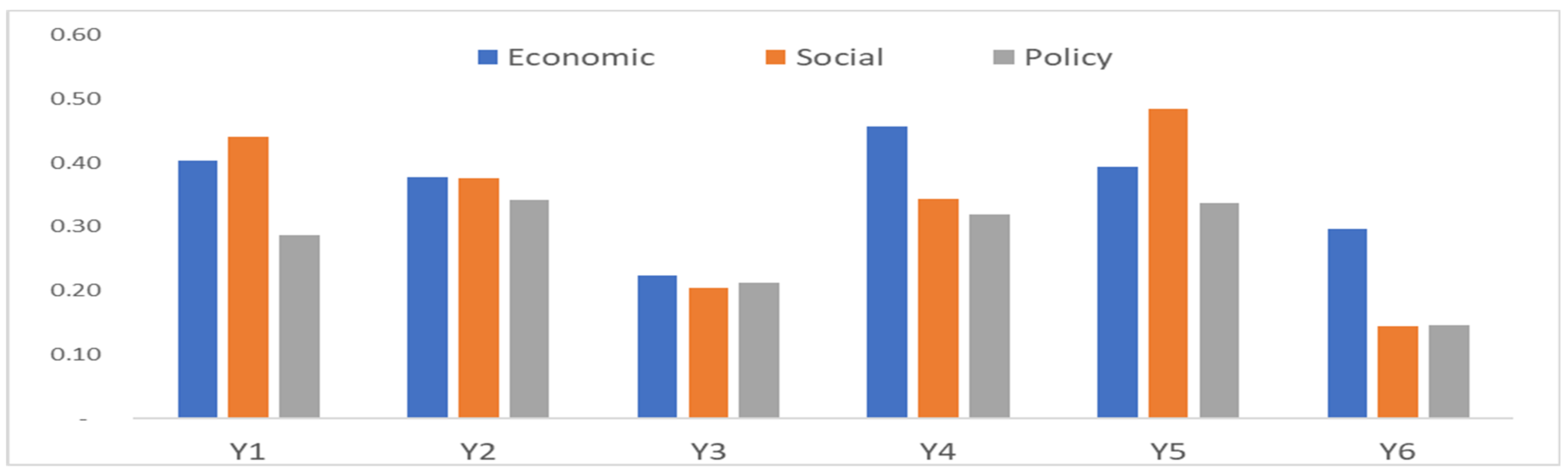
Table 1.
Interaction between Explanatory Variables.
| Graphical Representation | Description | Interaction |
|---|---|---|
 | q(∩) < Min(q(), q()) | Weaken, nonlinear |
 | Min(q(),q()) < q(∩) < Max(q()), q()) | Weaken, uni- |
 | q(∩) > Max(q(), q()) | Enhance, bi- |
 | q(∩) = q() + q() | Independent |
 | q(∩) > q() + q() | Enhance, nonlinear |


 .
.Table 2.
Model variable description.
| Variable | Index | Code | Type |
|---|---|---|---|
| Dependent Variable ) | Average Income of Urban Residents | Situation | |
| Average Income of Rural Residents | |||
| Urban–rural Income Gap Index | |||
| Changes in Average Income of Urban Residents | Dynamic | ||
| Changes in Average Income of Rural Residents | |||
| Changes in Urban–rural Income Gap Index | |||
| Independent Variable ) | Gross Domestic Product (GDP) | Economic driving force | |
| Per Capita GDP | |||
| Total Retail Sales of Consumer Goods | |||
| Added Value of Secondary Industry | |||
| Added Value of Tertiary Industry | |||
| Total Population | Social driving force | ||
| Floating Population | |||
| Urbanization Rate | |||
| Number of Internet users | |||
| Financial Expenditure | Policy driving force | ||
| Amount of Bank Loans | |||
| Main Functional Area Planning | |||
| Alleviating Poverty Policy |
Table 3.
Analysis of factor detector.
| q | 0.40 | 0.59 | 0.33 | 0.43 | 0.27 | 0.06 | 0.45 | 0.52 | 0.35 | 0.14 | 0.23 | 0.19 | 0.59 | |
| p | 0.00 | 0.00 | 0.00 | 0.00 | 0.02 | 0.20 | 0.00 | 0.00 | 0.00 | 0.03 | 0.00 | 0.01 | 0.00 | |
| q | 0.31 | 0.76 | 0.24 | 0.30 | 0.28 | 0.10 | 0.47 | 0.68 | 0.25 | 0.25 | 0.25 | 0.11 | 0.76 | |
| p | 0.01 | 0.00 | 0.01 | 0.01 | 0.01 | 0.05 | 0.00 | 0.00 | 0.01 | 0.03 | 0.03 | 0.03 | 0.00 | |
| q | 0.15 | 0.45 | 0.14 | 0.24 | 0.14 | 0.05 | 0.27 | 0.45 | 0.05 | 0.18 | 0.17 | 0.07 | 0.43 | |
| p | 0.02 | 0.00 | 0.04 | 0.05 | 0.03 | 0.05 | 0.01 | 0.00 | 0.05 | 0.04 | 0.05 | 0.05 | 0.00 | |
| q | 0.46 | 0.59 | 0.33 | 0.58 | 0.32 | 0.05 | 0.32 | 0.37 | 0.34 | 0.08 | 0.34 | 0.25 | 0.37 | |
| p | 0.00 | 0.00 | 0.00 | 0.00 | 0.00 | 0.17 | 0.00 | 0.00 | 0.00 | 0.06 | 0.00 | 0.00 | 0.01 | |
| q | 0.32 | 0.78 | 0.25 | 0.33 | 0.29 | 0.09 | 0.47 | 0.71 | 0.27 | 0.24 | 0.26 | 0.13 | 0.72 | |
| p | 0.00 | 0.00 | 0.03 | 0.00 | 0.01 | 0.08 | 0.00 | 0.00 | 0.01 | 0.04 | 0.02 | 0.02 | 0.00 | |
| q | 0.30 | 0.33 | 0.26 | 0.34 | 0.25 | 0.04 | 0.02 | 0.08 | 0.21 | 0.02 | 0.26 | 0.09 | 0.09 | |
| p | 0.00 | 0.00 | 0.01 | 0.00 | 0.04 | 0.22 | 0.27 | 0.04 | 0.05 | 0.16 | 0.00 | 0.03 | 0.03 |
Note: The average value of influence (q) of each factor is calculated at the significance level of 5% to represent the strength of economic, social and policy driving forces.
Publisher’s Note: MDPI stays neutral with regard to jurisdictional claims in published maps and institutional affiliations. |
© 2021 by the authors. Licensee MDPI, Basel, Switzerland. This article is an open access article distributed under the terms and conditions of the Creative Commons Attribution (CC BY) license (https://creativecommons.org/licenses/by/4.0/).
Share and Cite
MDPI and ACS Style
Zhang, P.; Li, W.; Zhao, K.; Zhao, S. Spatial Pattern and Driving Mechanism of Urban–Rural Income Gap in Gansu Province of China. Land 2021, 10, 1002. https://0-doi-org.brum.beds.ac.uk/10.3390/land10101002
AMA Style
Zhang P, Li W, Zhao K, Zhao S. Spatial Pattern and Driving Mechanism of Urban–Rural Income Gap in Gansu Province of China. Land. 2021; 10(10):1002. https://0-doi-org.brum.beds.ac.uk/10.3390/land10101002
Chicago/Turabian StyleZhang, Ping, Weiwei Li, Kaixu Zhao, and Sidong Zhao. 2021. "Spatial Pattern and Driving Mechanism of Urban–Rural Income Gap in Gansu Province of China" Land 10, no. 10: 1002. https://0-doi-org.brum.beds.ac.uk/10.3390/land10101002
Note that from the first issue of 2016, this journal uses article numbers instead of page numbers. See further details here.